A Novel Method for Obtaining the Loess Structural Index from Computed Tomography Images: A Case Study from the Lvliang Mountains of the Loess Plateau (China)

Abstract

The structural index is an important quantitative parameter for revealing the structural properties of loess. However, there is no a widely accepted measurement method for structural index at present. This study aims at presenting a novel method for obtaining the loess structural index (LSI), based on the application of computed tomography (CT) scanning techniques and laboratory physico-mechanical tests. The mountainous area of Lvliang in northwest China was taken as the study area, and Late Pleistocene loess samples were taken from various sites in the region. Several physical parameters were first measured using laboratory tests, including dry density, pore ratio, and liquidity index. CT scanning was used to observe sample microstructures, and a mathematical relationship was established between CT image parameters and the physical property indices, through three dimensions (3D) reconstruction and slice porosity analysis. The results revealed that LSI can be expressed as a non-linear function related to CT image parameters, dry density, and the liquidity index of the loess. Compared with traditional calculation methods, this novel technique calculates the LSI by using an empirical formula, which is less labor-intensive. Such results indicate that the method warrants wide application in the future.

1. Introduction

Loess forms through the deposition of aeolian sediments [1] in arid or semi-arid environments, so it normally has unique structural properties [2] and water sensitivity [3,4]. In many cases, such properties can result in negative effects, including extensive surface erosion [5,6] and catastrophic geological hazards [7,8,9]. Covering an estimated total area of 6.4 × 10⁵ km², the Loess Plateau has the most complex loess topography in China and, therefore, exhibits great environmental vulnerability to human activities [10,11]. Especially in recent years, frequent and intense disturbance by external factors, including human engineering activities [12,13] and extreme climate change [14,15], have exacerbated this vulnerability. Hence, loess is regarded as one of the problematic soils that requires attention in this region [16,17]. Moreover, knowing the situation and the solutions to one of the areas of the world affected by land degradation and desertification processes is relevant to achieve the sustainable development goals of the United Nations [18,19]. This will help to achieve the land degradation neutrality challenge [20].

Defined as a combination of soil fabric and interparticle bonding [21,22], the soil structure is essentially a kind of physical property. Hence, it is usually associated with the complex mechanical or physical behavior of soil fabric [23], such as pore size [24] and distribution [25] and aggregate arrangement [26,27]. However, such work cannot be used to directly obtain or characterize the structural strength of soil, which reflects the bonding energy between soil aggregates or units [1,23]. To remedy this, laboratory physical-mechanical tests should be performed to analyze the change in the connection between particles or structural units in soil, both before and after its structure is destroyed. However, the strength change of structured soil follows a non-linear law, making the Mohr–Coulomb criterion unsuitable for this type of soil.

Despite some constitutive models for structured soils having been proposed in the literature [28,29,30], they are seldom applicable to loess due to inherent limitations. Hence, some researchers used quantitative parameters to characterize the structural properties of loess. For instance, the traditional method measured soil structural potential parameter (also called soil structural index) by comparing the different strengths of undisturbed, remolded, and saturated soil [31,32,33]. However, various states of soil must be prepared for this test, making it a rather complex and laborious process. Fortunately, the initial structure of soil has a close correlation with basic physical indicators, that is, soil particle size, density, and humidity, respectively [34]. This provides a possible method to address the limitations of complexity. Hence, in the present work, this theory was selected as the basis for analyzing the mathematical relationship between the initial soil structural index and physical indicators.

In addition to the extensive discussions around physical-mechanical laboratory tests, in recent years, high-resolution imaging has been an important tool for studying the structural properties of soil, including digital cameras [35], scanning electron microscopy (SEM) [4], mercury intrusion porosimetry [36], electronic probes [37], magnetic resonance imaging [38], and the most widely used, computed tomography (CT) scanning. Recent experimental results have demonstrated that the CT technique could offer real-time information on the variation of some physical soil parameters occurring in the test specimen, such as the process of damage evolution [39], micro-mechanical properties [40], and porosity [41]. Hence, CT scanning can be used as a bridge between micro-scale and the macro-scale geomaterials [42]. Unfortunately, the application of this technique to determine the soil structural index remains a challenge. However, since the CT image reconstruction can be used to obtain a 3D model, effectively combining laboratory and numerical tests [43], a direct connection between the micro-structural parameters and structural index of soil is possible.

This study examines an area around the Lvliang Mountains (eastern Loess Plateau) in China. Since the loess deposition in the region is a typical structured soil, the main aim of the present study is to obtain the loess structural index (LSI) using instrumental methods. The specific objectives is to establish formula which can calculate the LSI from CT scanning images to reduce the labor-intensive works (e.g., unconfined compressive strength tests) used in traditional methods.

2. Materials and Methods

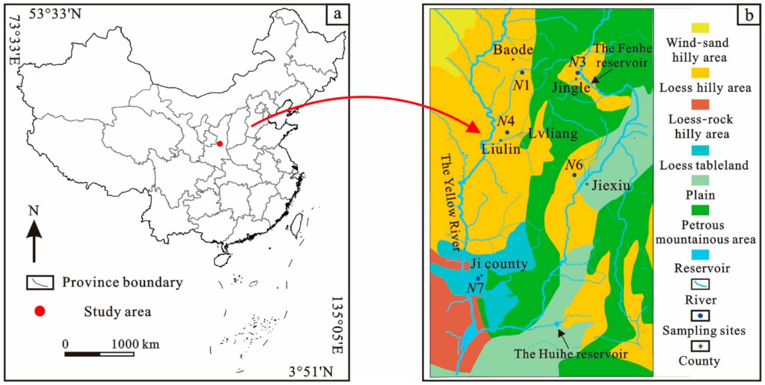
2.1. Study Area and Loess Samples

The Lvliang Mountains were chosen as the study area, which are located in the central and northern parts of China (Figure 1a). The region spans the Shanxi and Shaanxi provinces, of which the former contains most of the mountainous area. The total length of the region is more than 400 km with a width of 40~80 km. The mountains are mainly distributed in the western part of Shanxi Province, along a northeast-southwest direction. The elevation ranges from 1000 to 2800 m above sea level, characterized by high terrain in the north and low terrain in the south. The Yellow River is the main river system in the region and lies on the western side of the study area. The climate of the area is a continental monsoon climate. The average annual rainfall is about 400~800 mm, and the rainy season occurs in June~August. Due to the hilly and mountainous location, the climate shows obvious variation with vertical differences.

Loess samples were collected from five different counties in the region (Baode, Jingle, Liulin, Jiexiu, and Ji, respectively) (Figure 1b). The samples were collected using a hand-held spade and were extracted as a soil mass. The depths of the samples ranged from 3 to 16.5 m to ensure that all the samples were in the Late Pleistocene soil layer. Three typical geological layers consisting of loess soil were selected: L1 (Malan loess layer) [44], S1 (paleosol layer) [45], and L2 (Lishi loess layer) [46], respectively (Supplementary Materials S1). All these three are from the Chinese Soil Taxonomy (CST) [47]. In order to prevent moisture loss, all the samples were sealed with plastic film and tape after they were taken from the soil layer. A total of 15 undisturbed loess samples were obtained with dimensions of 30 cm × 30 cm × 30 cm.

2.2. Laboratory Test

To obtain the soil structural index, at least three types of soils are necessary, i.e., undisturbed, remolded, and saturated soils. The equation for the index is as follows [32]:

$$m_u=\frac{{\left(q_u\right)}_o{}^2}{{\left(q_u\right)}_r{\left(q_u\right)}_s}$$

(1)

where (q_u)_o, (q_u)_r, and (q_u)_s are the unconfined compressive strengths of undisturbed soil, saturated soil, and remolded soil, respectively. Meanwhile, m_u has a close connection with the comprehensive physical index (I_Lρ_d)/(ρ_we₀) [2] (with a correlation coefficient of up to 0.9 in some cases [34], where I_L denotes the liquidity index, ρ_d denotes dry density, ρ_w is pure water density, and e₀ is soil porosity. Hence, the relationship between the LSI and comprehensive physical index can be fitted if these values are obtained.

The physical properties experiments, including the moisture content testing, density testing, and limit moisture content testing, were performed on the undisturbed soil samples to obtain their physical indicators. It should be noted that all the test methods followed the relevant industry standards of China and were performed according to the given steps (Supplementary Materials S2).

The samples selected for the unconfined compressive strength test were prepared with the same size of Φ 39.1 mm × H 80 mm and the same dry density. In addition, the moisture content of the remolded samples should be the same as that of the undisturbed samples. The preparation of remolded samples can be seen in the supplementary material (Supplementary Materials S2). A unconfined pressure tester was used to measure the compressive strengths of the samples with a shear rate of 3 mm/min. When the number of manual turns reaches 18, the equipment will rise by 1 mm. The values of the axial dynamometer were recorded whenever the axial displacement reached 0.1 mm. In order to obtain a more continuous stress–strain curve, the test data were photographed and manual recorded at the same time. The equipment tested three samples with the same state at the same time, and the average values of the unconfined compressive strengths of the three samples were considered as the final result.

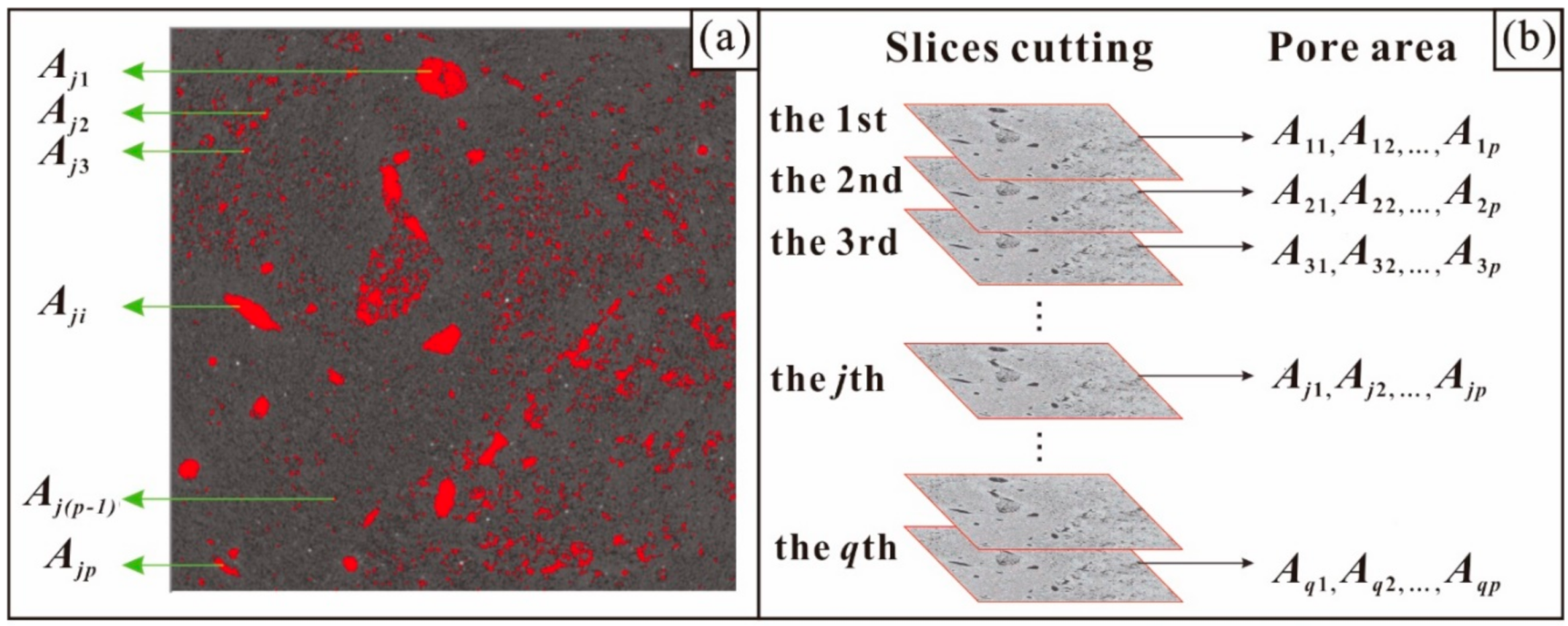
2.3. Computerized Tomography (CT) Scanning

Computerized tomography scanning, which was first applied in the medical field, has been widely used in recent years to solve geotechnical problems [48]. As a non-destructive characterization method, this technique is helpful for visualizing and quantitatively measuring the internal structure of samples [42]. In this study, CT scanning of undisturbed soil was performed on XTH225ST machine produced by NIKON company (https://www.nikon.com/, accessed on 20 October 2020), in the Industrial CT Scanning Laboratory of China University of Geosciences (Beijing, China). It should be noted that only four samples (samples 1-1, 6-1, 6-2, and 6-3) were selected for CT scanning owing to the limitation of the workload and the complexity of the subsequent analysis process. Because a smaller sample size can ensure a higher image resolution, the samples were prepared as cylinders with a size of Φ 20 mm × H 20 mm. The 225 kV barrel was selected as the X-ray generator, and the parameters in the scanning process were set as follows: (i) 135 kV tube voltage; (ii) 57 μA tube current; (iii) the scanning time of a single photo was 1 s; (iv) the scanning method was translation-rotation (TR) mode; (v) the image resolution was 14 μm. The CT images were obtained in TIFF format and then preprocessed with Gaussian noise-reduction filters and brightness and contrast adjustments (to improve the quality of the final model). CT Pro 3D was then used to reconstruct the images into a 3D model of each soil sample. Finally, the reconstructed 3D model was cut into many slices, each one pixel thick, using the VG Studio Max software. The output images, in Image Stack format, were then analyzed visually.

The 3D model and slices images obtained from CT scanning can clearly be used to characterize the microstructure of a sample, especially the pore size and its distribution [24,25]. Hence, the mathematical relationship between the CT image parameters and the pore index can be established through the analysis of pore volume. According to the traditional theory of soil mechanics, the density and volume of the soil can be calculated using Equations (2) and (3), respectively, as follows:

$$\rho =\frac{m}{V}=\frac{m_s(1+W_0)}{V}$$

(2)

$$V=(1+\frac{1}{e_0})V_v$$

(3)

where ρ, m, and V are the natural density, weight, and total volume of the soil, respectively, m_s is the weight of the soil particles, W₀ is the natural moisture content, V_v is the volume of the pores, and e₀ is the pore ratio. Hence, the natural density of soil can also be expressed as follows:

$$\rho =\frac{m_s(1+W_0)}{V}=\frac{(1+W_0)e_0}{(1+e_0)}\times \frac{m_s}{V_v}$$

(4)

The index V_v can also be determined from microstructure images. For the 3D model of a specific soil sample, if the model was cut into q slices and the number of pores in each slice was p, the total volume of pores in the model can be calculated as follows:

$$V_v={\displaystyle \sum _{j=1}^q{\displaystyle \sum _{i=1}^p(A_{ji}\cdot R_j)}}$$

(5)

where A_ji is the area of the i-th pore in the j-th slice (Figure 2a), and R_j is the thickness of the slice, which is a fixed value in our work (i.e., one pixel). The total volume of the soil (Figure 2b) can be calculated as:

$$V=\frac{V_v}{n}$$

(6)

where n denotes the porosity of the soil. By setting n_j as the areal porosity of the j-th slice, the following expression can be obtained:

$$V=\frac{V_v}{n}={\displaystyle \sum _{j=1}^q(\frac{{\displaystyle \sum _{i=1}^p{A}_{ji}}}{n_j}}\cdot R_j)$$

(7)

In addition, the weight of soil particles m_s, the total volume V, dry soil density ρ_d and soil porosity n have the following relationship:

$$m_s={\rho }_d\times V=\frac{{\rho }_d\times V_v}{n}$$

(8)

By substituting Equation (7) into Equation (8), the expression can be derived as follows:

$$m_s={\rho }_d\times {\displaystyle \sum _{j=1}^q(\frac{{\displaystyle \sum _{i=1}^p{A}_{ji}}}{n_j}}\cdot R_j)$$

(9)

If Equations (5) and (9) are substituted into Equation (4), the relationship between physical indicator (i.e., the pore ratio e₀) and microstructure image parameters can be obtained as follows:

$$1+\frac{1}{e_0}={\displaystyle \sum _{j=1}^q(\frac{{\displaystyle \sum _{i=1}^p{A}_{ji}}}{n_j}\cdot R_j)}/{\displaystyle \sum _{j=1}^q{\displaystyle \sum _{i=1}^p(A_{ji}\cdot R_j)}}$$

(10)

3. Results

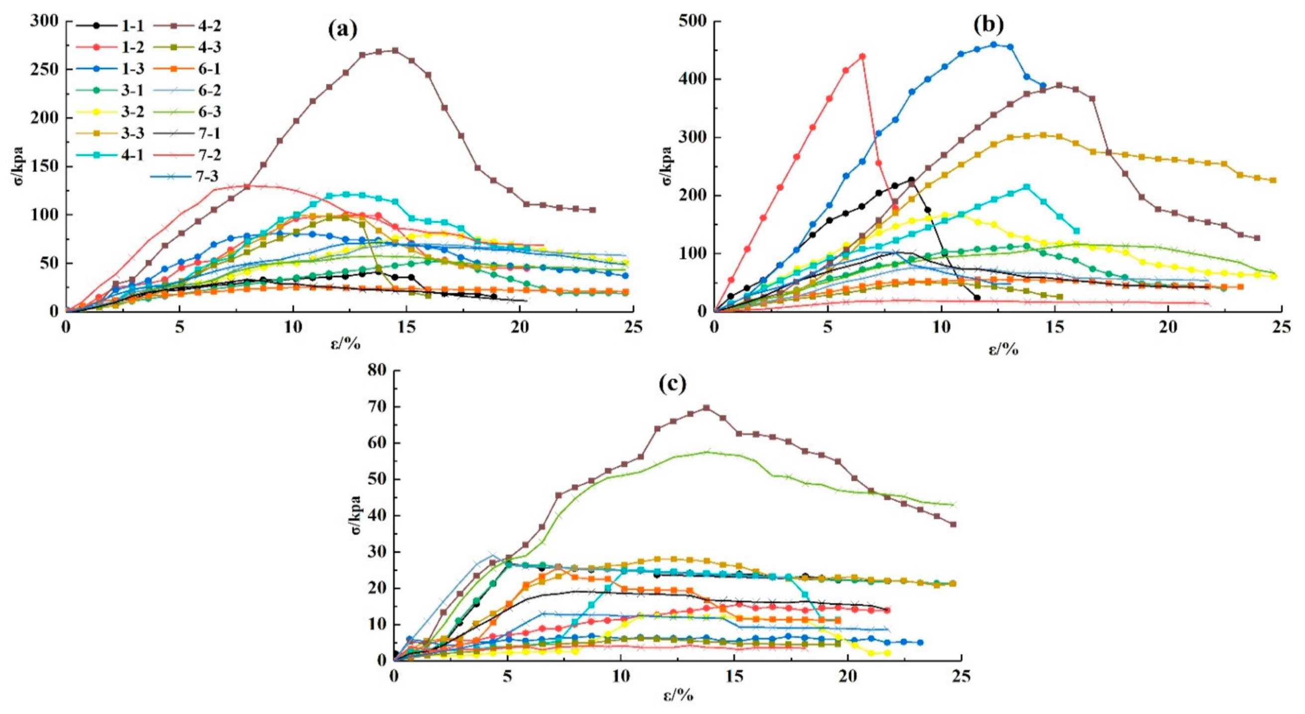
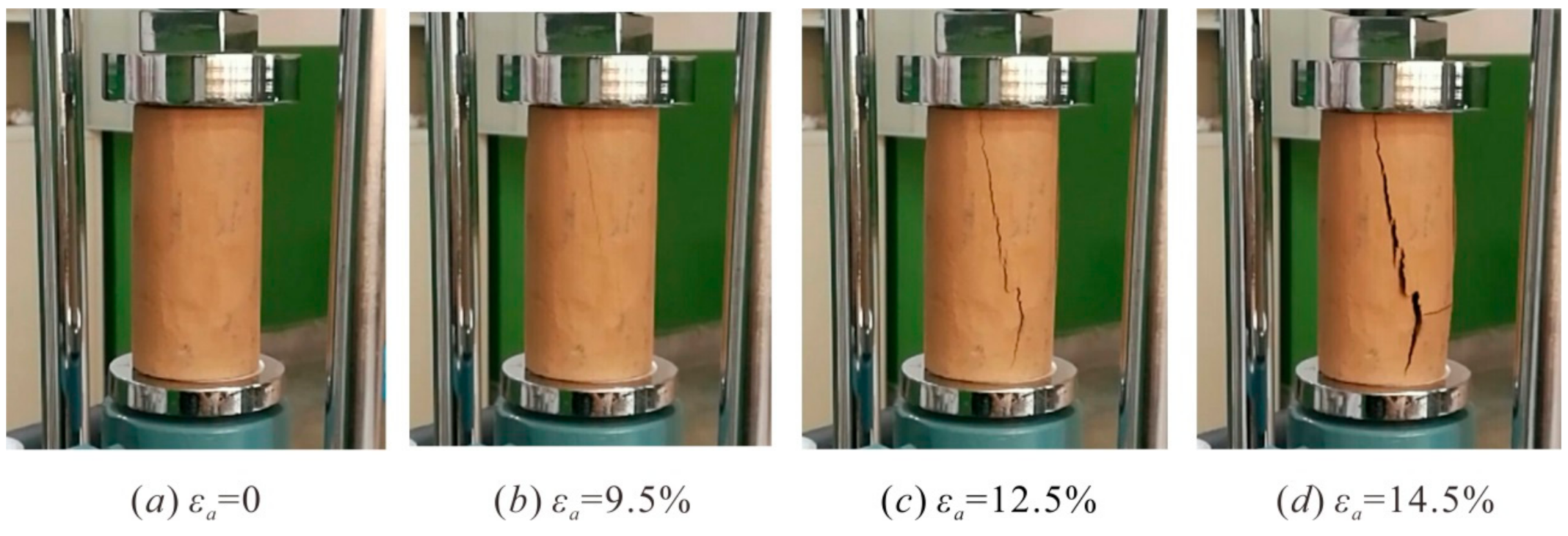
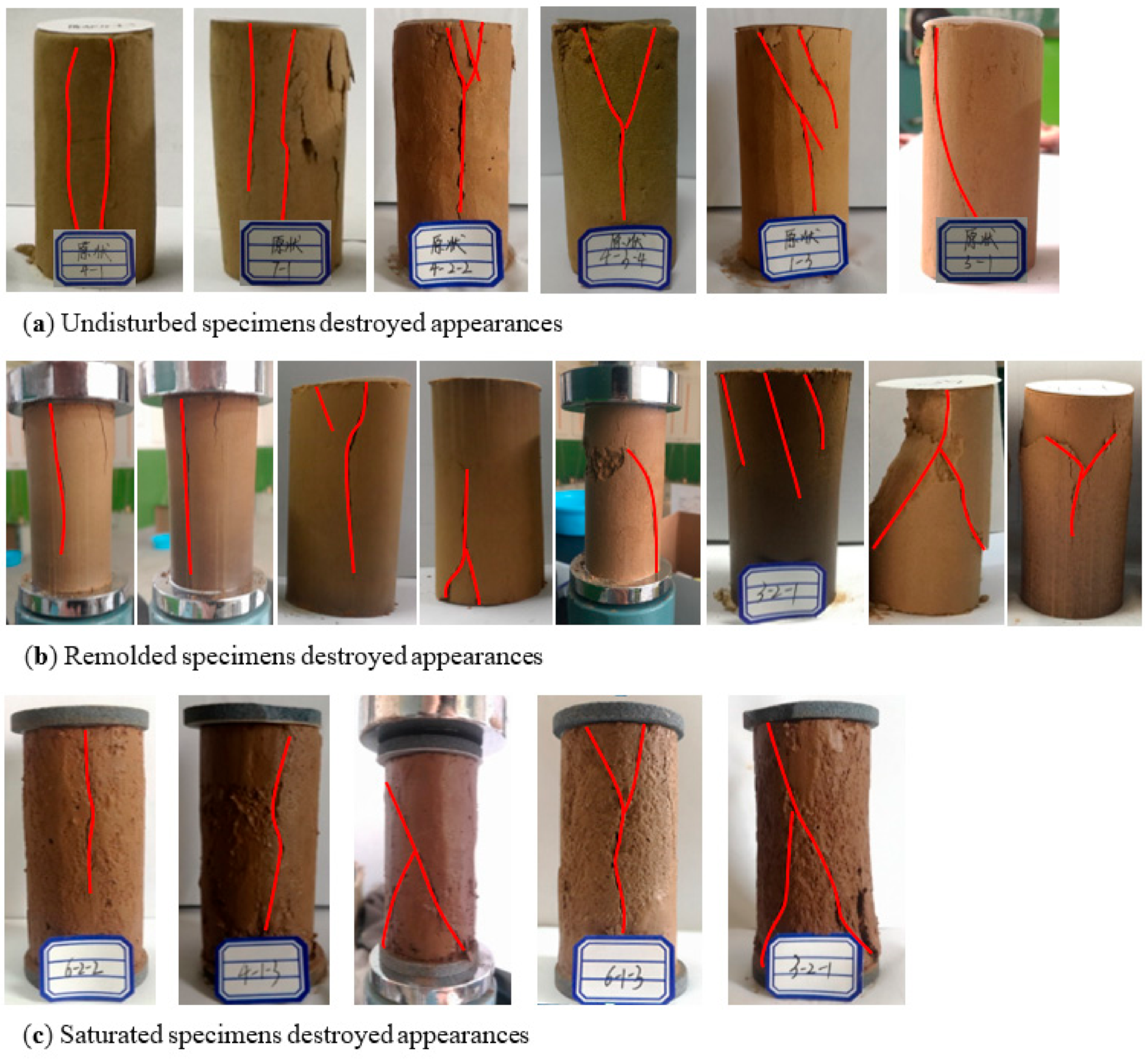
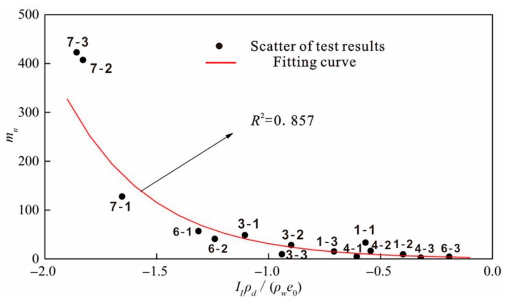
3.1. Results of Laboratory Tests

As seen in Figure 3, the samples exhibited typical class I stress-strain curve, that is, with a negative slope in the post-peak phase. During the elastic deformation phase, the internal structures of the samples were continuously adjusted under an external load, along with the initial destruction. With a further increase in the axial stress, micro-cracks began to appear and extended continuously. When the peak strength was reached, the soil was destroyed, and the slope of the curve inversed immediately. The width of the cracks then increased sharply, and the curve gradually decreased to a point representing the residual strength. A typical destruction process of the undisturbed samples can be seen in Figure 4 (taking the sample 1-1 as the example), which consists of four main phases: (i) the initial state of the sample, (ii) the phase of elastic deformation, (iii) the failure of the sample, and (iv) the phase of residual deformation. In terms of the resulting unconfined compressive strength values for the different layers, L1 ranged from 55.56 to 226.39 kPa, whereas S1 and L2 had strengths of 75.46~437.82 kPa and 51.11~458.96 kPa. The largest unconfined compressive strength of all three layers was located in Baode County (i.e., the N1 sampling site). Most of the samples were completely destroyed when the strain was less than 15%. In addition, for samples in the same layer, the rank of the unconfined compressive strength was: undisturbed samples > remolded samples > saturated samples, indicating that the structural property of the loess plays an important role in soil strength.

Under the effect of external loading, soil particles will slide and rotate, with microcracks developing and spreading continuously and appearing as cracks and macroscopic sample failure. As seen in Figure 5, according to the shape and direction of the cracks, the failure modes of the samples can be divided into five types: (i) linear splitting, (ii) Y-type splitting, (iii) diagonal shear, (iv) wedge shear, and (v) Y-type shear failure. Category (i), (ii), and (iii) can be seen in the undisturbed samples (Figure 5a). The remolded samples (Figure 5b) exhibited all failure modes except the (ii), whereas the saturated samples exhibited only linear splitting failure and Y-type shear failure (Figure 5c). The statistical results indicated that Y-type shear failure was the main failure mode in the undisturbed and saturated samples, while the remolded samples were dominated by wedge shear failure. The cracks on the failure surfaces of the remolded samples occurred in relatively arrangements and shapes, and the direction of the cracks were similar, with a small number of inflection points. In contrast, the cracks in the undisturbed samples had more extension directions and more inflection points. This is possibly because the preparation process of the remolded samples made their soil structures more homogeneous than that of the undisturbed samples. The undisturbed samples, influenced by the forming mechanism of loess, may have quite large heterogeneity of soil structures, causing the cracks to extend along the weak places first under loading conditions. Compared with the undisturbed samples, all the pores of the saturated samples were filled with water, which enhanced the heterogeneity of the soil structures, so more irregular cracks formed in the saturated samples.

The stress–strain curves were analyzed to obtain the unconfined compressive strength of soil samples in different states, and are shown in

Table 1. Physical indicators obtained from laboratory tests and the calculated soil structure index of the collected loess samples.

Sample ID	Dry Density ρd (g/cm3)	Pore Ratio e0	Liquidity Index IL	Physical Index ILρd/(ρwe0)	Unconfined Compressive Strength (kPa)			Structural Index mu
					Undisturbed q0	Remolded qr	Saturated qs
1-1	1.35	0.99	−0.81	−1.10	226.39	40.39	26.15	48.52
1-2	1.52	0.78	−0.85	−1.66	437.82	99.04	15.18	127.48
1-3	1.49	0.84	−1.05	−1.86	458.96	78.61	6.34	422.76
3-1	1.33	1.03	−0.73	−0.94	112.84	51.65	26.15	9.43
3-2	1.52	0.78	−0.46	−0.90	166.98	80.35	12.28	28.26
3-3	1.35	0.98	−0.41	−0.56	303.88	99.02	28.01	33.30
4-1	1.33	1.03	−0.55	−0.71	213.81	120.78	24.76	15.29
4-2	1.55	0.75	−0.60	−1.24	388.89	268.30	13.78	40.91
4-3	1.44	0.97	−0.13	−0.19	51.11	96.62	6.09	4.44
6-1	1.35	1.00	−0.45	−0.61	55.56	24.76	25.55	4.88
6-2	1.45	0.86	−0.19	−0.32	75.46	70.07	28.99	2.80
6-3	1.45	0.87	−0.24	−0.40	115.79	57.02	25.35	9.27
7-1	1.25	1.15	−0.50	−0.54	101.42	32.96	19.02	16.41
7-2	1.45	0.87	−1.10	−1.83	365.34	129.31	2.54	407.10
7-3	1.39	0.94	−0.89	−1.32	102.22	71.27	2.58	56.92

with the physical indicators of the samples.

Subsequently, these values were used to calculate the soil structure index according to Equation (1). The fitting curve between the LSI and the comprehensive physical index (I_Lρ_d)/(ρ_we₀) is shown in Figure 6, and their mathematical connection can be expressed as follows:

$$m_u\approx 2.2979\times e^{-2.61\frac{I_L{\rho }_d}{{\rho }_w{e}_0}}\hspace{1em}(R^2=0.857)$$

(11)

where ρ_w is the density of water, which is generally considered to be 1.0 g/cm³. Hence, Equation (11) can be simplified as follows:

$$e_0\approx 2.61\frac{I_L{\rho }_d}{\ln 2.2979-\ln m_u}$$

(12)

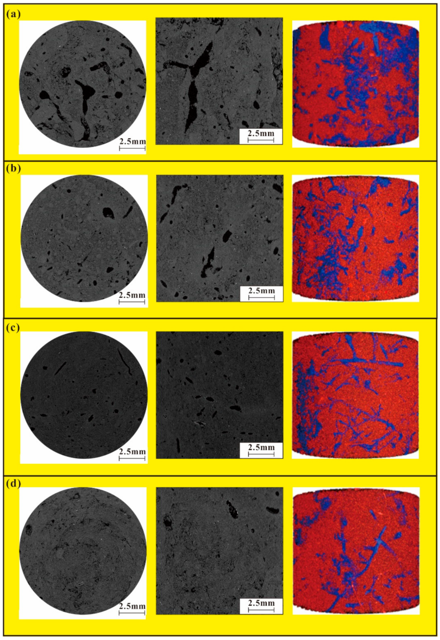
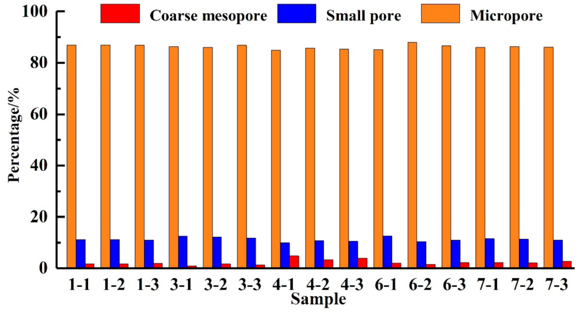
3.2. Results of CT Scanning

The reconstructed 3D models of the samples were shown in Figure 7. The blue areas indicate pores while red indicates soil particles. It is clear that the pore distribution was rather uneven, which represents that the samples had high heterogeneity. VG Studio Max software was used to analyze the pore properties of the samples, including the number of pores, pore volume, and porosity of the samples. In this process, the minimum probability that the software recognized the pores was set to 5%. The whole sample was selected as the region of interest (ROI). The final results can be seen in

Table 2. The pore characteristics of all the samples.

Sample	Sampling Depth/m	Total Volume/μm3	Porosity/%	Volume of the Soil Particles/μm3	Volume of the Pores/μm3	Amount of the Pores
1-1	3	4214.33	16.28	3528.24	686.09	102,685
1-2	5	4214.33	13.40	3649.61	564.72	103,452
1-3	10	4214.33	11.58	3726.31	488.02	110,246
3-1	3	4214.33	11.66	3722.94	491.39	108,795
3-2	7	4214.33	12.34	3694.28	520.05	104,335
3-3	9	4214.33	10.61	3767.19	447.14	105,324
4-1	3	4214.33	9.89	3797.53	416.80	156,039
4-2	14	4214.33	8.96	3836.73	377.60	135,986
4-3	16.5	4214.33	7.12	3914.27	300.06	184,345
6-1	3	4214.33	10.24	3782.78	431.55	144,770
6-2	3.5	4214.33	6.23	3951.78	262.55	177,705
6-3	4.5	4214.33	8.93	3837.99	376.34	119,389
7-1	3	4214.33	11.92	3711.98	502.35	129,583
7-2	7.5	4214.33	13.25	3655.93	558.40	149,248
7-3	13.5	4214.33	10.06	3790.37	423.96	159,328

. It should be noted that due to the size uncertainty of the ROI selected by the software, the pore characteristics in the table represent the normalized data. Overall, with an increase in the sampling depth, the 3D porosity of the samples decreased. In addition, the porosity of the L2 layer was less than that of the S1 and L1 layers. The pores were divided into four categories based on diameter (D): (i) micropores (D ≤ 100 μm), (ii) small pores (100 μm ≤ D ≤ 200 μm), (iii) coarse mesopores (200 μm ≤ D ≤ 1000 μm), and (iv) macropores (D ≥ 1000 μm). As seen in Figure 8, the percentage of micropores in the loess of Baode County (sample 1-1, 1-2 and 1-3) was slightly higher than that in other samples. The percentage of coarse mesopores in samples 3-1, 3-2, and 3-3 was much lower than in the other samples. This is considered to be associated with the content of clay particles. The pores formed between these particles were generally smaller than between other types of particles and could be filled by fine substances.

Since the pore ratio e₀ exists in both Equations (10) and (12), the relationship between the LSI and CT image parameters can be obtained by combining the two equation as follows:

$$1+\frac{\ln 2.2979-\ln m_u}{2.61I_L{\rho }_d}\approx {\displaystyle \sum _{j=1}^q(\frac{{\displaystyle \sum _{i=1}^p{A}_{ji}}}{n_j}\cdot R_j)}/{\displaystyle \sum _{j=1}^q{\displaystyle \sum _{i=1}^p(A_{ji}\cdot R_j)}}$$

(13)

Based on this, the quantitative calculation formula of LSI can be determined as follows:

$$\ln m_u\approx \ln 2.2979-2.61I_L{\rho }_d\left[{\displaystyle \sum _{j=1}^q(\frac{{\displaystyle \sum _{i=1}^p{A}_{ji}}}{n_j}\cdot R_j)}/{\displaystyle \sum _{j=1}^q{\displaystyle \sum _{i=1}^p(A_{ji}\cdot R_j)}}-1\right]$$

(14)

From this equation, we can see that the loess structural index can be expressed by a non-linear function related to CT image parameters, dry density, and liquidity index of the soil. In particular, all the variables used in this formula are related only to undisturbed soil. Hence, it is not necessary to prepare the remolded and saturated samples and measure their unconfined compressive strengths. This proposed method is, therefore, more convenient and less laborious than traditional methods.

4. Discussion

The recognition of the pores in each slice depends on the ROI settings. As a type of supervised classification method, the selection of the ROI has a noticeable impact on the effects of classification. Generally, for samples with obvious spatial heterogeneity (like in this study), it is not possible to map the true variation of the pore indices (e.g., areal porosity, total area of the pores in each slice, etc.) without very dense sampling over the overall sample [49]. Even in a strict sense, the error or uncertainty introduced by the heterogeneity of the pores still remains a big challenge in the CT scanning tests, because true homogeneity is almost impossible in nature [50]. However, a large number of sampling operations enhance both the labor cost and the occurrence probability of errors. Fortunately, the application of visual analysis software provides a solution to address this problem. In our study, VG Studio software was used to obtain the pore parameters. The large soil samples were first cut into many slices, after which the pore and soil particles were counted. Because all the pores that were identified, according to the conditions by set the user, were included in the final result, an assessment of pore spatial heterogeneity is not necessary.

For the convenience of the scanning operations and subsequent slice analysis, most studies prepared the soil samples for CT scanning as cylinder shapes [25]. However, it should be noted that all the soil samples in this study were made manually; thus, strictly speaking, they only approximated a cylinder, due to artificial errors. The XTH225ST CT scanning machine determined the resolution of the final images as it adjusts to the size of each sample. Therefore, not all samples returned images with resolutions of 14 μm (this value can be seen in Section 2.1.). Rather, the image resolutions of the four soil samples in this study were 13.71 μm, 13.71 μm, 13.51 μm and 13.51 μm, which subsequently led to different slice thickness in VG Studio Max. Similarly, each sample was divided into a different number of slices. Another impact of the varying image resolutions on the resulting of loess structural index was reflected in the pore statistics. Even though the image resolutions were rather high, pores less than 14 μm in size still not included in the statistics. Rather, such pores were categorized as soil particles, resulting in a smaller areal porosity. The SEM results also support this assumption: the areal porosity obtained through SEM (Figure 9) were larger than those obtained through CT scanning. An important reason for this difference is that SEM can reach nanometer-scale resolutions, which is higher than that of the CT test. Certainly, the application of the software for digital processing of CT scanning images cannot be ignored. All of the images obtained from CT tests were greyscale images, so pore and soil particle recognition was performed using VG Studio software. Although we have tried to reduce the artificial errors by selecting clearer ROIs and setting parameters (e.g., grey value) to more appropriate values, some pores were still incorrectly classified as soil particles. Hence, due to pores being smaller than the image resolution, limitations of image-processing software, and estimated formulas, the obtained results may have considerable uncertainties, especially for the samples that were not very regular in the shape, and in the ROIs containing many small pores. At the same time, we cannot effectively determine the influence of these errors on the final calculation (whether they overestimate or underestimate the results) because the LSI calculation formula associated with these parameters is a non-linear function. In this context, the standardization of the test process, including sample preparation, ROI selection, and software parameter settings, becomes very important for obtaining more accurate results.

Although the method presented here can be used to obtain the soil structural index associated with the microstructure images parameters, the coefficients appearing in the estimated formula were not be proven to be universally applicable. Therefore, the purpose of this study is not to propose a widely applicable model, but to discuss the connection between the LSI and CT scanning images. Hence, a similar analysis could be adopted to determine the corresponding calculation formula applicable to other regions. Certainly, a unified formula at the regional scale is also possible if enough soil samples are prepared and a large number of experiments are carried out, which definitely calls for considerable work and cost. However, it should be noted that a widely applicable formula may only apply in a statistical sense, and more detailed experimental designs will still be necessary to obtain more accurate results. From the perspective of parameters in the formula (Equation (14)), it still requires two physical parameters (the liquidity index and dry density of the loess sample), in addition to the CT image parameters. These physical parameters are mainly related to the physical implications of the soil structure index. The traditional method [32] of calculating the LSI can explain this point: a saturated sample is required in the experiment, illustrating the influence of soil moisture content on LSI. However, as physical parameters, the liquidity index and dry density of soil also have certain morphological implications. If adequate and accurate efforts are made, it may be possible to establish a quantitative relationship between morphological parameters and soil structural index, so that physical parameters are no longer required.

Last but not least, although this study only deals with the loess structure, it would be helpful for finding the proper land management measures in fragile environments such as the loess belt in China. Many studies have identified the soil erosion and soil loss with soil structure, whereas elevated soil loss and runoff rates can reduce soil fertility [51], which subsequently cause a series of problems. Hence, to achieve the United Nations sustainable development goals, it is necessary to explore new measurement techniques of structured soils. Given that many attempts have been conducted in land management, such as the cover crop management [52] and long-term soil erosion monitoring and measurement [53], the proposed procedure in this study would be a useful supplement to improve the soil conditions and avoid soil erosion and land degradation.

5. Conclusions

This study proposed a novel method for obtaining the loess structural index by using the CT scanning. Based on several laboratory tests and slice porosity analysis of the reconstructed 3D model of loess samples, both the soil structural index and parameters of CT scanning images were linked with the physical indicators of the samples. Hence, a mathematical formula showing the empirical relationship between CT scanning image parameters and the soil structural index in the area could be established. The Late Pleistocene loess in the Lvliang Mountains (China) was used as a case study to clarify the application procedure. The expression of the soil structural index obtained via this method is a non-linear function associated with the CT image parameters, liquidity index and dry density of the loess samples. These results indicate that the soil structural index can be measured and calculated using two simple tests for soil density and limit moisture content, as well as CT scanning. Compared with traditional methods, the time-consuming strength tests on remolded soil and saturated soil can be avoided in the proposed method, so the workload is smaller. Moreover, the method is beneficial for the prevention of geo-hazards associated with loess, and contribute to meeting the land degradation neutrality challenge.

References

1. Ng, C.W.W.; Sadeghi, H.; Hossen, S.K.B.; Chiu, C.F.; Alonso, E.E.; Baghbanrezvan, S. Water retention and volumetric characteristics of intact and re-compacted loess. Can. Geotech. J. 2016, 53, 1258–1269. [Google Scholar] [CrossRef]
2. Shao, S.; Wang, L.; Tao, H.; Wang, Q.; Wang, S. Structural index of loess and its relation with granularity, density and humidity; in Chinese with English abstract. Chin. J. Geotech. Eng. 2014, 36, 1387–1393. [Google Scholar]
3. Assallay, A.M.; Rogers, C.D.F.; Smalley, I.J. Formation and collapse of metastable particle packings and open structures in loess deposits. Eng. Geol. 1997, 48, 101–115. [Google Scholar] [CrossRef]
4. Zhang, F.; Wang, G.; Kamai, T.; Chen, W.; Zhang, D.; Yang, J. Undrained shear behavior of loess saturated with different concentrations of sodium chloride solution. Eng. Geol. 2013, 155, 69–79. [Google Scholar] [CrossRef] [Green Version]
5. Wei, W.; Chen, L.; Fu, B.; Huang, Z.; Wu, D.; Gui, L. The effect of land uses and rainfall regimes on runoff and soil erosion in the semi-arid loess hilly area, China. J. Hydrol. 2007, 335, 247–258. [Google Scholar] [CrossRef]
6. Wei, W.; Chen, L.; Zhang, H.; Yang, L.; Yu, Y.; Chen, J. Effects of crop rotation and rainfall on water erosion on a gentle slope in the hilly loess area, China. Catena 2014, 123, 205–214. [Google Scholar] [CrossRef]
7. Derbyshire, E. Geological hazards in loess terrain, with particular reference to the loess regions of China. Earth Sci. Rev. 2001, 54, 231–290. [Google Scholar] [CrossRef]
8. Peng, J.; Leng, Y.; Zhu, X.; Wu, D.; Tong, X. Development of a loess-mudstone landslide in a fault fracture zone. Environ. Earth Sci. 2016, 75, 658–668. [Google Scholar] [CrossRef]
9. Tang, Y.; Feng, F.; Guo, Z.; Feng, W.; Li, Z.; Wang, J.; Sun, Q.; Ma, H.; Li, Y. Integrating principal component analysis with statistically-based models for analysis of causal factors and landslide susceptibility mapping: A comparative study from the loess plateau area in Shanxi (China). J. Clean. Prod. 2020, 277, 124159. [Google Scholar] [CrossRef]
10. Zhou, J.; Zhu, C.; Zheng, J.; Wang, X.; Liu, Z. Landslide disaster in the loess area of China. J. For. Res. 2002, 13, 157–161. [Google Scholar]
11. Wang, R.; Dong, Z.; Zhou, Z.; Wang, P. Temporal variation in preferential water flow during natural vegetation restoration on abandoned farmland in the Loess Plateau of China. Land 2019, 8, 186. [Google Scholar] [CrossRef] [Green Version]
12. Wang, J.; Liang, Y.; Zhang, H.; Wu, Y.; Lin, X. A loess landslide induced by excavation and rainfall. Landslides 2014, 11, 141–152. [Google Scholar] [CrossRef]
13. Zhuang, J.; Peng, J. A coupled slope cutting—A prolonged rainfall-induced loess landslide: A 17 October 2011 case study. Bull. Eng. Geol. Environ. 2014, 73, 997–1011. [Google Scholar] [CrossRef]
14. Tang, Y.; Xue, Q.; Li, Z.; Feng, W. Three modes of rainfall infiltration inducing loess landslide. Nat. Hazards. 2015, 79, 137–150. [Google Scholar] [CrossRef]
15. Zhang, M.; Liu, J. Controlling factors of loess landslides in western China. Environ. Earth Sci. 2010, 59, 1671–1680. [Google Scholar] [CrossRef]
16. Ma, F.; Yang, J.; Bai, X. Water sensitivity and microstructure of completed loess. Transp. Geotech. 2017, 11, 41–56. [Google Scholar] [CrossRef]
17. Wang, Y.; Li, Y.; Li, Y. Land engineering consolidates degraded sandy land for agricultural development in the largest sandy land of China. Land 2020, 9, 199. [Google Scholar] [CrossRef]
18. Keesstra, S.D.; Bouma, J.; Wallinga, J.; Tittonell, P.; Smith, P.; Cerdà, A.; Montanarella, L.; Quinton, J.N.; Pachepsky, Y.; van der Putten, W.H.; et al. The significance of soils and soil science towards realization of the United Nations Sustainable Development Goals. Soil 2016, 2, 111–128. [Google Scholar] [CrossRef] [Green Version]
19. Visser, S.; Keesstra, S.; Maas, G.; De Cleen, M. Soil as a Basis to Create Enabling Conditions for Transitions Towards Sustainable Land Management as a Key to Achieve the SDGs by 2030. Sustainability 2019, 11, 6792. [Google Scholar] [CrossRef] [Green Version]
20. Keesstra, S.; Mol, G.; De Leeuw, J.; Okx, J.; De Cleen, M.; Visser, S. Soil-related sustainable development goals: Four concepts to make land degradation neutrality and restoration work. Land 2018, 7, 133. [Google Scholar] [CrossRef] [Green Version]
21. Koliji, A.; Vulliet, L.; Laloui, L. Structural characterization of unsaturated aggregated soil. Can. Geotech. J. 2010, 47, 297–311. [Google Scholar] [CrossRef]
22. Mitchell, J.K. Fundamentals of Soil Behavior; John Wiley & Sons: New York, NY, USA, 1993. [Google Scholar]
23. Chen, H.; Jiang, Y.; Gao, Y.; Yuan, X. Structural characteristics and its influencing factors of typical loess. Bull. Eng. Geol. Environ. 2018, 78, 4893–4905. [Google Scholar] [CrossRef]
24. Zhang, W.; Sun, Y.; Chen, W.; Song, Y.; Zhang, J. Collapsibility, composition, and microfabric of the coastal zone loess around the Bohai Sea, China. Eng. Geol. 2019, 257, 105142. [Google Scholar] [CrossRef]
25. Li, P.; Xie, W.; Pak, R.Y.S.; Vanapalli, S.K. Microstructural evolution of loess soils from the Loess Plateau of China. Catena 2019, 173, 276–288. [Google Scholar] [CrossRef]
26. Mokritskaya, T.P.; Tushev, A.V.; Samoylich, K.A.; Baranov, P.N. Deformations of loess soils caused by changes in the microaggregate structure. Bull. Eng. Geol. Environ. 2019, 78, 3729–3739. [Google Scholar] [CrossRef]
27. Li, Y.; Zhang, T.; Zhang, Y.; Xu, Q. Geometrical appearance and spatial arrangement of structural blocks of the Malan loess in NW China: Implications for the formation of loess columns. J. Asian Earth Sci. 2018, 158, 18–28. [Google Scholar] [CrossRef]
28. Baudet, B.; Stallebrass, S. A constitutive model for structured clays. Geotechnique 2004, 54, 269–278. [Google Scholar] [CrossRef]
29. Suebsuk, J.; Horpibulsuk, S.; Liu, M. A critical state model for overconsolidated structured clays. Comput. Geotech. 2011, 38, 648–658. [Google Scholar] [CrossRef]
30. Robin, V.; Javadi, A.A.; Cuisinier, O.; Masrouri, F. An effective constitutive model for lime treated soils. Comput. Geotech. 2015, 66, 189–202. [Google Scholar] [CrossRef]
31. Shao, S.; Zhou, F.; Long, J. Structural properties of loess and its quantitative parameter; in Chinese with English abstract. Chin. J. Geotech. Eng. 2004, 26, 531–536. [Google Scholar]
32. Shao, S.; Zheng, W.; Wang, Z.; Wang, S. Structural index of loess and its testing method; in Chinese with English abstract. Rock Soil Mech. 2010, 31, 15–19. [Google Scholar]
33. Wang, L.; Shao, S.; Lu, Z. Influence of physical properties on the initial structure of loess. Rock Soil Mech. 2017, 38, 3484–3490. [Google Scholar]
34. Qin, P.; Shao, S.; An, Z.; Zhu, F.; Zheng, X. The initial state of the soil structural quantitative research and verification; in Chinese with English abstract. J. Xi’an Univ. Technol. 2015, 31, 448–453. [Google Scholar]
35. Yue, Z.; Chen, S.; Tham, L.G. Finite element modeling of geomaterials using digital image processing. Comput. Geotech. 2003, 30, 375–397. [Google Scholar] [CrossRef]
36. Sasanian, S.; Newson, T.A. Use of mercury intrusion porosimetry for microstructural investigation of reconstituted clays at high water contents. Eng. Geol. 2013, 158, 15–22. [Google Scholar] [CrossRef]
37. Gomez-Gonzalez, M.A.; Garcia-Guinea, J.; Laborda, F.; Garrido, F. Thallium occurrence and partitioning in soils and sediments affected by mining activities in Madrid province (Spain). Sci. Total Environ. 2015, 536, 268–278. [Google Scholar] [CrossRef] [Green Version]
38. Herrmann, K.H.; Pohlmeier, A.; Gembris, D.; Vereecken, H. Three-dimensional imaging of pore water diffusion and motion in porous media by nuclear magnetic resonance imaging. J. Hydrol. 2002, 267, 244–257. [Google Scholar] [CrossRef]
39. Wang, Y.; Li, X.; Wu, Y.; Lin, C.; Zhang, B. Experimental study on meso-damage cracking characteristics of RSA by CT test. Environ. Earth Sci. 2015, 73, 5545–5558. [Google Scholar] [CrossRef]
40. Xu, W.; Yue, Z.; Hu, R. Study on the mesostructure and mesomechanical characteristics of the soil-rock mixture using digital image processing based finite element method. Int. J. Rock Mech. Min. Sci. 2008, 45, 749–762. [Google Scholar] [CrossRef]
41. Razavi, M.; Muhunthan, B.; Hattamleh, O. Representative elementary volume analysis of sands using X-ray computed tomography. Geotech. Test. J. 2007, 30, 478–490. [Google Scholar] [CrossRef]
42. Zhang, H.; Xu, W.; Yu, Y. Triaxial tests of soil–rock mixtures with different rock block distributions. Soils Found. 2016, 56, 44–56. [Google Scholar] [CrossRef] [Green Version]
43. Matsushima, T.; Katagiri, J.; Uesugi, K.; Tsuchiyama, A.; Nakano, T. 3D shape characterization and image-based DEM simulation of the lunar soil simulant FJS-1. J. Aerosp. Eng. 2009, 22, 15–23. [Google Scholar] [CrossRef] [Green Version]
44. Li, Y.; He, S.; Deng, X.; Xu, Y. Characterization of macropore structure of Malan loess in NW China based on 3D pipe models constructed by using computed tomography technology. J. Asian Earth Sci. 2018, 154, 271–279. [Google Scholar] [CrossRef]
45. Lehmkuhl, F.; Zens, J.; Krauß, L.; Schulte, P.; Kels, H. Loess-paleosol sequences at the northern European loess belt in Germany: Distribution, geomorphology and stratigraphy. Quat. Sci. Rev. 2016, 153, 11–30. [Google Scholar] [CrossRef]
46. Shao, T.; Wang, R.; Xu, Z.; Wei, P.; Zhao, J.; Niu, J.; Song, D. Permeability and Groundwater Enrichment Characteristics of the Loess-Paleosol Sequence in the Southern Chinese Loess Plateau. Water 2020, 12, 870. [Google Scholar] [CrossRef] [Green Version]
47. Huang, J.; Ebach, M.C.; Triantafilis, J. Cladistic analysis of Chinese Soil Taxonomy. Geoderma Reg. 2017, 10, 11–20. [Google Scholar] [CrossRef]
48. Jiang, J.; Xiang, W.; Rohn, J.; Schleier, M.; Pan, J.; Zhang, W. Research on mechanical parameters of coarse-grained sliding soil based on CT scanning and numerical tests. Landslides 2016, 13, 1261–1272. [Google Scholar] [CrossRef]
49. Monnet, J.M.; Bourrier, F.; Dupire, S.; Berger, F. Suitability of airborne laser scanning for the assessment of forest protection effect against rockfall. Landslides 2017, 14, 299–310. [Google Scholar] [CrossRef] [Green Version]
50. Zhang, S.; Tang, H.; Liu, X.; Tan, Q.; Xiahou, Y. Seepage and Instability Characteristics of Slope Based on Spatial Variation Structure of Saturated Hydraulic Conductivity; in Chinese with English abstract. Earth Sci. 2018, 43, 622–634. [Google Scholar]
51. Rodrigo-Comino, J.; Terol, E.; Mora, G.; Giménez-Morera, A.; Cerdà, A. Vicia sativa Roth. Can Reduce Soil and Water Losses in Recently Planted Vineyards (Vitis vinifera L.). Earth. Syst. Environ. 2020, 4, 827–842. [Google Scholar] [CrossRef]
52. Novara, A.; Cerda, A.; Barone, E.; Gristina, L. Cover crop management and water conservation in vineyard and olive orchards. Soil Tillage Res. 2021, 208, 104896. [Google Scholar] [CrossRef]
53. Cerdà, A.; Daliakopoulos, I.N.; Terol, E.; Novara, A.; Fatahi, Y.; Moradi, E.; Salvati, L.; Pulido, M. Long-term monitoring of soil bulk density and erosion rates in two Prunus Persica (L) plantations under flood irrigation and glyphosate herbicide treatment in La Ribera district, Spain. J. Environ. Manag. 2021, 282, 111965. [Google Scholar] [CrossRef] [PubMed]
Figure 1. Location of the study area: (a) site map of Lvliang Mountainous in China, and (b) surface relief map of the study area showing locations of the sampling sites.
Land 10 00291 g001
Figure 2. Volume analysis of the pores in the computerized tomography (CT) images: (a) the pores in a certain slice of the 3D model, and (b) the total volume of pores in all slices.
Land 10 00291 g002
Figure 3. Stress-strain curves of all samples obtained from the unconfined compressive strength tests: (a) undisturbed samples, (b) remolded samples, and (c) saturated samples.
Land 10 00291 g003
Figure 4. A complete destruction process of the undisturbed sample (taking the sample 1-1 as the example): (a) the initial state of the sample, (b) the phase of the elastic deformation, (c) the failure of the sample, and (d) the residual deformation phase.
Land 10 00291 g004
Figure 5. Failure modes of three kinds of specimens under the unconfined compression, where the red lines show cracks in the specimens at the time of failure. (a). the number of samples are 4-1, 7-1, 4-2, 4-3, 1-3, 3-1 (from left to right); (b). the number of samples are 1-2, 1-2, 3-3, 3-3, 6-3,7-2, 7-3, 7-3 (from left to right); (c). the number of samples are 6-2, 4-1, 3-1, 6-1, 3-2 (from left to right).
Land 10 00291 g005
Figure 6. The fitting curve between loess structure index and physical indicators.
Land 10 00291 g006
Figure 7. Reconstructed 3D models of the soil samples: (a) 1-1, (b) 6-1, (c) 6-2, and (d) 6-3.
Land 10 00291 g007
Figure 8. The percentages of different pore scales.
Land 10 00291 g008
Figure 9. Areal porosities of the samples, obtained through scanning electron microscopy (SEM).
Land 10 00291 g009