Article

Integrating MODIS and Landsat Data for Land Cover Classification by Multilevel Decision Rule

1
Research Center for Digital Mountain and Remote Sensing Application, Institute of Mountain Hazards and Environment, Chinese Academy of Sciences, Chengdu 610041, China
2
State Key Laboratory of Resources and Environmental Information System, Institute of Geographic Sciences and Natural Resources Research, Chinese Academy of Sciences, Beijing 100101, China
3
Key Laboratory of Mountain Hazards and Earth Surface Processes, Institute of Mountain Hazards and Environment, Chinese Academy of Sciences, Chengdu 610041, China
*
Author to whom correspondence should be addressed.
These authors contributed equally to this work.
Land 2021, 10(2), 208; https://doi.org/10.3390/land10020208
Submission received: 15 January 2021 / Revised: 13 February 2021 / Accepted: 16 February 2021 / Published: 19 February 2021

Abstract

:
In some cloudy and rainy regions, the cloud cover is high in moderate-high resolution remote sensing images collected by satellites with a low revisit cycle, such as Landsat. This presents an obstacle for classifying land cover in cloud-covered parts of the image. A decision fusion scheme is proposed for improving land cover classification accuracy by integrating the complementary information of MODIS (Moderate-resolution Imaging Spectroradiometer) time series data with Landsat moderate-high spatial resolution data. The multilevel decision fusion method includes two processes. First, MODIS and Landsat data are pre-classified by fuzzy classifiers. Second, the pre-classified results are assembled according to their assessed performance. Thus, better pre-classified results are retained and worse pre-classified results are restrained. For the purpose of solving the resolution difference between MODIS and Landsat data, the proposed fusion scheme employs an object-oriented weight assignment method. A decision rule based on a compromise operator is applied to assemble pre-classified results. Three levels of data containing different types of information are combined, namely the MODIS pixel-level and object-level data, and the Landsat pixel-level data. The multilevel decision fusion scheme was tested on a site in northeast Thailand. The fusion results were compared with the single data source classification results, showing that the multilevel decision fusion results had a higher overall accuracy. The overall accuracy is improved by more than 5 percent. The method was also compared to the two-level combination results and a weighted sum decision rule-based approach. A comparison experiment showed that the multilevel decision fusion rule had a higher overall accuracy than the weighted sum decision rule-based approach and the low-level combination approach. A major limitation of the method is that the accuracy of some of the land covers, where areas are small, are not as improved as the overall accuracy.

1. Introduction

Land cover (LC) mapping plays an important role in monitoring LC changes for environmental planning and management. In recent decades, remote sensing has developed rapidly, efficiently producing LC maps in data and technology [1]. Numerous classification methods have been developed to satisfy requirements and achieve higher accuracy of LC mapping, including graphics technology, such as computer vision and geoscientific knowledge (e.g., multilayer analysis based on object-oriented methods). The types of remote sensing data also vary widely, from multi-resolution optical data to synthetic aperture radar (SAR) data. However, neither the single classification methods nor data are universally optimal for all situations [2]. Under some circumstances, multi-source data classification can show discrepancies in the results. It is thought that the disagreement between the classification results of different remote sensing data sources is a reflection of the complementariness between data [3].
Data fusion is a promising way to achieve complementary advantages of multi-source data to improve the final classification accuracy. In the literature, three levels of data fusion have been categorized, namely the pixel, feature, and decision level or symbol level [4]. Image fusion at the pixel level means fusion of measured physical parameters are obtained by the remote sensor. Fusion at the pixel level will generate images with pixel values determined by a set of pixels from various sources. Fusion at the feature level first extracts features, such as the texture or spectrum of images, and then fuses the extracted features from various sources with higher confidence. Decision-level fusion is a symbol-oriented approach widely used in the field of classifier combination. Decision fusion is the highest level of data fusion, combining preliminary classified results by single classifiers or classified data [5]. Fusion strategies, such as majority vote [6], weighted average (WA) [7], Bayesian reasoning (BR) [8], and Dempster–Shafer evidence theory (DS) [9] are commonly used decision rules in decision fusion. The flexible nature of decision-level fusion makes it adaptable for multi-source data fusion [10].
MODIS data and Landsat data are widely used in land cover classification because they have fine temporal and spatial resolution and are available for free. Although satellites carrying high spatial resolution sensors, such as Planet and WV3, have a one-day revisit period, the images are expensive. Most cost-free remote sensing images hardly achieve a high revisit cycle frequency and high spatial resolution simultaneously [11]. Combining high spatial and high temporal resolution data are very useful in improving LC classification accuracy, especially in cloudy and rainy regions where high spatial resolution data are usually contaminated with clouds, making it difficult to extract continuous surficial information [12]. The application of high-frequency revisit cycle satellites, such as MODIS (250 m data), can be prohibitive in local LC mapping because the pixel sizes of the data are usually larger than the patch size of land cover, causing mixed pixels. To combine the complementary advantage of the two data sources, spatial and temporal fusion algorithms have been developed based on the pixel level including the STRAFM (Spatial and Temporal Adaptive Reflectance Fusion Model) [13], STAARCH (Spatial Temporal Adaptive Algorithm for mapping Reflectance Change) [12], ESTRAFM (Enhanced Spatial and Temporal Adaptive Reflectance Fusion Model) [11], and STDFM (Spatial Temporal Data Fusion Model) [14]. Concentrating on pixel level fusion, the natures of these linear models always have preconditions that have impeded their applications, such as getting at least two Landsat scenes collected within short intervals. Rarely has research focused on the combination of MODIS and Landsat LC information for decision fusion. Recently, Wang et al. developed a decision fusion scheme combining MODIS time series data with Landsat data based on evidential reasoning, where a weight and uncertainty were considered by comparing the difference between the results produced by the two datasets [15].
Generally, combining multi-sensor data by decision fusion includes two steps. In the first, each sensor’s images are classified using prior classifiers. In the second, the outputs of each prior classifier are assembled by another combination function. The combination can be a classifier or a decision rule. Selection of the prior classifiers can be very flexible, and the traditional supervised classification methods—SVM (Support Vector Machine), decision tree, neural network—often use prior classification of multi-sensor images [16]. Most studies regarding the decision fusion of multi-source data have focused on the development of appropriate combination functions for combining outputs of the prior classifiers. In fact, most decision fusion rules can be applied to multi-source data despite the sensor type because of the flexibility of decision-level fusion. Many combination functions have been considered for the combination of multi-resolution or multi-source remote sensing data for classification. Benediktsson et al. developed a fusion scheme ensemble for multi-source remote sensing data based on a neural network [17]. Waske et al. applied the SVM as a decision classifier to integrate multi-spectral optical imagery with multi-temporal SAR images [18]. Fauvel et al. [2] developed a classifier aggregation scheme considering pointwise accuracy and global accuracy for each algorithm, where the pointwise accuracy was derived from the fuzziness of each fuzzy result of the classifiers. The method can automatically adapt to the local context by favoring the most reliable source. Mitrakis et al. [19] proposed a multilayered neuro-fuzzy classifier. The fusion scheme is organized in a parent-descendent way. Giacinto and Roli [20] proposed the concept of “Meta-classification”, treating each classification result by multiple classifiers as new “features”, then inputting the new “features” into a new metaclassifier. Recently, Löw et al. [3] also used a meta-classification approach for decision fusion; in the meta-classification process, the uncertainty of each non-parametric base classifier algorithm was considered and less reliable inputs were excluded.
Considering the flexibility of decision-level fusion, MODIS and Landsat data can be fused on the decision level. However, because of the mixture of information in MODIS data, a special fusion scheme should be designed for the fusion of MODIS and Landsat data. In this paper, we propose a novel multilayer decision fusion scheme to combine MODIS and Landsat dataset information. The model consists of three layers, namely the 30 m Landsat pixel layer, the object layer, and the 250 m MODIS pixel layer. The object layer is generated by multi-resolution segmentation of the Landsat pixels, and the segmentation is restricted in MODIS pixels. Each layer provides a membership degree for each of the classes considered. A weighted measure considering the local confidence, as well as the global confidence mechanism, is considered to combine each layer, and the core class decision method adopts the compromise combination developed By Fauvel et al. [2]
This three-layer combination decision fusion works at the MODIS pixel–object layer and at the object–Landsat pixel layer. It achieves better classification accuracy than the direct coarse-to-fine resolution data combination. Our model was tested on a site in Thailand within the Mekong River Basin. The classification results of our fusion scheme were compared with the single classification accuracy of each dataset, commonly used decision fusion schemes, and a two-layer combination of the fusion scheme used in this study.

2. Study Area and Materials

2.1. Brief Introduction to the Study Site

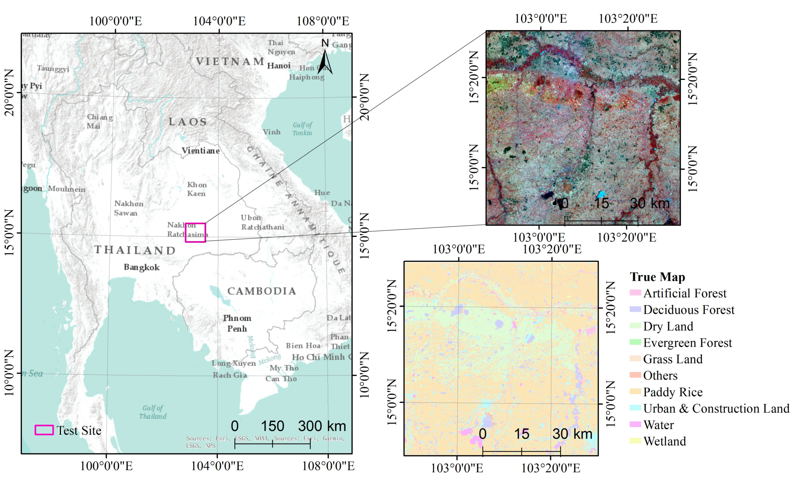
The test site is in the northeast region of Thailand within the Mekong River-Basin, as shown in Figure 1. The location of the site is about 15°00′N and 103°00′E, extending to 5843 km2 and including a total of 3000 × 3150 Landsat pixels. The area features a humid tropical monsoon climate with an annual temperature of 18 °C or greater, and an average annual precipitation of 1300–1500 mm. Crops are cultivated and harvested two or three times per year in many areas due to the suitable hydrothermal conditions. The spectral characteristics for crops can vary at different times and locations since the planting period is not limited by a fixed growing season. We created the reference land cover map by manually interpreting Google Earth high-resolution remote sensing images. The collection period of the Google Earth images ranged from January 2015 to February 2016.
Ten types of land cover were identified on the satellite data at the test site, including Artificial Forest, Deciduous Forest, Dry Land, Evergreen Forest, Grass Land, Paddy Rice, Urban & Construction Land, Water, Wet Land, and “Others”. The site is suitable for the study for the plentiful of land cover types.

2.2. Satellite Data

The study mainly used the MODIS time series data and Landsat 8 operational land imager (OLI) data for data fusion. The MODIS data product was retrieved from the online data pool, courtesy of the NASA (National Aeronautics and Space Administration) Land Processes Distributed Active Archive Center (LP DAAC) and the United States Geological Survey (USGS)/Earth Resources Observation and Science (EROS) Center. Specifically, the MOD09Q1 dataset for 2015 was used. MOD09Q1 provides MODIS band 1–2 surface reflectance at 250 m resolution. It is a level 3 composite of MOD09GQ. Each MOD09Q1 pixel contained the best possible L2G observation during an 8-day period as selected on the basis of high observation coverage, low view angle, the absence of clouds or cloud shadow, and aerosol loading. We obtained the two bands of the MOD09Q1 data for Normalized Difference Vegetation Index (NDVI) calculation. In addition, the quality assessment (QA) of MOD09Q1 data was also acquired by the Land Data Operational Products Evaluation (LDOPE) tool courtesy of LP DAAC and EROS, Sioux Falls, South Dakota (https://lpdaac.usgs.gov/tools/ldope_tools (accessed on 16 February 2021)). The 2015 MOD09Q1 contains 46 images in total.
Landsat 8 OLI images of the test site with cloud cover less than 10% were obtained from the United States Geological Survey (USGS) website (https://earthexplorer.usgs.gov/ (accessed on 16 February 2021)). Landsat 8 carried the operational land imager (OLI), including nine bands, among which eight were multi-spectral bands with a resolution of 30 m, and another 15 m panchromatic band with an imaging width of 185 km × 185 km [21].

2.3. Data Preprocessing

2.3.1. NDVI Curve Noise Reduction

The study used an NDVI time series similarity measure from MODIS data for a preliminary fuzzy classification. NDVI gives an indication of the photosynthetic activity of the vegetation and is calculated as the difference between the near-infrared and visible reflectance divided by the sum of the two [22]. Reflectance values in band 1 and band 2 of MOD09A1 and band 5 and band 4 of Landsat 8 were used to calculate separate NDVI values for each product, as shown in Equation (1):
NDVI = ( ρ n i r ρ r e d ) ( ρ n i r + ρ r e d )
where ρ n i r is the reflectance value of the NIR red band of the MOD09Q1 data and Landsat 8 data, and ρ r e d is the reflectance value of the red band.
Atmospheric conditions, geometric errors of the sensors, sub-resolution changes, and other factors may cause noise in the satellite time series [23]. It is necessary to reduce the noise, and a number of satellite time series noise reduction methods have been compared in the literature [24,25]. In this study, we used the adaptive Savitzky–Golay (S–G) filter in TIMESAT software [26] to reduce noise in the MODIS NDVI time series data. The Adaptive Savitzky–Golay filtering replaces each data value y i , i = 1,…, N by a linear combination of nearby values in a window:
j = n n c j y i + j
where c j is the weight of the ith NDVI value of the filter, which is replaced by a weighted QA value of the NDVI. The data value y i is replaced by the average of the values in the window. The window width n of the filter size is the half-width of the smoothing window. The index j is the running index of the original ordinate data table.
For better noise filtering, TIMESAT employed QA data decoded from the original HDF (Hierarchical Data Format) MODIS data by the LDOPE tools. Specifically, bit 2-3, the “cloud state”, was used as the reference of the weight in Equation (2) for TIMESAT S–G filtering. The clear data (Bit Comb. 00) was weighted to 1, the cloudy data (Bit Comb. 01) was weighted to 0.5, and the mixed and unset data (Bit Comb. 10 and 11) were weighted to 0.1 in the study. We used a window size of 4 for the filter, adaption strength was set as 2, and the number of envelope iterations was set to 3.

2.3.2. Image Registration

The Landsat 8 OLI image was a Level 1T product. We conducted radiometric calibration and a FLAASH model atmospheric correction with ENVI 5.0 SP3 software. Then, the Landsat 8 OLI data were resampled to 25 m with the nearest resampling technique. Finally, MODIS data were registered by the Landsat 8 image.

3. Method

3.1. Overall Fusion Scheme

Overall workflow of multilevel decision fusion is shown in Figure 2.
The fusion scheme can be described as two phases, namely the fuzzy classification process and the decision fusion process. First, fuzzy classification was performed on the MODIS data based on a time series similarity measure method, while the Landsat data fuzzy classification were based on a nearest neighbor classifier. The Landsat data were also classified based on an object-oriented classification. Second, after obtaining the memberships of the three-level data, confidence was evaluated on both local and global scales. Local confidence reflects the spatial distribution of uncertainty and global confidence reflects the performance of the fuzzy classifiers. Third, memberships of the three-level data, local confidence, and global confidence were combined by a decision fusion rule.
After the decision fusion, fuzzy classification results of the three-level data were combined on the basis of the performance of a single classifier. Classifiers with better performance were weighted more in the fusion phase so that the final result preserved better classification results; thus, improving the classification accuracy. The detailed process and parameter acquisition procedure are as follows.

3.2. Fuzzy Classification and Operation

Unlike many traditional classification models, the so-called soft classification gives belongingness or likelihood to several categories rather than the rough Yes or No set [27]. There are many approaches to using a soft classifier, including the fuzzy set theory or D –S theory. There are also many algorithms to “soften” hard classifiers, such as maximum likelihood classifiers [28]. The degree to which an object belongs, or is likely to be a category, is called membership in the fuzzy set theory. In this section, we first introduce the concept of fuzzy classification, or so-called soft classification, and state the relationship between memberships with the fuzzy sets and some definitions and operations on fuzzy set theory. Then, we will illustrate the specific fuzzy classification method to get the membership value of the Landsat pixel, image object, and MODIS pixel.

3.2.1. Fuzzy Aggregation Operators

If an object or class is fuzzy, the fuzzy concept can be introduced to classification. The fuzziness of an object may be caused by many factors, such as mixed pixels, limited feature space, or the spectral similarity between intra-classes [29,30].
To better understand the max–min combination operator, we first introduce some basic notions of fuzzy sets and common aggregation operators used in contextual literature.
A fuzzy set F in a reference set U is characterized by a membership function μ F where μ F : U [ 0 , 1 ] . μ F = 0 means that μ is definitely not a member of F, and 0 < μ F < 1 means that μ is partially a member of A. F and G are two fuzzy sets in U with membership functions μ F and μ G [31]. Several operators can be used for spatial data fusion, such as tnorms, tconorms [32], and mean-like operators, such as the Choquet integral and Ordered Weighted Averaging (OWA) operators [33,34]. The fusion operators including the decision operator, combination operator, and cut operator are based on the classical fuzzy set operations. These operations will serve at the fusion scheme in this paper.
Based on the conflict between sources, the compromise combination operation is defined as:
C ( μ F ( x ) , μ G ( x ) ) = sup x min ( μ F ( x ) , μ G ( x ) )
More flexible combination operators adapted to the context have been proposed, such as the prioritized fusion operator [2,35]:
μ ( x ) = min ( μ F ( x ) , max ( μ G ( x ) , 1 C ( μ F ( x ) , μ G ( x ) ) )
μ ( x ) = max ( μ F ( x ) , mix ( μ G ( x ) , C ( μ F ( x ) , μ G ( x ) ) )

3.2.2. Nearest Neighbor Classification

The nearest neighbor (NN) classifier is the most commonly used fuzzy classification method among supervised classification methods. We chose the NN classifier rather than other fuzzy classifiers for the classification of Landsat data because of the convenience to perform multi-resolution segmentation with eCognition Developer software at the same time. To apply NN classification to Landsat pixel classification and object classification, any other fuzzy classifiers can be operated as pre-classifiers for Landsat pixel and object layer classifiers. The same applies to the time series data. We focused on the improvement of the pre-classifiers rather than the pre-classifiers themselves. The NN classification is based on minimum distance in a NN feature space where the training data are constructed by spectral, shape, or texture feature values. The distance in the NN feature space is decided by a simple Euclidean distance (ED) function. The distance function is shown in Equation (6):
d ( x , y ) = ( i = 1 m ( x i y i ) 2 ) 1 / 2
where d ( x , y ) is the ED of samples to be classified in the NN feature space. The data are more similar to the samples when the ED is smaller. The Euclidean distances provide a chance to range the feature values into fuzzy membership values between 0 and 1.

3.2.3. Image Object Classification

The goal of the middle level in the fusion scheme is to connect the MODIS pixel with the Landsat pixel by the segmented image objects. The advantage of including an object level decision is that the object features contain more information, such as neighborhood information and texture information, for the fuzzy classification. In addition, the object level contains a stack of homogenous pixels that are more reasonable for fusing with the MODIS pixels.
The image segmentation is based on multi-resolution segmentation (MRS) performed on the eCognition platform. The segmentation is confined to MODIS pixels, as illustrated in Figure 2. The MRS in the eCognition platform uses five parameters to control the segmentation result, namely the scale, shape, color, compactness, and smoothness parameters. The segmentation scale, which controls the size of resultant polygons, is the most critical parameter. A good segmentation will produce a balance between polygon size and the homogeneity within an object and heterogeneity between objects. The shape and color parameters define the weight that the shape and color criteria should have when segmenting the image. The higher the value of the shape, the lower the influence of color on the segmentation process. For the compactness and smoothness criteria, the higher the weight value, the more compact image objects may be. We set the value of the scale parameter to 40, shape value to 0.3, and compactness value to 0.5, according to an experiment on the test site. Note that different test sites should have different segmentation parameter values. The operation of the image segmentation guaranteed the registration among three layers, as shown in Figure 3:
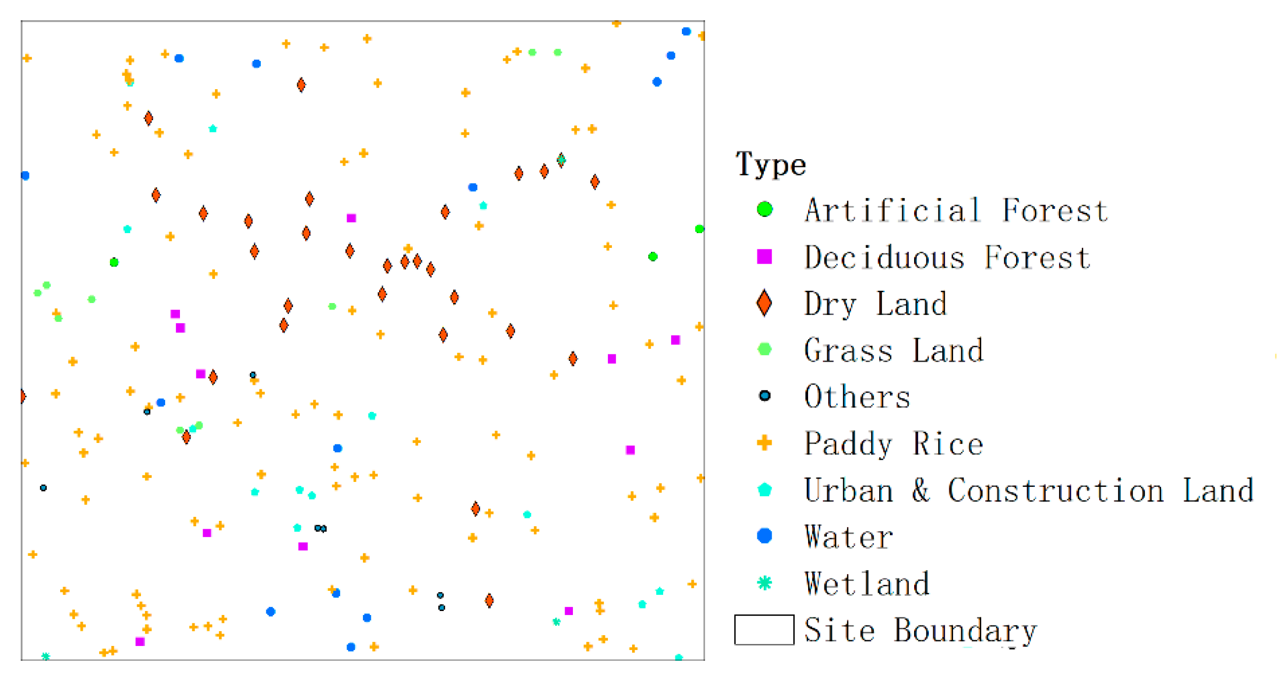
After the segmentation, the objects were classified via sample points. The fuzzy classification process was also performed in the eCognition software. The object information, including the spectral, texture, shape, and difference with neighbor objects were input in a NN feature space for the training of samples. Figure 4 shows the distribution of sample points collected on the reference map to perform the NN classification for the Landsat object level and Landsat pixels.
Finally, the fuzzy classification was performed via the NN classifier, producing memberships of each class.

3.2.4. Time series Similarity

Temporal trajectory analysis is able to exploit temporal patterns in multi-temporal sequences, and time series similarity is an important measure in temporal trajectory analysis [36]. Vegetation usually shows a seasonal temporal trajectory driven by plant phenology [37]. The vegetation index (VI) derived from satellite data has proven vital in detecting vegetation growth conditions. Apart from detecting vegetation, other LC types have also proved to be distinguishable via VI [38]. Hence, the VI time series similarity measure is a powerful method for land cover classification. The ED method time series similarity algorithm has proved to be a simple but effective method to measure time series similarity, and in this article, the ED method was used for the NDVI time series similarity measure. According to the Linear Spectral Unmixing theory, the VI time series is likely to present the dominant LC types. When the landscape is heterogeneous, the VI time series is similar to the average of the LC type VI time series. Membership of MODIS data can be determined by the similarity between each pixel’s VI time series and the reference LC VI time series.
The first step is to build the MODIS NDVI time series. Assume there are N pixels in an image and M layers of MODIS NDVI imagery obtained over a year in chronological order beginning with the first day of the year. Each pixel has two attributes, its coordinates (x, y) and an NDVI sequence defined as: S m = { ( ( x q , y q ) , V I q l ) ,   q = 1 , , N ; l = 1 , , M } , where ( x q , y q ) are the coordinates of each pixel; V I q l are the NDVI values in each layer of MODIS time series data. Usually, the 8-day composite MODIS data have 46 layers, and the value M equals 46. Second, pick the reference time series of each land cover. Because of differences in reflectance, LC types have different VI time series shapes. The standard VI time series is derived from the pure pixels in satellite images or the ground truth data. The standard VI time series serves as a reference curve and compares the similarity with each pixel’s VI time series by ED. Third, calculate similarity between pixels’ VI time series and the reference VI time series, according to the principle of ED, which is the cumulative distance of the corresponding pointwise values on two curves (Equation (7)):
ED = l = 1 M abs ( VI 1 l VI 2 l )
where ED is the Euclidean distance between curve VI 1 l and VI 2 l , and M is the number of points on the curves. Finally, the normalized memberships are obtained using the ED. The smaller the ED value is, the more similar the two curves are. To constrain the value to [0,1], the Euclidean distance of each pixel to a certain land feature’s standard NDVI time series was normalized according to Equation (6) as the normalized Euclidean distance (NED). Finally, the memberships of MODIS data were obtained by the value 1-NED. Equation (8) is the calculation of NED.
NED = ( ED min E D ) / ( max E D min E D )

3.3. Uncertainty & Decision

3.3.1. Pointwise Global

The core class decision method adopts the compromise combination developed in [2] by Fauvel and Benediktsson. We will briefly review the method and explain its usage in the three-layer fusion scheme of this paper. It was assumed that when a membership is “reliable”, it has low fuzziness because a reliable fuzzy set should have a membership significantly higher than the others. On the contrary, when the membership values in a membership are close to each other, the classifier is “unreliable”. The pointwise accuracy can be measured by the fuzziness of a membership (fuzzy set).
Here, we take the research result in [39] as the measurement of fuzziness, which is similar to the description in [3] of a fuzzy set F defined by:
H α QE ( μ F ) = 1 n 2 2 α i = 1 n μ F ( x i ) α ( 1 μ F ( x i ) ) α
where the parameter α is 0.5 in the paper by Löw et al. [3]. We took this parameter as well.
To normalize the effect of weights on different fuzzy sets, in the next step, each fuzzy set was weighted by:
{ ω i = k = 0 , k i m H α QE ( μ F ) ( m 1 ) k = 0 m H α QE ( μ F ) i = 0 m ω i = 1
where E v ( μ k ( μ i ) ) is the degree of fuzziness of source k and m is the number of sources. The value of ω i is close to 1 when a source has a low degree of fuzziness.

3.3.2. Global Accuracy

The local context of uncertainty of the membership can be adopted as one hand of the uncertainty measure. Most decision fusion schemes take the “global accuracy” of the membership as fusion weights. The global accuracy means the classification accuracy by each classifier on the whole image. The global accuracy can be a priori knowledge, but is usually obtained from a posteriori accuracy from the confusion matrix. The class-wise measure of accuracy ( C A i ) can be defined by Equation (11):
C A i = 2 p r i t p i p r i + t p i
where t p i is the true positive rate (TPR), which gives the proportion of samples classified into class i among all samples, which truly have class i, and p r i the precision, which gives the proportion of samples that truly have class i among all samples classified as class i.
Because the MODIS data classification accuracy is highly related to the area proportion, the global accuracy of MODIS data should be added with an area factor ( A p | p = 1 , 2 , 3 , , 10 ) , which is the accuracy of the graded area proportion, the proportion of which is (10, 20, 30, …, 100)1. Thus, Equation (11) is rewritten as:
CA i p = ( A i p CA i 10 ) / p = 1 10 A i p

3.3.3. Decision Rule

Following the fuzzy sets operation introduced in Section 3.2.1, the decision fusion is given by adapting the local context based on the contextual dependent compromise combination. It was proved that the fusion favors the most reliable source by adapting to the local context:
μ f j ( x ) = max ( m i n ( ω i μ i j ( x ) , f i j ( x ) ) ,   i [ 1 , m ] )
where f i j ( x ) is the global confidence of source (classifier) i for class j, ω i is the local context defined in Equation (8), μ i j is an element of the membership, which denotes a membership value to class j, and m is 2 in our scheme. Here, the average class-wise accuracy ( CA i and CA i p ) introduced in the last paragraph will be used as f i j ( x ) .
Before beginning the fusion operation, the image segmentation presented in Section 3.2.3 was performed to produce the object layer. Then, classifying the MODIS data by the time series similarity measure presented in Section 3.2.4 obtained the membership μ m j . Classifying the Object and Landsat pixel data by the nearest neighbor classifier presented in Section 3.2.2 and Section 3.2.3 with sampling points obtained the memberships μ o j and μ l j . Calculating the pointwise accuracy of the classified data with Equation (12) yielded the MODIS data global classification accuracy f m j ( x ) . The object layer’s global classification accuracy f o j ( x ) and the Landsat pixel layer’s global classification accuracy f l j ( x ) were obtained by Equation (11) with sampling points.
In the fusing phase, the local confidence was first obtained by Equation (9) and Equation (10). The local confidence of MODIS membership, object membership and Landsat membership were denoted as ω m , ω o , and ω l . The final fusion method is shown in Equation (14):
μ m o l j ( x ) = max ( m i n ( ω m μ m j ( x ) , f m j ( x ) ) , m i n ( ω o μ o j ( x ) , f o j ( x ) ) , m i n ( ω l μ l j ( x ) , f l j ( x ) ) )

4. Result

Following the fusion schemes and the detailed steps, we tested our fusion method in the test site. Sample points were collected to train the nearest neighbor classification samples and a standard NDVI time series was obtained. The true classification map was obtained by manually interpreting Google Earth high-resolution remote sensing images of the region (dated from January 2015 to February 2016). The classification accuracy was compared with (1) classification results of using the MODIS and Landsat data without decision fusion; (2) decision fusion results using the MODIS and Landsat data by the fusion rule of our scheme; and (3) the selected results of decision fusion, weighted sum fusion [7], and fuzzy classification result of Landsat and MODIS data.

4.1. Reference NDVI Time Series

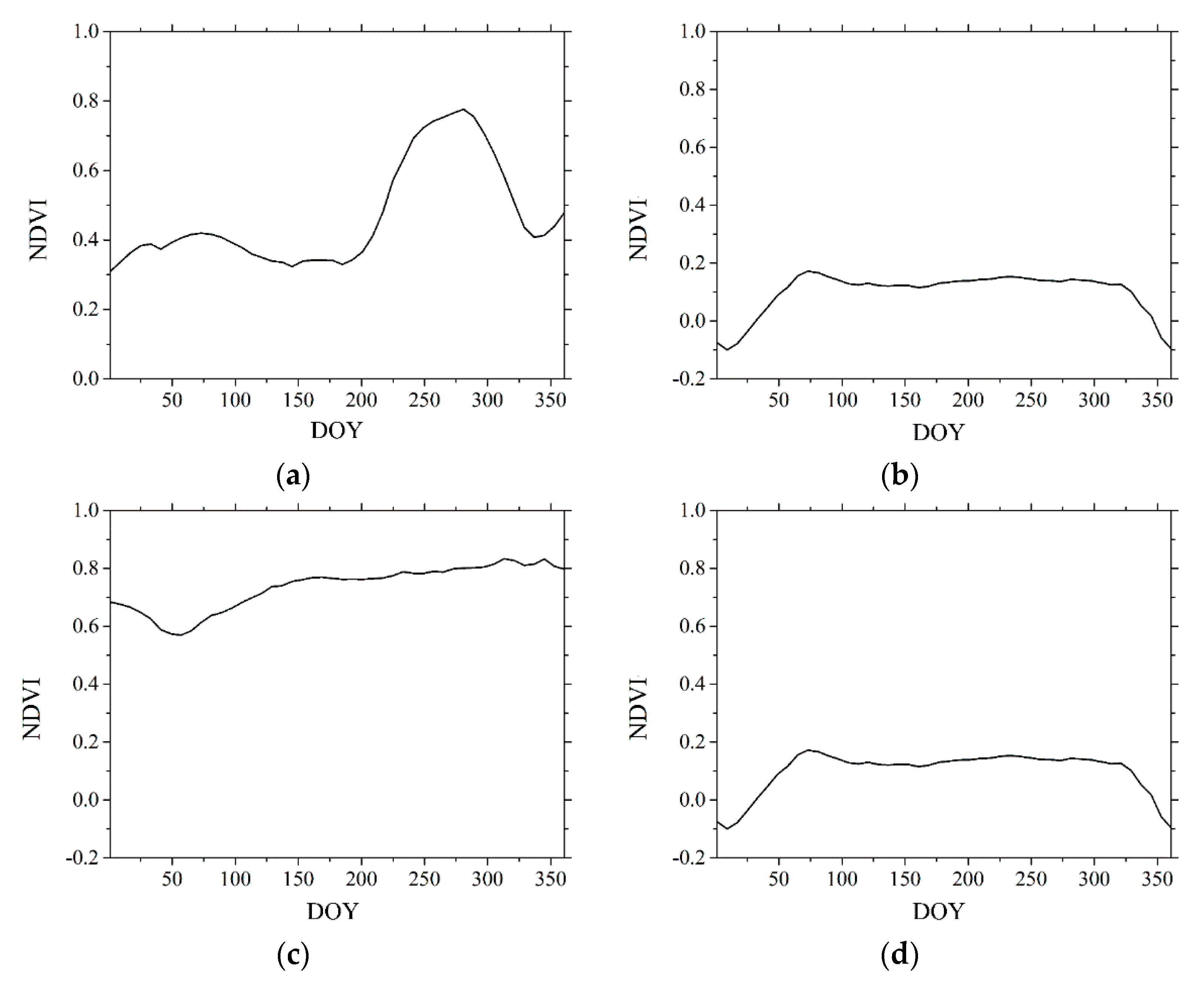
The land cover types have different VI time series shapes due to the differences in reflectance. The standard VI time series was derived from the reference map (Figure 5).

4.2. Membership Value

The Euclidean distance-based similarity measure was applied to classify the MODIS data. Using the nearest neighbor classifier for the classification of Landsat 8 OLI data, we obtained the membership values of the 10 typical land features for the MODIS and Landsat satellite data, as shown in Figure 6. For succinctness, we only illustrate the membership of paddy rice.

4.3. Weighting Factor

Although the MODIS data classification accuracy was generally lower than the classification results of the object or the Landsat pixels, the classification accuracy was high relative to landscape heterogeneity. Using Equation (9) and Equation (10) to calculate the global accuracy of MODIS data, as shown in Table 1, the accuracy generally increased when the image object was larger, which denotes more homogeneity in the landscape. The classification accuracy of the MODIS-classified LC classes was lower than the Landsat data. However, the accuracy of MODIS-classified data was more reliable when the area occupation of the image objects was larger.

4.4. Land Cover Mapping and Accuracy Assessment

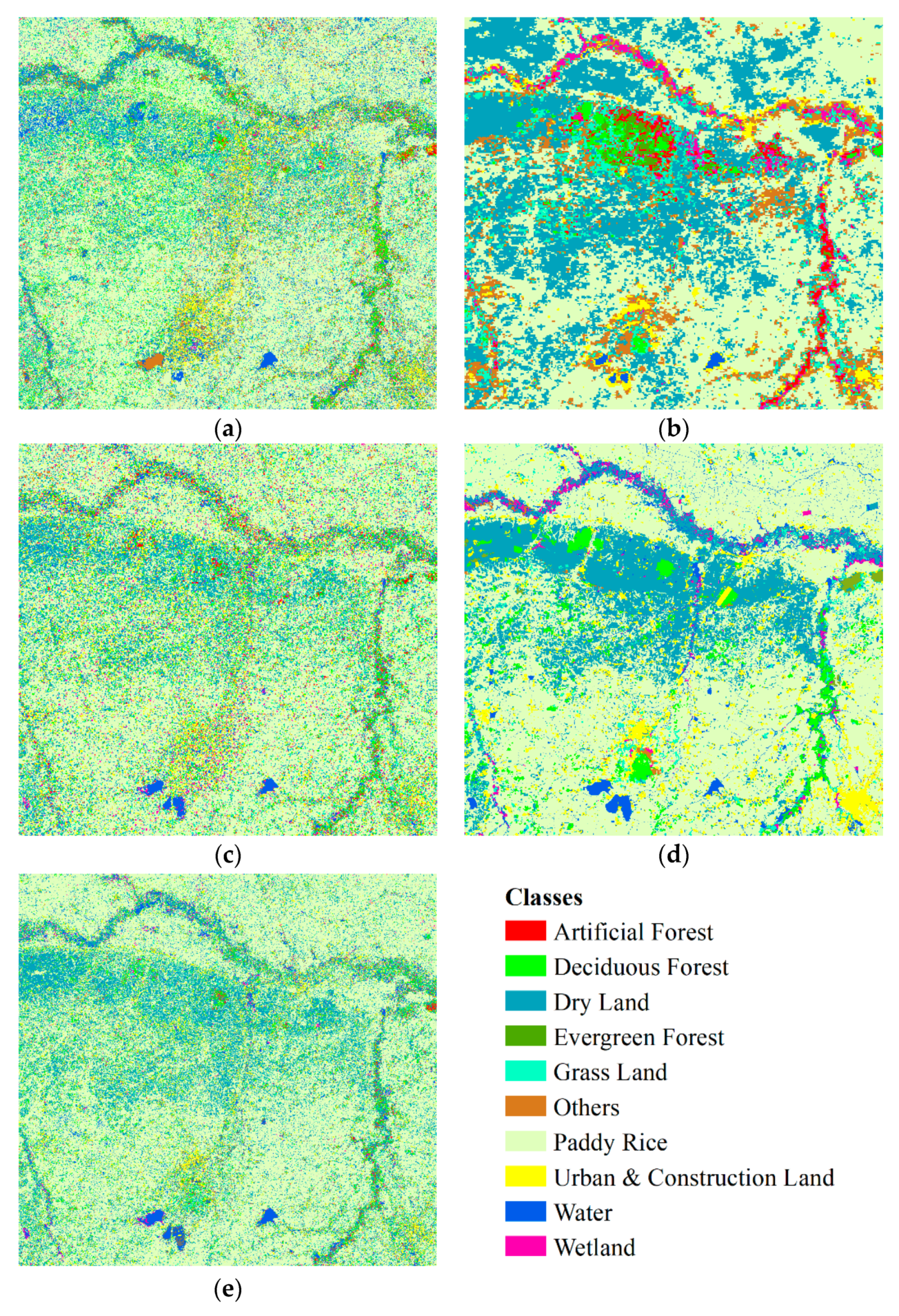
Figure 7 shows the Landsat pixel, object, and MODIS time series classification results by NN and ED classifiers; the real classification image by auto-manual interpretation; and the fused classification image.
Following the fusion scheme, the MODIS data were first classified using the ED fuzzy classifier. The image objects (Obj.) produced by segmentation and the Landsat pixel (LP) was classified using the NN classifier and expressed as NNO and NNP. The final classification results were compared with the fuzzy classification results from mono-source data, namely the MODIS classification results, the Landsat pixel based fuzzy classification, and the image object-based fuzzy classification. The result was also compared with the weighted sum (WS) fusion results. We will refer to our fusion scheme as the three-layer decision fusion (TLDF) for clarity. Indicators included the class-wise accuracy produced by the confusion matrix as well as the overall accuracy (OA) produced by each classification result. We used CA i in Equation (11) to evaluate the classification accuracy of each class type. The comparison results are shown in Table 2.
The weighted sum approach fuses multi-source data by weighted average of the membership values using Equation (15):
μ m o l j ( x ) = ( ω m μ m j ( x ) f m j ( x ) + ω o μ o j ( x ) f o j ( x ) + ω l μ l j ( x ) f l j ( x ) ) / 3
As shown in Table 2, the three-layer decision fusion obtained the highest overall classification accuracy. It improved the MODIS data classification accuracy by 8% and improved the Landsat classification accuracy by more than 5%. The LC types that are highly related to phenology patterns, such as Paddy Rice and Dry Land, had higher accuracy after fusion than the Water, Artificial Land, and Others. The accuracy was close to the highest accuracy of mono- or multi-source classifications. Finally, the classes of Water and Artificial Land had higher classification accuracy after the fusion scheme of our method because of its ability to preserve detailed information.
The results of the first test site illustrate the better performance of the three-layer fusion scheme. Although the best classification accuracy was not obtained by the three-layer fusion scheme for every LC type, it was able to balance the area proportions of the LC types with multi-source classification accuracy.

5. Discussion

Several fusion algorithms have been proposed in previous research to improve the spatial resolution of MODIS data by combining Landsat data at the pixel level. In contrast, the key point in the framework presented in this paper lies in combining the useful information from different data by fusing them at the “decision-level.” There are studies focusing on the fusion of MODIS and Landsat data in the decision-level [40,41]. The difference between our work and others is that we used spatial distribution of the uncertainty in the fusion scheme. In our previous work, we analyzed MODIS 8-day NDVI data classification accuracy with respect to land heterogeneity and showed that MODIS 8-day NDVI data achieve a higher classification accuracy when the land cover is more homogenous [42]. Consequently, when the land cover within a MODIS pixel is homogenous, the information extracted with MODIS 8-day NDVI data are more reliable. Although MODIS is useless for small imaged objects, information extracted from Landsat data can be combined with the reliable parts of the MODIS data. With this method, the Landsat data complement the MODIS data and, thus, using both together improves classification accuracy. However, the previous study [42] encountered the problem of detailed information loss. This article improved the fusion result by adding a Landsat-pixel level, which helps preserve the detailed information of the medium-high resolution data. We also compared the result of a multilevel decision rule with the fusion result of our previous method. The study proves that the multilevel decision fusion rule is superior for fusing spatiotemporal remote sensing data.
This study adopted a simple weighted sum membership function combination rule for decision fusion. The main limitation for the weighted sum combination rule is that the production of the membership values with the weighting factor generated by the classification accuracy of MODIS and Landsat data merges locally reliable values with globally reliable values. This combination rule leads to some unsatisfactory results, such as incorrect classifications obtained by fusing two correct classifications of MODIS data and Landsat data. Although imperfect, this combination rule was capable of improving classification accuracy and achieving good performance with the object-based weighting factor the first time we introduced it in the combination of MODIS and Landsat data at the decision level. We chose the weighted sum combination rule because it is simple and easily understood. We suggest introducing the object-based weighting factor to other decision fusion rules to improve classification accuracy, as introduced in [16], in which the authors were able to separate the local uncertainty from the global accuracy. Moreover, the object-based weighting factor that considers land heterogeneity could be introduced into many other combination rules that involve weighting factors.
Theoretically, one precondition of this method is the assumption that the classification accuracy, for some land cover types from Landsat data, is higher than the classification accuracy for imaged objects that occur at lower proportions in a MODIS pixel (Mcq). Moreover, in turn, this method assumes that MODIS classification accuracy with higher proportions is greater than that from the equivalent Landsat classification data. However, during the accuracy assessments for these experiments, we found that the nearest neighbor-based fuzzy classifications of Landsat data were sometimes affected similarly across the spectrum and that the membership values were similar between some land cover types. Consequently, the MODIS 8-day NDVI data could act as a reference correction to the Landsat image classification results—even when neither of the fuzzy classification accuracies from the MODIS or Landsat data were higher than the other. As illustrated in Figure 6, the memberships produced from NN classification were distributed mainly from 0.8 to 1, which is relatively high. Specifically, for most objects, the memberships of two classes were always higher than others and their numerical values were very close, as shown in Figure 6b. In such cases, MODIS acts as auxiliary information as illustrated in Figure 6a, where a final decision could be obtained for paddy rice.
This study uses a decision fusion method to classify land cover. To take advantage of both the high temporal resolution of MODIS data and the moderately-high spatial resolution of Landsat data, we developed a systematic approach based on fuzzy classification and a decision fusion method to integrate these two-remote sensing products. We applied the method to a test site within the Mekong River Basin. The overall classification accuracy from the fused data is higher than the classification results achievable from Landsat images or MODIS images alone, yielding accuracies of 57.3%, 49.2%, and 51.4%, respectively. About 7% of the incorrectly classified classes were rectified by the decision fusion method. This study shows the proposed fusion scheme is promising for improving classification accuracy, particularly for areas where it is difficult to obtain high-quality, high-to-moderate spatial resolution images.

6. Conclusions

This article applied a decision fusion algorithm developed to combine classifiers for the fusion of MODIS and Landsat data to improve classification accuracy. The decision fusion algorithm was developed based on the fuzzy set theory. The fuzzy classification result, presented as memberships to each class, is operated via a compromise combination operation. We applied this fusion scheme to combine the MODIS time series derived classification information with the Landsat data derived classification information. The object layer also derived fuzzy classification information and connected the coarse resolution MODIS data with the fine resolution Landsat data. An improved global accuracy for the MODIS time series data is proposed by adding an area factor to the accuracy.
This approach proved to be useful in combining the complementary information provided by MODIS and Landsat. A test site located in the Mekong River Basin was selected to verify the approach. The overall accuracy of the test improved by about 7%. It was also proven that the three-layer decision fusion accuracy was greater than the MODIS-object two-layer decision fusion accuracy. Comparisons with another fusion scheme, the weighted sum fusion, was also conducted. The fuzzy set theory-based compromise combination method gained a slightly higher classification accuracy than the weighted sum fusion method, but the weighting also considered the pointwise and global accuracies.
Future work can consider the mixed pixel problem between the MODIS and Landsat data. For example, the relationship between membership values that also denote the combined proportion of endmembers in the coarse resolution data.

Author Contributions

Conceptualization, C.H.; methodology, X.G.; software, R.Z.; validation, X.G.; formal analysis, X.G.; investigation, C.H.; resources, X.G.; data curation, C.H.; writing—original draft preparation, X.G.; writing—review and editing, R.Z.; visualization, X.G.; supervision, C.H.; project administration, C.H.; funding acquisition, C.H. All authors have read and agreed to the published version of the manuscript.

Funding

This research was funded by the National Science Foundation of China, grant numbers 41901309, Special Project of Lancang-Mekong River Cooperation of the Ministry of Science and Technology of the People’s Republic of China, Agricultural Resources and Environmental Survey with Information Platform Construction in Lancang-Mekong River Basin, and the CAS “Light of West China” Program and the Youth Talent Team Program of the Institute of Mountain Hazards and Environment, CAS, grant numbers SDSQB-2020000032, Y8R2230230.

Institutional Review Board Statement

Not applicable.

Informed Consent Statement

Not applicable.

Data Availability Statement

The data presented in this study are openly available in [Mendeley Data] at [doi:10.17632/rch6zwbhxn.1].

Conflicts of Interest

The authors declare no conflict of interest.

References

  1. Cihlar, J. Land cover mapping of large areas from satellites: Status and research priorities. Int. J. Remote Sens. 2000, 21, 1093–1114. [Google Scholar] [CrossRef]
  2. Fauvel, M.; Chanussot, J.; Benediktsson, J.A. Decision fusion for the classification of urban remote sensing images. IEEE Trans. Geosci. Remote Sens. 2006, 44, 2828–2838. [Google Scholar] [CrossRef]
  3. Löw, F.; Conrad, C.; Michel, U. Decision fusion and non-parametric classifiers for land use mapping using multi-temporal rapideye data. ISPRS J. Photogramm. Remote Sens. 2015, 108, 191–204. [Google Scholar] [CrossRef]
  4. Pohl, C.; Van Genderen, J.L. Review article multisensor image fusion in remote sensing: Concepts, methods and applications. Int. J. Remote Sens. 1998, 19, 823–854. [Google Scholar] [CrossRef] [Green Version]
  5. Petrakos, M.; Benediktsson, J.A.; Kanellopoulos, I. The effect of classifier agreement on the accuracy of the combined classifier in decision level fusion. IEEE Trans. Geosci. Remote Sens. 2001, 39, 2539–2546. [Google Scholar] [CrossRef] [Green Version]
  6. Jimenez, L.O.; Morales-Morell, A.; Creus, A. Classification of hyperdimensional data based on feature and decision fusion approaches using projection pursuit, majority voting, and neural networks. IEEE Trans. Geosci. Remote Sens. 1999, 37, 1360–1366. [Google Scholar] [CrossRef]
  7. Lee, D.H.; Park, D. An efficient algorithm for fuzzy weighted average. Fuzzy Sets Syst. 1997, 87, 39–45. [Google Scholar] [CrossRef]
  8. Elfes, A. Multi-source spatial data fusion using bayesian reasoning. In Data Fusion in Robotics and Machine Intelligence; Academic Press: Cambridge, MA, USA, 1992; pp. 137–163. [Google Scholar]
  9. Basir, O.; Yuan, X. Engine fault diagnosis based on multi-sensor information fusion using dempster–shafer evidence theory. Inf. Fusion 2007, 8, 379–386. [Google Scholar] [CrossRef]
  10. Zhang, J. Multi-source remote sensing data fusion: Status and trends. Int. J. Image Data Fusion 2010, 1, 5–24. [Google Scholar] [CrossRef] [Green Version]
  11. Zhu, X.; Chen, J.; Gao, F.; Chen, X.; Masek, J.G. An enhanced spatial and temporal adaptive reflectance fusion model for complex heterogeneous regions. Remote Sens. Environ. 2010, 114, 2610–2623. [Google Scholar] [CrossRef]
  12. Hilker, T.; Wulder, M.A.; Coops, N.C.; Linke, J.; McDermid, G.; Masek, J.G.; Gao, F.; White, J.C. A new data fusion model for high spatial-and temporal-resolution mapping of forest disturbance based on landsat and modis. Remote Sens. Environ. 2009, 113, 1613–1627. [Google Scholar] [CrossRef]
  13. Gao, F.; Masek, J.; Schwaller, M.; Hall, F. On the blending of the landsat and modis surface reflectance: Predicting daily landsat surface reflectance. IEEE Trans. Geosci. Remote Sens. 2006, 44, 2207–2218. [Google Scholar]
  14. Wu, M.-Q.; Wang, J.; Niu, Z.; Zhao, Y.-Q.; Wang, C.-Y. A model for spatial and temporal data fusion. J. Infrared Millim. Waves 2012, 31, 80–84. [Google Scholar] [CrossRef]
  15. Wang, J.; Li, C.; Gong, P. Adaptively weighted decision fusion in 30 m land-cover mapping with landsat and modis data. Int. J. Remote Sens. 2015, 36, 3659–3674. [Google Scholar] [CrossRef]
  16. Baek, W.J. Optimal m-ary data fusion with distributed sensors. IEEE Trans. Aerosp. Electron. Syst. 1995, 31, 1150–1152. [Google Scholar] [CrossRef]
  17. Benediktsson, J.A.; Kanellopoulos, I. Classification of multisource and hyperspectral data based on decision fusion. IEEE Trans. Geosci. Remote Sens. 1999, 37, 1367–1377. [Google Scholar] [CrossRef] [Green Version]
  18. Waske, B.; van der Linden, S.; Benediktsson, J.A.; Rabe, A.; Hostert, P. Sensitivity of Support Vector Machines to Random Feature Selection in Classification of Hyperspectral Data. IEEE Trans. Geosci. Remote Sens. 2010, 48, 2880–2889. [Google Scholar] [CrossRef] [Green Version]
  19. Mitrakis, N.E.; Topaloglou, C.A.; Alexandridis, T.K.; Theocharis, J.B.; Zalidis, G.C. Decision fusion of ga self-organizing neuro-fuzzy multilayered classifiers for land cover classification using textural and spectral features. IEEE Trans. Geosci. Remote Sens. 2008, 46, 2137–2152. [Google Scholar] [CrossRef]
  20. Giacinto, G.; Roli, F. Design of effective neural network ensembles for image classification purposes. Image Vis. Comput. 2001, 19, 699–707. [Google Scholar] [CrossRef]
  21. U.S. Department of the Interior; U.S. Geological Survey. MOD09Q1|LP DAAC: NASA Land Data Products and Services. Available online: https://lpdaac.usgs.gov/dataset_discovery/modis/modis_products_table/mod09q1_v006 (accessed on 14 February 2016).
  22. Roy, D.P.; Wulder, M.; Loveland, T.; Woodcock, C.; Allen, R.; Anderson, M.; Helder, D.; Irons, J.; Johnson, D.; Kennedy, R. Landsat-8: Science and product vision for terrestrial global change research. Remote Sens. Environ. 2014, 145, 154–172. [Google Scholar] [CrossRef] [Green Version]
  23. Chen, J.; Jönsson, P.; Tamura, M.; Gu, Z.; Matsushita, B.; Eklundh, L. A simple method for reconstructing a high-quality ndvi time-series data set based on the savitzky–golay filter. Remote Sens. Environ. 2004, 91, 332–344. [Google Scholar] [CrossRef]
  24. Thonfeld, F.; Schmidt, M.; Dubovyk, O.; Menz, G. On the relevance of radiometric normalization of dense Landsat time series for forest monitoring. In Proceedings of the 2015 IEEE International Geoscience and Remote Sensing Symposium (IGARSS), Milan, Italy, 26–31 July 2015; pp. 2665–2668. [Google Scholar]
  25. Hird, J.N.; McDermid, G.J. Noise reduction of ndvi time series: An empirical comparison of selected techniques. Remote Sens. Environ. 2009, 113, 248–258. [Google Scholar] [CrossRef]
  26. Jönsson, P.; Eklundh, L. TIMESATTIMESAT—a program for analyzing time-series of satellite sensor data. Comput. Geosci. 2004, 30, 833–845. [Google Scholar] [CrossRef] [Green Version]
  27. Deli, I.; Çağman, N. Intuitionistic fuzzy parameterized soft set theory and its decision making. Appl. Soft Comput. 2015, 28, 109–113. [Google Scholar] [CrossRef] [Green Version]
  28. Binaghi, E.; Brivio, P.A.; Ghezzi, P.; Rampini, A. A fuzzy set-based accuracy assessment of soft classification. Pattern Recognit. Lett. 1999, 20, 935–948. [Google Scholar] [CrossRef]
  29. Benz, U.C.; Hofmann, P.; Willhauck, G.; Lingenfelder, I.; Heynen, M. Multi-resolution, object-oriented fuzzy analysis of remote sensing data for gis-ready information. ISPRS J. Photogramm. Remote Sens. 2004, 58, 239–258. [Google Scholar] [CrossRef]
  30. Foody, G. Sharpening fuzzy classification output to refine the representation of sub-pixel land cover distribution. Int. J. Remote Sens. 1998, 19, 2593–2599. [Google Scholar] [CrossRef]
  31. Szmidt, E.; Kacprzyk, J. Entropy for intuitionistic fuzzy sets. Fuzzy Sets Syst. 2001, 118, 467–477. [Google Scholar] [CrossRef]
  32. Khaleghi, B.; Khamis, A.; Karray, F.O.; Razavi, S.N. Multisensor data fusion: A review of the state-of-the-art. Inf. Fusion 2013, 14, 28–44. [Google Scholar] [CrossRef]
  33. Yager, R.R. On Ordered Weighted Averaging Aggregation Operators in Multicriteria Decisionmaking; IEEE Press: New York, NY, USA, 1988. [Google Scholar]
  34. Yager, R.R. A framework for multi-source data fusion. Inf. Sci. 2004, 163, 175–200. [Google Scholar] [CrossRef]
  35. Bloch, I. Information combination operators for data fusion: A comparative review with classification. IEEE Trans. Syst. ManCybern. Part A Syst. Hum. 1996, 26, 52–67. [Google Scholar] [CrossRef]
  36. Guan, X.; Huang, C.; Liu, G.; Meng, X.; Liu, Q. Mapping Rice Cropping Systems in Vietnam Using an NDVI-Based Time-Series Similarity Measurement Based on DTW Distance. Remote Sens. 2016, 8, 19. [Google Scholar] [CrossRef] [Green Version]
  37. Lhermitte, S.; Verbesselt, J.; Verstraeten, W.W.; Coppin, P. A comparison of time series similarity measures for classification and change detection of ecosystem dynamics. Remote Sens. Environ. 2011, 115, 3129–3152. [Google Scholar] [CrossRef]
  38. Geerken, R.; Zaitchik, B.; Evans, J. Classifying rangeland vegetation type and coverage from ndvi time series using fourier filtered cycle similarity. Int. J. Remote Sens. 2005, 26, 5535–5554. [Google Scholar] [CrossRef]
  39. Klir, G.J. Where do we stand on measures of uncertainty, ambiguity, fuzziness, and the like? Fuzzy Sets Syst. 1987, 24, 141–160. [Google Scholar] [CrossRef]
  40. Bisquert, M.; Bordogna, G.; Bégué, A.; Candiani, G.; Teisseire, M.; Poncelet, P. A Simple Fusion Method for Image Time Series Based on the Estimation of Image Temporal Validity. Remote Sens. 2015, 7, 704–724. [Google Scholar] [CrossRef] [Green Version]
  41. Swathika, R.; Sharmila, T.S. Image fusion for MODIS and Landsat images using top hat based moving technique with FIS. Clust. Comput. 2019, 22, 12939–12947. [Google Scholar] [CrossRef]
  42. Guan, X.; Liu, G.; Huang, C.; Liu, Q.; Wu, C.; Jin, Y.; Li, Y. An Object-Based Linear Weight Assignment Fusion Scheme to Improve Classification Accuracy Using Landsat and MODIS Data at the Decision Level. IEEE Trans. Geosci. Remote Sens. 2017, 55, 6989–7002. [Google Scholar] [CrossRef]
1
Example: the class-wise accuracy of LC type A is 0.37. A i p = { 0.54 , 0.58 , 0.57 , 0.59 , 0.64 , 0.73 , 0.76 , 0.83 , 0.83 , 0.89 } . Then, the area of an object occupies 32.2% in a MODIS pixel. Then CA i p = 0.57 0.37 10 14.4 = 0.146 . This means that when the object occupies 32.2%, the classification accuracy of LC type A is 0.146.
Figure 1. Location of the test site.
Land 10 00208 g001
Figure 2. Overall Fusion Scheme of the method.
Land 10 00208 g002
Figure 3. Image segmentation restricted in MODIS pixels.
Land 10 00208 g003
Figure 4. Sample points for nearest neighbor (NN) classifier.
Land 10 00208 g004
Figure 5. Normalized Difference Vegetation Index (NDVI) curves selected by Sample 2, which is a pure-pixel site. The reference NDVI time series is succinctly displayed with only four classes: (a) is the paddy rice annual NDVI curve; (b) water annual NDVI curve; (c) is the deciduous forest annual NDVI curve; and (d) is the evergreen forest annual NDVI curve.
Land 10 00208 g005
Figure 6. Possibility maps: (a) shows the membership values for the paddy rice class given by the Euclidean-based similarity measure from the MODIS NDVI time series while (b,c) show the class probability of the paddy rice class obtained by the nearest neighbor-based fuzzy classification of Landsat data at the object level and the pixel level, respectively.
Land 10 00208 g006
Figure 7. (a) Land cover (LC) map with Landsat pixel using NN classifier, (b) LC map with MODIS pixels using Euclidean distance (ED) classifier, (c) LC map with Landsat objects using NN classifier, (d) true LC map, (e) LC map using the fusion scheme of this paper.
Land 10 00208 g007
Table 1. Graded area’s global accuracy of MODIS data.
Area GradeAccuracy/LC TypesGS 1EF 2AL 3DL 4DF 5OT 6AF 7WL 8WT 9PR 10
Accuracy/graded area8.329.29.554.436.710.418.221.724.373.2
140.56.2 21.9 7.1 40.9 27.6 7.8 13.7 16.3 18.3 55.0
241.96.5 22.7 7.4 42.3 28.5 8.1 14.1 16.9 18.9 56.9
342.66.6 23.1 7.5 43.0 29.0 8.2 14.4 17.1 19.2 57.8
451.37.9 27.8 9.0 51.8 34.9 9.9 17.3 20.6 23.1 69.7
547.97.4 25.9 8.4 48.3 32.6 9.2 16.2 19.3 21.6 65.0
659.99.2 32.4 10.6 60.4 40.8 11.6 20.2 24.1 27.0 81.3
762.39.6 33.7 11.0 62.9 42.4 12.0 21.0 25.1 28.1 84.6
858.39.0 31.6 10.3 58.8 39.7 11.2 19.7 23.5 26.3 79.2
963.49.8 34.3 11.2 64.0 43.2 12.2 21.4 25.5 28.6 86.1
1071.010.9 38.5 12.5 71.6 48.3 13.7 24.0 28.6 32.0 96.4
1 GS—Grass Land. 2 EF—Evergreen Forest. 3 AL—Urban and Construction Land (Artificial Land). 4 DL—Dry Land. 5 DF—Deciduous Forest. 6 OT—Others. 7 AF—Artificial Forest. 8 WL—Wetland. 9 WT—Water. 10 PR—Paddy Rice.
Table 2. Test accuracy of C A i and overall accuracy.
Classification Method/LC TypeEDNNONNPWSMODIS-ObjectTLDF
GS 18.35.75.36.54.75.9
EF 229.248.253.742.140.341.2
AL 39.516.322.68.710.39.5
DL 454.436.231.756.655.656.8
DF 536.758.142.515.020.322.7
OT 610.47.96.30.00.010.1
AF 718.23.2.06.20.00.05.2
WL 821.78.48.118.212.713.3
WT 924.329.722.526.126.828.6
PR 1073.274.573.776.977.377.6
O.A. 1149.252.751.454.655.257.3
1 GS—Grass Land. 2 EF—Evergreen Forest. 3 AL—Urban and Construction Land (Artificial Land). 4 DL—Dry Land. 5 DF—Deciduous Forest. 6 OT—Others. 7 AF—Artificial Forest. 8 WL—Wetland. 9 WT—Water. 10 PR—Paddy Rice. 11 O.A. —Overall Accuracy.
Publisher’s Note: MDPI stays neutral with regard to jurisdictional claims in published maps and institutional affiliations.