Abstract
Sustainable forest management needs to address biodiversity conservation concerns. For that purpose, forest managers need models and indicators that may help evaluate the impact of management options on biodiversity under the uncertainty of climate change scenarios. In this research we explore the potential for designing mosaics of stand-level forest management models to address biodiversity conservation objectives on a broader landscape-level. Our approach integrates (i) an effective stand-level biodiversity indicator that reflect tree species composition, stand age, and understory coverage under divergent climate conditions; and (ii) linear programming optimization techniques to guide forest actors in seeing optimal forest practices to safeguard future biodiversity. Emphasis is on the efficiency and effectiveness of an approach to help assess the impact of forest management planning on biodiversity under scenarios of climate change. Results from a resource capability model are discussed for an application to a large-scale problem encompassing 14,765 ha, extending over a 90-years planning horizon and considering two local-climate scenarios. They highlight the potential of the approach to help assess the impact of both stand and landscape-level forest management models on biodiversity conservation goals. They demonstrate further that the approach provides insights about how climate change, timber demand and wildfire resistance may impact plans that target the optimization of biodiversity values. The set of optimized long-term solutions emphasizes a multifunctional forest that guarantees a desirable local level of biodiversity and resilience to wildfires, while providing a balanced production of wood over time at the landscape scale.
1. Introduction
Forests harbor over half of all terrestrial biodiversity and generate ecosystem services essential to the humankind [1]. Nevertheless, the request for goods and services from forest systems has increased constantly [2]. Consequently, forest management is multifaceted [3] and it targets the supply of a wide range of ecosystem services (ES) that include biodiversity conservation [4,5]. Forest biodiversity—the diversity of species within a forest ecosystem—plays a central role in ecosystem functioning and in sustaining the provision of multiple ecosystem goods and services; that is, the benefits humans obtain from ecosystems [6,7,8,9,10,11].
In this context, forest ecosystem productivity and its multifunctionality are intricately linked with underlying biodiversity [12,13,14]. However, biodiversity has been steadily decreasing worldwide, thus calling for the implementation of conservation policies to mitigate this trend [15]. Forest managers are faced with the need to tackle biodiversity conservation in the management of planted forests. Nevertheless, changes in ecological conditions are expected to impact the functioning of forest ecosystems and affect the provision of all ecosystem services [16,17]. An accurate estimate of biodiversity will assist forest actors to design plans that in the long term increase the adaptability of forests to future environmental changes [18].
Forest management planning needs to define and distribute over time and space silvicultural practices in order to increase the supply of market goods and services while mitigating negative impacts of climate drivers and disturbance regimes on biodiversity [19]. This may encompass the modification of thinning regimes, rotation lengths, and species composition as well of the structure of forest stands [20,21,22]. Brunette et al. [23] reported that the rise in tree species diversity is an appropriate option for preserving ecosystem functioning under climate change, while Seibold et al. [24] showed that boosting the share of broadleaf species in the landscape can benefit forest biodiversity. Other authors have recommended the design of landscapes where specific areas are left uncut or retained to provide wildlife habitat (e.g., green-tree retention, GRT) [25,26,27,28] as a relevant biodiversity-oriented management response to forest biodiversity decline in managed landscapes [29,30]. More recently this approach has been popularized as variable retention (VR). It may encompass further the allocation of areas to multi-aged stands [31], the increase of old-growth areas and its distribution to achieve greater continuity and structural complexity [29,32]. Shea et al. [33] showed how this strategy is effective in conserving biodiversity at landscape-level, especially when there are moderate levels of fragmentation [34,35]. Augustynczik et al. [36] and Ezquerro et al. [20] demonstrated the application of this approach to address biodiversity conservation in landscape-level management. Notwithstanding, practical applications of these adaptation practices are still scarce and/or recent [37], hampering the development of reliable information to assist forest management planning and stakeholders’ decision-making processes.
Nevertheless, the definition of biodiversity indicators is influential to explicit conservation objectives in forest management planning and to help assess the impact of alternative landscape mosaics on biodiversity. The literature reports, since the late eighties, the use of a wide range of indicators [20,29,32,38,39,40]. For example, some authors report the use of the amount of deadwood [39,41,42,43]. Kouki et al. [34] and Augustynczik and Yousefpour [38] highlighted the importance of increasing the amount of deadwood in European forests to improve the habitat of threatened species. In general, the selection of biodiversity indicators for use in management planning must consider its practicality, cost-effectiveness and environmentally meaningfulness [44]. Moreover, the selection must consider the availability of models for projecting the indicator value over the management planning temporal horizon.
In this context, indicators that may be easily measured and for which projection models are available appear to be the most practical. The literature reports the need to identify indicators that reflect tree species composition and vertical structural diversity (e.g., diameter heterogeneity, tree height, basal area, stand age, and canopy cover), including the shrub layers and those that are environmentally significant and suitable for different types of managed forests [39,45,46,47,48,49,50,51,52]. Understory vegetation comprises one of the most significant elements of biodiversity within plantations and is often the sole best predictor of animal diversity (e.g., [53]).
Effectively addressing biodiversity concerns in forest management planning requires further the development of methods that may provide information about the impacts of alternative landscape mosaics on the values of biodiversity indicator, across a wide diversity of forest types and biogeographical–socio-economic conditions and other relevant forest ES. This is influential to compare planning strategies and to propose efficient solutions. The literature reports several alternatives and silvicultural options to integrate biodiversity and wood production in forest management [26,54]. The literature reports several methods to optimize wildlife habitat and biodiversity conservation management. Thompson et al. [55] pioneered the use of linear programming (LP) to integrate wildlife and timber objectives while Hof and Joyce [56] and Hof et al. [57] built mixed-integer and integer programming models to facilitate this integration. Other authors reported the use of heuristics to address wildlife habitat concerns [58]. Mathematical programming approaches have been developed further to address reserve selection problems [59,60,61]. More recently, Marto et al. [62] used a combination of Pareto frontier approaches [63] and multiple attribute techniques [64] to address biodiversity objectives in a multiple-objective decision-making framework. The reader is referred to Ezquerro et al. [65] for a comprehensive review of methods to integrate biodiversity in forest management planning. However, a comprehensive understanding of how silvicultural treatments affect biodiversity indicators and how these effects interrelate with climate change and other ES outcomes in managed forests is still limited. Moreover, despite the large body of literature dealing with the ecological aspects of biodiversity-oriented models, the estimation of practical and quantitative indicators for application in the framework of landscape-level management planning Mediterranean managed forests remain unexplored.
We address this gap by developing an approach that integrates a biodiversity-oriented management indicator that reflect the interaction between tree species composition, stand age, and understory coverage, under scenarios of divergent climate conditions, and linear programming-based (LP) optimization techniques. We use indicators addressing biodiversity at the stand and forest management unit scales. Forest management at the landscape scale addressing, for example, issues related to habitat fragmentation and connectivity are not addressed by the present study. After describing the approach, findings are discussed for an application to a large-scale problem in Northwestern Portugal (Vale do Sousa) encompassing 14,765 ha classified into 1373 stands, for a 90-year planning horizon across two local-climate scenarios. We examine the potential of the approach to help assess the quantitative impact of both stand and landscape-level forest management models on biodiversity. Further, we analyze the insights provided by the approach on how climate change may impact plans that target the optimization of landscape-level biodiversity values.
2. Materials and Methods
2.1. The Vale de Sousa Forested Landscape. Stand-Level Forest Management Models
Vale do Sousa case study area (VA_CSA) is located in Northwestern Portugal and spans three districts: Paiva, Paredes, and Penafiel (Figure 1). It is a forested landscape that covers 14,765 ha and encompasses 1373 stands (Figure 1), with 360 forest owners as ZIF members (ZIF—Forest Intervention Zones). The ZIF was designed to overcome the main bottlenecks in the implementation of forest management models (FMMs), namely at landscape-level management planning: small scale and property fragmentation in multiple blocks, being mostly privately owned [66]. A local forest owners association is the major actor responsible for developing the landscape management planning between two areas of joint collaborative management: ZIF of Entre-Douro-e-Sousa (north of the Douro river) and ZIF Paiva (south of the Douro river) and aims at exploring its potential to address biodiversity conservation concerns. The planning horizon includes nine 10-years periods. Management planning must be in accordance with the Regional Programme for Forestry Planning in Entre Douro e Minho (PROF EDM) which defines specific rules at the regional-level, to promote and guarantee the production of goods and services and the sustainable development of these forests [67], http://www.fao.org/faolex/results/details/en/c/LEX-FAOC183340.
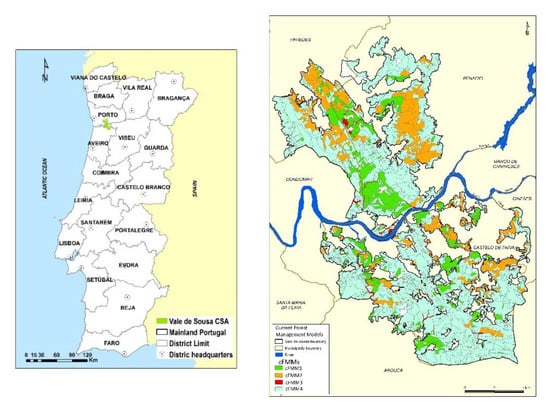
Figure 1.
Vale de Sousa Case study area (Vsousa_CSA) location in Portugal, with 1373 management units (MU) and Current stand-level forest management models (cFMMs).
Current stand-level forest management models (cFMMs) in VA_CSA include eucalypt (Eucalyptus globulus Labill) plantations that are either managed as mixed stands with maritime pine (Pinus pinaster Aiton) (cFMM1 and cFMM2) or as pure stands (cFMM4). These cFMMs extend over 99% of the area. Hardwoods mostly chestnut (Castanea sativa) (cFMM 3) occupied 1% of the remaining area (Figure 1). Several silvicultural treatments were considered under each cFMM (Table 1).

Table 1.
Forest species, current and alternative forest management models and corresponding prescriptions at Vale do Sousa case study area.
The forest owner’s association wants to explore the possibility of species conversions and of using alternative stand-level forest management models (aFMMs) in their planning exercise. Specifically, they consider four aFMMs as driven by surveys of a heterogeneity of stakeholders in VS_CSA [68]. These stakeholders cover a wide range of interests, from commercial private forest owners to environmental NGOs. aFMM’s focus is on native tree species, increasing sustainable and ecological good and services, and creating fire-resistant landscapes (Table 1). In addition, aFMM8 involves a considerable interest in alluvial ecosystems where nature conservation and watershed management are most important.
The research has been conducted following three steps:
- (1)
- A specific growth model to estimate forest growth dynamics under divergent climate conditions have been applied.
- (2)
- The potential biodiversity benefits as a proxy indicator for eight FMMs at stand-level and five fuel treatments (no fuel treatment, annually fuel treatment, each 5-years, and 10 and 15-years) has been computed.
- (3)
- A landscape-level LP-RMC was extended to integrate a biodiversity-oriented forest management indicator taking into account wood provisioning and wildfires reduction, and two local climate scenarios, namely, Business as usual (BAU) and REF (high climate forcing with a RCP 8.5) to evaluate how the essential increase in biodiversity supply can be accomplished through alternative forest models.
2.2. Climate Change Scenarios
Two local-climate scenarios for each FMMs were considered: Business as usual (BAU—considering climate conditions would remain the same) with 13.8 °C and 1194 mm in local mean annual air temperature and local mean annual precipitation, respectively [69]; and “Reference” (REF—high climate forcing) compatible with its respective Representative Concentration Pathway (RCP 8.5) resulting at 2106 in a temperature increase of 2.35 °C and rainfall increase of 193 mm. Local climate change conditions with expected increments in the mean annual temperature, forecast a higher frequency of extreme events, such as severe wildfires and droughts. In addition, an increase in the number and intensity of extreme rain events in the local-climate scenario RCP8.5 will have consequences in this region, including the exacerbate of soil erosion risks highlighted the susceptibility of the CSA to rain erosivity [70].
For REF and BAU scenarios, both the mean annual air temperature and the annual precipitation estimates were generated consistently for the CSA location, based on the climate model KNMI_RACMO22E [71], using the Clipick online tool—climate change web picker weather application [72]; http://www.isa.ulisboa.pt/proj/clipick/. For the REF scenario, data generated from 2017 to 2106 are the basis for assessing the impact of climate conditions on the provision of biodiversity levels by the Linear Programming-Resource capability model (LP-RCM) [73]. For the BAU scenario, the 1981–2010 data set was retrieved and repeated up to 2016.
2.3. Forest Growth Simulations
Forest development for BAU scenario was assessed through specific empirical growth and yield models. Starting with the status of the forests, the models allow to simulate the evolution of different variables ninety years into the future (wood production, biomass, and carbon stocks). The simulations were conducted for 1373 stands where forest inventory data was available. The forest inventory data, including the diameter breast height (dhb, cm), tree height (h, m) and tree density (number of trees per ha, Nt, ha) was used as input. The standsSIM-MD module [74] was used to project stand growth and estimate wood product yields, and to generate stand-level prescriptions for maritime pine (cFMM1, cFMM2 and aFMM5—PINASTER forest model) [75] and eucalyptus (cFMM1, cFMM2 and cFMM4—GLOBULUS forest model) [76] over a 90-year planning horizon. The Castanea sativa (cFMM3) wood production was estimate using the corresponding yield tables [77,78]. For aFMM6 to calculate the wood available an empirical growth and yield model integrated in SimGaliza, a Quercus robur simulator developed in Galicia (Spain) which have soil and climate conditions similar to our CSA was used [79,80]. The SUBER forest model simulator was used to project the growth and production of cork oak stands (aFMM7) [81,82]. It is a growth and yield model at tree-level, presently incorporated in the user—friendly sIMfLOR platform [83]. Regarding aFMM8 structural parameters over time were obtained from Riparian stands National databases [84,85].
For each FMMs the shrub biomass accumulation (Mg. ha−1) under canopy cover was projected according to Botequim et al. [86]. The most frequent shrubs species in the VA_CSA are Adenocarpus argyrophyllus, Cistus ladanifer, Erica spp. or Calluna spp., Quercus lusitanica, Rubus fruticosus, and Ulex spp. In addition, a fuel treatment schedule options (no fuel treatment, 1-year fuel treatment, 5-years, 10-years, and 15-years fuel treatment) was applied over the whole planning horizon. Fuel removal prescriptions are carried out manually or mechanically in the understory vegetation, considering the slope and other site restrictions.
Forest management regimes were then projected to vary in response to REF local-climate scenario. No process-based models might be used to confirm the impact of climate change on tree growth and species suitability. We derived for REF scenario the corresponding climatic variables used as BAU’s output growth simulations. Moreover, the impact of climate change on the trees growth was evaluated according to the findings that are reported in Santos and Miranda [73]. Thus, based on information (averages for the region) from the SIAM Study [87] a percentage in yield under REF’ climate change scenario over the planning horizon was linearly adjusted. Specifically, it was assumed that the yield increased linearly up to 3.52% (cork oak—FMM7) and 4.2% (remaining FMMs) in the main Portuguese forest species in the last year of the planning horizon. Indeed, adjustments to host the temperature changes over 90-years were made to the current values of standing volume and harvested volume (as well as on biometric variables such as h, dbh, standing basal area).
2.4. Biodiversity Management-Oriented Indicators
The approach presented assumes a FMM in which a biodiversity score ranging between 1 and 7 (being “7” the ideal score) increases with shrub cover (e.g., wildlife habitat cover) and changes according to tree composition and forest structure. The criteria used to categorize the biodiversity proxies encompassed the forest species composition (e.g., pine, eucalypt, chestnut, pure pedunculate oak, cork oak, and riparian trees), the stand age, and the site index. The contribution of each species to biodiversity proxies is also scored according to the corresponding age (i.e., time since planting) assigning higher values to higher ages. Older stands provide better habitat for forest species than young stands because of increased spatial and vertical heterogeneity, a better light environment, well-developed soil organic layers, and associated fungal floras [54]. The biodiversity goals should then enable differentiation between tree species of higher or lower importance for biodiversity. In addition, a specific indicator based on shrub biomass quantification as per Botequim et al. [85] was used. The corresponding “biomass” indicator was measured using the calculated biomass (Mg. ha−1) under canopy cover associated with habitat-biodiversity benefits (Table 2). The maximum score for the understory biodiversity refers to the highest availability of cover and habitat for wildlife. If a biodiversity score is equal to “0”, this represents the absence of shrubs under a tree canopy, in turn, the maximum biodiversity score will be achieved with total shrub coverage. Consequently, our approach assumed that increased shrub cover in forest plantation stands, increases habitat heterogeneity and habitat structural diversity, therefore potentially benefiting biodiversity at the species level.
Table 2.
Biodiversity proxies’ indicators used to categorize all FMMs at stand and landscape scale.
In this sense, a final biodiversity score combines tree species proportion with the amount of forest fuel loading shrub cover. Thus, the mixed stands of maritime pine and eucalypts biodiversity score range from less than “1” to more than “3” according to the dominance of eucalypt and pine. Eucalypt pure stands, intensively managed, with relatively limited biodiversity value will be associated to a maximum biodiversity score between “1” and more than “2”. The chestnut biodiversity FMM will score between “3” and more than “4” based on both biodiversity composition and age with a dense understory. For the new aFMMs the pedunculate and cork oak biodiversity score range from “5” to “6”, and finally the riparian systems with a dense understory will be associated to a maximum biodiversity higher than “6”. The set of relevant stand-level FMMs will be evaluated against each of the specific indicators mentioned above (Table 3), using a score of 1–7, being “7” the ideal score. These scores for each year were reported in FMMs rotation.
Table 3.
Species proportion, rotation and minimum values used to define biodiversity scores at stand-scale.
More explanation on the biodiversity management-oriented indicator is presented in Appendix A.
Moreover, these stand-level outcomes are used to define biodiversity scores at the landscape-scale (Equation (1)).
where is the final biodiversity score per management unit (MU), Min is the minimum score per each forest species (S), Max(Rot) is the maximum rotation for each forest species (S), Biom is the amount of biomass per species and management unit; Max (Biom) maximum of biomass across the landscape, Prop is the proportion of species specially for mixed stands (cFMM1 and cFMM2) (Table 3).
2.5. Forest Management Optimization under Biodiversity Conservation
The newly developed biodiversity criteria were integrated into a strategic forest planning model. A Linear Programming (LP) model (BAU—Equations (2)–(25)) aiming to maximize forest biodiversity was designed and allows:
- (i)
- analyzing the provision of biodiversity values under conflicting ES demand scenarios such as timber production and fire resistance, at landscape-level;
- (ii)
- evaluating the impact of site-specific climate change in long-term decisions (90-years);
- (iii)
- evaluating the impacts of alternative forest management models for biodiversity provisions
The biodiversity score used in the optimization models is obtained from equation 1. As mentioned in Appendix A, which is an annual balance of the binomial tree species composition and age rotation and the accumulated biomass for each fuel treatment, further computed in biodiversity score. All possible forest management regimes, as described in Section 2.1 were considered. A total of 250,130 stand-level prescriptions were simulated over the 90-year planning horizon with 10-year periods. Additionally, the set of prescription includes a fuel treatment regime (shrub cover removal) with frequency of 1, 5, 10, or 15-years as well as the option of no fuel treatment. The LP_BAU consists of sets of 25 mathematical equations to estimate the landscape-level provision of biodiversity over the planning horizon, in which prescriptions correspond to the decision variables. The coefficients of the decision variables in each equation describe the contribution of each prescription to the provision of each ES (Table 4). A main scenario that strives to maximize the biodiversity score (solution#1), however, with the addition of a focus on wood production (solution#2) and environmental restrictions with an effort to mitigate the wildfire risk, (solution#3) has been applied. A set of endogenous constraints to guarantee that the area chosen by the model may not exceed the available area in each stand have been included, encompassing 1373 stand area equations (Equation (4)). In addition, constraints following the indications of the forest managers on a minimum of wood production over the 90-year planning horizon (Equation (22)) (defined with a 9 million cubic meters threshold for harvested wood, TWood—Marques et al. [88]) and a maximum 10% fluctuations between consecutive planning periods’ timber harvesting were included (Equation (23)). Further, constraints related to a minimum wildfire vulnerability (wildfire resistance indicator, WRISK > 3—Marques et al. [88]) have been tested (Equation (24)).
Table 4.
Description of sets, variables and data applied in the linear programming (LP)-based optimization model.
Each management unit wildfire resistance was calculated according to the approach described by Marques et al. [89]. The latter considers management-related biometric variables to model wildfire occurrence and damage as well as neighboring stand features that may impact wildfire spread [90]. The resultant stand-level values were averaged for the whole landscape and scaled from “1” to “5”, where 5 represents the highest fire resistance. Inequalities (Equation (25)) set the model’ non-negativity constraints. From the optimal management solutions, we retrieved the prescriptions assigned to achieve a biodiversity conservation goal and provide results-oriented reports on alternative silvicultural models and associated provision of biodiversity.
Afterwards, the effects of the local-climate change scenarios on the provision of biodiversity indicators across a 90-year planning horizon was estimated by the LP_REF under a RCP 8.5 (averages for the region) based on forest growth in Northern Portugal—SIAM national study [87]).
The LP_REF was tested initially by maximizing biodiversity conservation values; than by considering the same LP-formulation with addition of target constraints (Equations (22)–(24). Specifically, the set of constraints ensures that the wood production is at least 9 million cubic meters over the planning horizon with a 10% timber even-flow for the total wood harvested in each period (Equations (22) and (23)). Finally, optimizing biodiversity, maintaining a wildfire resistance greater than 3 (medium vulnerability) (Equation (24)). All LP-problems were read and solved using CPLEX Interactive Optimizer [91].
2.6. LP-RCM Mathematical Formulation
Maximize Z = BIOD
Subject to:
3. Results
Impacts of Landscape-Level FMM on the Provision Of Biodiversity
A potential landscape score of 3.82 was achieved for biodiversity maximization purposes at Vale do Sousa (Solution#1). While for all solutions tested the start and the endpoints of biodiversity scores are not too far from each other, there were fluctuations and clear correlations (Table 5). Biodiversity levels varied during the simulation–optimization frame, from increases to small changes and slight decreases, ranging from 2.07 (t0) at the beginning to 4.13 in the ninth period (Figure 2). Wood production and biodiversity both co-fluctuated between low and intermediate levels. For landscape solution#1, local-climate scenarios involve an increase in biodiversity score of 4.16 and 4.03 in 2066 (period 5) and a second increase at the end (4.12 and 4.00 for BAU and REF, respectively). Most of the management units achieve a potential biodiversity value between 3 and 4.2 (Figure 2).
Table 5.
Optimal LP solutions for biodiversity conservation under current (BAU) and changing (REF) local-climate conditions.
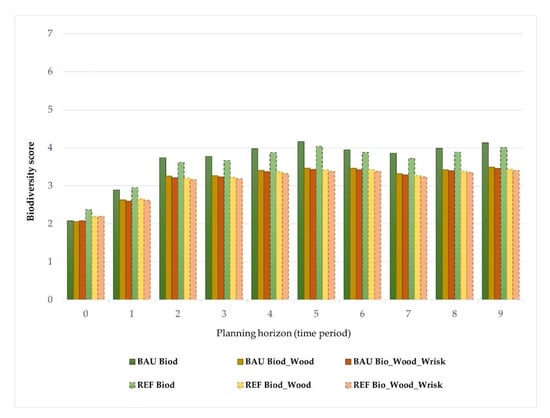
Figure 2.
Trends in the supply of biodiversity for the set of the optimal-solutions and local climate current (Business as usual (BAU), solid border) and changing (high climate forcing (REF), dashed border) conditions, for each 10-year period, over the 90-year planning horizon (from t0 = 2017 to t9 = 2106).
All the above-mentioned optimal solutions (Table 5) depict the relationship of different FMMs strategies for both climate change scenarios. The analysis of solution #2 which promotes and increases timber yield, intensified the distribution of cFMMs. While these results appear reasonable, is it notable that similar FMMs would probably be chosen without requesting any aspect of fuel treatment considerations across the 90-years of planning horizon. In contrast, the aFMMs accumulate a generous amount of biodiversity, due to their active promotion of native species, they create distinctly more species-rich and structurally diversified stands. The spatial distribution linking FMMs to biodiversity scores depicts the similarity between Fagaceae species pedunculate oak and cork oak.
When maximizing biodiversity without restrictions (Solution#1), a significant decrease in eucalypt plantations was observed (Figure 3). The transition from a predominantly eucalyptus forest to plantations of native species is evident. Indeed, after the first planning period, it is possible to convert eucalyptus stands essentially into maritime pine, followed by pedunculate and cork oak plantations. At the end of the planning horizon, the landscape was proposed to be occupied by maritime pine (54%), followed by cork oak (26%), pedunculate oak (18%) and less than 1% (41 ha) for chestnut, with no area ascribed to eucalypt plantations (Figure 3). Considering the combined effect of minimal timber production and fluctuation constraints (Solution# 2), the same area transference pattern was followed with respect to the aFMMs, towards a more similar distribution of species in the landscape, but in this case preserving up to 29% of the eucalyptus plantations and reassigned the remaining area to maritime pine (32%), oaks forest (33% total area), and to a less extent, chestnut (ca 4%). Last, to handle biodiversity with wood supply and wildfire risk constraints (Solution#3), the model responded by modifying more than a half of the landscape area to alternative forest species, and the corresponding area distribution showed a relatively homogeneous pattern with the previous solution#2.
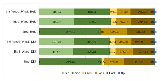
Figure 3.
Landscape optimal area distribution (total area covers 14,765 hectares) per species and local-climate scenarios at the end of the planning horizon (90-years). (Euc: Eucalyptus globulus; Pine: Pinus pinaster; Chest: Castanea sativa; Poak: Quercus robur; Coak: Quercus suber, Rp: riparian species).
On the other hand, chestnut areas increase with the reconversion of eucalyptus stands (Figure 3). Riparian species are included in all optimal solutions with minimum hectares (101.44 ha) to be allocated according to area constraints of the LP-model. The proposed landscape achieves the set of conservation, production, and protection goals through a mosaic of current (cFMM1–cFMM4) and alternative (aFMM5–aFMM8) forest management models. However, with adjustments to the current FMMs, such as cFMM1 and cFMM2, where it is intended to preserve maritime pine but remove eucalyptus. In addition, cFMM4 is completely removed from the optimal landscape distribution in solution#1. In general, the set of landscape optimal solutions has the largest area covered with aFMM5 (maritime pine) (Figure 3).
Undoubtedly, cFMMs 1, 2, and 4 with eucalyptus are not an option when the objective is to maximize biodiversity conservation values. There is a preference for longer rotations of maritime pine (aFMM5), cork oak (aFMM7), and pedunculated oak (aFMM6). Regarding the fuel management schedule the results of the first landscape solution also revealed that “no fuel treatment” periodicity is selected in more than 98% of the FMM prescriptions (Figure 4). Contrariwise, when we are optimizing biodiversity conservation by combining a limit of 9 million cubic meters for harvested wood, together with a maximum of 10% fluctuations between timber harvesting from consecutive planning periods (Solution#2), a set of different fuel treatment periodicities is selected with a preference for “no fuel treatment”, trailed by fuel treatments with a periodicity of 10 and 15-years in specific prescriptions of eucalyptus and pure maritime pine (Figure 4). In contrast when assessing the trade-off between biodiversity and the wildfire vulnerability of solution#3, a range biodiversity score between 2.59 and 3.46 coupled with more periodicity of one- and five-years of fuel treatments in eucalyptus prescription are chosen (Figure 4). There is evidence that the fuel reduction schedule can impact the contrast between FMMs in plantations forest and it is often coupled for optimization purposes. In this case, the fuel reduction option applied annually and every five years in parallel to the representation of species with higher productivity such as eucalyptus can provide a minimum average of wildfire resistance (WRISK > 3), without disregarding biodiversity conservation values and balanced levels of wood production over the 90-years.
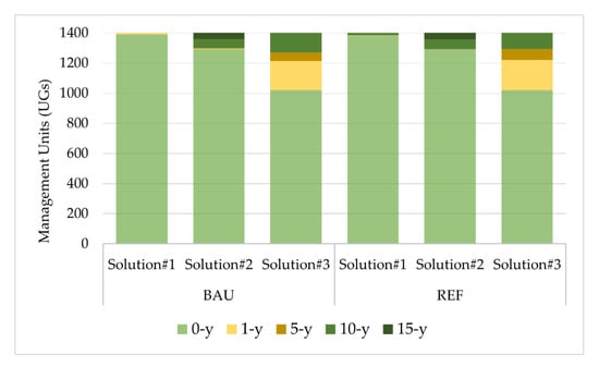
Figure 4.
Fuel treatment prescriptions (no fuel treatment: 0-y; annually: 1-y; each 5-years; 10-years; and each 15-years) optimal distribution across the landscape, for each optimal solution and local-climate scenarios.
The dynamic range of the forest landscape over time could be beneficial to biodiversity as it covers the stated key wood production goals (Table 6). Positive changes are observed in terms of biodiversity scores across the landscape when considering only maximize the provision of biodiversity levels. In addition, 5.3 million cubic meters were harvested (including thinning) in the optimal solution#1, reflecting the effect of no target constraints on wood production. Considering the harvested wood (9 × 10⁶ m3) inter-period fluctuations constraints, and wildfire mitigation measures (wildfire resistance > 3) in the VA_CSA, an average biodiversity score can be safely provided over the planning horizon. Due to more broadleaves across the landscape, there is an increase in sawmill and hardwoods, in parallel to the representation of species with higher productivity such as eucalyptus. Additionally, there are no significant differences in the distribution of wood production along each 10-year planning period when comparing both optimal solutions #2 and #3 (Table 6). The management alternatives included in the model proved to be sufficiently flexible to obtain the desired level of timber yield, both in standing volume and in the harvest distribution along the planning horizon, while ensuring acceptable levels of biodiversity score and reasonable wildfire resistance.
Table 6.
Timber provision, average volume harvested and volume of ending inventory for the three optimal-solutions, under current (BAU) and changing (REF) climate conditions.
Regarding the distribution of FMMs across the landscape in the relationship between biodiversity conservation and wood production, both BAU and REF solutions were similar in assessing the supply of forest ES (Table 5). According to optimal solution#1 for the REF scenario, under climate change conditions, biodiversity values slightly decrease from 0.5 to 0.3 over the planning horizon (Figure 2). Specifically, in the REF solution, rotation lengths were changed (either extended or shortened) for management units where Fagaceae species (i.e., pedunculate or cork oak) were not an option due to land aptitude limitations. For both climate scenarios, the volumes harvested and standing at the end of each planning decade were enhanced by the need for 9 million cubic meters, when compared to the optimal-solution#1. The harvested volumes ranged from a minimum of 0.57 (corresponding to the seventh period) while the maximum value reached 1.9 × 10⁶ m3 in the last decade of the planning horizon. The difference between the local scenarios from a biodiversity perspective is the higher values in climatic variables, compatible with RCP8.5 scenario, which correlate with the amount of shrubby understory through different intervals of surface fuel treatments (0, 1, 5, 10, and 15-years) and, consequently, shrub volume increases. This is in line with the general knowledge that the increase in biodiversity scores depends on a change in the understory status in terms of biomass (Mg. ha−1), which in turn changes with a rise in temperature and precipitation. On the other hand, competition for resources (i.e., light and water) reduces shrub growth over time [86].
The alternative management planning was designed to guarantee a desirable biodiversity score at the local level. Therefore, the landscape managed by our alternative approach (measured as tree composition and understory biomass accumulation) can potentially contribute to the conservation of biodiversity compared to the original scale of management unit assigned to current FMMs (Figure 1). Hence, the set of FMMs was distributed throughout the landscape, according to their performance in relation to the proposed management objectives (Table 1). The objectives can be achieved by integrating native species—alternative forest management models—further strengthening the heterogeneity of the natural habitat and structural diversity. At the forest species level, FMM5 and FMM7 clearly dominate the alternative landscape map-distribution, followed by FMM6 and some scattered occurrences of FMM3 (Figure 3).
4. Discussion
In this research, a landscape-level LP-RMC was extended to integrate a biodiversity-oriented forest management indicator and two local climate scenarios, i.e., business-as-usual (BAU) and REF (with a RCP 8.5) to measure the quantitative impact of forest management models on the potential biodiversity landscape provision. The proposed methodology explores the instrumental interaction between forest management models and biodiversity levels at the stand and landscape scales in the face of climate change, using tree species composition and understory vegetation as biodiversity proxies. Likewise, the application of a simulation-optimization framework to guide forest actors in considering optimal practices to safeguard future biodiversity; seeking to benefit native forest species, while other conservation commitments are reached in long-term forest management. For that purpose, several forest management models (four current and four alternative FMMs), through different periodicity of fuel treatments and effects of local-climate change on biodiversity indicators and related proxies were tested.
In the last thirty years, the integration of biodiversity into forest management has been classified and evaluated in accordance with different attributes such as model components, forest management elements, or biodiversity indicators. However, landscapes are rarely managed to provide levels of biodiversity, in part because the indicators remain complex, and new key-related variables need to be considered to drive management decisions [14,92]. Given the long rotations used in several forest systems, it is essential to have a set of indicators that encompass such long-term time scales and which values can be assessed periodically, after a particular management intervention, but also at the end of the planning horizon. In that sense, the biodiversity indicator used in the present study aims to fulfil such purpose, as it is a function of species composition (e.g., chestnut, cork oak, eucalypt, pine, pure pedunculate oak, and riparian trees), the stand age, and understory biomass accumulation, and there is a linear trade-off between area of each FMM and the biodiversity indicator. Several researchers identified that the understory vegetation is a practical indicator and a major driver of many forest processes such as forest productivity, litter decomposition and light interception [47,50,93]. In fact, our research CSA area provides relevant outputs addressing the understory shrub conditions, thus allowing differentiation between forest characterization/attributes of higher or lower importance of biodiversity. The newly criteria used to classify the biodiversity proxies in Vale de Sousa have proved to be a practical indicator for assessing forest biodiversity provisions under forest management plans in Europe [94]. It is important to remark that 21 studies reviewed by Thompson et al. [95] reported that in 76% of the cases, vertebrate and arthropod diversity are positively correlated with plant diversity (measured as tree species and understory richness), establishing a direct relationship between increased biodiversity and forest productivity. Further, forest stand structural variables derived from inventories can help enhance management plans to place European forests on the path to an uncertain future [94].
As far as we are concerned, indicators such as the structural heterogeneity of both tree species and understory may reflect better the biodiversity value than the amount of deadwood or the number of large trees [96]. In Portugal, the richness and diversity of tree species are poor because most are single or two species stands. Even conservation valued cork oak woodlands are frequently mono—(cork oak only) or dual-specific (e.g., cork and holm oak) [46]. whilst in central Europe or Northern forested landscapes, we are dealing with a few different tree species, here biodiversity provision is not in the diversity of tree species but on the shrubby understory. Thus, shrub species composition considered in forest management planning is particularly important in Portugal since Mediterranean basin is one of the "hot spots" of biodiversity worldwide [97]. In this regard, increasing the availability of specific forest structures (e.g., dead wood and large trees) are not a strategy for achieving biodiversity goal across Portugal. Indeed, what make Portugal ecosystems interesting for biodiversity conservation is the mixture of shrub and grassland species underneath tree cover. Consequently, the relevance of pine, eucalypt, chestnut, and oak stands for conservation in these forested areas relies on the diversity and amount of shrub cover as an important habitat type for wildlife. This may impact the assessment of trade-offs between biodiversity and other ES. Nevertheless, these differences in outcome highlight the potential of this approach to be actively applied within CSAs to dictate the future biodiversity of forest production areas. Such an assumption, however, needs to be assessed in the future with increased wildfire hazard in shrub encroached stands, which may ultimately lead to loss of conservation value.
Our results are placed in the context of forest management and practically revealed no significant reductions in outcomes of biodiversity indicators with the rise in wood production. Further, we aimed to sustain the supply of timber at levels suitable for each climate scenario. Thereby, well-balanced results arose when diversity was actively promoted with new FMMs as part of a sustainable management concept. Liang et al. [13] stated that there is a predominant positive biodiversity-productivity relationship in global forests. Regarding this component, our results suggested that there was not significant trade-off between biodiversity and sustainable wood production. These results agree with a study for then forest landscapes across Europe [96] were they stated that almost no reduction in biodiversity indicators are associated with an increase in sustainable wood production. Indeed, in the recent years, potential synergies have been discussed in the connection between a landscape biodiversity conservation and wood production [21,46,98,99].
The cFMMs have typical characteristics associated with lower biodiversity scores than the aFMMs in the same period. In fact, the cFMMs 1, 2, and 4 with eucalypt species had a reduced biodiversity score over the entire 90-year horizon. This is also in agreement with the finding in the work by Proença et al. [100] and Goded et al. [101] from Spain, where biodiversity in eucalyptus stands is compared to native stands, and the results showed the lowest values was precisely for eucalyptus. Indeed, diversity and composition of understory vegetation tended to be higher in native forests and shrublands, and lowest in eucalypt plantations in several stages (young, intermediate and mature) [102]. Eucalyptus plantations display extremely low biological and aesthetic diversity; although, they seem to be admirably adapted to VA_CSA conditions. It is well associate with climax species and allow the development of diverse shrub layer. The presence of eucalypt may be instrumental to landscape heterogeneity and generate financial resources to support set-aside conservation areas, thus contributing to landscape-level biodiversity. Basically, the management activities of the cFMMs landscape-solution for our CSA, results in less biodiversity score due to essentially two factors: shorter rotations from the introduced eucalyptus species resulting in a younger forests and more compressed age class structure, and more coniferous trees over lager areas. Nevertheless, the combined effect of market, technical and human capacities play a major role in keeping the current almost total dominance of the production of the eucalyptus and maritime pine systems [88]. Still, due to the recent changes on the National Forest Policy, there are now stronger planting restrictions on eucalyptus, and thus the forest owners are looking for native alternative species for timber production, resin and cork production, and wildfire risk reduction.
Alternative FMMs are encouraged, especially in addressing climate change and potential future conditions in forest productivity. The optimal-solutions depict the dominance of native species in the new FMMs for our case study area. Eucalyptus stands exchanges by maritime pine and oak forests areas contributed to the biodiversity increase along the planning horizon. Maritime pine stands plantations (aFMM5) retain a significant recreation interest, as they are widely used for summer picnics. In the past, pedunculated oaks dominated the landscapes in the northern Portugal. aFMM6 and aFMM7 relates to native species of Fagaceae where, from a biodiversity perspective, there is a larger proportion of broadleaves. aFMM3 has a reasonable biodiversity score values, by the richness associated vegetation of Castanea sativa species. Although this species is associated to high values of biodiversity, the chosen prescriptions have shorter years of rotation than the Q. robur and Q. suber species (aFMM6 and aFMM7, respectively). aFMM8 (riparian system) have the highest biodiversity score values over the 90-years of planning period. aFMM8 will contribute to biodiversity by providing habitats for specific flora and fauna, both in the tree itself and in the flooded root system.
In this respect, the aFMMs demonstrate higher values than de cFMMs in terms of species richness, shrubby understory diversity, and stand structure. This is also associated with the periodicity of fuel treatments on the selected prescriptions of aFMM and cFMM and the corresponding impact on the accumulation of fuel understory. The set of aFMM fits properly with the general goal to manage forests for increased resistance and resilience. Horl et al. [103] reviewed the performance of adaptive forest management strategies and identified changes in species composition as one of the most resilience-oriented strategies recommended among adaptation scenarios in relation to multiple goods and services, including wood production and biodiversity. In fact, it is a major concept for facing an uncertain future in forestry [104].
The local-climate scenarios applied did not cause necessarily different outputs at the case study level. The classification of biodiversity scores suggests that the increase of temperature and precipitation from the reference local-climate scenario, compared with the BAU scenario, has a limited impact on the provision of the overall biodiversity. While the frame scenarios did not make a big difference, the outcomes of the silvicultural treatment showed interesting patterns. Previous research in Vale de Sousa with a focus on simultaneous maximization of multiple objectives has shown that biodiversity conservation values are lower (average values 1.52) when only current FMMs are assigned to all suitable management units, mainly explained by the proportion of eucalyptus [62,98]. Our optimal forest management solution accomplishes an increase of 2.52 for maximizing biodiversity concerns with the share of native species as alternative FMMs across the current landscape (Biodiversity score = 3.82), and a slight increase of 1.78 and 1.72, when it reaches forest actor interests in wood provisioning and wildfires reduction, respectively.
Some limitations might be underlined. For example, the understory biodiversity relates mostly with shrub biomass, assuming that shrub cover is essential for wildlife, but do not reflect plant diversity. This can be improved in future assessments. There is also the degree of uncertainty that is linked to the results—mainly due to the use of empirical growth and yield models, disregarding the inclusion of physiological data, but also due to the derived assumptions of expected climate change effects on forest growth under the REF scenario. Although our database did not allow to simulate the effects of large tree removal on wood production and biodiversity it is know that large trees are frequently used for bird nesting namely threatened bird raptors such as the red kite (Milvus milvus) which in Iberian Peninsula may nest is pine plantations similar to those in our study area [105].
The strong relationship between the ecological and economic functions of forest services, under the impact of environmental factors, is crucial for the stakeholders decision-making processes. In this regard, future work directions screen a focus on the economic representation of ES values (e.g., net present value and soil expectation value) to allow a complete interpretation and efficient use of the described LP-RCM.
5. Conclusions
One of the major challenges today is how to balance the increasing demand for species diversification whilst targeting increased supply of other ES to ensure profitability for forest owners? Current management in Vale do Sousa is often inefficient and undersupplies forest biodiversity. The present research highlighted the concern with the provision of biodiversity ecosystem and prompted to the development of an approach to improve the biodiversity conservation outcomes through each FMMs. In the present research, desirable biodiversity can be delivered with levels of sustainable wood production and reduced socio-ecological risk.
Our landscape-level RCM together with a LP-based optimization method is used to reconcile biodiversity conservation in Vale de Sousa with both forest actors targets in timber production and resistance to wildfire, while contributing to mitigate climate change. Remarkably, most of the recommended LP-RCM solutions were robust enough to support the simultaneous provision of a minimum standard of outcome for timber values and wildfire resistance through diversification in the forest species composition, with an increase in age rotation at a landscape-level. The results noticed an interesting comparison between cFMMs and aFMMs associated with the selected prescriptions and the corresponding impact on the accumulation of fuel load. Considering the distinctiveness of native forests, eucalyptus plantations cannot replace native species to enhance conservation outcomes. For the combining tree species and understory indicator, we created the score that gives value to each forest species/FMMs according to its richness and its contribution to biodiversity. The former has fostered the ability to provide forest managers with a ranking of FMM according to the biodiversity score. The biodiversity management-oriented indicator is appropriate for use by several forest-sector actors. The results can be useful in conservation planning to estimate how soon a certain level of biodiversity can be reached. In addition to implementing aFMMs in practice appears to be a real chance for new forest management principles, to make inroads in the national policy processes planning, forest certification schemes, or market payments for ecosystem services. In this sense, we see our newly developed biodiversity criteria integrated into a LP-RCM as highly promising for the integration and interpretation of biodiversity proxies into adaptive forest management planning and provide a promising avenue to help address the provision of ecosystem services.
Author Contributions
All authors made a significant contribution to the present manuscript preparation. B.B. was involved in conceptualization, data collection and computation, biodiversity indicator methodology and implementation, results analysis and interpretation, and wrote the paper; M.N.B. was involved in the biodiversity indicator methodology, manuscript reviewing and editing; A.R.R. assisted in model methodology development and implementation, manuscript reviewing and editing; M.M. assisted in biodiversity indicator computation and RCM development and implementation; S.M. was involved in data collection and computation and LP-model methodology development; J.G.B. was involved as research coordinator, project manager and in conceptualization, development of methodologies and manuscript writing and final reviewing. All authors have read and agreed to the published version of the manuscript.
Funding
The first author’s research activities were funded by BIOECOSYS project, “Forest ecosystem management decision-making methods: an integrated bioeconomic approach to sustainability”, grant number LISBOA-01-0145-FEDER-030391, PTDC/ASP-SIL/30391/2017. This research was also funded by MODFIRE project “A multiple criteria approach to integrate wildfire behaviour in forest management planning with the reference” (PCIF/MOS/0217/2017); NOBEL project “Novel business models to sustainably supply forest ecosystem services”, under the umbrella of ERA-NET cofund ForestValue (Horizon 2020 research and innovation programme grant agreement Nº773324), and CERTFOR project “Effects of forest certification on the conservation of cork oak woodlands” PTDC/ASP-SIL/31253/2017.
Acknowledgments
Authors would like to thank Associação Florestal do Vale do Sousa for assistance with study area characterization and forest inventory fieldwork. The authors also thank the Forest Research Centre, a research unit funded by Fundação para a Ciência e a Tecnologia I.P. (FCT), Portugal within UID/AGR/00239/2019 and UIDB/00239/2020 for their support and Centre for Applied Ecology “Prof. Baeta Neves” (CEABN-InBIO) research unit funded FEDER funds through the Operational Programme for Competitiveness Factors—COMPETE and by National Funds through FCT under the UID/BIA/50027/2013 and POCI-01-0145-FEDER-006821. M.N. Bugalho was funded by contract DL 57/2016/CP1382/CT0030. Research activities of Susete Marques were supported by the national funds through FCT, in the scope of Norma Transitória–DL57/2016/CP1382/CT15.
Conflicts of Interest
The authors declare no conflict of interest.
Appendix A
The approach presented in Section 2.4. Biodiversity management-oriented indicators, is based on several forest management models (FMMs), assuming a biodiversity score that increases with shrub cover and changes according to tree composition and forest structure. Their estimation proceeds as follows:
Appendix A.1. Tree Species Composition
Tree species proportion and age—The contribution of each species to biodiversity proxies is also scored according to the corresponding age assigning higher values to higher ages. The biodiversity goals should then enable differentiation between tree species of higher or lower importance for biodiversity as represented below:
Table A1.
Species proportion, description, minimum and maximum values used to define the FMM1 biodiversity score.
Table A1.
Species proportion, description, minimum and maximum values used to define the FMM1 biodiversity score.
| #1. Species Proportion | Description | Scores |
|---|---|---|
| FMM1—Maritime pine dominant | Differentiation between tree species of higher or lower importance for biodiversity. | The mixed stands of maritime pine and eucalypts biodiversity range from 1 to 3 according to the dominance of eucalypt and pine, respectively |
Maximum score Pb = 3 and Maximum Score Ec = 2; Maximum rotation Pb = 50 years. Minimum score Pb = 2 and Minimum Score Ec = 1; Maximum rotation Ec = 12 years.
Table A2.
Species proportion, description, minimum and maximum values used to define the FMM2 biodiversity score.
Table A2.
Species proportion, description, minimum and maximum values used to define the FMM2 biodiversity score.
| #1. Species Proportion | Description | Scores |
|---|---|---|
| FMM2—Eucalypt dominant | Differentiation between tree species of higher or lower importance for biodiversity. | The mixed stands of maritime pine and eucalypts biodiversity range from 1 to 3 according to the dominance of eucalypt and pine, respectively. |
Maximum Score Ec = 2 and Maximum score Pb = 3; Maximum rotation Pb = 50 years. Minimum score Ec= 1 and Minimum Score Pb = 2; Maximum rotation Ec = 12 years.
Table A3.
Species proportion, description, minimum and maximum values used to define the FMM3 biodiversity score.
Table A3.
Species proportion, description, minimum and maximum values used to define the FMM3 biodiversity score.
| #1. Species Proportion | Description | Scores |
|---|---|---|
| FMM3—Chestnut | Differentiation between tree species of higher or lower importance for biodiversity. | Chestnut is associated to a biodiversity maximum partial score = 4 |
Maximum score Ct = 4, Minimum score Ct = 3; Maximum rotation = 55.
Table A4.
Species proportion, description, minimum and maximum values used to define the FMM4 biodiversity score.
Table A4.
Species proportion, description, minimum and maximum values used to define the FMM4 biodiversity score.
| #1. Species Proportion | Description | Scores |
|---|---|---|
| FMM4—Eucalypt | Differentiation between tree species of higher or lower importance for biodiversity. | Eucalypt pure stands are associated to a maximum partial score = 2 |
Maximum score Ec = 2, Minimum score Ec = 1; Maximum rotation = 12.
Table A5.
Species proportion, description, minimum and maximum values used to define the FMM5 biodiversity score.
Table A5.
Species proportion, description, minimum and maximum values used to define the FMM5 biodiversity score.
| #1. Species Proportion | Description | Scores |
|---|---|---|
| FMM5—Pure maritime pine | Differentiation between tree species of higher or lower importance for biodiversity. | Maritime pure stands are associated to a maximum partial score = 3 |
Maximum score Pb = 3, Minimum score Pb =2; Maximum rotation = 50.
Table A6.
Species proportion, description, minimum and maximum values used to define the FMM6 biodiversity score.
Table A6.
Species proportion, description, minimum and maximum values used to define the FMM6 biodiversity score.
| #1. Species Proportion | Description | Scores |
|---|---|---|
| FMM6—Pedunculate oak | Differentiation between tree species of higher or lower importance for biodiversity. | Pedunculate oak stands are associated to a maximum partial score = 5 |
Maximum score Qr = 5, Minimum score Qr = 4; Maximum rotation = 60.
Table A7.
Species proportion, description, minimum and maximum values used to define the FMM7 biodiversity score.
Table A7.
Species proportion, description, minimum and maximum values used to define the FMM7 biodiversity score.
| #1. Species Proportion | Description | Scores |
|---|---|---|
| FMM7—Cork oak | Differentiation between tree species of higher or lower importance for biodiversity. | Cork oak stands are associated to a maximum partial score = 5 |
Maximum score Sb = 5, Minimum score Sb = 4; Maximum rotation = 90.
Table A8.
Species proportion, description, minimum and maximum values used to define the FMM8 biodiversity score.
Table A8.
Species proportion, description, minimum and maximum values used to define the FMM8 biodiversity score.
| #1. Species Proportion | Description | Scores |
|---|---|---|
| FMM8—Riparian Systems | Differentiation between tree species of higher or lower importance for biodiversity. | Riparian stands are associated to a maximum partial score = 6 |
Maximum score Rp = 6, Minimum score Rp = 5; Maximum rotation = 90.
Appendix A.2. Understory Vegetation
Shrub biomass accumulation—An additional specific indicator based on shrub biomass quantification as per Botequim et al. [86] has been included. The corresponding “biomass” indicator is measured using the corresponding biomass (Mg. ha−1) under canopy cover associated with habitat- biodiversity benefits, and classified as follows:
Table A9.
Shrub cover, description, minimum and maximum values used to define the biomass biodiversity score.
Table A9.
Shrub cover, description, minimum and maximum values used to define the biomass biodiversity score.
| #2. Shrub Cover | Description | Scores |
|---|---|---|
| FMM1—Maritime pine dominant FMM2—Eucalypt dominant FMM3—Chestnut FMM4—Pure Eucalypt FMM5—Pure maritime pine FMM6—Pedunculate oak FMM7—Cork oak FMM8—Riparian system | The corresponding “biomass” indicator was measured by Botequim et al., 2015 | The shrub cover of FMMs 1 to 7 ranges between “0” and “1” |
x = 3, 4, 5, 6, 7 e 8
Appendix A.3. Total Biodiversity Score (Example)
The total biodiversity scores for the Vale de Sousa CSA is computed by the partial biodiversity score—tree species composition (Appendix A.1.) and the partial score—shrub cover (Appendix A.2.)
References
- Cardinale, B.J.; Duffy, J.E.; Gonzalez, A.; Hooper, D.U.; Perrings, C.; Venail, P.; Narwani, A.; Mace, G.M.; Tilman, D.; Wardle, D.A.; et al. Biodiversity Loss and Its Impact on Humanity. Nature 2012, 486, 59–67. [Google Scholar] [CrossRef]
- Pretzsch, H.; Knoke, T. Forest management planning in mixed-species forests. In Mixed-Species Forests. Ecology and Management; Pretzsch, H., Forrester, D.I., Bauhus, J., Eds.; Springer: Berlin/Heidelberg, Germany, 2017; pp. 503–544. ISBN 978-3-662-54553-9. [Google Scholar]
- Parrot, L.; Kange, H. An introduction to complexity science. In Managing Forests as Complexity Adaptatiove Systems; Messier, C., Puettmann, K.J., Coates, D., Eds.; Routledge: Abingdon, UK, 2014; pp. 17–32. ISBN 978-1-138-77969-3. [Google Scholar]
- Eyvindson, K.; Repo, A.; Mönkkönen, M. Mitigating Forest Biodiversity and Ecosystem Service Losses in the Era of Bio-Based Economy. For. Policy Econ. 2018, 92, 119–127. [Google Scholar] [CrossRef]
- Lindenmayer, D.B.; Margules, C.R.; Botkin, D.B. Indicators of Biodiversity for Ecologically Sustainable Forest Management. Conserv. Biol. 2000, 14, 941–950. [Google Scholar] [CrossRef]
- Balvanera, P.; Pfisterer, A.B.; Buchmann, N.; He, J.-S.; Nakashizuka, T.; Raffaelli, D.; Schmid, B. Quantifying the Evidence for Biodiversity Effects on Ecosystem Functioning and Services: Biodiversity and Ecosystem Functioning/Services. Ecol. Lett. 2006, 9, 1146–1156. [Google Scholar] [CrossRef]
- Díaz, S.; Fargione, J.; Chapin, F.S.; Tilman, D. Biodiversity Loss Threatens Human Well-Being. PLoS Biol. 2006, 4, e277. [Google Scholar] [CrossRef]
- Paquette, A.; Messier, C. The Effect of Biodiversity on Tree Productivity: From Temperate to Boreal Forests: The Effect of Biodiversity on the Productivity. Global Ecol. Biogeogr. 2011, 20, 170–180. [Google Scholar] [CrossRef]
- Tilman, D.; Reich, P.B.; Isbell, F. Biodiversity Impacts Ecosystem Productivity as Much as Resources, Disturbance, or Herbivory. Proc. Natl. Acad. Sci. USA 2012, 109, 10394–10397. [Google Scholar] [CrossRef]
- Isbell, F.; Craven, D.; Connolly, J.; Loreau, M.; Schmid, B.; Beierkuhnlein, C.; Bezemer, T.M.; Bonin, C.; Bruelheide, H.; de Luca, E.; et al. Biodiversity Increases the Resistance of Ecosystem Productivity to Climate Extremes. Nature 2015, 526, 574–577. [Google Scholar] [CrossRef]
- Lefcheck, J.S.; Byrnes, J.E.K.; Isbell, F.; Gamfeldt, L.; Griffin, J.N.; Eisenhauer, N.; Hensel, M.J.S.; Hector, A.; Cardinale, B.J.; Duffy, J.E. Biodiversity Enhances Ecosystem Multifunctionality across Trophic Levels and Habitats. Nat. Commun. 2015, 6. [Google Scholar] [CrossRef]
- Gamfeldt, L.; Snäll, T.; Bagchi, R.; Jonsson, M.; Gustafsson, L.; Kjellander, P.; Ruiz-Jaen, M.C.; Fröberg, M.; Stendahl, J.; Philipson, C.D.; et al. Higher Levels of Multiple Ecosystem Services Are Found in Forests with More Tree Species. Nat. Commun. 2013, 4. [Google Scholar] [CrossRef]
- Liang, J.; Crowther, T.W.; Picard, N.; Wiser, S.; Zhou, M.; Alberti, G.; Schulze, E.-D.; McGuire, A.D.; Bozzato, F.; Pretzsch, H.; et al. Positive Biodiversity-Productivity Relationship Predominant in Global Forests. Science 2016, 354, aaf8957. [Google Scholar] [CrossRef] [PubMed]
- Ratcliffe, S.; Wirth, C.; Jucker, T.; van der Plas, F.; Scherer-Lorenzen, M.; Verheyen, K.; Allan, E.; Benavides, R.; Bruelheide, H.; Ohse, B.; et al. Biodiversity and Ecosystem Functioning Relations in European Forests Depend on Environmental Context. Ecol. Lett. 2017, 20, 1414–1426. [Google Scholar] [CrossRef] [PubMed]
- Butchart, S.H.M.; Walpole, M.; Collen, B.; van Strien, A.; Scharlemann, J.P.W.; Almond, R.E.A.; Baillie, J.E.M.; Bomhard, B.; Brown, C.; Bruno, J.; et al. Global Biodiversity: Indicators of Recent Declines. Science 2010, 328, 1164–1168. [Google Scholar] [CrossRef]
- Lindner, M.; Fitzgerald, J.B.; Zimmermann, N.E.; Reyer, C.; Delzon, S.; van der Maaten, E.; Schelhaas, M.-J.; Lasch, P.; Eggers, J.; van der Maaten-Theunissen, M.; et al. Climate Change and European Forests: What Do We Know, What Are the Uncertainties, and What Are the Implications for Forest Management? J. Environ. Manag. 2014, 146, 69–83. [Google Scholar] [CrossRef] [PubMed]
- Seidl, R.; Thom, D.; Kautz, M.; Martin-Benito, D.; Peltoniemi, M.; Vacchiano, G.; Wild, J.; Ascoli, D.; Petr, M.; Honkaniemi, J.; et al. Forest Disturbances under Climate Change. Nat. Clim. Chang. 2017, 7, 395–402. [Google Scholar] [CrossRef]
- Baskent, E.Z. Exploring the Effects of Climate Change Mitigation Scenarios on Timber, Water, Biodiversity and Carbon Values: A Case Study in Pozantı Planning Unit, Turkey. J. Environ. Manag. 2019, 238, 420–433. [Google Scholar] [CrossRef]
- Lindner, M.; Maroschek, M.; Netherer, S.; Kremer, A.; Barbati, A.; Garcia-Gonzalo, J.; Seidl, R.; Delzon, S.; Corona, P.; Kolström, M.; et al. Climate Change Impacts, Adaptive Capacity, and Vulnerability of European Forest Ecosystems. For. Ecol. Manag. 2010, 259, 698–709. [Google Scholar] [CrossRef]
- Ezquerro, M.; Pardos, M.; Diaz-Balteiro, L. Integrating Variable Retention Systems into Strategic Forest Management to Deal with Conservation Biodiversity Objectives. For. Ecol. Manag. 2019, 433, 585–593. [Google Scholar] [CrossRef]
- Felton, A.; Lindbladh, M.; Brunet, J.; Fritz, Ö. Replacing Coniferous Monocultures with Mixed-Species Production Stands: An Assessment of the Potential Benefits for Forest Biodiversity in Northern Europe. For. Ecol. Manag. 2010, 260, 939–947. [Google Scholar] [CrossRef]
- Keenan, R.J. Climate Change Impacts and Adaptation in Forest Management: A Review. Ann. For. Sci. 2015, 72, 145–167. [Google Scholar] [CrossRef]
- Brunette, M.; Foncel, J.; Kéré, E.N. Attitude towards Risk and Production Decision: An Empirical Analysis on French Private Forest Owners. Environ. Modeling Assess. 2017, 22, 563–576. [Google Scholar] [CrossRef]
- Seibold, S.; Gossner, M.M.; Simons, N.K.; Blüthgen, N.; Müller, J.; Ambarlı, D.; Ammer, C.; Bauhus, J.; Fischer, M.; Habel, J.C.; et al. Arthropod Decline in Grasslands and Forests Is Associated with Landscape-Level Drivers. Nature 2019, 574, 671–674. [Google Scholar] [CrossRef]
- Baker, S.C.; Spies, T.A.; Wardlaw, T.J.; Balmer, J.; Franklin, J.F.; Jordan, G.J. The Harvested Side of Edges: Effect of Retained Forests on the Re-Establishment of Biodiversity in Adjacent Harvested Areas. For. Ecol. Manag. 2013, 302, 107–121. [Google Scholar] [CrossRef]
- Fedrowitz, K.; Koricheva, J.; Baker, S.C.; Lindenmayer, D.B.; Palik, B.; Rosenvald, R.; Beese, W.; Franklin, J.F.; Kouki, J.; Macdonald, E.; et al. Can Retention Forestry Help Conserve Biodiversity? A Meta-analysis. J. Appl. Ecol. 2014, 51, 1669–1679. [Google Scholar] [CrossRef]
- Gustafsson, L.; Kouki, J.; Sverdrup-Thygeson, A. Tree Retention as a Conservation Measure in Clear-Cut Forests of Northern Europe: A Review of Ecological Consequences. Scand. J. For. Res. 2010, 25, 295–308. [Google Scholar] [CrossRef]
- Rosenvald, R.; Lõhmus, A. For What, When, and Where Is Green-Tree Retention Better than Clear-Cutting? A Review of the Biodiversity Aspects. For. Ecol. Manag. 2008, 255, 1–15. [Google Scholar] [CrossRef]
- Bauhus, J.; Puettmann, K.; Messier, C. Silviculture for Old-Growth Attributes. For. Ecol. Manag. 2009, 258, 525–537. [Google Scholar] [CrossRef]
- Gustafsson, L.; Baker, S.C.; Bauhus, J.; Beese, W.J.; Brodie, A.; Kouki, J.; Lindenmayer, D.B.; Lõhmus, A.; Pastur, G.M.; Messier, C.; et al. Retention Forestry to Maintain Multifunctional Forests: A World Perspective. BioScience 2012, 62, 633–645. [Google Scholar] [CrossRef]
- O’Hara, K.L. Multiaged Silviculture: Managing for Complex Forest Stand Structures; Oxford University Press: New York, NY, USA, 2014; ISBN 978-0-19-870306-8. [Google Scholar]
- Franklin, J.F.; Berg, D.F.; Thornburg, D.; Tappeiner, J.C. Alternative silvicultural approaches to timber harvesting: Variable retention harvest systems. In Creating a Forestry for the 21st Century: The Science of Ecosystem Management; Kohm, K.A., Franklin, J.F., Eds.; Island Press: Washington, WA, USA, 1997; pp. 111–139. [Google Scholar]
- Shea, E.L.; Schulte, L.A.; Palik, B.J. Decade-Long Bird Community Response to the Spatial Pattern of Variable Retention Harvesting in Red Pine (Pinus Resinosa) Forests. For. Ecol. Manag. 2017, 402, 272–284. [Google Scholar] [CrossRef]
- Kouki, J.; Löfman, S.; Martikainen, P.; Rouvinen, S.; Uotila, A. Forest Fragmentation in Fennoscandia: Linking Habitat Requirements of Wood-Associated Threatened Species to Landscape and Habitat Changes. Scand. J. For. Res. 2001, 16, 27–37. [Google Scholar] [CrossRef]
- Mori, A.S.; Tatsumi, S.; Gustafsson, L. Landscape Properties Affect Biodiversity Response to Retention Approaches in Forestry. J. Appl. Ecol. 2017, 54, 1627–1637. [Google Scholar] [CrossRef]
- Augustynczik, A.L.D.; Asbeck, T.; Basile, M.; Bauhus, J.; Storch, I.; Mikusiński, G.; Yousefpour, R.; Hanewinkel, M. Diversification of Forest Management Regimes Secures Tree Microhabitats and Bird Abundance under Climate Change. Sci. Total Environ. 2019, 650, 2717–2730. [Google Scholar] [CrossRef] [PubMed]
- Coşofreţ, C.; Bouriaud, L. Which Silvicultural Measures Are Recommended To Adapt Forests To Climate Change? A Literature Review. Bull. Transilv. Brasov. For. Wood Ind. Agric. Food Eng. 2019, 12, 13–34. [Google Scholar]
- Augustynczik, A.L.D.; Yousefpour, R. Balancing Forest Profitability and Deadwood Maintenance in European Commercial Forests: A Robust Optimization Approach. Eur. J. For. Res. 2019, 138, 53–64. [Google Scholar] [CrossRef]
- Coote, L.; Dietzsch, A.C.; Wilson, M.W.; Graham, C.T.; Fuller, L.; Walsh, A.T.; Irwin, S.; Kelly, D.L.; Mitchell, F.J.G.; Kelly, T.C.; et al. Testing Indicators of Biodiversity for Plantation Forests. Ecol. Indic. 2013, 32, 107–115. [Google Scholar] [CrossRef]
- Franklin, J.F. Toward a New Forestry. American Forests. November/December 1989. pp. 37–44. Available online: https://andrewsforest.oregonstate.edu/publications/1059 (accessed on 8 January 2021).
- Gustafsson, L.; Bauhus, J.; Asbeck, T.; Augustynczik, A.L.D.; Basile, M.; Frey, J.; Gutzat, F.; Hanewinkel, M.; Helbach, J.; Jonker, M.; et al. Retention as an Integrated Biodiversity Conservation Approach for Continuous-Cover Forestry in Europe. Ambio 2020, 49, 85–97. [Google Scholar] [CrossRef]
- Hodge, S.J.; Peterken, G.F. Deadwood in British Forests: Priorities and a Strategy. Forestry 1998, 71, 99–112. [Google Scholar] [CrossRef]
- Karahalil, U.; Başkent, E.Z.; Sivrikaya, F.; Kılıç, B. Analyzing Deadwood Volume of Calabrian Pine (Pinus Brutia Ten.) in Relation to Stand and Site Parameters: A Case Study in Köprülü Canyon National Park. Environ. Monit. Assess. 2017, 189. [Google Scholar] [CrossRef]
- Smith, G.F.; Gittings, T.; Wilson, M.; French, L.; Oxbrough, A.; O’Donoghue, S.; O’Halloran, J.; Kelly, D.L.; Mitchell, F.J.G.; Kelly, T.; et al. Identifying Practical Indicators of Biodiversity for Stand-Level Management of Plantation Forests. Biodivers. Conserv. 2008, 17, 991–1015. [Google Scholar] [CrossRef]
- Arsenault, A.; Bradfield, G.E. Structural—Compositional Variation in Three Age-Classes of Temperate Rainforests in Southern Coastal British Columbia. Can. J. Botany 1995, 73, 54–64. [Google Scholar] [CrossRef]
- Bugalho, M.N.; Dias, F.S.; Briñas, B.; Cerdeira, J.O. Using the High Conservation Value Forest Concept and Pareto Optimization to Identify Areas Maximizing Biodiversity and Ecosystem Services in Cork Oak Landscapes. Agrofor. Syst. 2016, 90, 35–44. [Google Scholar] [CrossRef]
- Dearden, F.; Wardle, D. The Potential for Forest Canopy Litterfall Interception by a Dense Fern Understorey, and the Consequences for Litter Decomposition. Oikos 2008, 117, 83–92. [Google Scholar] [CrossRef]
- Ferris, R.; Peace, A.J.; Newton, A.C. Macrofungal Communities of Lowland Scots Pine (Pinus Sylvestris L.) and Norway Spruce (Picea Abies (L.) Karsten.) Plantations in England: Relationships with Site Factors and Stand Structure. For. Ecol. Manag. 2000, 131, 255–267. [Google Scholar] [CrossRef]
- Gao, T.; Hedblom, M.; Emilsson, T.; Nielsen, A.B. The Role of Forest Stand Structure as Biodiversity Indicator. For. Ecol. Manag. 2014, 330, 82–93. [Google Scholar] [CrossRef]
- Gendron, F.; Messier, C.; Comeau, P.G. Comparison of Various Methods for Estimating the Mean Growing Season Percent Photosynthetic Photon Flux Density in Forests. Agric. For. Meteorol. 1998, 92, 55–70. [Google Scholar] [CrossRef]
- Khanina, L.; Bobrovsky, M.; Komarov, A.; Mikhajlov, A. Modeling Dynamics of Forest Ground Vegetation Diversity under Different Forest Management Regimes. For. Ecol. Manag. 2007, 248, 80–94. [Google Scholar] [CrossRef]
- Paffetti, D.; Travaglini, D.; Buonamici, A.; Nocentini, S.; Vendramin, G.G.; Giannini, R.; Vettori, C. The Influence of Forest Management on Beech (Fagus Sylvatica L.) Stand Structure and Genetic Diversity. For. Ecol. Manag. 2012, 284, 34–44. [Google Scholar] [CrossRef]
- López, G.; Moro, M.J. Birds of Aleppo Pine Plantations in South-East Spain in Relation to Vegetation Composition and Structure. J. Appl. Ecol. 1997, 1257–1272. [Google Scholar] [CrossRef]
- Brockerhoff, E.G.; Jactel, H.; Parrotta, J.A.; Quine, C.P.; Sayer, J. Plantation Forests and Biodiversity: Oxymoron or Opportunity? Biodivers. Conserv. 2008, 17, 925–951. [Google Scholar] [CrossRef]
- Thompson, E.F.; Halterman, B.G.; Lyon, T.J.; Miller, R.L. Integrating Timber and Wildlife Management Planning. For. Chron. 1973, 49, 247–250. [Google Scholar] [CrossRef]
- Hof, J.G.; Joyce, L.A. A Mixed Integer Linear Programming Approach for Spatially Optimizing Wildlife and Timber in Managed Forest Ecosystems. For. Sci. 1993, 39, 816–834. [Google Scholar] [CrossRef]
- Hof, J.; Bevers, M.; Joyce, L.; Kent, B. An Integer Programming Approach for Spatially and Temporally Optimizing Wildlife Populations. For. Sci. 1994, 40, 177–191. [Google Scholar] [CrossRef]
- Bettinger, P.; Sessions, J.; Boston, K. Using Tabu Search to Schedule Timber Harvests Subject to Spatial Wildlife Goals for Big Game. Ecol. Model. 1997, 94, 111–123. [Google Scholar] [CrossRef]
- Arthur, J.L.; Camm, J.D.; Haight, R.G.; Montgomery, C.A.; Polasky, S. Weighing Conservation Objectives: Maximum Expected Coverage versus Endangered Species Protection. Ecol. Appl. 2004, 14, 1936–1945. [Google Scholar] [CrossRef]
- Snyder, S.A.; Haight, R.G.; ReVelle, C.S. A Scenario Optimization Model for Dynamic Reserve Site Selection. Environ. Modeling Assess. 2005, 9, 179–187. [Google Scholar] [CrossRef]
- Tóth, S.F.; Haight, R.G.; Rogers, L.W. Dynamic Reserve Selection: Optimal Land Retention with Land-Price Feedbacks. Oper. Res. 2011, 59, 1059–1078. [Google Scholar] [CrossRef]
- Marto, M.; Reynolds, K.; Borges, J.; Bushenkov, V.; Marques, S. Combining Decision Support Approaches for Optimizing the Selection of Bundles of Ecosystem Services. Forests 2018, 9, 438. [Google Scholar] [CrossRef]
- Borges, J.G.; Garcia-Gonzalo, J.; Bushenkov, V.; McDill, M.E.; Marques, S.; Oliveira, M.M. Addressing Multicriteria Forest Management With Pareto Frontier Methods: An Application in Portugal. For. Sci. 2014, 60, 63–72. [Google Scholar] [CrossRef]
- Reynolds, K.M. Using a Logic Framework to Assess Forest Ecosystem Sustainability. J. For. 2001, 99, 26–30. [Google Scholar]
- Ezquerro, M.; Pardos, M.; Diaz-Balteiro, L. Operational Research Techniques Used for Addressing Biodiversity Objectives into Forest Management: An Overview. Forests 2016, 7, 229. [Google Scholar] [CrossRef]
- Novais, A.; Canadas, M.J. Understanding the Management Logic of Private Forest Owners: A New Approach. For. Poilicy Econ. 2010, 12, 173–180. [Google Scholar] [CrossRef]
- Order No. 58/2019 Approving the Regional Programme for Forestry Planning in Entre Douro e Minho (PROF EDM). 2019. Available online: http://www.fao.org/faolex/results/details/en/c/LEX-FAOC183340 (accessed on 8 January 2021).
- Marques, M.; Oliveira, M.; Borges, J.G. An Approach to Assess Actors’ Preferences and Social Learning to Enhance Participatory Forest Management Planning. Trees, Forests and People 2020, 2, 100026. [Google Scholar] [CrossRef]
- Palma, J.H.N. CliPick: Project Database of Pan-European Simulated Climate Data for Default Model Use; AGFORWARD—Agroforestry in Europe: Milestone Report 26 (6.1) for EU FP7 Research Project: AGFORWARD 613520. 10 October 2015, p. 22. Available online: https://www.agforward.eu/index.php/en/clipick-project-database-of-pan-european-simulated-climate-data-for-default-model-use.html (accessed on 8 January 2021).
- Rodrigues, A.R.; Botequim, B.; Tavares, C.; Pécurto, P.; Borges, J.G. Addressing Soil Protection Concerns in Forest Ecosystem Management under Climate Change. For. Ecosyst. 2020, 7, 1–11. [Google Scholar] [CrossRef]
- Van Meijgaard, E.; van Ulft, L.H.; Lenderink, G.; de Roode, S.R.; Wipfler, L.; Boers, R.; Timmermans, R.M.A. Refinement and Application of a Regional Atmospheric Model for Climate Scenario Calculations of Western Europe. Clim. Chang. Spat. Plan. Publ. 2012, 12, 46. [Google Scholar]
- Palma, J.H.N. CliPick—Climate Change Web Picker. A Tool Bridging Daily Climate Needs in Process Based Modelling in Forestry and Agriculture. For. Syst. 2017, 26, eRC01. [Google Scholar] [CrossRef]
- Climate Change in Portugal. Scenarios, Impacts and Adaptation Measures. SIAM Project—1ª Edição. Available online: http://www.scielo.mec.pt/scielo.php?script=sci_arttext&pid=S0870-63522006000100012 (accessed on 8 January 2021).
- Barreiro, S.; Rua, J.; Tomé, M. StandsSIM-MD: A Management Driven Forest SIMulator. For. Syst. 2016, 25, eRC07. [Google Scholar] [CrossRef]
- Nunes, L.; Tomé, J.; Tomé, M. Prediction of Annual Tree Growth and Survival for Thinned and Unthinned Even-Aged Maritime Pine Stands in Portugal from Data with Different Time Measurement Intervals. For. Ecol. Manag. 2011, 262, 1491–1499. [Google Scholar] [CrossRef]
- Tomé, M.; Oliveira, T.; Soares, P. The GLOBULUS 3.0 Model Data and Equations; Publicações GIMREF; Universidade Técnica de Lisboa, Intituto Superior de Agronomia, Centro de Estudos Florestais: Lisboa, Portugal, 2006; p. 26. (In Portuguese) [Google Scholar]
- Filipe, A.F.L. Implementation of a Growth Model for Chestnut in the StandsSIM.md Forest Simulator. Master’s Thesis, Universidade de Lisboa, Lisboa, Portugal, 2019. (In Portuguese). [Google Scholar]
- Patrício, M.S. Analysis of the Productive Potential of Chestnut in Portugal. Ph.D. Thesis, Universidade Técnica de Lisboa, Lisboa, Portugal, 2006. (In Portuguese). [Google Scholar]
- Gómez-García, E.; Crecente-Campo, F.; Barrio-Anta, M.; Diéguez-Aranda, U. A Disaggregated Dynamic Model for Predicting Volume, Biomass and Carbon Stocks in Even-Aged Pedunculate Oak Stands in Galicia (NW Spain). Eur. J. For. Res. 2015, 134, 569–583. [Google Scholar] [CrossRef]
- Gómez-García, E.; Diéguez-Aranda, U.; Cunha, M.; Rodríguez-Soalleiro, R. Comparison of Harvest-Related Removal of Aboveground Biomass, Carbon and Nutrients in Pedunculate Oak Stands and in Fast-Growing Tree Stands in NW Spain. For. Ecol. Manag. 2016, 365, 119–127. [Google Scholar] [CrossRef]
- Paulo, J.A.; Tomé, J.; Tomé, M. Nonlinear Fixed and Random Generalized Height–Diameter Models for Portuguese Cork Oak Stands. Ann. For.t Sci. 2011, 68, 295–309. [Google Scholar] [CrossRef]
- Paulo, J.A.; Palma, J.H.N.; Gomes, A.A.; Faias, S.P.; Tomé, J.; Tomé, M. Predicting Site Index from Climate and Soil Variables for Cork Oak (Quercus Suber L.) Stands in Portugal. New For. 2015, 46, 293–307. [Google Scholar] [CrossRef]
- Faias, S.P.; Palma, J.H.N.; Barreiro, S.M.; Paulo, J.A.; Tomé, M. Resource Communication. SIMfLOR—Platform for Portuguese Forest Simulators. For. Syst. 2012, 21, 543. [Google Scholar] [CrossRef]
- Rodríguez-González, P.M.; Stella, J.C.; Campelo, F.; Ferreira, M.T.; Albuquerque, A. Subsidy or Stress? Tree Structure and Growth in Wetland Forests along a Hydrological Gradient in Southern Europe. For. Ecol. Manag. 2010, 259, 2015–2025. [Google Scholar] [CrossRef]
- Claessens, H.; Oosterbaan, A.; Savill, P.; Rondeux, J. A Review of the Characteristics of Black Alder (Alnus Glutinosa (L.) Gaertn.) and Their Implications for Silvicultural Practices. Forestry 2010, 83, 163–175. [Google Scholar] [CrossRef]
- Botequim, B.; Zubizarreta-Gerendiain, A.; Garcia-Gonzalo, J.; Silva, A.; Marques, S.; Fernandes, P.; Pereira, J.; Tomé, M. A Model of Shrub Biomass Accumulation as a Tool to Support Management of Portuguese Forests. Forest 2015, 8, 114–125. [Google Scholar] [CrossRef]
- ICNF. Adaptation of Forests to Climate Change—Work under the National Strategy for Adaptation to Climate Change; Ministério da Agricultura, do Mar e Ambiente e do Ordenamento do Território: Terreiro do Paço, Lisboa, 2013; p. 112. (In Portuguese)
- Marques, M.; Juerges, N.; Borges, J.G. Appraisal Framework for Actor Interest and Power Analysis in Forest Management—Insights from Northern Portugal. For. Policy Econ. 2020, 111, 102049. [Google Scholar] [CrossRef]
- Marques, S.; Marto, M.; Bushenkov, V.; McDill, M.; Borges, J. Addressing Wildfire Risk in Forest Management Planning with Multiple Criteria Decision Making Methods. Sustainability 2017, 9, 298. [Google Scholar] [CrossRef]
- Ferreira, L.; Constantino, M.F.; Borges, J.G.; Garcia-Gonzalo, J. Addressing Wildfire Risk in a Landscape-Level Scheduling Model: An Application in Portugal. For. Sci. 2015, 61, 266–277. [Google Scholar] [CrossRef]
- V12. 1: User’s Manual for CPLEX. Available online: ftp://public.dhe.ibm.com/software/websphere/ilog/docs/optimization/cplex/ps_usrmancplex.pdf (accessed on 8 January 2021).
- Dieler, J.; Uhl, E.; Biber, P.; Müller, J.; Rötzer, T.; Pretzsch, H. Effect of Forest Stand Management on Species Composition, Structural Diversity, and Productivity in the Temperate Zone of Europe. Eur. J. For. Res. 2017, 136, 739–766. [Google Scholar] [CrossRef]
- Nilsson, M.-C.; Wardle, D.A. Understory Vegetation as a Forest Ecosystem Driver: Evidence from the Northern Swedish Boreal Forest. Front. Ecol. Environ. 2005, 3, 421–428. [Google Scholar] [CrossRef]
- Ćosović, M.; Bugalho, M.; Thom, D.; Borges, J. Stand Structural Characteristics Are the Most Practical Biodiversity Indicators for Forest Management Planning in Europe. Forests 2020, 11, 343. [Google Scholar] [CrossRef]
- Thompson, I.; Mackey, B.; McNulty, S.; Mosseler, A. Forest Resilience, Biodiversity, and Climate Change. In Proceedings of the Secretariat of the Convention on Biological Diversity, Montreal, QC, Canada, 22 September 2009; Volume 43, pp. 1–67. [Google Scholar]
- Biber, P.; Felton, A.; Nieuwenhuis, M.; Lindbladh, M.; Black, K.; Bahýl’, J.; Bingöl, Ö.; Borges, J.G.; Botequim, B.; Brukas, V.; et al. Forest Biodiversity, Carbon Sequestration, and Wood Production: Modeling Synergies and Trade-Offs for Ten Forest Landscapes Across Europe. Front. Ecol. Evol. 2020, 8. [Google Scholar] [CrossRef]
- Bugalho, M.N.; Caldeira, M.C.; Pereira, J.S.; Aronson, J.; Pausas, J.G. Mediterranean Cork Oak Savannas Require Human Use to Sustain Biodiversity and Ecosystem Services. Front. Ecol. Environ. 2011, 9, 278–286. [Google Scholar] [CrossRef]
- Borges, J.G.; Marques, S.; Garcia-Gonzalo, J.; Rahman, A.U.; Bushenkov, V.; Sottomayor, M.; Carvalho, P.O.; Nordström, E.-M. A Multiple Criteria Approach for Negotiating Ecosystem Services Supply Targets and Forest Owners’ Programs. For. Sci. 2017, 63, 49–61. [Google Scholar] [CrossRef]
- Maes, J.; Egoh, B.; Willemen, L.; Liquete, C.; Vihervaara, P.; Schägner, J.P.; Grizzetti, B.; Drakou, E.G.; Notte, A.L.; Zulian, G.; et al. Mapping Ecosystem Services for Policy Support and Decision Making in the European Union. Ecosyst. Serv. 2012, 1, 31–39. [Google Scholar] [CrossRef]
- Proença, V.M.; Pereira, H.M.; Guilherme, J.; Vicente, L. Plant and Bird Diversity in Natural Forests and in Native and Exotic Plantations in NW Portugal. Acta Oecologica 2010, 36, 219–226. [Google Scholar] [CrossRef]
- Goded, S.; Ekroos, J.; Domínguez, J.; Azcárate, J.G.; Guitián, J.A.; Smith, H.G. Effects of Eucalyptus Plantations on Avian and Herb Species Richness and Composition in North-West Spain. Global Ecol. Conserv. 2019, 19, e00690. [Google Scholar] [CrossRef]
- Calviño-Cancela, M.; Rubido-Bará, M.; van Etten, E.J. Do Eucalypt Plantations Provide Habitat for Native Forest Biodiversity? For. Ecol. Manag. 2012, 270, 153–162. [Google Scholar] [CrossRef]
- Hörl, J.; Keller, K.; Yousefpour, R. Reviewing the Performance of Adaptive Forest Management Strategies with Robustness Analysis. For. Policy Econ. 2020, 119, 102289. [Google Scholar] [CrossRef]
- Nikinmaa, L.; Lindner, M.; Cantarello, E.; Jump, A.S.; Seidl, R.; Winkel, G.; Muys, B. Reviewing the Use of Resilience Concepts in Forest Sciences. Curr. For. Rep. 2020, 6, 61–80. [Google Scholar] [CrossRef]
- Olano, M.; Beñaran, H.; Laso, M.; Arizaga, J. Exotic Pine Plantations and the Conservation of the Threatened Red Kite Milvus Milvus in Gipuzkoa, Northern Iberia. Ardeola 2016, 63, 369–374. [Google Scholar] [CrossRef]
Publisher’s Note: MDPI stays neutral with regard to jurisdictional claims in published maps and institutional affiliations. |
© 2021 by the authors. Licensee MDPI, Basel, Switzerland. This article is an open access article distributed under the terms and conditions of the Creative Commons Attribution (CC BY) license (http://creativecommons.org/licenses/by/4.0/).