
Of Animal Husbandry and Food Production—A First Step towards a Modular Agent-Based Modelling Platform for Socio-Ecological Dynamics


Abstract
1. Introduction
1.1. Agent-Based Modelling
- The ’Long House Valley’ model, which explores the relationship between climatically determined resource availability, settlement location and population growth in the period between 400 and 1450 CE [22,23]. The model simulated Puebloan households practising maize farming in a valley, located in modern Arizona, USA. During the model runs, the growth of households was accompanied by a degradation of the environment, causing the eventual collapse of the society [24];
- A geographical-information-system-based approach with a focus on environmental dynamics and erosion was employed in the Mediterranean Landscape Dynamics (MedLanD) Project [25]. It is designed to study the long-term effects of small-holder agropastoralist land use activities on the evolution of barrancos in Mediterranean Spain by coupling a spatially explicit (cellular automata) model of landscape evolution with an agent-based simulation of land use [26,27,28].
- To simulate decision-making processes of mobile pastoralists in the Logone floodplain in the Far North Region of Cameroon [29]. It is shown that pastoral systems can be managed sustainably. Individual autonomy, freedom of movement, habitat and suitable technology are crucial prerequisites for this;
- Dressler et al. [30] used an agent-based model to capture the dynamics and feedback between pastures, livestock and household livelihood in South Africa. Their simulation shows that not only heterogeneities in household wealth, but also the effects of climate and demographic change can lead to the polarisation of even homogeneous households;
- Pastoral migration in response to conflict or environmental variability on a monthly basis in northern Somalia was studied by Nelson et al. [16]. Their results show that agent-based models can be useful tools to understand the behaviour of individuals in a spatial and temporal context. Furthermore, climate-related environmental conditions, such as droughts and conflicts, e.g., over land use, are identified as possible triggers for migration.
1.2. Pastoralism
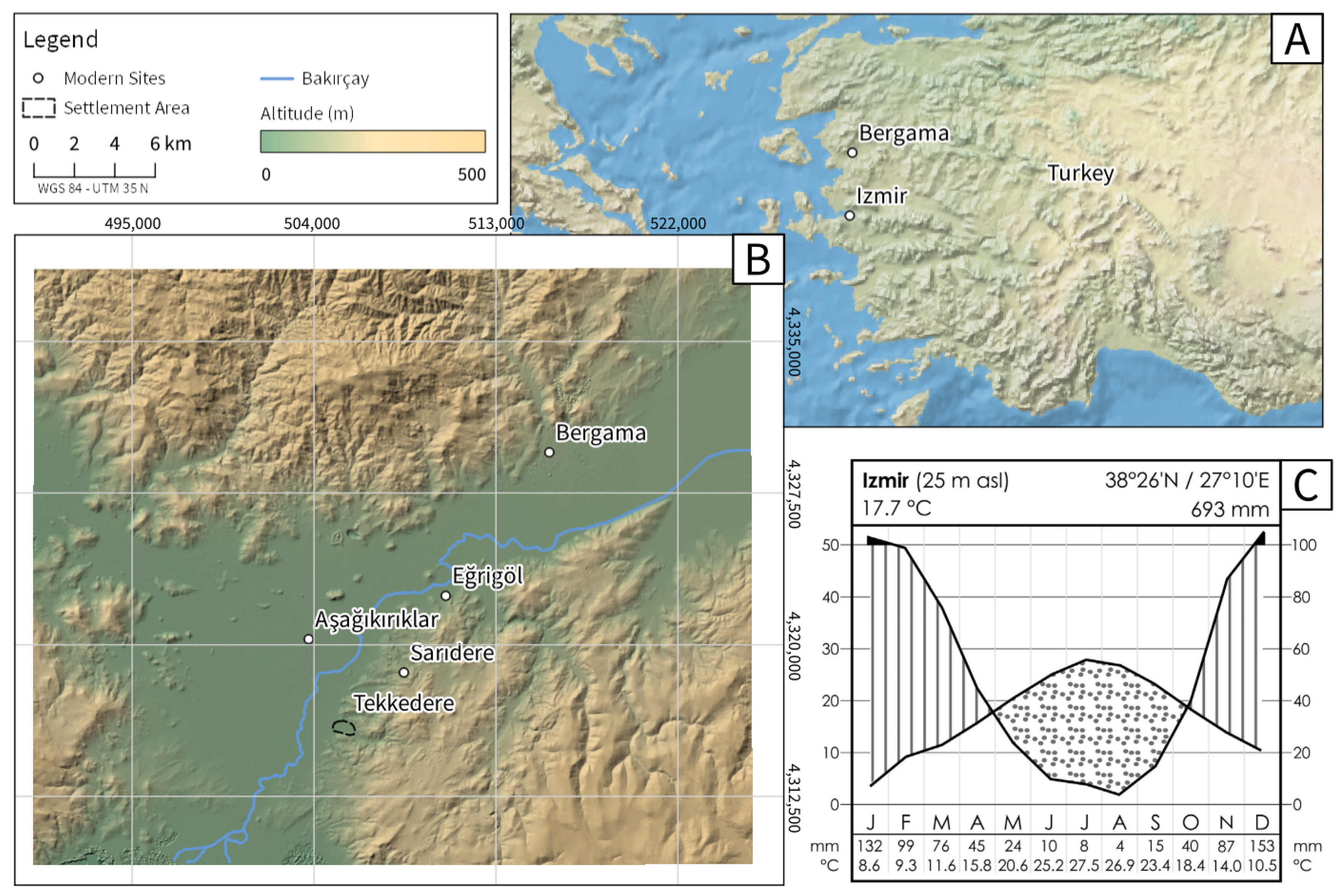
1.3. Study Area
2. Methods
2.1. Biomass Quantification and Dynamics
2.2. Activity Areas
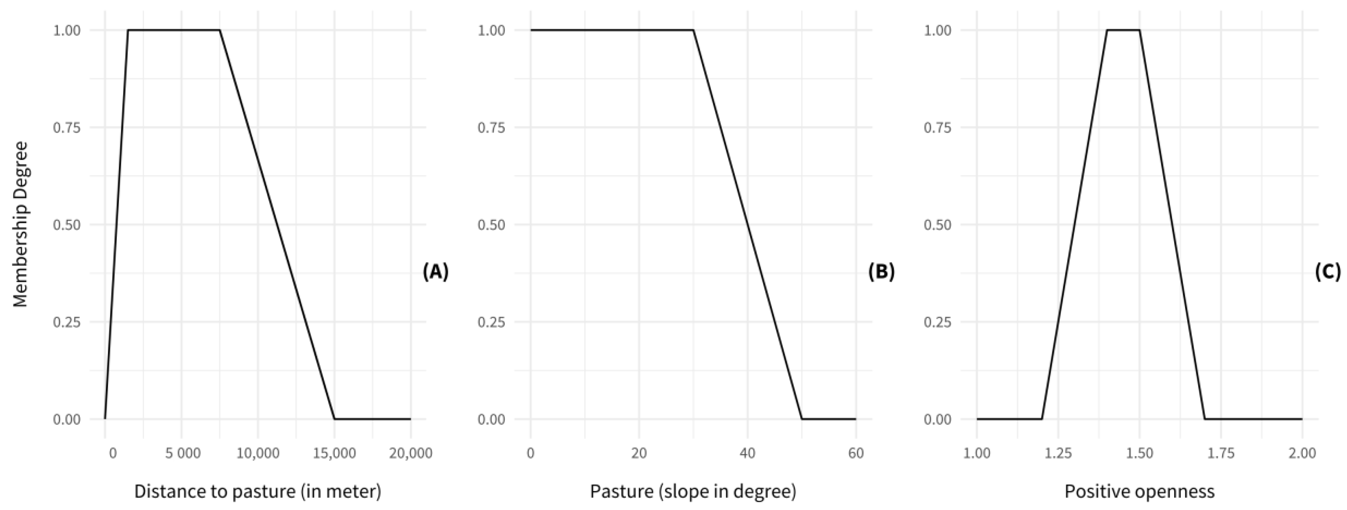
- Pastoralists compete with agricultural production for arable land [60]. According to Forbes [61], p. 101, herders and owners were liable for any damages. Therefore, areas in walking distance of up to 1.5 km from the settlement were assumed to be less suitable, because they might have rather been used for agricultural production than for grazing, and thus would result in potential conflicts between farmers and pastoralists. (Figure 2A; [60]);
- Research on movement patterns of pastoralists in Greece has shown that herders—not considered as nomadic pastoralists—move distances of 10 to 15 km on a daily basis [47]. Therefore, areas in walking distance larger than 15 km were treated as unsuitable, because this distance is too large for the simulated daily short distance pastoralism (Figure 2A);
- Over- and early spring grazing—especially in sloping fields—destroys vegetation and causes erosion, leading to a loss of available pasture areas and biodiversity in general [62]. Slope gradients steeper than 25% lead to a significant increase in soil erosion [63]. Therefore, due to a higher sensitivity to erosion [64], too steep areas were treated as little suitable (Figure 2B);
- Pastoralist herders prefer spots from which they can oversee the surrounding area, and can thus visually control their flocks. Therefore, the Positive Topographic Openness [65] was calculated using SAGA GIS [66]. It is a measure of the portion of a circle that is visible at a certain position along a topographic section (Figure 2C);
- Topographical features also influence microclimate of a grazing spot. Humid conditions favour the occurrence of diseases such as foot rot [67]. For our grazing zones, the connection between terrain features and humid conditions was not considered.
2.3. Agent-Based Model
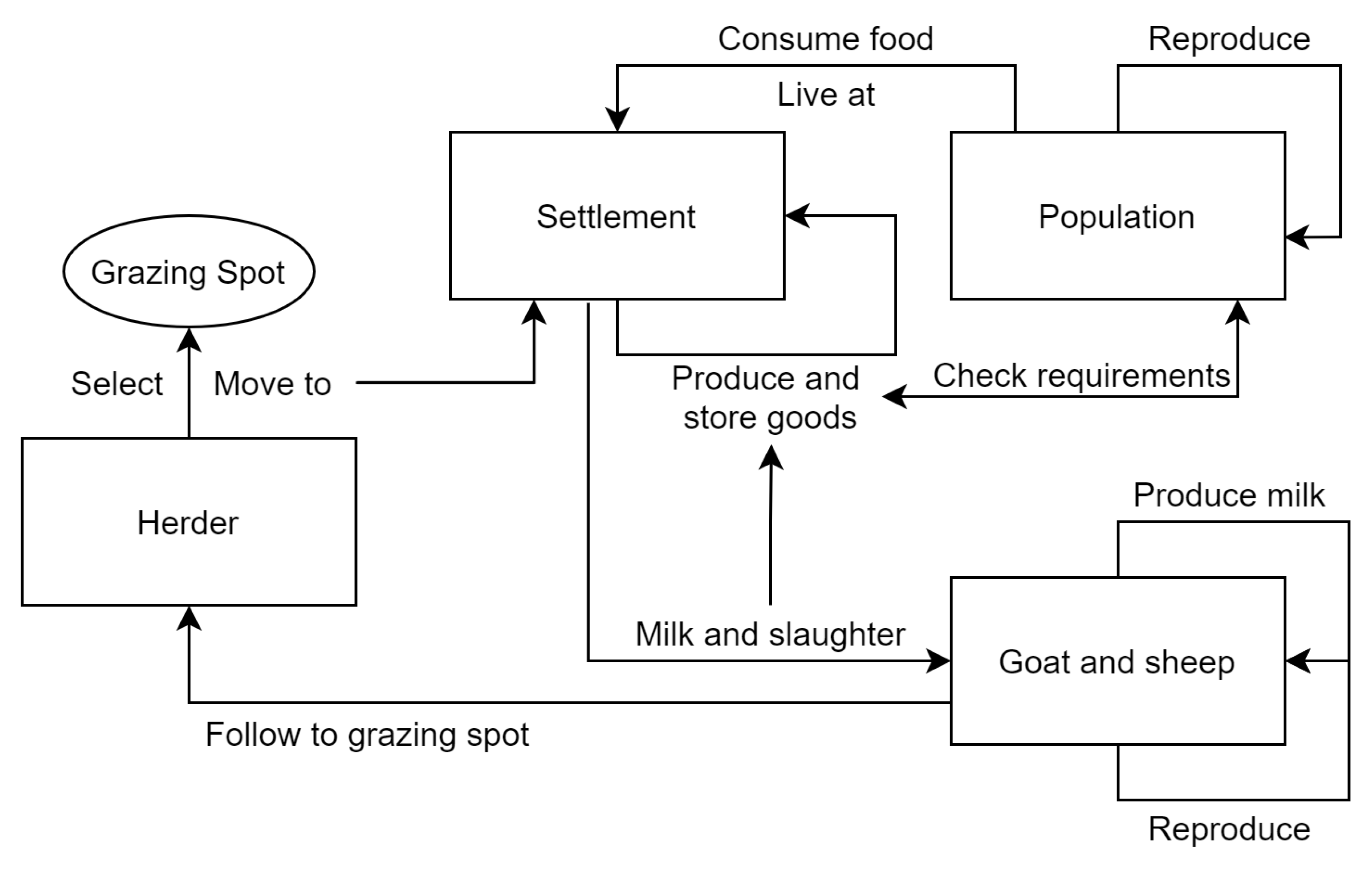
2.3.1. Model Purpose and Agent Types
2.3.2. Demography
2.3.3. Calorie Requirements
2.3.4. Food Consumption
2.3.5. Surplus Goods
2.3.6. Biomass Regrowth
- During this period, the biomass regrow factor per tick is 1.5% of the current value [95]:
- We assume a homogeneous biomass regrowth;
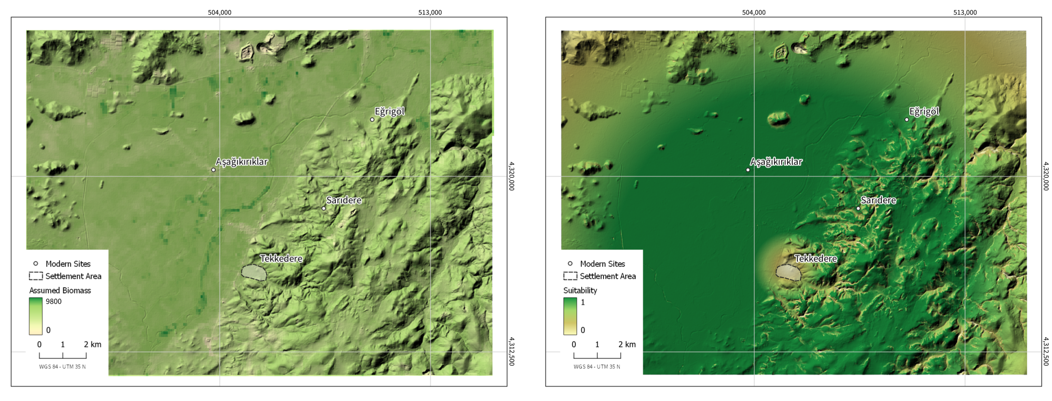
- We further assume that the biomass regrowth is capped by the initial maximum biomass value of c. 9700.
2.4. Modelled Scenarios
3. Results
3.1. Assumed Initial Biomass Distribution and Areas Suitable for Grazing
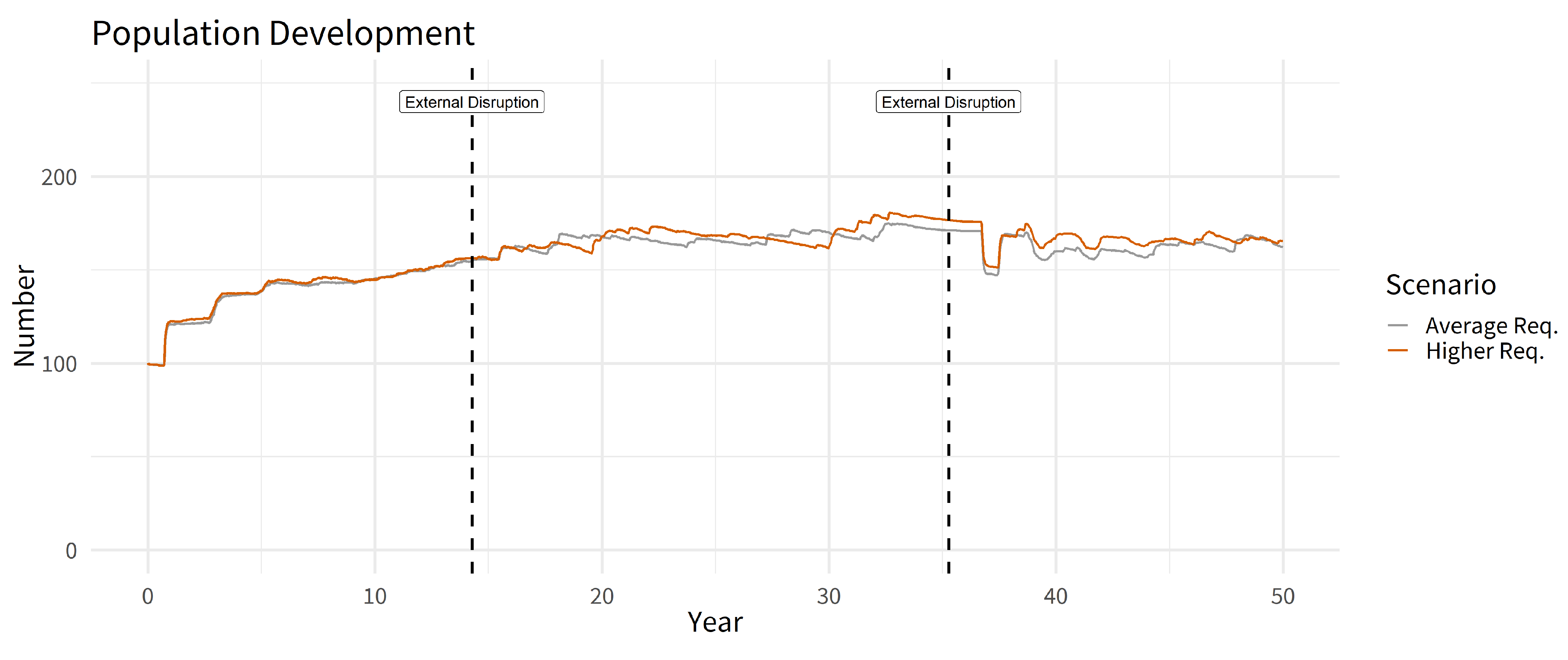
3.2. Population Dynamics
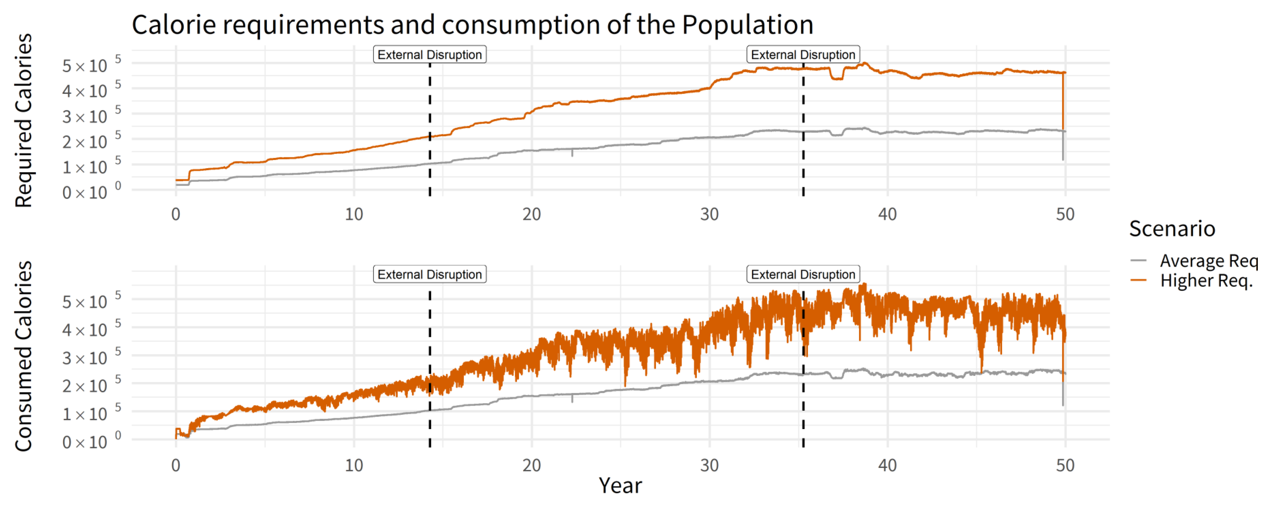
3.3. General Calorie Requirements
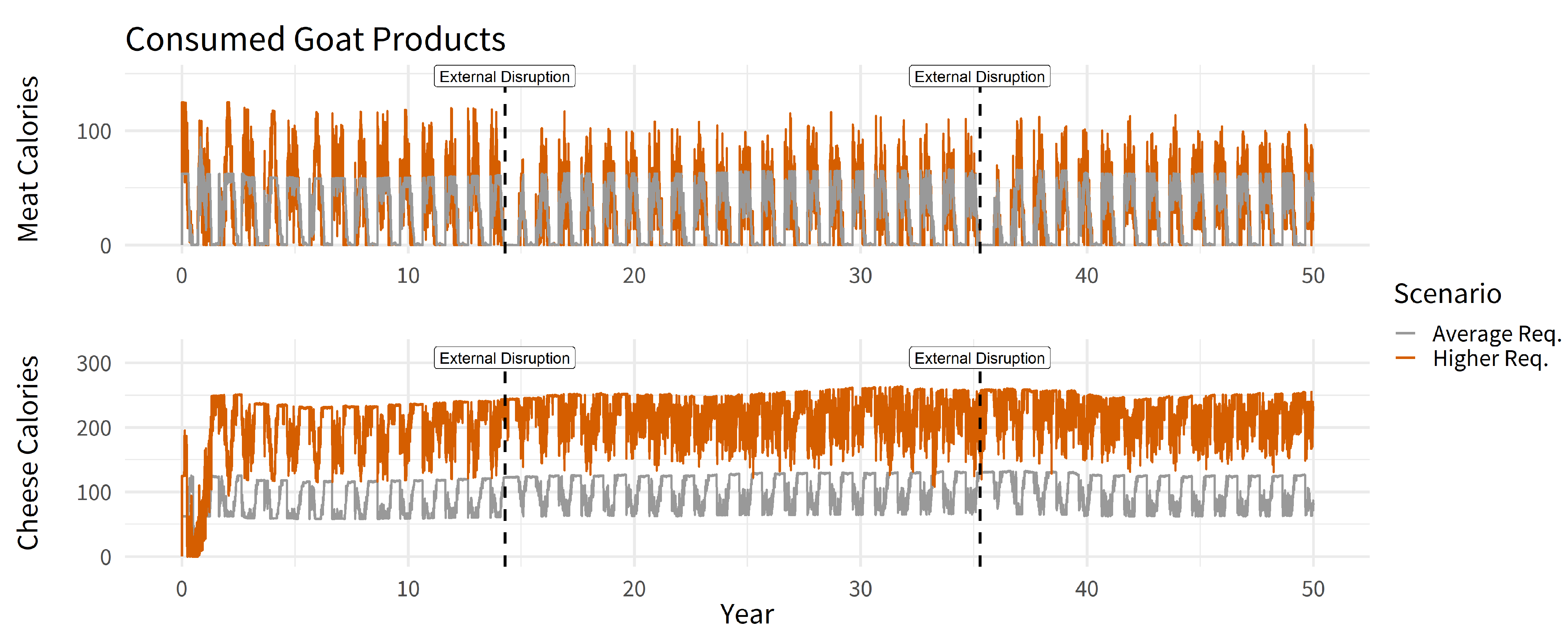
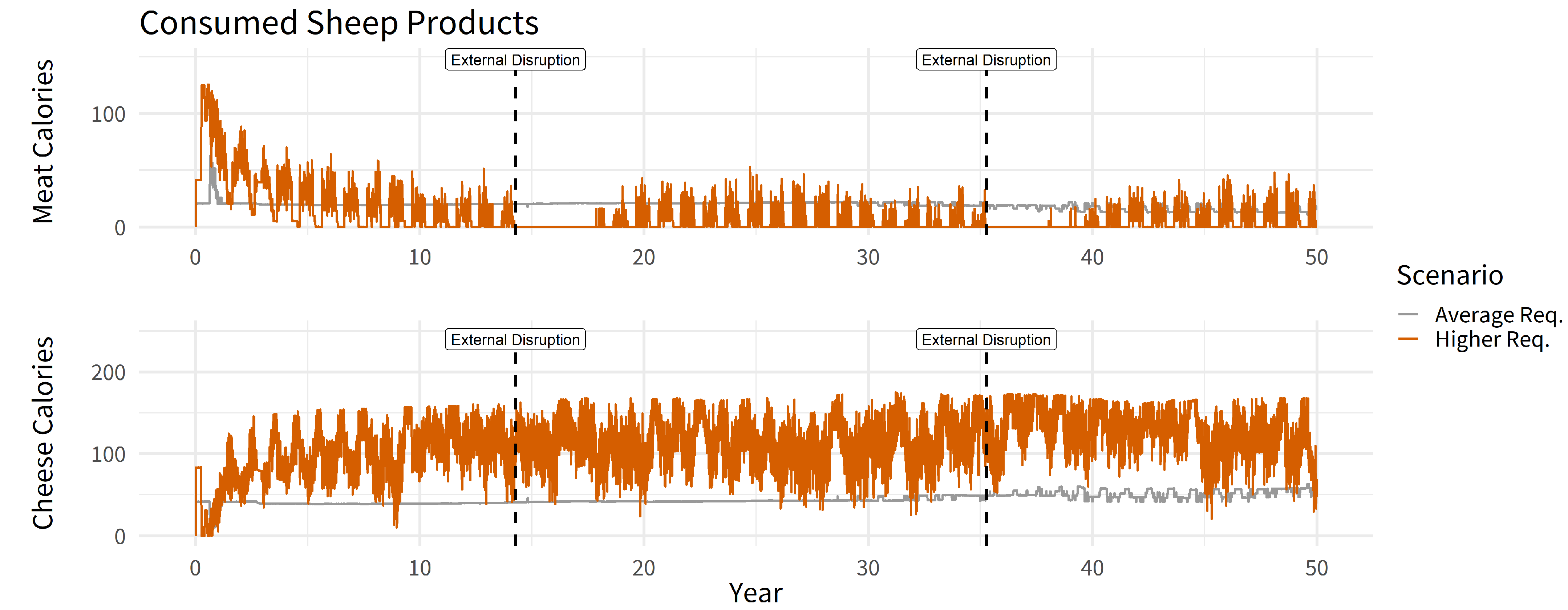
3.4. Coverage of the Calorie Requirements with Goat and Sheep Products
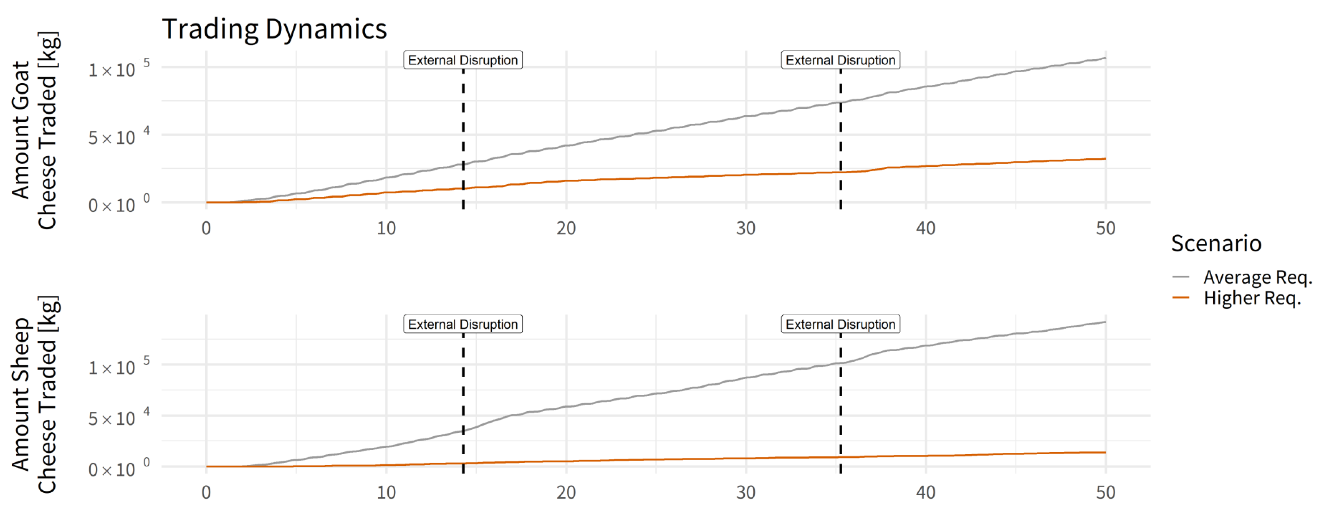
3.5. Trade Dynamics
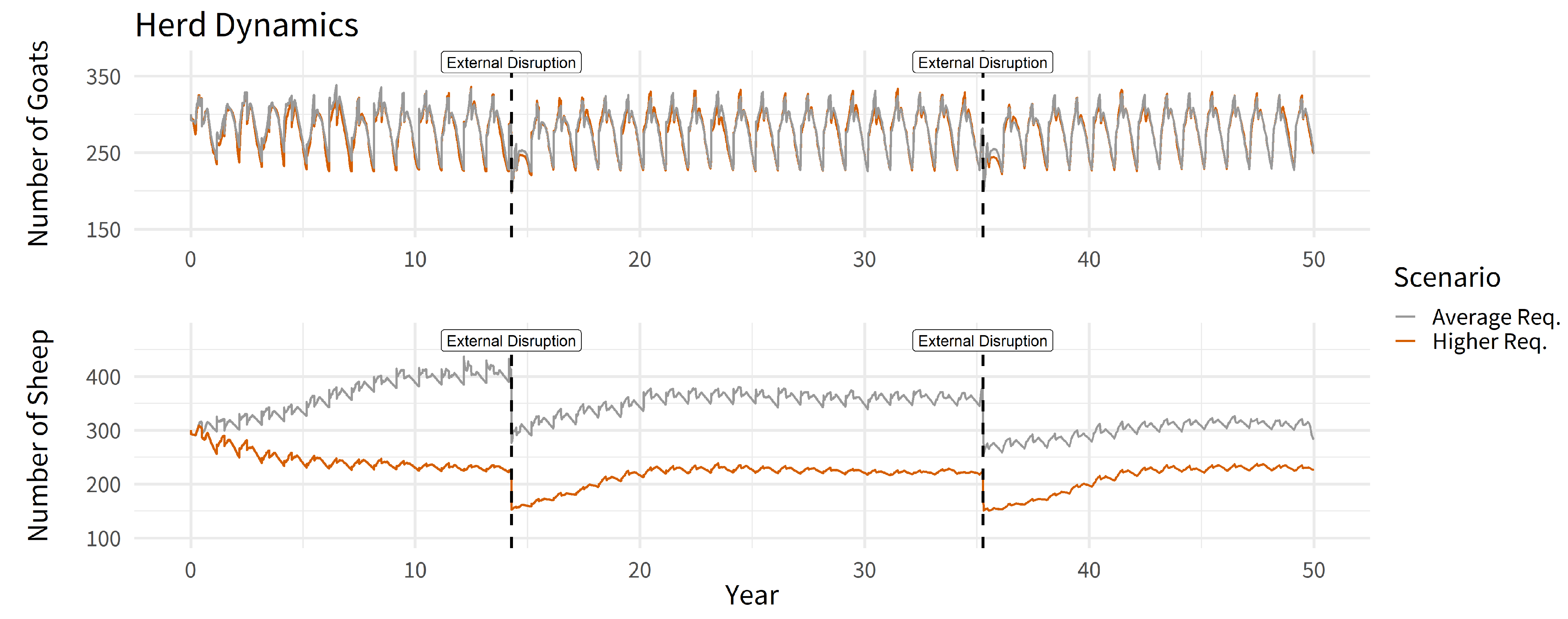
3.6. Herd Dynamics
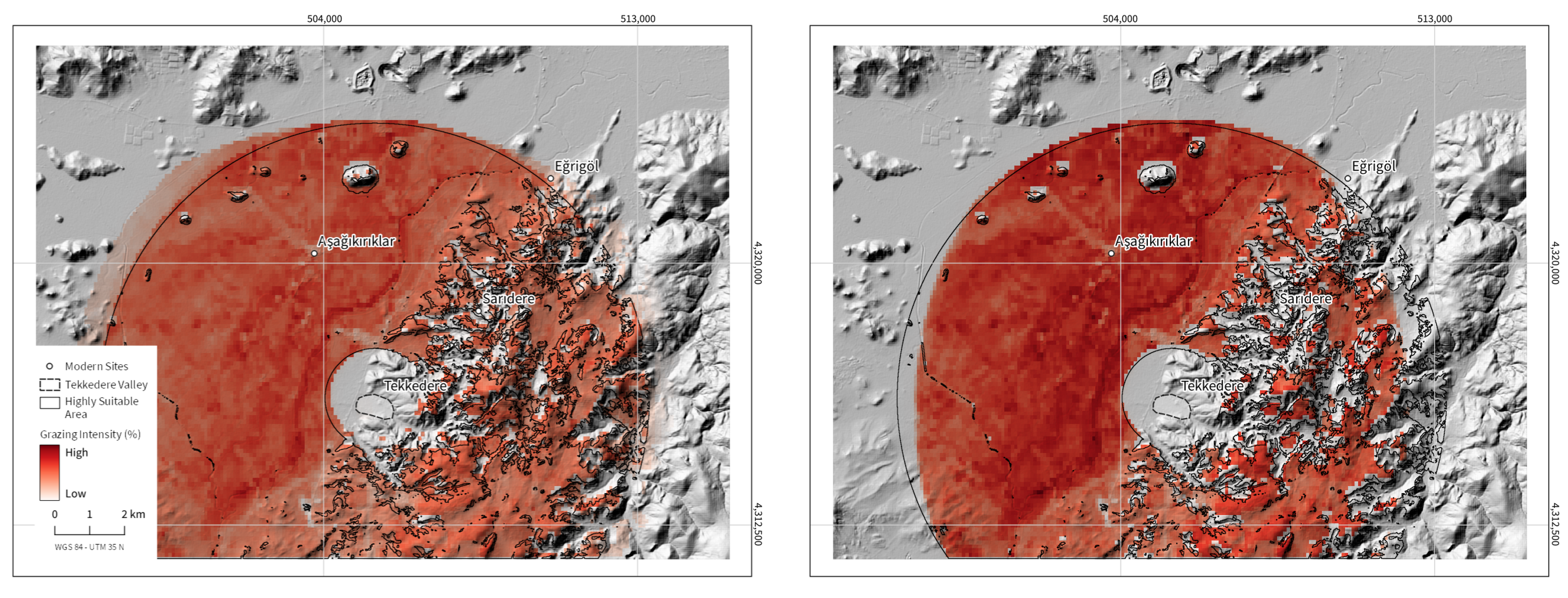
3.7. Grazing Intensity
4. Discussion
4.1. Population Dynamics
4.2. Calorie Requirements and Intake
4.3. Herd Dynamics
4.4. Effects of External Disruptions
4.5. Grazing Patterns
5. Conclusions
Supplementary Materials
Author Contributions
Funding
Institutional Review Board Statement
Informed Consent Statement
Data Availability Statement
Acknowledgments
Conflicts of Interest
References
- Filatova, T.; Verburg, P.H.; Parker, D.C.; Stannard, C.A. Spatial Agent-Based Models for Socio-Ecological Systems: Challenges and Prospects. Environ. Model. Softw. 2013, 45, 1–7. [Google Scholar] [CrossRef]
- Van Schrojenstein Lantman, J.; Verburg, P.H.; Bregt, A.; Geertman, S. Core Principles and Concepts in Land-Use Modelling: A Literature Review. In Land-Use Modelling in Planning Practice; Springer: Amsterdam, The Netherlands, 2011; pp. 35–57. [Google Scholar] [CrossRef]
- Noszczyk, T. A review of approaches to land use changes modeling. Hum. Ecol. Risk Assess. Int. J. 2018, 25, 1377–1405. [Google Scholar] [CrossRef]
- Anderson, J.R. A Land Use and Land Cover Classification System for Use with Remote Sensor Data; US Geological Survey Professional Paper; United States Government Printing Office: Washington, DC, USA, 1976. [Google Scholar]
- Satya, B.A.; Shashi, M.; Deva, P. Future land use land cover scenario simulation using open source GIS for the city of Warangal, Telangana, India. Appl. Geomat. 2020, 12, 281–290. [Google Scholar] [CrossRef]
- White, R.; Engelen, G. Cellular Automata and Fractal Urban Form: A Cellular Modelling Approach to the Evolution of Urban Land-Use Patterns. Environ. Plan. A Econ. Space 1993, 25, 1175–1199. [Google Scholar] [CrossRef]
- Li, X.; Yeh, A.G.O. Neural-network-based cellular automata for simulating multiple land use changes using GIS. Int. J. Geogr. Inf. Sci. 2002, 16, 323–343. [Google Scholar] [CrossRef]
- Wang, T.; Kazak, J.; Han, Q.; de Vries, B. A framework for path-dependent industrial land transition analysis using vector data. Eur. Plan. Stud. 2019, 27, 1391–1412. [Google Scholar] [CrossRef]
- Parker, D.C.; Manson, S.M.; Janssen, M.A.; Hoffmann, M.J.; Deadman, P. Multi-Agent Systems for the Simulation of Land-Use and Land-Cover Change: A Review. Ann. Assoc. Am. Geogr. 2003, 93, 314–337. [Google Scholar] [CrossRef]
- Tong, X.; Feng, Y. A review of assessment methods for cellular automata models of land-use change and urban growth. Int. J. Geogr. Inf. Sci. 2019, 34, 866–898. [Google Scholar] [CrossRef]
- Smajgl, A.; Brown, D.G.; Valbuena, D.; Huigen, M.G. Empirical characterisation of agent behaviours in socio-ecological systems. Environ. Model. Softw. 2011, 26, 837–844. [Google Scholar] [CrossRef]
- Breckling, B. Individual-Based Modelling Potentials and Limitations. Sci. World J. 2002, 2, 1044–1062. [Google Scholar] [CrossRef]
- An, L. Modeling Human Decisions in Coupled Human and Natural Systems: Review of Agent-Based Models. Ecol. Model. 2012, 229, 25–36. [Google Scholar] [CrossRef]
- Sakamoto, T. Computational Research on Mobile Pastoralism Using Agent-Based Modeling and Satellite Imagery. PLoS ONE 2016, 11, e0151157. [Google Scholar] [CrossRef]
- Rodriguez-Lopez, J.M.; Schickhoff, M.; Sengupta, S.; Scheffran, J. Technological and social networks of a pastoralist artificial society: Agent-based modeling of mobility patterns. J. Comput. Soc. Sci. 2021, 4, 681–707. [Google Scholar] [CrossRef]
- Nelson, E.L.; Khan, S.A.; Thorve, S.; Greenough, P.G. Modeling pastoralist movement in response to environmental variables and conflict in Somaliland: Combining agent-based modeling and geospatial data. PLoS ONE 2020, 15, e0244185. [Google Scholar] [CrossRef]
- Dahl, G.; Hjort, A. Having Herds: Pastoral Herd Growth and Household Economy; Stockholm Studies in Social Anthropology No. 2; University of Stockholm: Stockholm, Sweden, 1976. [Google Scholar]
- Lake, M.W. Explaining the Past with ABM: On Modelling Philosophy. In Agent-Based Modeling and Simulation in Archaeology; Springer: Cham, Switzerland, 2015; pp. 3–35. [Google Scholar]
- Müller, D.; Munroe, D.K. Current and future challenges in land-use science. J. Land Use Sci. 2014, 9, 133–142. [Google Scholar] [CrossRef]
- Verburg, P.H.; Dearing, J.A.; Dyke, J.G.; Van Der Leeuw, S.; Seitzinger, S.; Steffen, W.; Syvitski, J. Methods and Approaches to Modelling the Anthropocene. Glob. Environ. Chang. 2016, 39, 328–340. [Google Scholar] [CrossRef]
- Gilbert, N. Agent-Based Models; Sage Publications: Thousand Oaks, CA, USA, 2019; Volume 153. [Google Scholar]
- Dean, J.S.; Gumerman, G.J.; Epstein, J.M.; Axtell, R.L.; Swedlund, A.C.; Parker, M.T.; McCarroll, S. Understanding Anasazi Culture Change through Agent-Based Modeling. In Dynamics in Human and Primate Societies: Agent-Based Modeling of Social and Spatial Processes; Oxford University Press: New York, NY, USA, 2000; pp. 179–205. [Google Scholar]
- Kohler, T.A.; Gumerman, G.J.; Reynolds, R.G. Simulating Ancient Societies. Sci. Am. 2005, 293, 76–84. [Google Scholar] [CrossRef]
- Axtell, R.L.; Epstein, J.M.; Dean, J.S.; Gumerman, G.J.; Swedlund, A.C.; Harburger, J.; Chakravarty, S.; Hammond, R.; Parker, J.; Parker, M. Population Growth and Collapse in a Multiagent Model of the Kayenta Anasazi in Long House Valley. Proc. Natl. Acad. Sci. USA 2002, 99, 7275–7279. [Google Scholar] [CrossRef]
- Barton, C.M.; Ullah, I.; Heimsath, A. How to Make a Barranco: Modeling Erosion and Land-Use in Mediterranean Landscapes. Land 2015, 4, 578–606. [Google Scholar] [CrossRef]
- Barton, C.M.; Ullah, I.; Mitasova, H. Computational modeling and Neolithic socioecological dynamics: A case study from southwest Asia. Am. Antiq. 2010, 364–386. [Google Scholar] [CrossRef]
- Barton, C.M.; Ullah, I.I.; Bergin, S.M.; Mitasova, H.; Sarjoughian, H. Looking for the future in the past: Long-term change in socioecological systems. Ecol. Model. 2012, 241, 42–53. [Google Scholar] [CrossRef]
- Mitasova, H.; Barton, C.; Ullah, I.; Hofierka, J.; Harmon, R. GIS-Based Soil Erosion Modeling. In Treatise on Geomorphology; Academic Press: San Diego, CA, USA, 2013; Volume 3, pp. 228–258. [Google Scholar] [CrossRef]
- Moritz, M.; Hamilton, I.M.; Yoak, A.J.; Scholte, P.; Cronley, J.; Maddock, P.; Pi, H. Simple Movement Rules Result in Ideal Free Distribution of Mobile Pastoralists. Ecol. Model. 2015, 305, 54–63. [Google Scholar] [CrossRef]
- Dressler, G.; Hoffmann, F.; Breuer, I.; Kreuer, D.; Mahdi, M.; Frank, K.; Müller, B. Polarization in (post) nomadic resource use in Eastern Morocco: Insights using a multi-agent simulation model. Reg. Environ. Chang. 2019, 19, 489–500. [Google Scholar] [CrossRef]
- Khazanov, A.M. Nomads and the Outside World; Cambridge University Press: Cambridge, UK, 1984; Volume 167. [Google Scholar]
- Pearson, J.A.; Buitenhuis, H.; Hedges, R.E.; Martin, L.; Russell, N.; Twiss, K.C. New Light on Early Caprine Herding Strategies from Isotope Analysis: A Case Study from Neolithic Anatolia. J. Archaeol. Sci. 2007, 34, 2170–2179. [Google Scholar] [CrossRef]
- Little, M.A. Pastoralism. In Basics in Human Evolution; Academic Press: Boston, MA, USA, 2015; pp. 337–347. [Google Scholar] [CrossRef]
- Salzman, P.C. Pastoralists: Equality, Hierarchy, and The State; Routledge: New York, NY, USA, 2018. [Google Scholar]
- Honeychurch, W.; Makarewicz, C.A. The Archaeology of Pastoral Nomadism. Annu. Rev. Anthropol. 2016, 45, 341–359. [Google Scholar] [CrossRef]
- Yang, X.; Becker, F.; Knitter, D.; Schütt, B. An Overview of the Geomorphological Characteristics of the Pergamon Micro-Region (Bakırçay and Madra River Catchments, Aegean Region, West Turkey). Land 2021, 10, 667. [Google Scholar] [CrossRef]
- Becker, F.; Knitter, D.; Nykamp, M.; Schütt, B. Meta-Analysis of Geomorphodynamics in the Western Lower Bakırçay Plain (Aegean Region, Turkey). Land 2020, 9, 338. [Google Scholar] [CrossRef]
- Turkish Statistical Institute. Population of City, Towns and Villages—2010 (Archived). 2012. Available online: https://web.archive.org/web/20120425074508/http://rapor.tuik.gov.tr/reports/rwservlet?adnksdb2=&ENVID=adnksdb2Env&report=idari_yapi_09sonrasi.RDF&p_il1=35&p_yil=2010&p_dil=2&desformat=html (accessed on 24 February 2021).
- Asuman Karabulut. Bergama District from Tanzimat to the Second Constitutional Era (1839–1908). Ph.D. Thesis, Manisa Celal Bayar University, Manisa, Turkey, 2017. Available online: https://tez.yok.gov.tr/UlusalTezMerkezi/tezDetay.jsp?id=xptOfhsg9KENf96yy6nIxw&no=QWtWLlZPKHTKFGiiIbCnkQ (accessed on 1 March 2021).
- Pirson, F. Pergamon—Das neue Forschungsprogramm und die Arbeiten in der Kampagne 2019. Archäologischer Anzeiger 2021, 2, 2510–4713. [Google Scholar] [CrossRef]
- Pirson, F. Pergamon, Türkei. Pergamon. Die Arbeiten des Jahres 2019. e-Forschungsberichte 2020, 3, 111–121. [Google Scholar]
- Kottek, M.; Grieser, J.; Beck, C.; Rudolf, B.; Rubel, F. World Map of the Köppen-Geiger Climate Classification Updated. Meteorol. Z. 2006, 15, 259–263. [Google Scholar] [CrossRef]
- Lionello, P.; Malanotte-Rizzoli, P.; Boscolo, R.; Alpert, P.; Artale, V.; Li, L.; Luterbacher, J.; May, W.; Trigo, R.; Tsimplis, M.; et al. The Mediterranean Climate: An Overview of the Main Characteristics and Issues. In Developments in Earth and Environmental Sciences; Elsevier: Amsterdam, The Netherlands, 2006; Volume 4, pp. 1–26. [Google Scholar] [CrossRef]
- Schulz, M.; Paul, A. Holocene Climate Variability on Centennial-to-Millennial Time Scales: 1. Climate Records from the North-Atlantic Realm. In Climate Development and History of the North Atlantic Realm; Springer: Berlin/Heidelberg, Germany, 2002; pp. 41–54. [Google Scholar]
- Dusar, B.; Verstraeten, G.; Notebaert, B.; Bakker, J. Holocene Environmental Change and Its Impact on Sediment Dynamics in the Eastern Mediterranean. Earth Sci. Rev. 2011, 108, 137–157. [Google Scholar] [CrossRef]
- Finné, M.; Holmgren, K.; Sundqvist, H.S.; Weiberg, E.; Lindblom, M. Climate in the Eastern Mediterranean, and Adjacent Regions, during the Past 6000 Years–A Review. J. Archaeol. Sci. 2011, 38, 3153–3173. [Google Scholar] [CrossRef]
- Chang, C. Archaeological Landscapes. In Space, Time, and Archaeological Landscapes; Jochim, M., Rossignol, J., Wandsnider, L., Eds.; Springer: Boston, MA, USA, 1992; pp. 65–89. [Google Scholar] [CrossRef]
- Boessneck, J.; von den Driesch, A. Knochenfunde Aus Zisternen in Pergamon; Institut für Palaeoanatomie, Domestikationsforschung und Geschichte der Tiermedizin der Universität München, Deutsches Archäologisches Institut, Abteilung Istanbul: München, Germany, 1985. [Google Scholar]
- Laabs, J.; Knitter, D. How Much Is Enough? First Steps to a Social Ecology of the Pergamon Microregion. Land 2021, 10, 479. [Google Scholar] [CrossRef]
- Pirson, F.; Zimmermann, M. Wirtschaftliche Ressourcen, ländliche Siedlungen und politische Repräsentation. In Pergamon; Grüßinger, R., Kästner, V., Scholl, A., Eds.; Imhof: Petersberg, Germany, 2014; pp. 58–65. [Google Scholar]
- Sträßer, M. Klimadiagramm-Atlas der Erde: Teil 2: Asien, Lateinamerika, Afrika, Australien und Ozeanien, Polarländer. Monats-und Jahresmittelwerte von Temperatur und Niederschlag für den Zeitraum 1961–1990; Duisburger Geographische Arbeiten: Dortmund, Germany, 1999. [Google Scholar]
- Chilonda, P.; Otte, J. Indicators to Monitor Trends in Livestock Production at National, Regional and International Levels. Livest. Res. Rural. Dev. 2006, 18, 117. [Google Scholar]
- Natural Resources Conservation Service (NRCS). Balancing Your Animals with Your Forage–Small Scale Solutions for Your Farm: How Many Animals Should Be on Your Pasture? Available online: https://www.nrcs.usda.gov/Internet/FSE_DOCUMENTS/stelprdb1167344.pdf (accessed on 2 January 2021).
- Von Reden, S.B.; Arbeitszeit. In Der Neue Pauly; Cancik, H., Schneider, H., Landfester, M., Eds.; New Pauly Online, Brill: 2006. Available online: https://referenceworks.brillonline.com/browse/brill-s-new-pauly (accessed on 16 June 2021).
- Suncurves, A.S. Sunrise and Sunset Times for Bergama, Turkey by Suncurves. 2021. Available online: https://www.suncurves.com/en/v/20394/ (accessed on 16 May 2021).
- Hakyemez, B.H.; Gökkuş, A.; Yurtman, I.Y.; Savaş, T. Production Potential of a Natural Pasture Compared to a Wheat Pasture, Both Grazed by Lactating Goats under Mediterranean Climate Conditions. Turk. J. Agric. For. 2008, 32, 501–511. [Google Scholar]
- Albayrak, S.; Türk, M.; Yüksel, O.; Yilmaz, M. Forage Yield and the Quality of Perennial Legume-Grass Mixtures under Rainfed Conditions. Notulae Botanicae Horti Agrobotanici Cluj-Napoca 2011, 39, 114–118. [Google Scholar] [CrossRef]
- Zadeh, L.A. Information and Control. Fuzzy Sets 1965, 8, 338–353. [Google Scholar]
- Hamer, W.; Knitter, D. FuzzyLandscapes–Fuzzy Analyses with a Focus on Raster Data. Zenodo 2018, 30, epub ahead of print. [Google Scholar]
- Chang, C.; Koster, H.A. Beyond bones: Toward an archaeology of pastoralism. In Advances in Archaeological Method and Theory; Academic Press: San Diego, CA, USA, 1986; pp. 97–148. [Google Scholar]
- Forbes, H. Landscape exploitation via pastoralism: Examining the ‘lanscape degradation’ versus sustainable economy debate in the post-Medieval Southern Argolid. In Landscape and Land Use in Postglacial Greece; Halstead, P., Frederick, C., Eds.; Sheffield University Press: Sheffield, UK, 2000; pp. 95–109. [Google Scholar]
- Curebal, I.; Efe, R.; Soykan, A.; Sonmez, S. Impacts of anthropogenic factors on land degradation during the anthropocene in Turkey. J. Environ. Biol. 2015, 36, 51. [Google Scholar]
- Koulouri, M.; Giourga, C. Land abandonment and slope gradient as key factors of soil erosion in Mediterranean terraced lands. Catena 2007, 69, 274–281. [Google Scholar] [CrossRef]
- Panagopoulos, Y.; Dimitriou, E.; Skoulikidis, N. Vulnerability of a Northeast Mediterranean Island to Soil Loss. Can Grazing Management Mitigate Erosion? Water 2019, 11, 1491. [Google Scholar] [CrossRef]
- Yokoyama, R.; Shirasawa, M.; Pike, R.J. Visualizing Topography by Openness: A New Application of Image Processing to Digital Elevation Models. Photogramm. Eng. Remote Sens. 2002, 68, 257–266. [Google Scholar]
- Conrad, O.; Bechtel, B.; Bock, M.; Dietrich, H.; Fischer, E.; Gerlitz, L.; Wehberg, J.; Wichmann, V.; Böhner, J. System for Automated Geoscientific Analyses (SAGA) v. 2.1.4. Geosci. Model Dev. 2015, 8, 1991–2007. [Google Scholar] [CrossRef]
- Angell, J.W.; Grove-White, D.H.; Duncan, J.S. Sheep and farm level factors associated with footrot: A longitudinal repeated cross-sectional study of sheep on six farms in the UK. Vet. Rec. 2018, 182, 293. [Google Scholar] [CrossRef]
- Bezanson, J.; Edelman, A.; Karpinski, S.; Shah, V.B. Julia: A fresh approach to numerical computing. SIAM Rev. 2017, 59, 65–98. [Google Scholar] [CrossRef]
- Datseris, G.; Vahdati, A.R.; DuBois, T.C. Agents.jl: A performant and feature-full agent based modelling software of minimal code complexity. arXiv 2021, arXiv:cs.MA/2101.10072. [Google Scholar]
- Quinn, J. CSV.jl. 2021. Available online: https://github.com/JuliaData/CSV.jl (accessed on 9 November 2020).
- Anthoff, D. CSVFiles.jl. 2021. Available online: https://github.com/queryverse/CSVFiles.jl (accessed on 9 November 2020).
- White, J.M.; Kamiński, B. DataFrames.jl. 2021. Available online: https://github.com/JuliaData/DataFrames.jl (accessed on 9 November 2020).
- Pronk, M. GeoArrays.jl. 2021. Available online: https://github.com/evetion/GeoArrays.jl (accessed on 9 November 2020).
- Grimm, V.; Railsback, S.F.; Vincenot, C.E.; Berger, U.; Gallagher, C.; DeAngelis, D.L.; Edmonds, B.; Ge, J.; Giske, J.; Groeneveld, J.; et al. The ODD Protocol for Describing Agent-Based and Other Simulation Models: A Second Update to Improve Clarity, Replication, and Structural Realism. J. Artif. Soc. Soc. Simul. 2020, 23, 7. [Google Scholar] [CrossRef]
- Datseris, G.; Isensee, J.; Pech, S.; Gál, T. DrWatson: The perfect sidekick for your scientific inquiries. J. Open Source Softw. 2020, 5, 2673. [Google Scholar] [CrossRef]
- Kluge, N. Sexualverhalten Jugendlicher Heute: Ergebnisse einer Repräsentativen Jugend-und Elternstudie über Verhalten und Einstellungen zur Sexualität; Juventa-Verlag: München, Germany, 1998. [Google Scholar]
- Mulder, M.B. Demography of Pastoralists: Preliminary Data on the Datoga of Tanzania. Hum. Ecol. 1992, 20, 383–405. [Google Scholar] [CrossRef]
- Yilmaz, H.; Cripps, P.; Turan, N.; Ozgur, N.; Green, L.; Anil, M.; Ilgaz, A.; Morgan, K. A postal survey of abortion in Turkish sheep. Small Rumin. Res. 2002, 45, 151–158. [Google Scholar] [CrossRef]
- Hughes, R.; Weiberg, E.; Bonnier, A.; Finné, M.; Kaplan, J. Quantifying Land Use in Past Societies from Cultural Practice and Archaeological Data. Land 2018, 7, 9. [Google Scholar] [CrossRef]
- Borgerhoff Mulder, M.; Fazzio, I.; Irons, W.; McElreath, R.L.; Bowles, S.; Bell, A.; Hertz, T.; Hazzah, L. Pastoralism and Wealth Inequality: Revisiting an Old Question. Curr. Anthropol. 2010, 51, 35–48. [Google Scholar] [CrossRef]
- Arbuckle, B.S.; Hammer, E.L. The Rise of Pastoralism in the Ancient Near East. J. Archaeol. Res. 2019, 27, 391–449. [Google Scholar] [CrossRef]
- Degen, A. Sheep and goat milk in pastoral societies. Small Rumin. Res. 2007, 68, 7–19. [Google Scholar] [CrossRef]
- Kamber, U. The Traditional Cheeses of Turkey: Cheeses Common to All Regions. Food Rev. Int. 2007, 24, 1–38. [Google Scholar] [CrossRef]
- Beltrán-Sánchez, H.; Crimmins, E.M.; Finch, C.E. Early cohort mortality predicts the rate of aging in the cohort: A historical analysis. J. Dev. Orig. Health Dis. 2012, 3, 380–386. [Google Scholar] [CrossRef]
- Brown, L. Pastoral People and Conservation. In Conservation for Survival-Ethiopia’s Choice; Haile Selassie Press: Addis Ababa, Ethiopia, 1973; pp. 67–76. [Google Scholar]
- U.S. Department of Agriculture (USDA). Estimated Calorie Needs per Day by Age, Gender, and Physical Activity Level. 2011. Available online: https://fns-prod.azureedge.net/sites/default/files/usda_food_patterns/EstimatedCalorieNeedsPerDayTable.pdf (accessed on 24 February 2021).
- Thomson, A.M.; Hytten, F.E. Calorie requirements in human pregnancy. Proc. Nutr. Soc. 1961, 20, 76–83. [Google Scholar] [CrossRef]
- Pettegrew, D.K. Chasing the Classical Farmstead: Assessing the Formation and Signature of Rural Settlement in Greek Landscape Archaeology. J. Mediterr. Archaeol. 2001, 14, 189–209. [Google Scholar] [CrossRef]
- Bintliff, J.; Farinetti, E.; Howard, P.; Sarri, K.; Sbonias, K. Classical farms, hidden prehistoric landscapes and Greek rural survey: A response and an update. J. Mediterr. Archaeol. 2002, 15, 259–265. [Google Scholar] [CrossRef]
- Ertug-Yaras, F. An Ethnoarchaeological Study of Subsistence and Plant Gathering in Central Anatolia. Ph.D. Thesis, Washington University, St. Louis, MO, USA, 1997. [Google Scholar]
- Ligt, L.D. Fairs and Markets in the Roman Empire: Economic and Social Aspects of Periodic Trade in a Pre-Industrial Society; Number v. 11 in Dutch Monographs on Ancient History and Archaeology; Gieben, J.C., Ed.; Brill Academic Publishers: Leiden, The Netherlands, 1993. [Google Scholar]
- National Geographic. Growing Season. 2011. Available online: http://www.nationalgeographic.org/encyclopedia/growing-season/ (accessed on 15 March 2021).
- Atalay, İ. Vegetation Geography of Turkey; Ege Üniversitesi Basimevi Bornova: Izmir, Turkey, 1994. (In Turkish) [Google Scholar]
- Taner, S.; Sedat, A.; Meral, A. Evaluation of the vegetation period according to climate change scenarios: A case study in the inner west Anatolia subregion of Turkey. Coğrafya Dergisi 2019, 39, 29–39. [Google Scholar]
- Cioffi-Revilla, C.; Rogers, J.D.; Latek, M. The MASON HouseholdsWorld Model of Pastoral Nomad Societies. In Simulating Interacting Agents and Social Phenomena; Takadama, K., Cioffi-Revilla, C., Deffuant, G., Eds.; Springer: Tokyo, Japan, 2010; pp. 193–204. [Google Scholar] [CrossRef]
- Fick, S.E.; Hijmans, R.J. WorldClim 2: New 1-Km Spatial Resolution Climate Surfaces for Global Land Areas: New Climate Surfaces for Global Land Areas. Int. J. Climatol. 2017, 37, 4302–4315. [Google Scholar] [CrossRef]
- Bottema, S.; Geigle, F. Vorderer Orient, Vegetation im Frühholozän (ca. 8000 BP). In Tübinger Atlas des Vorderen Orients; Reichert: Wiesbaden, Germany, 1990. [Google Scholar]
- Hughes, J.D.; Stoll, M.R. (Eds.) The Mediterranean; Nature and Human Societies, ABC-CLIO: Santa Barbara, CA, USA, 2005. [Google Scholar]
- Rizzoli, P.; Martone, M.; Gonzalez, C.; Wecklich, C.; Tridon, D.B.; Bräutigam, B.; Bachmann, M.; Schulze, D.; Fritz, T.; Huber, M.; et al. Generation and performance assessment of the global TanDEM-X digital elevation model. ISPRS J. Photogramm. Remote Sens. 2017, 132, 119–139. [Google Scholar] [CrossRef]
- Wessel, B.; Huber, M.; Wohlfart, C.; Marschalk, U.; Kosmann, D.; Roth, A. Accuracy assessment of the global TanDEM-X Digital Elevation Model with GPS data. ISPRS J. Photogramm. Remote Sens. 2018, 139, 171–182. [Google Scholar] [CrossRef]
- Goodchild, H.; Witcher, R. Modelling the agricultural landscapes of Republican Italy. In Agricoltura E Scambi Nell’italia Tardo Repubblicana; Carlsen, J., Cascio, E.L., Eds.; Edipuglia: Rome/Bari, Italy, 2010; pp. 187–220. [Google Scholar]
- Halstead, P. Pastoralism or Household Herding? Problems of Scale and Specialization in Early Greek Animal Husbandry. World Archaeol. 1996, 28, 20–42. [Google Scholar] [CrossRef]
- Arbuckle, B.S.; Atici, L. Initial Diversity in Sheep and Goat Management in Neolithic South-Western Asia. Levant 2013, 45, 219–235. [Google Scholar] [CrossRef]
- Vigne, J.D.; Gourichon, L.; Helmer, D.; Martin, L.; Peters, J. The Beginning of Animal Domestication and Husbandry in Southwest Asia. In Quaternary of the Levant, 1st ed.; Enzel, Y., Bar-Yosef, O., Eds.; Cambridge University Press: Cambridge, UK, 2017; pp. 753–760. [Google Scholar] [CrossRef]
- Lenfers, U.A.; Weyl, J.; Clemen, T. Firewood Collection in South Africa: Adaptive Behavior in Social-Ecological Models. Land 2018, 7, 97. [Google Scholar] [CrossRef]
- Moritz, M.; Buffington, A.; Yoak, A.J.; Hamilton, I.M.; Garabed, R. No Magic Number: An Examination of the Herd-Size Threshold in Pastoral Systems Using Agent-Based Modeling. Hum. Ecol. 2017, 45, 525–532. [Google Scholar] [CrossRef]
- White, S. A model disaster: From the great Ottoman panzootic to the cattle plagues of early modern Europe. In Plague and Contagion in the Islamic Mediterranean; ARC, Amsterdam University Press: The Netherlands, 2017; pp. 91–116. [Google Scholar] [CrossRef]
- Fryxell, J.M.; Sinclair, A.R.E. Seasonal Migration by White-Eared Kob in Relation to Resources. Afr. J. Ecol. 1988, 26, 17–31. [Google Scholar] [CrossRef]
- Thevenin, M. Kurdish Transhumance: Pastoral Practices in South-East Turkey. Pastor. Res. Policy Pract. 2011, 1, 23. [Google Scholar] [CrossRef]
- Makarewicz, C.A.; Arbuckle, B.S.; Öztan, A. Vertical Transhumance of Sheep and Goats Identified by Intra-Tooth Sequential Carbon (δ13C) and Oxygen (δ18O) Isotopic Analyses: Evidence from Chalcolithic Köşk Höyük, Central Turkey. J. Archaeol. Sci. 2017, 86, 68–80. [Google Scholar] [CrossRef]
- Hammer, E.L.; Arbuckle, B.S. 10,000 Years of Pastoralism in Anatolia: A Review of Evidence for Variability in Pastoral Lifeways. Nomadic Peoples 2017, 21, 214–267. [Google Scholar] [CrossRef]
- Fuller, B.T.; De Cupere, B.; Marinova, E.; Van Neer, W.; Waelkens, M.; Richards, M.P. Isotopic Reconstruction of Human Diet and Animal Husbandry Practices during the Classical-Hellenistic, Imperial, and Byzantine Periods at Sagalassos, Turkey. Am. J. Phys. Anthropol. 2012, 149, 157–171. [Google Scholar] [CrossRef]
- Gelasakis, A.; Kalogianni, A.; Bossis, I. Aetiology, Risk Factors, Diagnosis and Control of Foot-Related Lameness in Dairy Sheep. Animals 2019, 9, 509. [Google Scholar] [CrossRef]
- Reu, J.D.; Bourgeois, J.; Bats, M.; Zwertvaegher, A.; Gelorini, V.; Smedt, P.D.; Chu, W.; Antrop, M.; Maeyer, P.D.; Finke, P.; et al. Application of the topographic position index to heterogeneous landscapes. Geomorphology 2013, 186, 39–49. [Google Scholar] [CrossRef]
- Robinson, D.T.; Vittorio, A.D.; Alexander, P.; Arneth, A.; Barton, C.M.; Brown, D.G.; Kettner, A.; Lemmen, C.; O’Neill, B.C.; Janssen, M.; et al. Modelling feedbacks between human and natural processes in the land system. Earth Syst. Dyn. 2018, 9, 895–914. [Google Scholar] [CrossRef]
- Wissenschaftlicher Beirat der Bundesregierung Globale Umweltveränderungen. Welt im Wandel: Die Gefährdung der Böden: Jahresgutachten 1994; Economica Verlag: Bonn, Germany, 1994. [Google Scholar]


| Product | Amount (Unit) |
|---|---|
| Goat Cheese | 300 (kg) |
| Sheep Cheese | 300 (kg) |
| Goat Meat | 300 (kg) |
| Sheep Meat | 300 (kg) |
| Goat Milk | 300 (L) |
| Sheep Milk | 300 (L) |
| Product | Proportion (%) per Scenario | |
|---|---|---|
| Average Requirements | Higher Requirements | |
| Goat Meat | 3.00 | 6.00 |
| Sheep Meat | 1.00 | 2.00 |
| Goat Cheese | 3.00 | 6.00 |
| Sheep Cheese | 2.00 | 4.00 |
| Agent Type | Initial Number |
|---|---|
| Settlement | 1 |
| Population | 100 |
| Herder | 3 |
| Goat | 300 |
| Sheep | 300 |
| Type | Proportion (%) per Scenario | Data from | Differences | ||
|---|---|---|---|---|---|
| Average req. | Higher req. | Dahl and Hjort [17], p. 96 | Average req. | Higher req. | |
| Male Goats | 12.3 | 19.6 | 23.6 | 11.3 | 4.0 |
| Female Goats | 87.7 | 76.4 | 80.4 | −11.3 | −4.0 |
| Juvenile Goats | 20.3 | 20.4 | 33.3 | 13.0 | 12.9 |
| Male Sheep | 8.6 | 60.9 | 22.2 | 13.6 | −38.7 |
| Female Sheep | 91.4 | 39.1 | 77.8 | −13.6 | 38.7 |
| Juvenile Sheep | 10.0 | 7.5 | 22.2 | 12.2 | 14.7 |
Publisher’s Note: MDPI stays neutral with regard to jurisdictional claims in published maps and institutional affiliations. |
© 2021 by the authors. Licensee MDPI, Basel, Switzerland. This article is an open access article distributed under the terms and conditions of the Creative Commons Attribution (CC BY) license (https://creativecommons.org/licenses/by/4.0/).
Share and Cite
Günther, G.; Clemen, T.; Duttmann, R.; Schütt, B.; Knitter, D. Of Animal Husbandry and Food Production—A First Step towards a Modular Agent-Based Modelling Platform for Socio-Ecological Dynamics. Land 2021, 10, 1366. https://doi.org/10.3390/land10121366
Günther G, Clemen T, Duttmann R, Schütt B, Knitter D. Of Animal Husbandry and Food Production—A First Step towards a Modular Agent-Based Modelling Platform for Socio-Ecological Dynamics. Land. 2021; 10(12):1366. https://doi.org/10.3390/land10121366
Chicago/Turabian StyleGünther, Gerrit, Thomas Clemen, Rainer Duttmann, Brigitta Schütt, and Daniel Knitter. 2021. "Of Animal Husbandry and Food Production—A First Step towards a Modular Agent-Based Modelling Platform for Socio-Ecological Dynamics" Land 10, no. 12: 1366. https://doi.org/10.3390/land10121366
APA StyleGünther, G., Clemen, T., Duttmann, R., Schütt, B., & Knitter, D. (2021). Of Animal Husbandry and Food Production—A First Step towards a Modular Agent-Based Modelling Platform for Socio-Ecological Dynamics. Land, 10(12), 1366. https://doi.org/10.3390/land10121366