A Slight Temperature Warming Trend Occurred over Lake Ontario from 2001 to 2018

Abstract

Satellite-derived lake surface water temperature (LSWT) measurements can be used for monitoring purposes. However, analyses based on the LSWT of Lake Ontario and the surrounding land surface temperature (LST) are scarce in the current literature. First, we provide an evaluation of the commonly used Moderate Resolution Imaging Spectroradiometer (MODIS)-derived LSWT/LST (MOD11A1 and MYD11A1) using in situ measurements near the area of where Lake Ontario, the St. Lawrence River and the Rideau Canal meet. The MODIS datasets agreed well with ground sites measurements from 2015–2017, with an R² consistently over 0.90. Among the different ground measurement sites, the best results were achieved for Hill Island, with a correlation of 0.99 and centered root mean square difference (RMSD) of 0.73 K for Aqua/MYD nighttime. The validated MODIS datasets were used to analyze the temperature trend over the study area from 2001 to 2018, through a linear regression method with a Mann–Kendall test. A slight warming trend was found, with 95% confidence over the ground sites from 2003 to 2012 for the MYD11A1-Night datasets. The warming trend for the whole region, including both the lake and the land, was about 0.17 K year⁻¹ for the MYD11A1 datasets during 2003–2012, whereas it was about 0.06 K year⁻¹ during 2003–2018. There was also a spatial pattern of warming, but the trend for the lake region was not obviously different from that of the land region. For the monthly trends, the warming trends for September and October from 2013 to 2018 are much more apparent than those of other months.

1. Introduction

Lakes are always considered as effective and valid sentinels in relation to climate change. They can provide accurate indications for climate change analysis and its regulation [1,2,3,4,5]. However, some of the indicators, such as the lake surface water temperature (LSWT), which could be acquired by various methods, ranging from ground observations to satellite observations and numerical measurements, have not been thoroughly analyzed [6] due to various reasons. For example, sites used in ground networks are not representative of the neighboring locations [7], and there are many lake and weather related uncertainties in estimates from remote sensing. Nevertheless, remote sensing-based observations have gained increasing popularity for analyzing LSWT and have been used as a good proxy indicators for studying the impact of climate change by providing spatial and temporal temperature observations on lake surfaces [6,8].

The 2013 Intergovernmental Panel on Climate Change (IPCC) and some researchers claimed that the world is in a warming hiatus [9,10,11]. Early studies claimed that the global warming hiatus occurred during 1998 to 2012 [11,12], whereas recent studies have claimed the warming rate remained slow into the early 2010s [12]. However, not many details have been revealed through in situ or satellite observations. Fyfe et al. [13] found the recently observed global warming trend is less than that predicted from climate models. The warming hiatus in areas over the world has attracted researchers’ interest. Meanwhile, some researchers debated about whether the warming was on a “hiatus” or “slowed down” [14,15,16].

In 2019, Cheng et al. [17] claimed that the observation-based measurements show a rapid warming of the Earth’s oceans over the past few decades. How fast is Earth warming? What happened in specific parts of the world and with the various land/water surface types? Is there any possibility that we can use satellite-derived surface datasets themselves for warming trend analysis when the air temperature is not available?

The IPCC has also emphasized that the urgent need for long term satellite-derived land surface temperature (LST) (also known as surface skin temperature) data in global warming studies to improve the limits of near surface (2 m) air temperature observations [18]. The relationships between air temperature and surface temperature have been explored on daily and annual bases [19,20]. The daily minimum and maximum air temperatures could be acquired both from ground observations at meteorological stations and from geostationary satellite data through an empirical multiple-linear regression model [7]. Some researchers [21,22] also concluded that the relationships between surface temperature and air temperature are strongest during summer and autumn. Additionally, some studies showed that there was a high correlation between air temperature and surface temperature [18].

Lake Ontario is one of the Great Lakes of North America [23], and there are many big cities around it. The spatial and seasonal trends of Great Lake LSWT have significant impacts on regional and global water management and climate analysis [24]. Nalley et al. [25] used the monthly temperature datasets and concluded that a warming trend occurred in the southern of Ontario due to winter and summer warming, caused by the increases in dew point, air moisture, humidity and the urban heat island effects. They also found that the northern hemisphere has been experiencing more warming since the 1950s than in the southern hemisphere. The importance of Lake Ontario to North America and Earth is obvious. Mohsin et al. [26] used the sequential Mann–Kendall (SQMK) test to conclude that winter is contributing the most to the increase in annual minimum temperature in the Greater Toronto Area (GTA) on the shore of Lake Ontario. In addition, a gradually increasing temperature has been observed in western Canada during last few decades, and it is projected to increase into the mid-century [27,28,29].

Nevertheless, LSWT validation with MODIS surface temperature products and time series trend analysis for Canada have not been thoroughly studied for recent years, especially for inland water and lakes. The Moderate Resolution Imaging Spectroradiometer (MODIS) LSWT product has been validated for many places on Earth through a number of studies [8,30,31,32,33]. However, the quality and feasibility of the satellite retrievals in the different study areas along with systematic errors are also important in the LSWT trend analysis, evaporation and water surface energy flux analysis [34,35,36]. How the satellite-derived products could support the global trend evaluation for the long-term and how the satellite datasets could be used to fill the spatial and temporal gaps of in situ measurements in the Lake Ontario region are challenges for remote sensing researchers [17].

Therefore, this research intended to investigate the feasibility and potential of the MODIS-derived surface temperature products for warming trend analysis over Lake Ontario and its surroundings in eastern Ontario region. This paper first gives an evaluation of the relationships between the current commonly used MODIS-derived LSWT and the in situ measurements from the area near where Lake Ontario, St. Lawrence River and the Rideau Canal meet during the flooding seasons over 2015–2017. Then, the MODIS LSWT datasets obtained from 2001–2018 were used for LSWT recent trend analysis using the linear regression method with Mann–Kendall (MK) testing. Based on the validation and trend analysis, the MODIS data’s compatibility and capability are discussed.

2. Study Area and Data

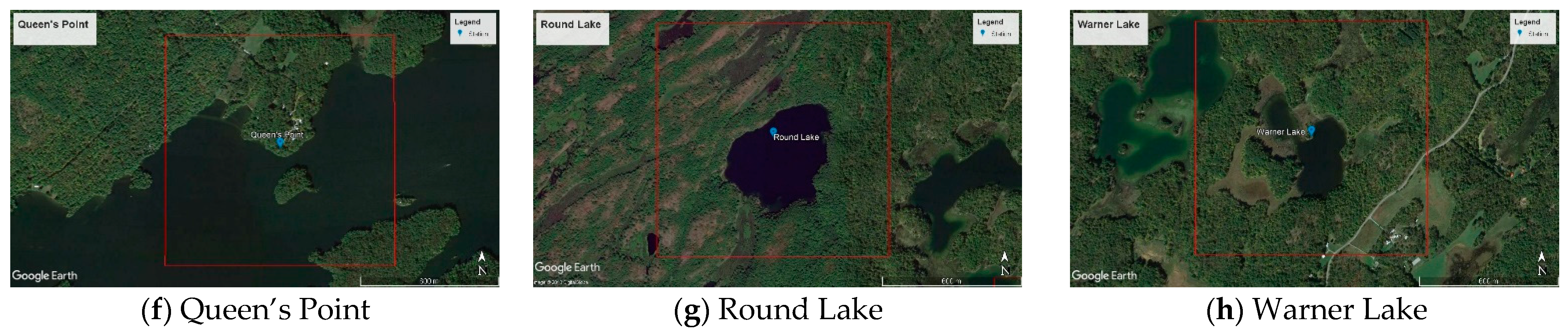
2.1. Study Area

Lake Ontario, one of the Great Lakes, which encompasses between 42.94–45.25° N and 80.46–75.44° W, including Lake Ontario, most of the large Canadian cities and most of the population in Canada was our study area. The average depth and total basin area of Lake Ontario are 86 m and 82,990 km², respectively [24].

The six validation sites are located in and near lakes around where Lake Ontario, Rideau Canal and St. Lawrence River meet. Rideau Canal is an inland waterway between the Canadian capital of Ottawa and Lake Ontario at Kingston, Ontario, where the St. Lawrence River begins. There are many inland lakes and water bodies within this region. The land cover map of Lake Ontario and the six enlarged and specified validation sites are presented in Figure 1 (2017). The land cover map was obtained from MODIS land cover product from the Application for Extracting and Exploring Analysis Ready Samples (AppEEARS). The enlarged picture details the six ground sites around, surrounding Kingston, around the Lake Ontario outlet, St. Lawrence River, in southeastern Ontario, Canada. The six specified validations images were downloaded from Google Earth. It can be clearly seen in the ground sites images that all the validation sites are all covered with vegetation or water. Although the cover is not homogeneous, it can largely meet the validation criterion.

2.2. MODIS Datasets

MODIS, acquiring data in 36 spectral bands (or groups of wavelengths) is on board the Terra (a.m.) and Aqua (p.m.) satellites. Terra passes south to north over the equator in the morning, and Aqua passes the equator in the afternoon [8].

The MODIS datasets are impeded by cloud coverage; therefore, the available MOD11A1/MYD11A1 data have 1–4 day intervals. The 8-day MOD11A2/MYD11A2 datasets produced from the average values of clear-sky MOD11A1/MYD11A1 datasets were used for the temperature trend analysis. They were downloaded from AppEEARS. The acquisition times for the datasets were different. The daytime passing times for MOD11A1 and MYD11A1 were about 10:30 a.m. and 13:30 p.m. local time, respectively; the nighttime passing times for MOD11A1 (MOD for short) and MYD11A1 (MYD for short) were about 22:30 p.m. and 1:30 a.m. local time, respectively.

2.3. Ground Air Temperature Datasets

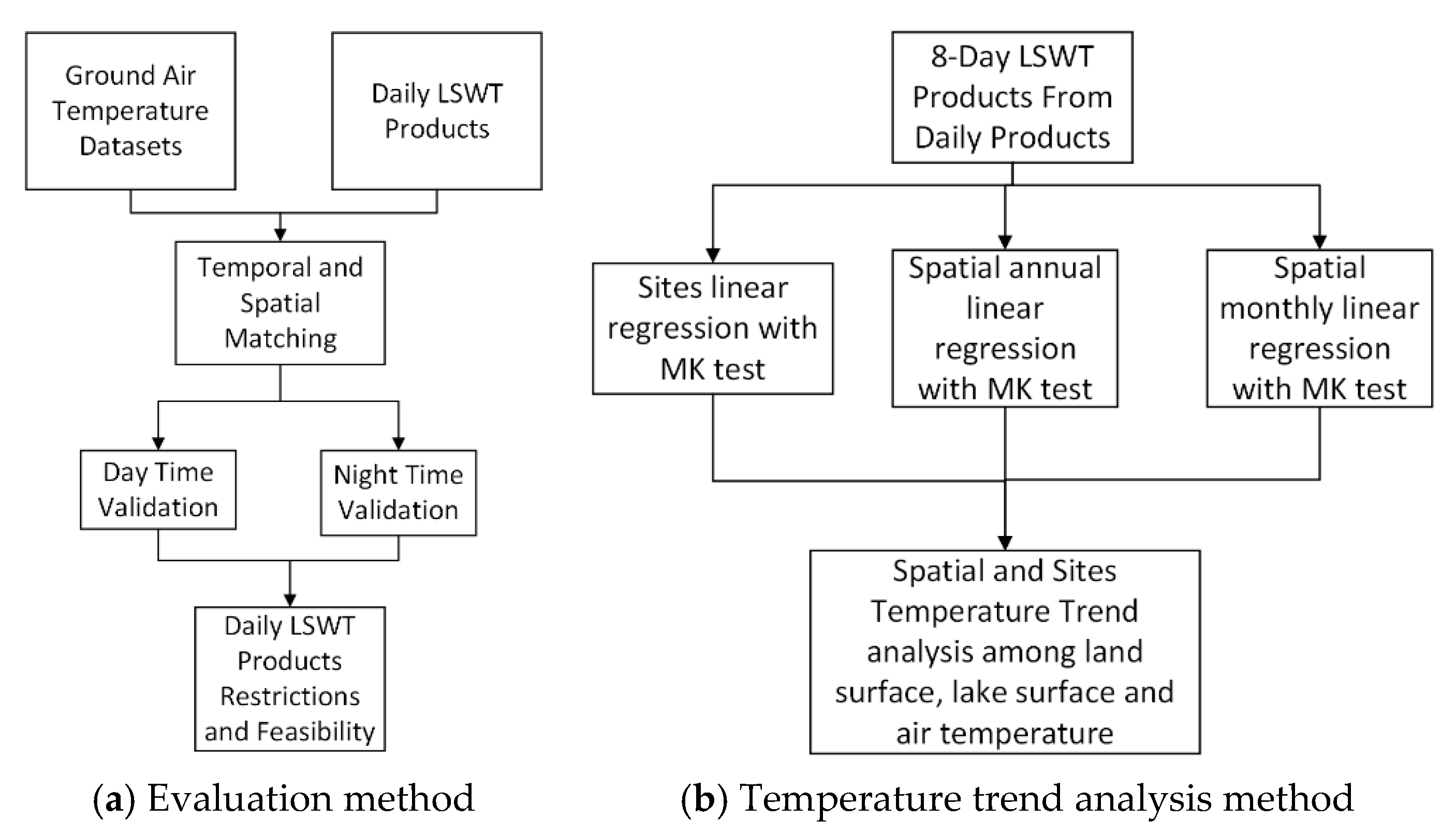
The ground temperature measurements from six sites, surrounding Kingston, managed by the Queen’s University Biological Station (QUBS), include air temperatures acquired at 15 min intervals from March to August in 2015–2017. However, not all sites have complete records due to the impacts of frozen ice in the winter and flowing waters in the spring melting season.

Table 1. Characteristics of the six QUBS sites for flooding seasons between 2015 and 2017.

Site Name	Longitude	Latitude	Land Cover *	Temporal Range			Code
				2015	2016	2017
Leroi Swamp	76.37° W	44.55° N	deciduous broadleaf	02.28–09.01	02.29–09.01	02.28–09.01	LS
Queen’s Point	76.32° W	44.56° N	woody savannas/water bodies	04.13–09.01	02.29–09.01	02.28–09.01	QP
Warner Lake	76.38° W	44.52° N	woody savannas	02.28–09.01	02.29–09.01	02.28–09.01	WL
Elbow Lake	76.42° W	44.47° N	water bodies	04.07–09.01	02.29–09.01	02.28–09.01	EL
Round Lake	76.40° W	44.54° N	deciduous broadleaf/woody savannas	02.28–09.01	02.29–09.01	02.28–09.01	RL
Hill Island	75.95° W	44.37° N	woody savannas	None	06.20–09.01	02.28–09.01	HI

*: The land cover was obtained from MCD12Q1—same source as Figure 1. Note that the land cover might not be consistent with Google Earth observations.

shows the major characteristics of the ground sites and the periods of each site with ground measurements each year. The accuracy of the ground-measured temperatures is +/−0.1 K at 283–303 K.

3. Methods

Figure 2 shows the scheme used in this paper. The evaluation part is important in remote sensing data applications, especially in climate analysis. Therefore, the daily LSWT products were first compared with ground air temperature measurements (Figure 2a). The daily LSWT products’ restrictions and feasibility could be obtained in this process. Based on the LSWT products’ performance analysis, the LSWT datasets were then used in the temperature trend analysis (Figure 2b). After that the site’s linear regression with an MK test was conducted and the results were analyzed.

3.1. Evaluation of MODIS Products with an In Situ Dataset

The evaluation using the flooding season datasets of QUBS air temperature was of Terra/MOD and Aqua/MYD LSWT products. It was accomplished for 2015–2017 (Figure 2a). The matchups were selected by the coincident and collocation areas between QUBS sites and MODIS pixels. The satellite datasets included Terra/MOD11A1 (Day/Night) and Aqua/MYD11A1 (Day/Night), at a spatial resolution of 1 km. The daytime and nighttime evaluations are accomplished separately to perform restriction and feasibility analysis of the LSWT products easily and clearly.

The total statistics and relationships between QUBS and MODIS were calculated, including the QUBS site’s mean, standard deviation (SD), centered root mean square difference (RMSD) and correlation. The statistics were all scaled according to the associated datasets. The mean and SD values are for MODIS and QUBS, separately. The RMSD and correlation were calculated between them.

For the LSWT datasets (T_si, i = 1 to n) and ground air temperature datasets (T_gi, i = 1 to n), the calculation methods are shown in the following equations:

$$\overline{{\mathrm{T}}_{\mathrm{g}}}=\frac{1}{\mathrm{n}}{\displaystyle \sum }_{\mathrm{i}=1}^{\mathrm{n}}{\mathrm{T}}_{\mathrm{gi}}$$

(1)

$$\overline{{\mathrm{T}}_{\mathrm{s}}}=\frac{1}{\mathrm{n}}{\displaystyle \sum }_{\mathrm{i}=1}^{\mathrm{n}}{\mathrm{T}}_{\mathrm{si}}$$

(2)

$${\mathrm{SD}}_{\mathrm{g}}=\sqrt{\frac{{{\displaystyle \sum }}^{ }{\left({\mathrm{T}}_{\mathrm{gi}}-\overline{{\mathrm{T}}_{\mathrm{g}}}\right)}^2}{\mathrm{n}}}$$

(3)

$${\mathrm{SD}}_{\mathrm{s}}=\sqrt{\frac{{{\displaystyle \sum }}^{ }{\left({\mathrm{T}}_{\mathrm{si}}-\overline{{\mathrm{T}}_{\mathrm{s}}}\right)}^2}{\mathrm{n}}}$$

(4)

$$\mathrm{RMSD}=\sqrt{\frac{{{\displaystyle \sum }}^{ }{\left(\left({\mathrm{T}}_{\mathrm{si}}-\overline{{\mathrm{T}}_{\mathrm{s}}}\right)-\left({\mathrm{T}}_{\mathrm{gi}}-\overline{{\mathrm{T}}_{\mathrm{g}}}\right)\right)}^2}{\mathrm{n}}}$$

(5)

$$\mathrm{Correlation}=\frac{{{\displaystyle \sum }}^{ }\left({\mathrm{T}}_{\mathrm{si}}-\overline{{\mathrm{T}}_{\mathrm{s}}}\right)\left({\mathrm{T}}_{\mathrm{gi}}-\overline{{\mathrm{T}}_{\mathrm{g}}}\right)}{\sqrt{{{\displaystyle \sum }}^{ }{\left({\mathrm{T}}_{\mathrm{si}}-\overline{{\mathrm{T}}_{\mathrm{s}}}\right)}^2{{\displaystyle \sum }}^{ }{\left({\mathrm{T}}_{\mathrm{gi}}-\overline{{\mathrm{T}}_{\mathrm{g}}}\right)}^2}}$$

(6)

3.2. Monthly Temperature Trends Analysis from the MODIS Product

The commonly used linear regression was performed in the temperature trend analysis of the study area using the following equation:

$$\mathrm{y}=\mathrm{a}+\mathrm{bx}$$

where y denotes the LSWT; x is the time in years; a is the intercept; b is the slope (K year^–1), i.e., the warming or cooling rate.

In the annual temperature analysis, the 8-day monthly MODIS, including MOD11A2 and MYD11A2 daytime and nighttime datasets, were first averaged. Then, the monthly average temperature trends for the study area were calculated with the linear regression method. One should note the uncertainty created by ice throughout December–April in the high latitude areas. The monthly analysis was intended to be a good complement to the annual analysis.

3.3. Mann–Kendall (MK) Test

Long-term trends of satellite-derived LST have been studied through a parametric statistical method, such as linear regression, in many studies [16]. However, the warming or cooling trend beginnings or hiatuses might not pass the significance test within linear regression. The widely used Mann–Kendall (MK) test was used in this study to observe the change trend and its significance [37,38,39]. As opposed to the linear regression method, the assumption of a normal distribution of the satellite-derived datasets is not a concern in the MK method [26]. The statistical s is first defined as follows:

$$\mathrm{s}={\displaystyle \sum }_{\mathrm{i}=2}^{\mathrm{n}}{\displaystyle \sum }_{\mathrm{j}=1}^{\mathrm{i}-1}\mathrm{sign}\left({\mathrm{x}}_{\mathrm{i}}-{\mathrm{x}}_{\mathrm{j}}\right)$$

(7)

where ${\mathrm{x}}_{\mathrm{i}}$ and ${\mathrm{x}}_{\mathrm{j}}$ are sequential values in a series. Then the trend Z could be defined as:

$$\mathrm{Z}=\{\begin{array}{r}\frac{(\mathrm{s}-1)}{\sqrt{\frac{\mathrm{n}(\mathrm{n}-1)(2\mathrm{n}+5)}{18}}}, \mathrm{s}>0\\ 0, \mathrm{s}=0\\ \frac{(\mathrm{s}+1)}{\sqrt{\frac{\mathrm{n}(\mathrm{n}-1)(2\mathrm{n}+5)}{18}}}, \mathrm{s}<0\end{array}$$

(8)

When Z > 0, the trend is ascending; when Z < 0, the trend is declining. When the absolute values of Z are larger than 1.28, 1.64 and 2.32, the respective data fell within 90%, 95% and 99% confidence intervals, respectively.

4. Results

4.1. Evaluation Results of MODIS Products with In Situ Datasets

Air temperatures from six sites were first compared with MODIS datasets from 2015 to 2017 (Figure 3). To simplify, only the daytime (Figure 3a) and nighttime (Figure 3b) comparisons from the MYD11A2 are displayed. It should be noted that only datasets from the flooding season were compared to avoid the mixed-up lake ice and melt pixels. For example, all sites’ first year datasets were from March 12 to 23 August 2015, except the missing HI (Table 1). The time interval in those datasets is about 1–4 days normally, as mentioned before, due to the cloud obscuring the satellite observations. For HI, we had all other datasets from 2016 to 2017. In late March and early April, due to the cold weather, some frozen surfaces had low temperatures below 273.15 K (0 degree). In these time periods, the differences between the MODIS LSWT and ground air temperature are larger than in the warmer periods. The differences between the two datasets are about 3–4 K. There are a lot of scatter points off the y = x diagonal line in Figure 3a compared to Figure 3b, which indicates that the daytime MODIS LSWT had a lower correlation with ground air temperature than the nighttime MODIS LSWT. However, the overall MODIS LSWT accuracy was relatively high relative to the ground air temperature. The detailed statistics can be found in

Table 2. MODIS LSWT statistics from different QUBS sites for flooding seasons of 2015–2017.

Product	Code	$\overline{{\mathbf{T}}_{\mathbf{g}}}$	SDg (K)	RMSD (K)	Correlation
MOD-day time	LS	291.85	9.44	3.07	0.95
	QP	295.08	5.47	2.31	0.91
	WL	292.11	8.42	3.17	0.93
	EL	291.30	7.11	3.47	0.88
	RL	291.15	8.97	2.84	0.95
	HI	296.69	3.86	1.88	0.88
MOD-nighttime	LS	284.34	8.03	3.21	0.92
	QP	288.92	5.74	2.20	0.93
	WL	286.70	6.53	2.54	0.93
	EL	286.19	6.56	3.55	0.86
	RL	285.75	7.62	2.51	0.95
	HI	291.94	5.66	1.88	0.95
MYD-day time	LS	292.53	7.68	4.41	0.82
	QP	294.43	7.03	3.60	0.87
	WL	293.08	6.52	2.92	0.90
	EL	293.72	6.73	3.56	0.85
	RL	294.73	7.22	3.80	0.85
	HI	297.10	4.26	1.92	0.90
MYD-nighttime	LS	286.09	6.58	1.48	0.97
	QP	286.85	5.11	2.15	0.92
	WL	283.95	6.67	2.07	0.95
	EL	284.37	6.56	2.25	0.94
	RL	283.86	6.09	2.16	0.94
	HI	289.64	4.73	0.73	0.99

.

Since we used the flooding season datasets in the comparison, it is reasonable that the mean temperatures were all above 280 K (Table 2). As shown from Figure 1, HI sits south of the other five sites; hence, it had the highest temperatures among all six sites during both daytime and nighttime.

As shown in Table 2 and Figure 3, the MODIS LSWTs agree well with in situ air temperature measurements. Aqua/MYD nighttime datasets are highly correlated with ground measurements with a correlation of over 0.90 for 2015–2017. Meanwhile, the Terra/MOD daytime results are better correlated with the ground measurements than the Terra/MOD nighttime results. For the different sites, the best results are from HI with a correlation of 0.98 for Aqua/MYD nighttime. The worst results are those for HI and EL with a correlation of 0.88 for Aqua/MYD daytime. The nighttime LSWTs matched better with the ground air temperatures than the daytime products. Hence, the nighttime LSWTs were used in the following trend analysis of Lake Ontario seasonal temperature. Nevertheless, the differences between Terra/MOD and Aqua/MYD should be paid more attention in future analyses.

4.2. Temperature Trends Found by Linear Regression at Six Ground Sites from MODIS Datasets

To examine the temperature trend and its confidence interval, the linear trends of annual average temperature at the six sites during different periods were examined from the 8-day MODIS-derived nighttime LST product.

Table 3. Linear trends (K year⁻¹) of MODIS LSWT over six sites.

Product	Code	Period (2001/2003–2018)			Period (2001/2003–2012)			Period (2012–2018)			Period (2001/2003–2010)			Period (2010–2018)
		Slope	Intercept	Z Value	Slope	Intercept	Z Value	Slope	Intercept	Z Value	Slope	Intercept	Z Value	Slope	Intercept	Z Value
MOD-night-time	LS	0.06	274.92	1.52	0.09	274.74	1.03	−0.05	276.54	0	0.02	275.07	0	−0.01	276.03	−0.10
	QP	0.05	277.34	0.08	0.14	276.97	0.07	−0.11	279.98	0	−0.03	277.67	−0.72	0.02	277.92	−0.10
	WL	0.07	275.83	1.82	0.14	275.53	1.58	−0.01	277.15	0.30	0.05	275.90	0.72	−0.01	277.14	0.10
	EL	0.07	275.13	1.44	0.18	274.63	1.99	−0.07	277.18	0	0.08	275.05	1.07	−0.07	277.17	−0.31
	RL	0.04	276.02	1.14	0.11	275.72	1.17	−0.04	277.36	0	0.06	275.94	0.18	−0.04	277.27	−0.10
	HI	0.06	277.64	1.52	0.09	277.57	1.17	0.09	277.29	0.60	−0.07	278.21	−0.18	0.04	278.08	0.52
MYD-night-time	LS	0.06	273.89	1.13	0.22	273.24	1.97	−0.00	274.64	0.30	0.13	273.55	1.11	−0.03	275.06	−0.31
	QP	0.07	275.72	0.86	0.08	275.72	0	0.01	276.65	0	−0.09	276.33	−0.62	0.11	275.25	0.73
	WL	0.07	274.96	1.04	0.18	274.55	1.97	0.14	273.90	0.30	0.11	274.82	1.11	0.02	275.56	0.10
	EL	0.05	273.85	1.22	0.24	273.04	2.50	−0.02	274.62	0	0.19	273.22	1.86	−0.13	276.04	−0.73
	RL	0.04	275.95	0.77	0.19	275.37	2.15	0.08	275.39	0.30	0.17	275.50	1.36	−0.03	276.84	0.10
	HI	0.06	276.72	0.95	0.15	276.72	0.89	−0.01	276.32	0	0.18	276.28	0.62	0.02	277.13	0.10

* The MOD datasets started from 2001, whereas the MYD datasets started from 2003, due to the different operational date of the sensors. ** The Z values larger than 1.64, for which the data passed the 95% confidence test, are colored red.

shows the slope and intercept of the linear trend during 2003–2018, 2003–2012, 2012–2018, 2003–2010 and 2010–2018, and the corresponding Z value for the MK test. The Z values larger than 1.64, for which the data provide a 95% confidence interval, are colored red. The linear trend shows warming for the MYD nighttime datasets, since the Z values of 4/6 sites are larger than 1.64 for 2003–2012. For MYD nighttime datasets at the QP and HI sites over 2003–2012, as seen in Figure 1, the surfaces of these two sites are fulfilled with lake water in the MODIS pixels, which means that the LSWT trend is not obvious, even during the apparent warming period of other sites and the whole area (Table 3).

The highest Z value of 2.50 is for the EL site during 2003–2012, which passed the 99% confidence test. This means that the warming trend of 0.25 K year⁻¹ for EL according to the MYD datasets is highly significant. This warming trend was also the largest found among all six sites. For the period of 2003–2010, the data at EL also passed the 95% confidence test with a warming trend of 0.19 K year⁻¹.

For the other time periods of MOD and MYD, no significant trends could be concluded. For the slope lower than zero (declining), the absolute value of Z is lower than 1.28, which means the data did not pass the MK test.

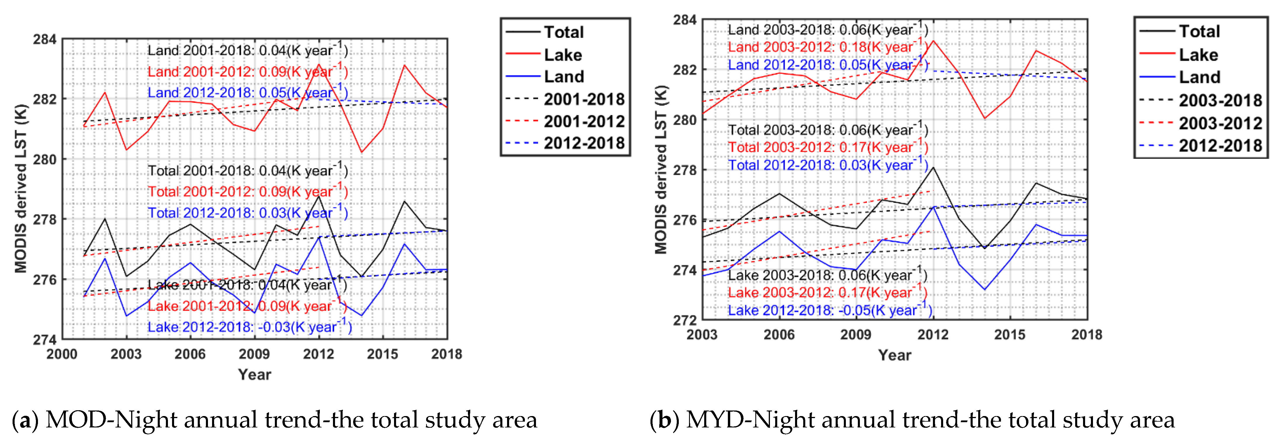
4.3. Spatial Patterns of Annual Temperature Trend Found by Linear Regression from MODIS Datasets

Further analysis was performed on the trend of total average temperature, with the data passing the 95% confidence threshold over the whole study region from MOD11A2 and MYD11A2 during 2001–2018 (Figure 4). The lake and land were differentiated using the HydroLAKES database (http://wp.geog.mcgill.ca/hydrolab/, accessed on 1 May 2021). MOD and MYD datasets showed similar trends for the total, lake and land regions. Generally, we found warming of 0.17 K year⁻¹ for MYD total during 2003–2012, and there was slight warming of 0.06 K year⁻¹ for the same datasets during 2003–2018. The MYD datasets show much clearer warming trends than the MOD datasets for both total and land regions. The MYD datasets for the lake region showed a warming trend both during 2003–2018 and during 2003–2012, and a slight cooling trend during 2012–2018.

The annual averaged temperature datasets from MOD11A2 and MYD11A2 for the period of 2001–2018 were then used to compute the annual spatial patterns of temperature trend via linear regression. The spatial temperature trends of regression slopes over the study area, with the data passing the 95% confidence threshold, are illustrated in Figure 5. The annual temperature trends from the nighttime MOD11A2 and MYD11A2 are shown for both periods, 2001/2003–2018 (Figure 5a,b) and 2001/2003–2012 (Figure 5A,B). The boxplots for both datasets are also shown for 2001/2003–2018 in Figure 5(a1,b1). Additionally, the annual temperature trends of the six ground sites, corresponding to the spatial distribution, are also listed in Figure 5(a2,b2).

The values that failed the 95% confidence threshold are shown in white in Figure 5. The MYD nighttime datasets for both periods show much more apparent warming trends over the study area than that the MOD nighttime ones. As in the site analysis in Section 4.2, the warming trend for MYD nighttime datasets is much more apparent over the whole study area, including Lake Ontario and its surroundings during 2003–2012. Some areas warmed by 0.25 K year⁻¹ according to MYD nighttime datasets (Figure 5B).

For the boxplot analysis, data within the 95% confidence threshold are shown in Figure 5(a1,b1). Apparently, no trend exists for the lake’s median value in either dataset over 2001/2003–2018. Meanwhile, a slight warming trend of around 0.1 K year⁻¹ is shown for the land’s median value.

The temperatures from the six ground sites’ annual trends show peaks in 2012 for both MOD (Figure 5(a2)) and MYD (Figure 5(b2)) datasets. As in the former results, during 2003–2012, the warming trends over the six ground sites were 0.18 K and 0.12 K year⁻¹ for MYD and MOD datasets, respectively. During the whole study period of 2001–2018, a warming trend of 0.06 K year⁻¹ was found by both datasets using the six ground sites.

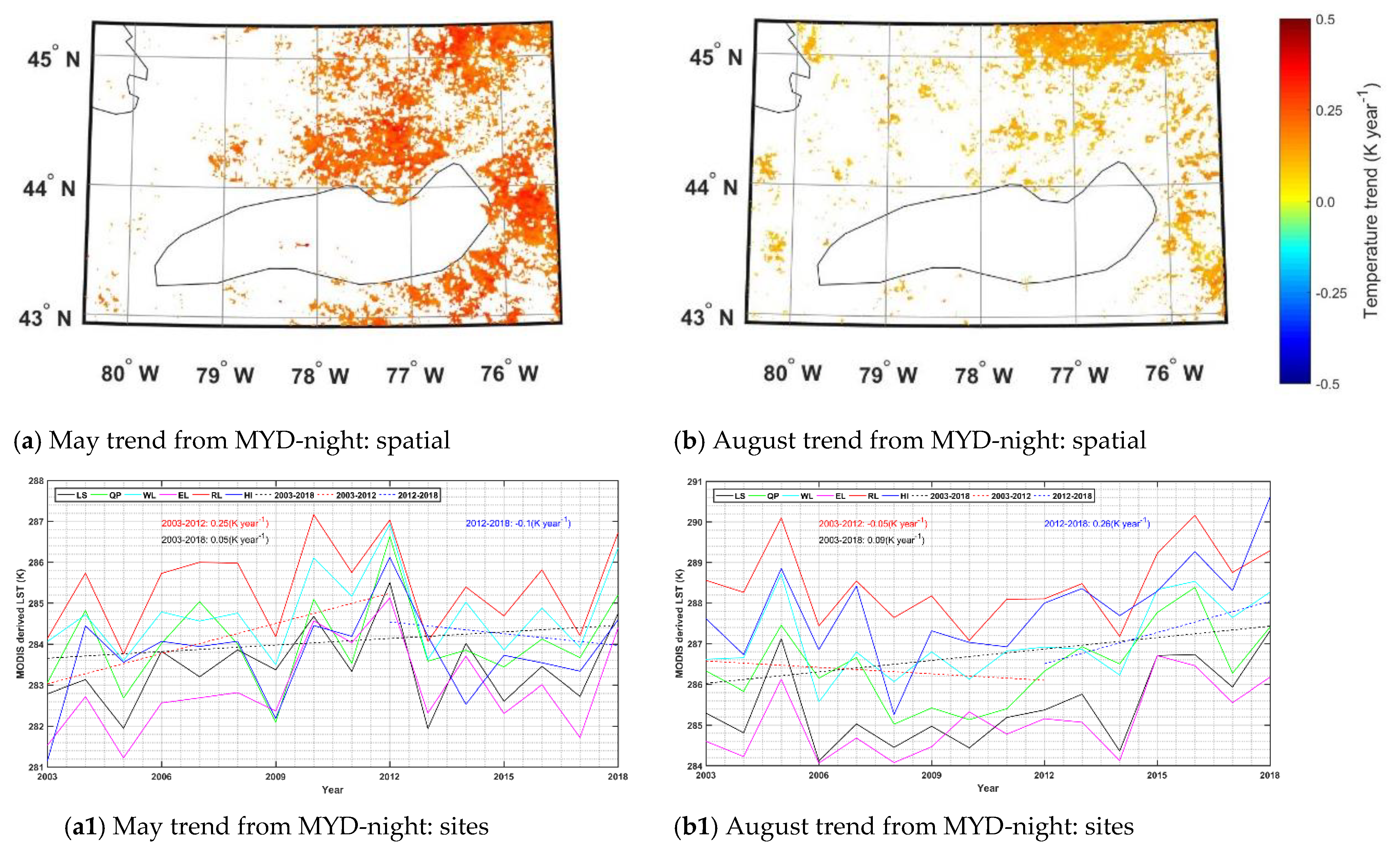
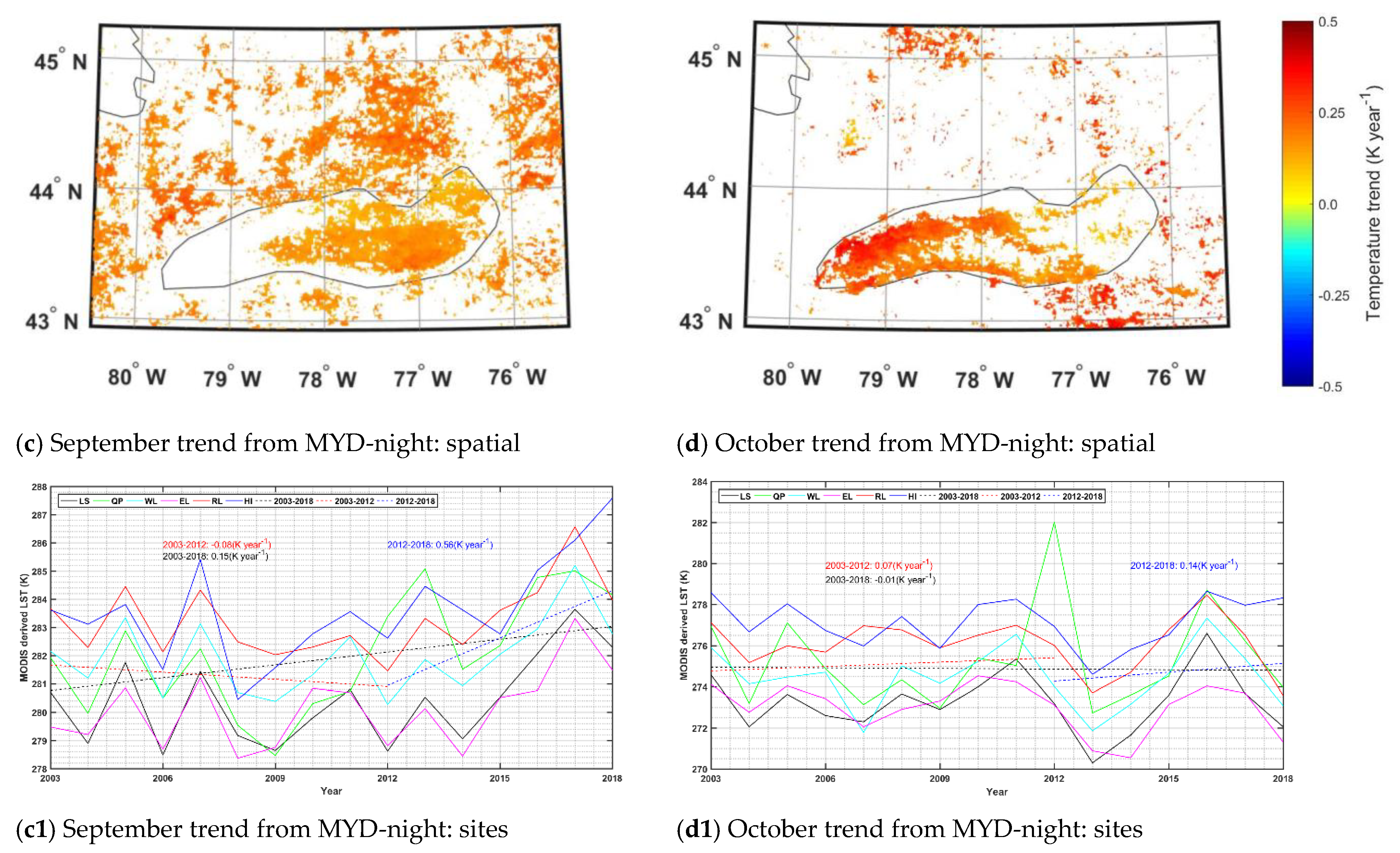
4.4. Spatial Patterns of Monthly Temperature Trend via Linear Regression from MODIS Datasets

For the monthly linear regression trends of the data within the 95% confidence interval, apparent warming trends over MYD datasets in May, August, September and October were selected and shown in Figure 6. The corresponding ground site trends are also shown.

The month of September (Figure 6c) had an apparent warming trend (mostly around 0.25 K year⁻¹) over the whole of Lake Ontario and its surroundings. Furthermore, the center of the lake showed the most obvious warming trend in September. For the months of May and August, no values were within the 95% confidence threshold for Lake Ontario itself, though a warming trend for the surroundings was found. On the contrary, the month of October showed an apparent warming trend over Lake Ontario, but no significant trend for its surroundings.

For the ground sites, an apparent warming trend of 0.56 K year⁻¹ was found for September during 2012−2018, and a declining trend of −0.08 K year⁻¹ was found for September during 2003−2012. The declining trends here are contradictory to the former results of annual trend analysis.

5. Discussion

5.1. The Relationship between LSWT and Air Temperature

The relationship between LST and air temperature have been widely discussed. The relationships between LSWT and air temperature in this study are shown in Figure 3 and Table 2. The air temperature measurements of EL and RL are of a lake, while the other four sites are situated on land. Therefore, both the relationships between LST/LSWT and air temperature are shown. However, there is not apparent difference between land and water surface temperatures in regard to air temperature. The RMSDs and correlations of EL and RL are not apparently better than those of the other four sites. Similarly to other studies of the relationships between LST and air temperature, the correlations of LSWT and air temperature are higher for nighttime temperatures than daytime temperatures.

5.2. The Similar Results from Other Lakes

Many similar analyses of LSWT, air temperature and their trends have been performed for both large and small lakes [40,41,42,43,44]. Some researchers focus on the Tibetan Plateau LSWT variations. Studies found that a global set of inland water bodies showed significant warming in seasonal nighttime LSWT between 1985 and 2009 [43].

Recently, many researchers conclude that the lakes in Tibetan Plateau partly show a warming trend [40,41], while others conclude a cooling trend [42]. The cooling trend in some way confirmed the global warming hiatus occurred during 1998 and 2012 [11,12].

5.3. The Possibilities for and Challenges of the MODIS Products in Lake Temperature Trend Analysis

In this part, pros and cons are summarized to illustrate the possibilities for and challenges of the MODIS-derived LSWT products in large lake temperature trend analysis:

Pro 1: Satellite observed thermal imagery has the advantage of providing a time-synchronized dense grid of temperature data at local, regional or even global scales [20,45]. MODIS-derived LSWT products could give the continuous spatial and temporal temperature record over the large lake, which the traditional field observations could not achieve, especially for remote and large lake areas. Moreover, MODIS and some other satellite products could be obtained from online ways relatively easier and cheaper than the acquisition of in situ datasets.

Pro 2: MODIS LSWT is relatively easily obtained, and the derived LSWT product has high accuracy for the lake surface according to the validation results in Section 3.1.

Pro 3: MODIS can not only provide LSWT products, but also some surface parameters which are of great importance for large lake analysis, such as ice phenology.

Con 1: MODIS has a short time series—less than 20 years. For climate change analysis, the time period is often over 30 years [9]. However, some researchers also claimed that the length of 17 years’ interval was required for identifying global warming trends [12]. This conclusion might give much more confidence in the satellite-derived temperature trend analysis.

Con 2: MODIS can only obtain records four times in a day. The clouds hinder the temporal acquisition greatly too. Even more, for small lakes, the LSWT is not highly correlated with the air temperature. However, some researchers have been making attempts at reconstructing daytime LST under cloud-covered conditions using MODIS land products and MSG geostationary satellite data [46].

Con 3: MODIS is unable to obtain a temperature depth profile of lake water.

The above are the major pros and cons for the MODIS datasets. Obviously, MODIS could give accurate spatial and temporal LSWT datasets over the large lake’s area. Although the duration may affect the trend analysis, the large number of spatial and temporal MODIS datasets could help the researchers to make up for the shortcomings when digging through the large amounts of information in satellite datasets. The combination of satellite observations, numerical simulations and ground measurements could allow much more accurate and consistent LSWT trend analysis of large lakes [16,22].

6. Conclusions

LSWT is of great importance in climate change studies, especially for large lakes. To evaluate the feasibility of MODIS LSWT products in warming trend analysis from satellite observations, this research first used in situ measurements collected by QUBS to compare them with satellite-derived daily LSWT. The results show that the satellite-derived LSWT correlated well with in situ air temperatures, especially at nighttime. We can clearly see that the air temperature is much closer to satellite LSWTs at nighttime due to the stable nighttime air conditions. The MODIS LSWTs still match well with in situ air temperatures of the daytime for the large lake’s surface and dense vegetation surface in this research. More detailed analysis, including comparing freezing times using satellite data and air temperatures, should be carried out before the warming trend analysis in the future.

The 8-day MODIS datasets were used in the temperature trend analysis over the duration of nearly twenty years of 2001–2018. For the six ground sites, detailed temperature analysis was accomplished using the MK test method. A slight warming trend with 95% confidence was concluded over the ground sites from 2003–2012 for MYD11A1 night datasets. The warming trend for the whole region, including both lake and land, was about 0.17 K year⁻¹ for MYD11A1 datasets during 2003–2012, and about 0.06 K year⁻¹ during 2003–2018.

The spatial annual trend also showed a slight warming trend from 2003–2012 for MYD11A1 night datasets. Compared with other months the monthly temperatures of September and October over the study area show slight warming trends from 2003 to 2018. However, Lake Ontario showed less warming than its surroundings. Overall, the warming trend is much clearer during 2003–2012 than during 2003–2018.

Overall, our analysis indicates that the MODIS LSWT datasets have a powerful potential for large lake spatial-temporal temperature trend analysis. In this research, we only used the MODIS temperature products for the trend analysis. The combination and integration of various temperature products from past archives and upcoming satellites could overcome the shortcomings of single sensors in climate change analysis and should be the future trend. The satellite datasets could give relative high accuracy of temperature change over the observed time period. However, the systematic and other inner differences between different sensors have uncertainties. MODIS-based LSWT products cannot totally replace in situ observations; however, they could overcome some limitations of field measurements, such as human error and environmental contaminations.

References

1. Adrian, R.; O’Reilly, C.M.; Zagarese, H.; Baines, S.B.; Hessen, D.O.; Keller, W.; Livingstone, D.M.; Sommaruga, R.; Straile, D.; Van Donk, E. Lakes as sentinels of climate change. Limnol. Oceanogr. 2009, 54, 2283–2297. [Google Scholar] [CrossRef] [PubMed]
2. Li, Z.L.; Tang, B.H.; Wu, H.; Ren, H.Z.; Yan, G.J.; Wan, Z.M.; Trigo, I.F.; Sobrino, J.A. Satellite-derived land surface temperature: Current status and perspectives. Remote Sens. Environ. 2013, 131, 14–37. [Google Scholar] [CrossRef] [Green Version]
3. Williamson, C.E.; Saros, J.E.; Vincent, W.F.; Smol, J.P. Lakes and reservoirs as sentinels, integrators, and regulators of climate change. Limnol. Oceanogr. 2009, 54, 2273–2282. [Google Scholar] [CrossRef]
4. Pivato, M.; Carniello, L.; Viero, D.P.; Soranzo, C.; Defina, A.; Silvestri, S. Remote sensing for optimal estimation of water temperature dynamics in shallow tidal environments. Remote Sens. 2020, 12, 51. [Google Scholar] [CrossRef] [Green Version]
5. Guo, L.; Zheng, H.; Wu, Y.; Zhang, T.; Zhang, B. Responses of Lake Ice Phenology to Climate Change at Tibetan Plateau. IEEE J. Sel. Top. Appl. Earth Obs. Remote Sens. 2020, 13, 3856–3861. [Google Scholar] [CrossRef]
6. Dörnhöfer, K.; Oppelt, N. Remote sensing for lake research and monitoring–Recent advances. Ecol. Indic. 2016, 64, 105–122. [Google Scholar] [CrossRef]
7. Good, E. Daily minimum and maximum surface air temperatures from geostationary satellite data. J. Geophys. Res. Atmos. 2015, 120, 2306–2324. [Google Scholar] [CrossRef]
8. Wan, Z. MODIS Land-Surface Temperature Algorithm Theoretical Basis Document (LST ATBD); Institute for Computational Earth System Science University of California: Santa Barbara, CA, USA, 1999. [Google Scholar]
9. Stocker, T.F.; Qin, D.; Plattner, G.-K.; Tignor, M.; Allen, S.K.; Boschung, J.; Nauels, A.; Xia, Y.; Bex, V.; Midgley, P.M. The Physical Science Basis. Contribution of Working Group I to the Fifth Assessment Report of the Intergovernmental Panel on Climate Change. 2013; Cambridge University Press: Cambridge, UK; New York, NY, USA, 2013; pp. 33–118. [Google Scholar]
10. Wang, X.; Xiao, J.; Li, X.; Cheng, G.; Ma, M.; Zhu, G.; Arain, M.A.; Black, T.A.; Jassal, R.S. No trends in spring and autumn phenology during the global warming hiatus. Nat. Commun. 2019, 10, 2389. [Google Scholar] [CrossRef]
11. Medhaug, I.; Stolpe, M.B.; Fischer, E.M.; Knutti, R. Reconciling controversies about the ‘global warming hiatus’. Nature 2017, 545, 41–47. [Google Scholar] [CrossRef]
12. Fyfe, J.C.; Meehl, G.A.; England, M.H.; Mann, M.E.; Santer, B.D.; Flato, G.M.; Hawkins, E.; Gillett, N.P.; Xie, S.-P.; Kosaka, Y. Making sense of the early-2000s warming slowdown. Nat. Clim. Chang. 2016, 6, 224–228. [Google Scholar] [CrossRef] [Green Version]
13. Fyfe, J.C.; Gillett, N.P.; Zwiers, F.W. Overestimated global warming over the past 20 years. Nat. Clim. Chang. 2013, 3, 767–769. [Google Scholar] [CrossRef]
14. An, W.; Hou, S.; Hu, Y.; Wu, S. Delayed warming hiatus over the Tibetan Plateau. Earth Space Sci. 2017, 4, 128–137. [Google Scholar] [CrossRef]
15. Li, L.; Zha, Y. Satellite-based regional warming hiatus in China and its implication. Sci. Total Environ. 2019, 648, 1394–1402. [Google Scholar] [CrossRef]
16. Ouyang, X.; Chen, D.; Feng, Y.; Lei, Y. Comparison of seasonal surface temperature trend, spatial variability, and elevation dependency from satellite-derived products and numerical simulations over the Tibetan Plateau from 2003 to 2011. Int. J. Remote Sens. 2019, 40, 1844–1857. [Google Scholar] [CrossRef]
17. Cheng, L.; Abraham, J.; Hausfather, Z.; Trenberth, K.E. How fast are the oceans warming? Science 2019, 363, 128–129. [Google Scholar] [CrossRef]
18. Parida, B.R.; Oinam, B.; Patel, N.R.; Sharma, N.; Kandwal, R.; Hazarika, M.K. Land surface temperature variation in relation to vegetation type using MODIS satellite data in Gujarat state of India. Int. J. Remote Sens. 2008, 29, 4219–4235. [Google Scholar] [CrossRef]
19. Jin, M.; Dickinson, R.E. Land surface skin temperature climatology: Benefitting from the strengths of satellite observations. Environ. Res. Lett. 2010, 5, 044004. [Google Scholar] [CrossRef] [Green Version]
20. Zhang, P.; Bounoua, L.; Imhoff, M.L.; Wolfe, R.E.; Thome, K. Comparison of MODIS Land Surface Temperature and Air Temperature over the Continental USA Meteorological Stations. Can. J. Remote Sens. 2014, 40, 110–122. [Google Scholar]
21. Mutiibwa, D.; Strachan, S.; Albright, T. Land Surface Temperature and Surface Air Temperature in Complex Terrain. IEEE J. Sel. Top. Appl. Earth Obs. Remote Sens. 2015, 8, 4762–4774. [Google Scholar] [CrossRef]
22. Ouyang, X.; Chen, D.; Lei, Y. A Generalized Evaluation Scheme for Comparing Temperature Products from Satellite Observations, Numerical Weather Model, and Ground Measurements Over the Tibetan Plateau. IEEE Trans. Geosci. Remote Sens. 2018, 56, 3876–3894. [Google Scholar] [CrossRef]
23. Botts, L.; Krushelnicki, B. The Great Lakes. An Environmental Atlas and Resource Book; ERIC: Washington, DC, USA, 1987. [Google Scholar]
24. Céleste Irambona, B.M. David Huard, Anne Frigon. In Lake Ontario Water Temperature in a Changing Climate; Report Presented to Ontario Power GEneration; Ouranos: Montreal, QC, Canada, 2017. [Google Scholar]
25. Nalley, D.; Adamowski, J.; Khalil, B.; Ozga-Zielinski, B. Trend detection in surface air temperature in Ontario and Quebec, Canada during 1967–2006 using the discrete wavelet transform. Atmos. Res. 2013, 132, 375–398. [Google Scholar] [CrossRef]
26. Mohsin, T.; Gough, W.A. Trend analysis of long-term temperature time series in the Greater Toronto Area (GTA). Theor. Appl. Climatol. 2010, 101, 311–327. [Google Scholar] [CrossRef]
27. Ghaderpour, E.; Vujadinovic, T.; Hassan, Q.K. Application of the least-squares wavelet software in hydrology: Athabasca River basin. J. Hydrol. Reg. Stud. 2021, 36, 100847. [Google Scholar] [CrossRef]
28. Masud, M.B.; Ferdous, J.; Faramarzi, M. Projected changes in hydrological variables in the agricultural region of Alberta, Canada. Water 2018, 10, 1810. [Google Scholar] [CrossRef] [Green Version]
29. Merritt, W.S.; Alila, Y.; Barton, M.; Taylor, B.; Cohen, S.; Neilsen, D. Hydrologic response to scenarios of climate change in sub watersheds of the Okanagan basin, British Columbia. J. Hydrol. 2006, 326, 79–108. [Google Scholar] [CrossRef]
30. Coll, C.; Caselles, V.; Galve, J.M.; Valor, E.; Niclos, R.; Sánchez, J.M.; Rivas, R. Ground measurements for the validation of land surface temperatures derived from AATSR and MODIS data. Remote Sens. Environ. 2005, 97, 288–300. [Google Scholar] [CrossRef]
31. Sohrabinia, M.; Rack, W.; Zawar-Reza, P. Analysis of MODIS LST compared with WRF model and in situ data over the Waimakariri River basin, Canterbury, New Zealand. Remote Sens. 2012, 4, 3501–3527. [Google Scholar] [CrossRef] [Green Version]
32. Ren, H.; Yan, G.; Chen, L.; Li, Z. Angular effect of MODIS emissivity products and its application to the split-window algorithm. ISPRS J. Photogramm. Remote Sens. 2011, 66, 498–507. [Google Scholar] [CrossRef]
33. Duan, S.-B.; Li, Z.-L.; Cheng, J.; Leng, P. Cross-satellite comparison of operational land surface temperature products derived from MODIS and ASTER data over bare soil surfaces. ISPRS J. Photogramm. Remote Sens. 2017, 126, 1–10. [Google Scholar] [CrossRef]
34. Duan, Z.; Bastiaanssen, W. A new empirical procedure for estimating intra-annual heat storage changes in lakes and reservoirs: Review and analysis of 22 lakes. Remote Sens. Environ. 2015, 156, 143–156. [Google Scholar] [CrossRef]
35. Lofgren, B.M.; Zhu, Y. Surface energy fluxes on the Great Lakes based on satellite-observed surface temperatures 1992 to 1995. J. Great Lakes Res. 2000, 26, 305–314. [Google Scholar] [CrossRef]
36. Cheng, J.; Cheng, X.; Meng, X.; Zhou, G. A Monte Carlo Emissivity Model for Wind-Roughened Sea Surface. Sensors 2019, 19, 2166. [Google Scholar] [CrossRef] [PubMed] [Green Version]
37. Chatterjee, S.; Bisai, D.; Khan, A. Detection of approximate potential trend turning points in temperature time series (1941–2010) for Asansol weather observation station, West Bengal, India. Atmos. Clim. Sci. 2013, 2014. [Google Scholar] [CrossRef] [Green Version]
38. Liu, Y.; Yue, T.; Jiao, Y.; Zhao, N.; Zhao, M. Temperature changes in the Heihe River Basin based on high accuracy surface modelling. Meteorol. Appl. 2019, 26, 720–732. [Google Scholar] [CrossRef]
39. Zhao, W.; He, J.; Yin, G.; Wen, F.; Wu, H. Spatiotemporal Variability in Land Surface Temperature Over the Mountainous Region Affected by the 2008 Wenchuan Earthquake From 2000 to 2017. J. Geophys. Res. Atmos. 2019, 124, 1975–1991. [Google Scholar] [CrossRef]
40. Zhang, G.Q.; Yao, T.D.; Xie, H.J.; Qin, J.; Ye, Q.H.; Dai, Y.F.; Guo, R.F. Estimating surface temperature changes of lakes in the Tibetan Plateau using MODIS LST data. J. Geophys. Res. Atmos. 2014, 119, 8552–8567. [Google Scholar] [CrossRef]
41. Wan, W.; Zhao, L.; Xie, H.; Liu, B.; Li, H.; Cui, Y.; Ma, Y.; Hong, Y. Lake surface water temperature change over the Tibetan plateau from 2001 to 2015: A sensitive indicator of the warming climate. Geophys. Res. Lett. 2018, 45, 11–177. [Google Scholar] [CrossRef]
42. Song, K.; Wang, M.; Du, J.; Yuan, Y.; Ma, J.; Wang, M.; Mu, G. Spatiotemporal variations of lake surface temperature across the Tibetan Plateau using MODIS LST product. Remote Sens. 2016, 8, 854. [Google Scholar] [CrossRef] [Green Version]
43. Hulley, G.C.; Hook, S.J.; Schneider, P. Optimized split-window coefficients for deriving surface temperatures from inland water bodies. Remote Sens. Environ. 2011, 115, 3758–3769. [Google Scholar] [CrossRef]
44. Toffolon, M.; Piccolroaz, S.; Majone, B.; Soja, A.M.; Peeters, F.; Schmid, M.; Wüest, A. Prediction of surface temperature in lakes with different morphology using air temperature. Limnol. Oceanogr. 2014, 59, 2185–2202. [Google Scholar] [CrossRef] [Green Version]
45. Jeppesen, E.; Beklioğlu, M.; Özkan, K.; Akyürek, Z. Salinization increase due to climate change will have substantial negative effects on inland waters: A call for multifaceted research at the local and global scale. Innovation 2020, 1. [Google Scholar] [CrossRef] [PubMed]
46. Zhao, W.; Duan, S.-B. Reconstruction of daytime land surface temperatures under cloud-covered conditions using integrated MODIS/Terra land products and MSG geostationary satellite data. Remote Sens. Environ. 2020, 247, 111931. [Google Scholar] [CrossRef]
Figure 1. The land cover map of the study area (a) and the positions of the six ground sites (b) indicated by the red rectangles, obtained in 2017. The land cover map was obtained from MODIS land cover product MCD12Q1, in which the International Geosphere-Biosphere Program (IGBP) global vegetation classification was chosen: 1. Evergreen Needleleaf 3. Deciduous Needleleaf 4. Deciduous Broadleaf 5. Mixed Forest 8. Woody Savannas 9. Savannas 10. Grasslands 11. Permanent Wetlands 12. Croplands 13. Urban and Built-up 14. Cropland Mosaics 16. Bare Soil and Rocks 17. Water Bodies. The satellite images of the six ground sites are downloaded from Google Earth. (ch) indicates the positions and land cover details of the six ground sites: (c) Elbow Lake, (d) Hill Island, (e) Leroi Swamp, (f) Queen’s Point, (g) Round Lake, (h) Warner Lake.
Land 10 01315 g001aLand 10 01315 g001b
Figure 2. The scheme in this study. (a) Evaluation method; (b) Temperature trend analysis method.
Land 10 01315 g002
Figure 3. Scatter plots for temperature between MYD11A2 products and QUBS datasets for flooding seasons (March to September) of 2015–2017: (a) daytime; (b) nighttime.
Land 10 01315 g003
Figure 4. Total study area’s annual trend (K year−1) from MOD11A2 (a) and MYD11A2 (b) nighttime LST for different time periods. The HydroLAKES database (http://wp.geog.mcgill.ca/hydrolab/, accessed on 1 May 2021) was used to differentiate lake and land. The dotted lines are the linear regression lines for different time periods including 2001/2003−2018, 2003−2012 and 2012−2018.
Land 10 01315 g004
Figure 5. Annual trends (K year−1) from MOD11A2 and MYD11A2 nighttime LSWT for the periods of 2001/2003−2018 (a,b) and 2001/2003−2012 (A,B). Boxplots (a1,b1): For each box, the central value indicates the median, and the lower and top edges of the box indicate the 25th and 75th percentiles, respectively. The whiskers extend to the most extreme data points not considered outliers, and the outliers are plotted individually using the “+” symbol. The HydroLAKES database (http://wp.geog.mcgill.ca/hydrolab/, accessed on 1 May 2021) was used to differentiate lake and land. The ground sites trend from MOD over 2001−2018 (a2) and MYD over 2003−2018 (b2). The dotted lines are the linear regression lines for different time periods, including 2001/2003−2018, 2003−2012 and 2012−2018.
Land 10 01315 g005
Figure 6. Monthly trend (K year−1) from MYD11A2 nighttime LSWT for the period of 2003−2018. May: (a) spatial, (a1) site. August: (b) spatial, (b1) site. September: (c) spatial, (c1) site. October: (d) spatial, (d1) site. The dotted lines are the linear regression lines for different time periods, including 2003−2018, 2003−2012 and 2012−2018.
Land 10 01315 g006aLand 10 01315 g006b