Article

Exploring Assembly Trajectories of Abandoned Grasslands in Response to 10 Years of Mowing in Sub-Mediterranean Context

by
Alessandro Bricca
1,
Federico Maria Tardella
2,*,
Arianna Ferrara
1,
Tiziana Panichella
3 and
Andrea Catorci
1
1
School of Biosciences and Veterinary Medicine, University of Camerino, 62032 Camerino, Italy
2
School of Biosciences and Veterinary Medicine, Herbarium Universitatis Camerinensis, University of Camerino, 62032 Camerino, Italy
3
School of Advanced Studies, University of Camerino, 62032 Camerino, Italy
*
Author to whom correspondence should be addressed.
Land 2021, 10(11), 1158; https://doi.org/10.3390/land10111158
Submission received: 11 October 2021 / Revised: 22 October 2021 / Accepted: 26 October 2021 / Published: 29 October 2021
(This article belongs to the Special Issue Grassland Restoration)

Abstract

:
Abandoned semi-natural grasslands are characterized by lower plant diversity as a consequence of tall grasses spreading. Mowing is a widely used restoration practice, but its effects to maintain the restored diversity over time is poorly investigated in sub-Mediterranean grasslands. Since 2010 in the central Apennines, we fenced a grassland, invaded by Brachypodium rupestre, which was mowed twice a year. Before the experiment started, we recorded species cover in 30 random sampling units (0.5 m × 0.5 m). The sampling was repeated every two years for a total of ten years. We used linear mixed-effect models to investigate the trajectory of functional diversity and community weighted mean for traits related to space occupation, resource exploitation, temporal niche exploitation, and Grime’s CSR strategies. The reduction of the weaker competitor exclusion exerted by B. rupestre affected the functional plant community. In the short term (4–6 years), this fostered space occupation strategies, decreasing convergence of clonal strategies and horizontal space occupation types. In the longer term (8–10 years), mowing filtered ruderal strategies, i.e., species with faster resource acquisition (lower leaf dry matter content, LDMC). LDMC and CSR strategies, initially convergent due to the dominance of B. rupestre, lowered convergence over time due to higher differentiation of strategies.

1. Introduction

Semi-natural grasslands are an essential part of the European cultural landscape, being hotspots of biodiversity resulting from centuries or millennia of land use [1]. Grassland biodiversity is endangered by different drivers mainly related to processes of intensification or abandonment [2,3], with the latter particularly relevant in Mediterranean mountains [2,4,5]. Here, after World War II, the cessation of traditional management practices led to the abandonment of large areas [6,7], which are left to spontaneous vegetation regrowth, such as the expansion of shrublands or forest ecosystems at large scales [5,6] and invasion of competitive tall grasses at community scales [8,9,10,11,12].
In the Italian peninsula, two perennial species of Brachypodium are fostered by land-use cessation: Brachypodium rupestre (Host) Roem. & Schult. in low mountains, and B. genuense (DC.) Roem. & Schult. over 1300–1400 m a.s.l., both having competitive and stress-tolerant strategies. The competitive success of these Brachypodium species is related to their high tiller density and branching frequency [13], as well as to their capacity for clonal growth and clonal integration strategy [14]. Their invasive behavior causes a change in community structure and species composition [8,10,15,16]. Overall, the increase of tall-grass species leads to a marked drop of species richness and species diversity [10,17,18], by a process called “weaker-competitor exclusion” [19]. This process suggests that the prevalence of hierarchical differences in the competitive ability between species should favor strong competitors which remove all those species with less competitive abilities [17,20], leading to a community characterized by few ecologically similar species. In addition, tall-grass invasion may influence the temporal niche partitioning of coexisting species by selecting a set of species able to cope with environmental conditions (community structure, litter deposition, soil feature modifications, etc.) determined by dominant plants [15]. Finally, Brachypodium species are also unpalatable, reducing the nutrient value of pastures [21], negatively affecting shepherding, and further enhancing mountain farming abandonment [15,22].
Generally, grazing and mowing are the main management practices for grasslands, but grazers tend to avoid feeding on Brachypodium species at all (cattle) or they feed on it only in conditions of high stocking rates (sheep). However, in the latter case, B. rupestre can harm animal welfare, promoting a sudden and marked increase of rumen keratinization [23,24,25], which leads to a lower absorption of nutrients. Instead, a suitable management practice is mowing, which widely proved to be an appropriate management type for ensuring the high conservation value of grasslands [26]. It consists of a non-selective disturbance that reduces aboveground phytomass, prevents litter accumulation, and increases species diversity [8,27]. Moreover, mowing reduces the more dominant species mitigating the weaker competitor exclusion [28] as it is more destructive to the taller species because a larger proportion of their phytomass is removed [17,29].
We are still far away from understanding the mechanism of community response to a mowing regime, and further research is needed. Firstly, the effect of mowing has been mainly investigated in terms of taxonomical diversity [8,17,27,30,31], overlooking the community functional response. Secondly, short temporal scales have been mainly considered, focusing therefore only on the impact of mowing on invaded grasslands but not on the ability of mowing to maintain the restored diversity over time [28,29]. Thirdly, those scarce functional long-term investigations come from grasslands experiencing different management histories and climatic conditions compared to Mediterranean ones [17,32]. This prevents generalization of functional response to mowing across different geographic and climatic regions [33], so that functional long-term investigations in a Mediterranean context are urgently needed. Indeed, semi-natural Mediterranean grasslands share a valuable floristic composition and diversity [11], which is coupled with increasing interest for high-quality foods. This has led in recent years to a new thrust towards the production of meat and cheese from semi-extensive farms [34]. Moreover, Mediterranean grasslands are encompassed in the EU Habitats Directive and are the subject of public funding for their preservation and restoration [35].
In consideration of the above, this research was set up to investigate the effect during ten years of twice-a-year recurrent mowing on different functional dimensions of a grassland invaded by B. rupestre in a permanent area placed in central Apennines within a sub-Mediterranean climatic context. As functional dimensions, we considered a large set of measured plant functional traits capturing different strategies (space occupation; resource exploitation; temporal niche exploitation) in addition to Grime’s plant strategies [36]. The Grime’s scheme [37,38,39] is based on CSR theory reviewed by Grime and Pierce [40], in which the three principal strategies (competitor, stress tolerant, and ruderal) represent viable combinations arising under conditions of competition, abiotic limitation to growth, or periodic biomass destruction, respectively. CSR analysis has allowed strategies to be determined for a wide range of vascular plant species from habitats worldwide [36], and many examples have been produced at the species level [41,42]. In contrast, an approach involving ‘community strategy’ has been highly overlooked (but see [43]) even if it could provide key insights into the variability of adaptations within plant communities.
Previous investigation [27,31] ascertained the effectiveness of twice-a-year mowing in the recovery of taxonomic diversity and coenological composition of a grassland community invaded by B. rupestre. Here, we investigated the functional trajectory of this plant community during 10 years since the start of this disturbance regime. Assuming that the decrease of B. rupestre would lead to an increase of species diversity as evidenced by previous studies [8,10,27,31], by reducing the dominance of this species, we hypothesized that the reduction of the weaker competitor exclusion exerted by B. rupestre as a result of mowing twice a year would affect the functional plant community. In the short term, this would foster space occupation strategies to maximize the exploitation of the newly available resources, increasing divergence of clonal strategies, plant height, and horizontal space occupation types. We hypothesized also that in the longer term, mowing would shape a highly adapted plant community, positively filtering ruderal strategies, i.e., species with higher specific leaf area and lower leaf dry matter content and faster resource acquisition (a disturbance avoidance strategy), and also species that allocate resources in belowground clonal organs, which would ensure tolerance to mowing. We expected that an initial high convergence of leaf traits and CSR strategies due to the dominance of B. rupestre would have paved the way to higher differentiation of strategies in the community and, thus, a lowered convergence over time.
As far as leaf and flowering phenology are concerned, B. rupestre-dominated communities are characterized by temporal niche differentiation, which ensures species coexistence [44,45]. We expected that the decrease of B. rupestre led to the re-occupation of the most favorable period for flowering and photosynthesizing, i.e., in early summer at the maximum of phytomass production [46], reducing functional diversity (i.e., increased convergence). Specifically, our questions were:
(I)
Does mowing foster in the short term the divergence of spatial niche occupation strategies?
(II)
Does mowing reduce in the long term the convergence of temporal niche occupation strategies?
(III)
Does mowing favor the divergence of CSR strategies, leading to more ruderal communities, and how does this change reflect on leaf traits?

2. Materials and Methods

2.1. Study Area

The study area is located in the central Apennines (337398.00 m E, 4757200.00 m N, UTM-WGS84), encompassing north-facing slopes on limestone bedrocks. The area ranges from 1000 to 1300 m a.s.l. The climate is sub-Mediterranean [47], characterized by winter cold stress and summer drought stress. Mean annual rainfall is 1100 mm and the average annual temperature is 10–11 °C. Soils are neutral–sub acidic and their depth ranges from 20 to 40 cm. Its texture is mainly characterized by sand (8–10%), silt (32–35%), and clay (50–60%). Skeleton ranges from 25 to 40%, whereas total nitrogen averages from 6 to 7 g Kg−1 [48].
Grasslands that are not invaded by Brachypodium rupestre refer to Brizo mediae-Brometum erecti brizetosum mediae Biondi, Allegrezza and Zuccarello 2005 association (Cytiso spinescentis-Bromion erecti Bonin 1978 alliance, Erysimo-Jurineetalia bocconei S. Brullo 1984 order, and Festuco hystricis-Ononidetea striatae Rivas-Mart. et al. 2002 class). Productivity ranges from 170 to 220 g∙m−2. Beech woods of the Fagetalia sylvaticae order constitute the actual potential vegetation.
The area has had a century-old history of grazing by sheep and cattle, mainly during the period between late spring and late autumn, but in the last decades the number of grazing animals strongly decreased. Besides grazing, mowing has been carried out during the period of early summer on semi-flat slopes [48].

2.2. Sampling Design

In 2010, we selected the following elements as stratifying criteria to reduce macro-environmental variables among sampling units: topography features (altitude, ranging from 1000 to 1300 m a.s.l.; aspect, from west–north–west to east–north–east; slope, 20° to 50°).
Using remote sensing images and the QGIS software, the areas matching the stratifying criteria were overlaid with a grid of 100 m × 100 m and we selected those cells with a homogeneous aspect, slope angle, and sward cover. Following these criteria, we chose two adjacent cells of 1 ha each, with altitude equal to 1220–1280 m a.s.l., aspect north–west-facing and slope angle of 25°. In order to avoid disturbances by domestic and wild animals the cells were fenced.
As management practice, we selected two mowing events a year as previous research found the highest vascular plant species richness when the grassland was mown twice a year and hay was removed [49]. Moreover, experimental research suggests the adequacy of summer mowing to avoid reallocation of nutrients to storage organs [50].
One of the two selected cells was mown twice a year (i.e., end of June, before B. rupestre flowering, and at the end of October) starting from 2010 until 2019. Aboveground phytomass was removed and the sward was cut 2 cm above soil level using a grass trimmer and the mown phytomass and litter were hand removed every mowing event (i.e., twice a year). The other adjacent cell was left unmown and used as a control. Inside the fenced cells, using a QGIS generator of random points, a 5 m x 5 m grid was overlaid, and 30 points present at the crosses of the grid were randomly selected in each cell. Points close to the fence (<5 m) were excluded to avoid edge effects. Considering the findings of previous studies on community assembly rules [51], we assumed that fine-scale spatial resolution (0.5 m × 0.5 m) offered the most appropriate scale of study to detect the effect of biotic interactions. The 30 selected points were the lower left-hand corner of 30 sampling units (0.5 m × 0.5 m) per cell. For each year of data collection (2010, 2012, 2014, 2016, 2018, and 2020), 30 new sampling units were randomly placed to avoid temporal autocorrelation. In the unmown area, data were collected in 2010, before the start of the experiment, and in 2020, i.e., ten years later.

2.3. Data Collection

Relevés were all carried out at the end of June, before mowing. In each sampling point, we recorded the cover of each vascular species (visually estimated in percentage scale).
To understand the functional trajectory of the plant community induced by mowing twice a year, we selected a core of plant traits capturing different functional dimensions: competition for light and space occupation (plant vegetative height, H; horizontal architecture, HA) [52,53]; resource exploitation (specific leaf area, SLA; leaf dry matter content, LDMC) [53] and regulation of leaf temperature and water-use efficiency during photosynthesis (leaf area, LA) [53]; temporal niche exploitation (flowering phenology, FP; leaf phenology, LP) [27,52]; clonal strategy (clonal position, CP; clonal spread, CS) (adapted from [54]). Moreover, leaf traits (LA, SLA, and LDMC) were also used to calculate plant CSR (competitive, stress tolerant, and ruderal) strategies [39], by integrating both leaf economics (typical of S and R strategy selection) and leaf size (typical of the C strategy) variation spectra in a three-way trade-off [36]. These selected traits are related to both competitive ability and response to mowing [52,53,54,55]. A description of each trait and their respective list of states and data sources are reported in Table 1.
Data on SLA, LA, LDMC, and H were drawn from field measurements at the end of June 2019 in the surrounding areas sharing similar topographic conditions, following the protocols described by Perez-Harguindeguy et al. [56], i.e., taking measurements from 10 fully expanded leaves without signs of damage of different individuals per species. In total, we measured 860 individuals of 86 species. Even if we did not consider intraspecific variation, the approach adopted, which considered a mean trait value fixed for each species, is more advantageous compared to the use of a regional or global trait database since they rarely provide climatic or habitat information on trait collection sites [57]. Since measuring these quantitative traits for all the species was not feasible, to perform the following statistical analyses we considered the species whose relative cumulative plot cover (in decreasing order of abundance) reached at least 80% of the total plot cover [58]. This choice relies on the assumption that the ecosystem functioning and services depend strongly on the dominant species (biomass-ratio hypothesis) [59]. These trait values were then log10-transformed before running the analysis [58].
On the contrary, other traits were categorized by means of fuzzy coding in which species show multiple states of a trait (e.g., flowering time, Table 1). The percentage value of a species (0–100%) for each state was estimated dividing 1 by the number of the states. For example, species that can flower in both spring and summer would have a score of 0.5 for spring flowering and 0.5 as summer flowering [60]. Furthermore, Grime CSR strategies, calculated with the StrateFy CSR classification tool [36], have been treated as a fuzzy coded trait in which the C-, S-, and R-scores are expressed as a percentage (0–100%). Categoric traits were obtained through databases for all the species: LEDA for flowering time, leaf phenology, horizontal architecture [61]; CLO-PLA for clonal position and clonal spread [54] and supplemented by observations in the Herbarium Universitatis Camerinensis (CAME).

2.4. Statistical Analysis

Preliminarily, we calculated the mean and standard error of the mean for the number of species, the total vegetation cover (sum of species cover values), and the B. rupestre absolute and relative cover, for each year.
Then, to investigate the functional trajectory of the plant community along the experimental trail, we computed the functional diversity (hereafter, FD) with Rao’s Quadratic Entropy [62]. We selected Rao’s Q because it is the most widely used index for functional investigation [62,63] and it expresses the expected dissimilarity between two individuals of a given species assemblage selected at random with replacement. We calculated the FD for each plant trait as follows:
FD = i , j S d i j p i p j
where S is the number of species, pi and pj are the proportions of i-th or j-th species in the sampling unit, and dij is the functional distance or dissimilarity between the i-th and j-th species ranging from 0 (trait value of species i and j is exactly the same) to 1 (when two individuals have completely different trait values). As a measure of distance (dij) we used the Gower distance [64], implemented by de Bello et al. [60], since this is the appropriate distance for functional analysis being able to handle fuzzy coded traits [60]. Since detecting assembly rules needs to compare the observed values with those expected by chance [65], we calculated for each FD a standardized effect size (SES), as (Iobs − Isim)/σsim, where Iobs is the observed value of FD, Isim is the mean of the expected FD, and σ is the standard deviation of expected FD. A distribution of SES values lower than 0 indicates functional convergence, while a distribution of SES above 0 indicates functional divergence, according to a two-tailed t-test [66]. Expected FD values were generated, shuffling 999 times trait values among the species in the entire data set (“between-plot randomization strategy”) [65]. This algorithm, assuming a null model in which each species may occur in each plot with any abundances, and in combination with Rao’s Quadratic Entropy, is sensitive to habitat filtering and limiting similarities, and is less affected by Type I error rates [65]. Since we did not expect any clear relationship (e.g., linear or non-linear) between response variables (i.e., SES-FD) and the predictor [67] (year), we used generalized additive mixed models (GAMMs; with a Gaussian distribution) to analyze the trajectory of the standardized effect size of functional diversity (SES-FD) for each plant trait in relation to the number of years of mowing (fixed effect). In the model, we set the knot parameter (k) to 4 to prevent overfitting. To account for the random distribution of the sampling units, we included as random intercept the identities of samples (each sample being composed of 30 sampling units, as one different random sample was taken every two years).
In order to have a better understanding of the meaning of FD variations, we computed the community weighted mean values (hereafter, CWM). This index is widely used to quantify the shifting in the functional strategy along environmental gradients and provides complementary information to FD [63]. We calculated CWMs as follows:
C W M = i = 1 S p i x i
where CWM is the community weighted mean value of a given plant trait (for quantitative traits) or relative contribution of each state (for categorical traits), S is the number of species, pi is the relative abundance of species I (i = 1,2, …, S), and xi is the trait value for species i. In the case of the CWMs, using observed values may lead to biased biological information due to the spurious correlation with the species composition matrix [68] resulting in higher inflated error Type I rates [69]. For this reason, we integrated generalized additive mixed models with the “Max Test” procedure which involved two independent permutation tests: one testing the species attributes–species composition link (“column-based permutation”) in which 999 times the species trait across species are shuffled randomly, and the other testing the plot attributes–species composition link (“row-based permutation”) in which 999 plot attributes are shuffled randomly across all plots [69]. A p-value for each permutation procedure (pi, row-based permutation; pc, column-based permutation) is estimated separately as the probability that the marginal adjusted R2 value of the observed model is significantly higher than a distribution of 999 expected marginal adjusted R2 values, according to a one-tailed t-test (α < 0.05). By picking the largest of the two p-values as results (pmax = max (pi, pc)), the type I error is controlled.
To exclude that the results that were related to factors unrelated to the treatment (e.g., climate variability), we performed a BACI (Before/After Control/Impact) analysis [70], where sampling is conducted at simultaneous time periods in treatment and control sites before and after treatment (2010 and 2020) [71]. We used mixed-effects models, modeling the two-level categorical variables Control/Impact (unmown vs. mown area) and Before (2010)/After (2020) treatment and their interaction term as fixed effects. A significant interaction term indicates a significant effect of the treatment. As sampling units were spatially nested in two locations and changed every year, we used the identities of samples (each sample being composed of 30 sampling units), as one different random sample was taken every year, before and after treatment nested inside the two sampled areas as random intercept. We ran the mixed-effects models for each of the SES-FD indices using the lme function of nlme R-package. Significance values were obtained using the Type II Wald Chi-square test and the Anova function (car R-package, version 2.1-5). For CWMs, we used the above mentioned approach (i.e., Max Test) (lme function, nlme R-package).
All statistical analyses were carried out using the R software, version 4.0.3 (R Foundation for Statistical Computing, Vienna, Austria, http://www.R-project.org). For the calculation of the FD index, we used the Rao function provided by de Bello et al. [58] and for the CWM, the functcomp function (FD package). To calculate Gower distance handling fuzzy coded traits, we used the gawsid function (gawdis package). To run the generalized additive mixed models, we used the gamm4 function (gamm4 package). In Tables S1 and S2 we reported the values of SES-FD and observed CWM calculated at plot level.

3. Results

In total, we found 138 species across all the years of the treatment in the mown area with mean values of 17 ± 0.54 (mean ± standard error mean) species per plot before the treatment, a peak after six years of 27 ± 0.59 and a slight decrease at the end of the experimental trial with 25 ± 0.79 species (Figure 1a). On the contrary, the total plot cover decreased linearly from 151 ± 5.6% at the beginning of the experiments to 113 ± 3.9% at the end of the manipulation (Figure 1b). Brachypodium rupestre cover decreased consistently for both absolute and relative cover (Figure 1c,d), with a proportional cover ranging from 34 ± 2.6% before the experiment to 4 ± 0.8% at the end of the experiment.

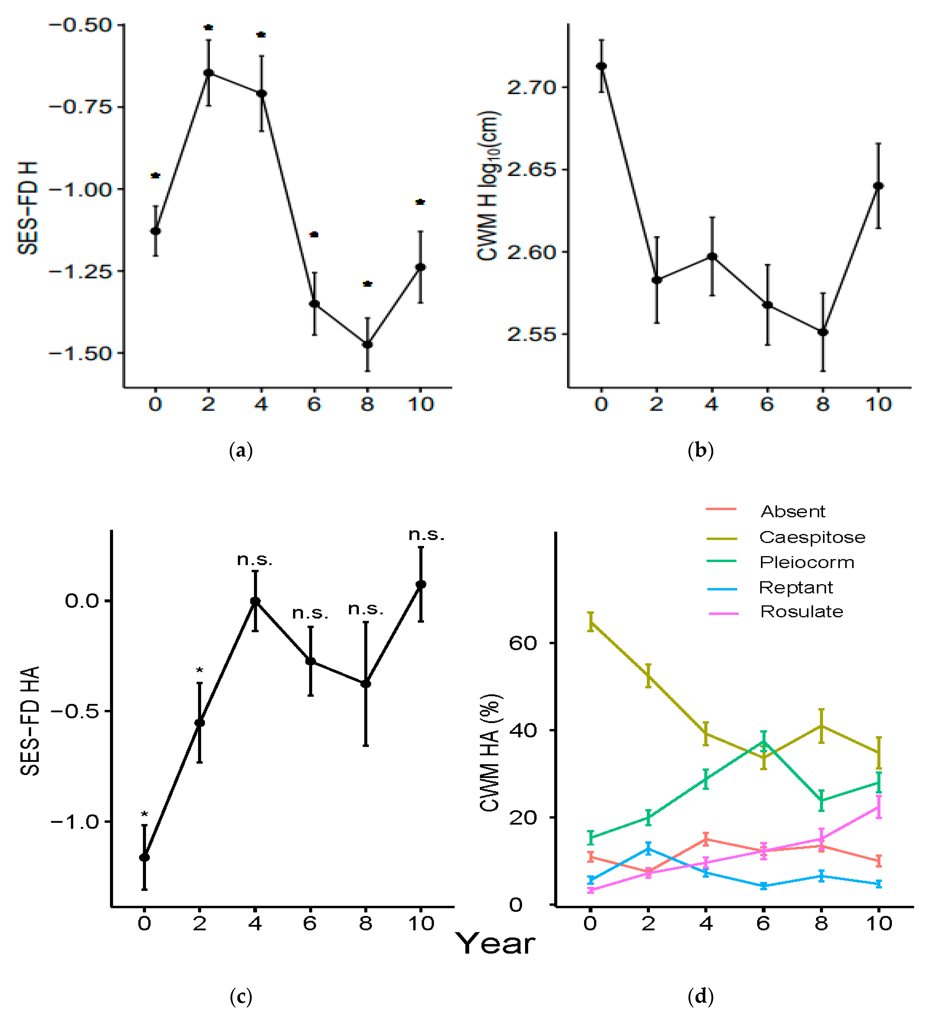
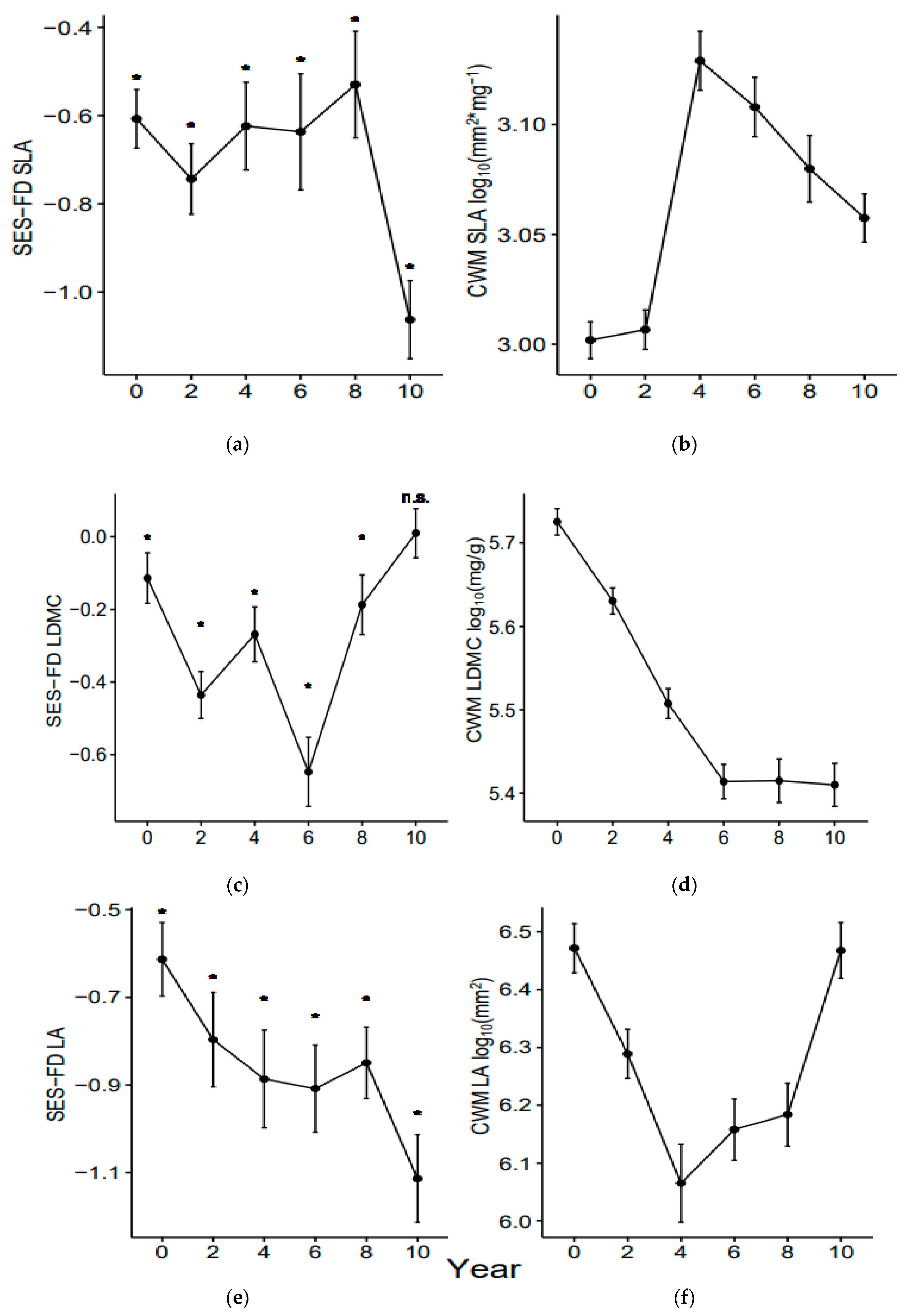
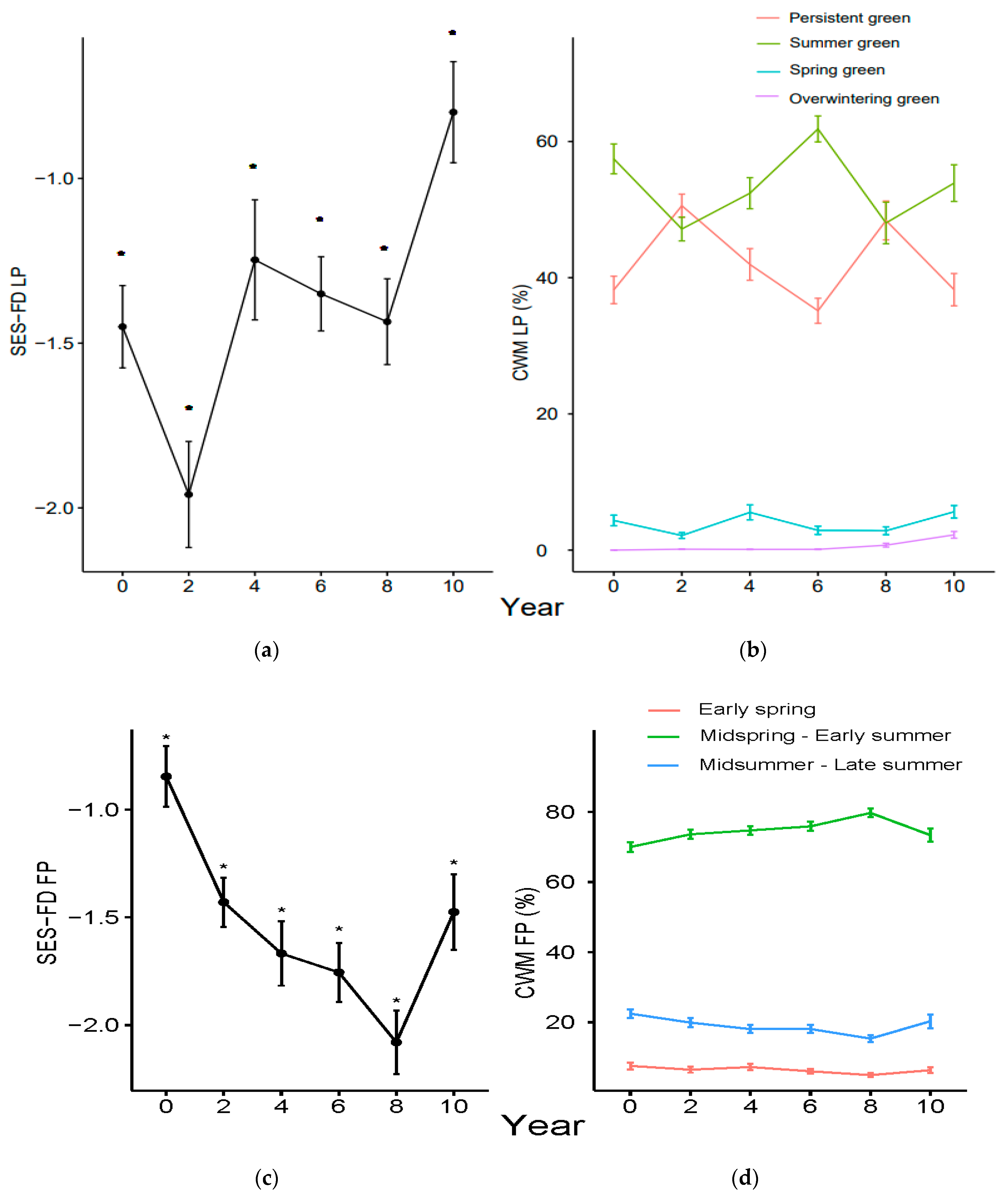
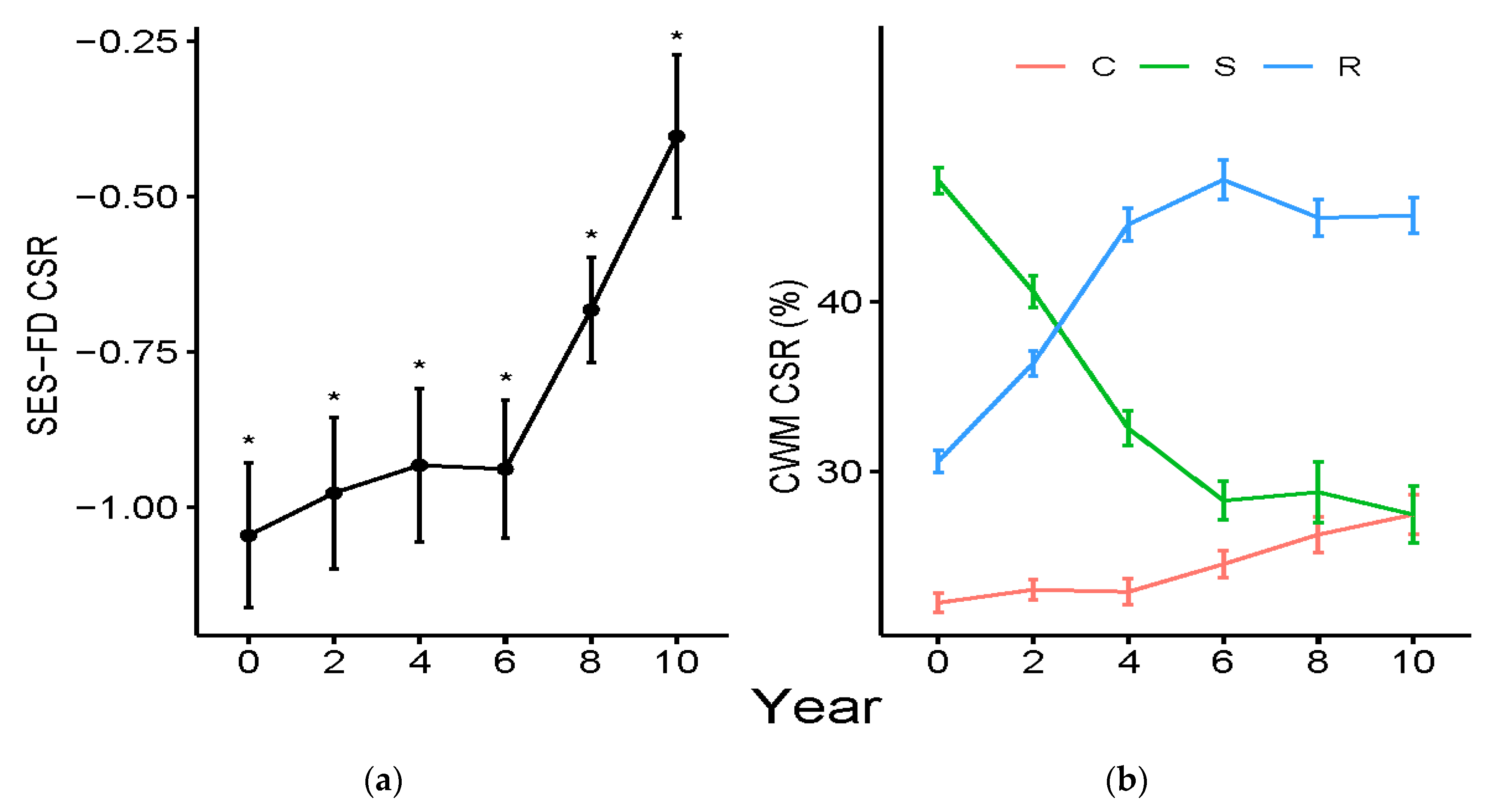
3.1. Functional Diversity Variation

Regarding the analysis of functional trajectories, we did not find any significant change, for the SES-FD of plant height (H), specific leaf area (SLA), leaf dry matter content (LDMC), leaf phenology (LP), and clonal spread (CS) (Table 2). Leaf area (LA), horizontal architecture (HA), flowering period (FP), and clonal propagation (CP) changed significantly during the experiment (Table 2). In detail, for space occupation (Figure 2), HA saw a cubic trend (edf = 2.6; Adj. R2 = 0.12, AIC = 522.0, Table 2, Figure 2c), whereas among the resource exploitation traits (Figure 3), those showing significant variation was LA (Figure 3e), with a linear relationship (edf = 1; Adj. R2 = 0.05, AIC = 292.9, Table 2). For the temporal niche exploitation (Figure 4) only FP showed significant changes, showing a quadratic relationship (edf = 2.2; Adj. R2 = 0.15, AIC = 438.94, Table 2, Figure 4a). For the clonal strategies only (Figure 5), CP showed a significant cubic relationship (edf = 2.6; Adj. R2 = 0.25, AIC = 457.23, Table 2, Figure 5a). Finally, also the Grime’s CSR strategies (Figure 6) showed significant changes in a quadratic trend (edf = 1.8; Adj. R2 = 0.01, AIC = 352.5, Table 2, Figure 6a). Detailed results for all plant traits (edf, Adj. R2, and model AIC values) are reported in Table 2. Finally, the analysis on the distribution of SES-FD pointed out mainly a functional convergence pattern for all traits across all years (SES-FD < 0). A shift from a convergence pattern to a random pattern occurred for HA and CP from 4 to 10 years (Figure 2c and Figure 5a), and in the last year of LDMC (Figure 3c). BACI analysis confirmed a significant effect of the treatment on SES-FD, for CP (Adj. R2 = 0.35; p < 0.05), HA (Adj. R2 = 0.58; p < 0.05), and Grime’s CSR strategy (Adj. R2 = 0.35; p < 0.05).

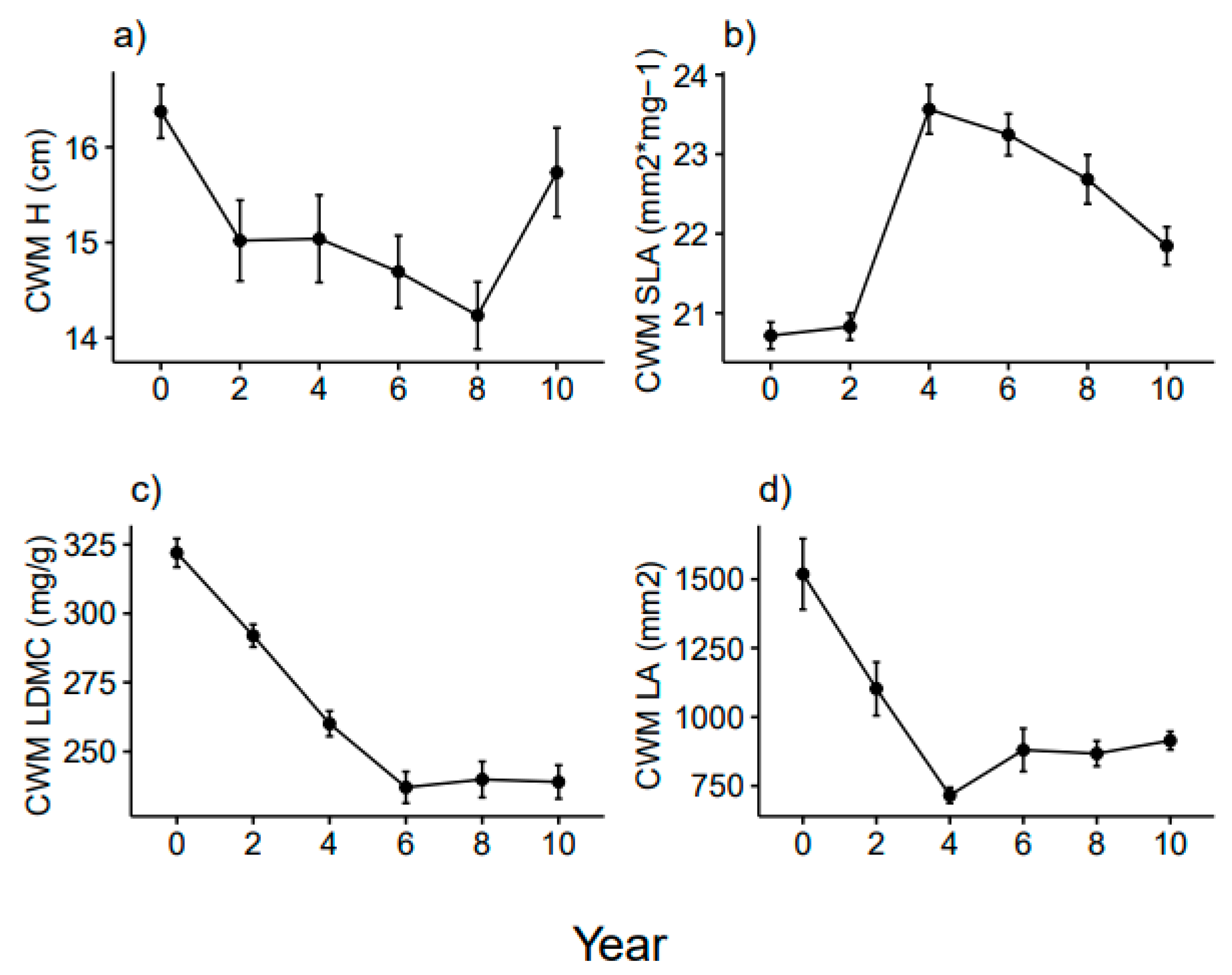
3.2. Community Weighted Mean Variation

Regarding the analysis of CWMs, all the results (i.e., edf, Adj. R2, and model AIC) are shown in Table 3. Significance was detected only for LDMC with a negative quadratic relationship (edf = 2.6; Adj. R2 = 0.53, AIC = −254.31, Table 3, Figure 3d). Moreover, for the Grime’s strategy, we found significant variation for S- and R-scores. For both S- and R-scores, we detected a negative and positive quadratic relationship, respectively (S-scores, edf= 2.6; Adj. R2 = 0.52, AIC = 1211.9, Table 3, Figure 6b; R-scores, edf = 2.6; Adj. R2 = 0.54, AIC =1114.8, Table 3, Figure 6b). BACI analysis confirmed a significant effect of treatment on LDMC (Adj. R2 = 0.63, pmax < 0.05), Grime’s stress-tolerant strategy (Adj. R2 = 0.68, pmax < 0.05), and ruderal strategy (Adj. R2 = 0.67, pmax < 0.05).
In Appendix A we report the graphs with non-log10-transformed CWM values of H, SLA, LA, and LDMC.

4. Discussion

The functional structure of the plant community was influenced differently by mowing over time (Figure 2, Figure 3, Figure 4, Figure 5 and Figure 6). In the first 4–6 years, mowing influenced the plant community probably through the weakening of the dominance of Brachypodium rupestre, highlighted by the decrease of its average cover value (Figure 1c,d) and by the fading of its weaker competitor exclusion effect, as suggested by the increase of species richness (Figure 1a). Contrariwise, after 6 years, the species richness value showed a fluctuation rather than a further increase (Figure 1a). In this second phase, the plant community was no longer dominated by B. rupestre, whose cover values tended to decrease to lower values (Figure 1c,d), and several SES-FD curves showed a variation in their trend (Figure 2a, Figure 3c, Figure 4c and Figure 5c). This variation in some cases was more marked in the last two years, giving rise to a clear inversion in the trend. This is consistent with Tardella et al. [27], who stated that the execution of mowing twice a year influences the functional structure of the plant community, leading to a condition strongly adapted to this type of disturbance.

4.1. Shorter-Term Variations

In the first phase of the experiment (up to 4–6 years), the plant community showed a variation of SES-FD for most of the considered traits. In particular, the decreasing deviations from the null model for plant height, horizontal space occupation, and leaf phenology types (i.e., decreasing convergence) seem to underline a rapid increase in the available spatial and temporal niches. Actually, the reduction of B. rupestre coverage likely exerted a positive effect on the appearance of gaps within the turf (spatial niche implementation) [10], while the aboveground phytomass and litter removal reduced the space occupied by the long-lasting (living or dead) leaves of the B. rupestre individuals, making available new temporal niches for exploitation of resources [52]. In particular, plant height was linked to competition for light, which is size-asymmetric, meaning that taller species (i.e., B. rupestre) can remove the shorter ones, leading to a plant community characterized by species functionally similar to the dominant ones [17] (Figure 2a,b). Our results underlined indeed a variation from a grassland characterized by a taller and less stratified canopy (year 0) to a grassland with a shorter canopy but characterized by more variable values, indicating probably a vertically stratified community (Figure 2a,b).
The invasion of B. rupestre forces the spring-flowering species in shelter niches where few individuals of each species remain [15], reducing the ecological spatial gaps necessary for species establishment [72,73]. The persistence of high amounts of aboveground phytomass of dominant species and of a litter layer fosters the coexistence of species that use different temporal niches for flowering [74,75]. The increase of convergence of flowering phenology (FP) soon after the beginning of phytomass and litter removal is consistent with this observation. We found indeed an increasing trend of mid-spring and early summer flowering species (Figure 4c). Such findings are in line with the “mid-domain hypothesis” [76], which suggests that a peak of flowering occurs when the site conditions are the most favorable.

4.2. Longer-Term Effects

In the second part of the experiment (4–6 to 8–10 years), the plant community showed different trends. Functional variation could be ascribed directly to the effect of mowing, with B. rupestre dramatically reduced (Figure 1c,d) and no longer able to exclude weaker competitors [17]. Interestingly, plant community adaptation to mowing seems to be driven mainly by specific traits. In this phase, indeed, some functional strategies such as HA and CP, whose SES-FD values were not significantly different from those expected by chance, seem to be driven by stochastic events (i.e., random assemblage) rather than by deterministic processes. Contrariwise, some traits linked to disturbance avoidance and tolerance strategies were largely affected [52,77]. In particular, the effect of mowing in shaping the plant community is well distinguished by the pattern of clonality. In fact, we observed a CWM increase for species having buried clonal organs and a decrease for species having above-soil clonal organs (Figure 5b). Belowground clonal organs (mostly epigeogenous rhizomes) may allow plants to minimize the loss of biomass. Such a trend is consistent with the results of investigations performed in the Mediterranean [52] and in the temperate climatic contexts [78], which asserted that short clonal organs are fundamental for plant resprouting (“tolerance mechanism”), as they allow a considerable storage of carbon [79]. Finally, the filtering effect of mowing is underlined by the more negative SES-FD values of plant height. Indeed, recurrent mowing tends to select a community characterized by species functionally similar in their size (i.e., short-sized species) (Figure 2a,b). This is consistent with the adaptation used by the plant to reduce the amount of aboveground phytomass removed [17,29].

4.3. Variation of Grime’s CSR Strategies

During the experimental trial we observed significant trends of the Grime’s strategies, with the decrease of stress-tolerant strategies and the increase of ruderal ones (Figure 6). This trend is in line with the general theory that disturbance repeated over time favors species with an overall ruderal strategy, i.e., species with avoidance and/or tolerance mechanisms [38,39]. Specifically, ruderal species do not invest a large proportion of resources in the individual growth but in propagules (i.e., seeds or clonal organs) by which the population can regenerate in case of disturbance [39]. Contrariwise, stress-tolerant species invest mainly in the capacity to retain resources, being present in resource-poor environments [38,39]. The higher CWM of stress tolerators at the beginning of the experimental trial results mainly in the higher proportion of B. rupestre, characterized mainly by a stress-tolerant performance (54%) in terms of resource exploitation and, secondly, by ruderal (26%) and competitive (20%) ones. The higher leaf plasticity allows it to spread in environments that experience different levels of stress intensity [80]. The combination of stress-tolerant resource exploitation strategies and tall stature has been seen as a functional portfolio for invasive species [81]. The increase in abundance of species having ruderal strategies is consistent with the pattern of leaf traits. Indeed, we observed the increase over time of species having lower LDCM values (Figure 3b,d,f), indicating a tendency toward fast-growth strategies [56].

5. Conclusions

The ongoing loss of biodiversity due to land-use variation is a worldwide concern that makes the recovery of abandoned grasslands a compelling issue. Since reintroducing the traditional land use in the sub-Mediterranean region is no longer economically sustainable for farmers, alternative practices should be found. In our study, we investigated the effect of recurrent mowing as an alternative practice to support the recovery of functional structure of abandoned grasslands. Overall, we found that the functional dimension of the studied plant community was influenced differently over time. In the first 4–6 years, mowing influenced indirectly the plant community, mostly through the weakening of the dominant ability of Brachypodium rupestre. This phase is characterized by the increase of species having fast-growing strategies. These species may suffer the competition with B. rupestre in abandoned grasslands, and also because they share the same flowering niche. In the second phase of the experiments (6–8 years), longer-term effects of mowing select directly the functional dimension of the plant community in that it tended to acquire functional adaptations based on avoidance strategies (e.g., lower LDMC) or tolerance strategies (e.g., belowground clonal organs). These trends are in line with Grime’s theory [39], as we observed that the plant community shifted towards ruderal strategies over time.
Finally, we have to note that concerning the latest years of the experimental trial we detected the start of a different trend for most of the considered traits. This is a hint that, after 10 years of recurrent mowing, the plant community might start to shift toward other different functional and ecological adaptations. This observation highlighted the importance of monitoring the plant community over the next years.

Supplementary Materials

The following are available online at https://www.mdpi.com/article/10.3390/land10111158/s1, Supplementary Table S1. Standardized effect size for functional diversity values (Rao’s Quadratic Entropy). Supplementary Table S2. Observed community weighted means of plant traits.

Author Contributions

Conceptualization, A.B. and A.C.; Data curation, A.B., F.M.T. and T.P.; Formal analysis, A.B. and A.F.; Investigation, F.M.T., T.P. and A.C.; Methodology, F.M.T.; Project administration, A.C.; Supervision, A.C.; Writing—original draft, A.B., A.F. and A.C.; Writing—review and editing, F.M.T. All authors have read and agreed to the published version of the manuscript.

Funding

This research received no external funding.

Data Availability Statement

The data presented in this study are available in supplementary material.

Acknowledgments

The authors wish to thank Mario Messini for the management of the fences.

Conflicts of Interest

The authors declare no conflict of interest.

Appendix A

Figure A1. Mean (±s.e.) of raw community weighted means (CWMs), i.e., non-log10-transformed, for (a) plant height (H), (b) specific leaf area (SLA), (c) leaf dry matter content (LDMC), and (d) leaf area (LA) under twice-a-year mowing. Year 0 (before treatment) refers to 2010; years 2, 4, 6, 8, and 10 correspond to 2012, 2014, 2016, 2018, and 2020.
Land 10 01158 g0a1

References

  1. Dengler, J.; Janišová, M.; Török, P.; Wellstein, C. Biodiversity of Palaearctic grasslands: A synthesis. Agric. Ecosyst. Environ. 2014, 182, 1–14. [Google Scholar] [CrossRef] [Green Version]
  2. Macdonald, D.; Crabtree, J.R.; Wiesinger, G.; Dax, T.; Stamou, N.; Fleury, P.; Lazpita, J.; Gibon, A. Agricultural abandonment in mountain areas of Europe: Environmental consequences and policy response. J. Environ. Manag. 2000, 59, 47–69. [Google Scholar] [CrossRef]
  3. Poptcheva, K.; Schwartze, P.; Vogel, A.; Kleinebecker, T.; Hölzel, N. Changes in wet meadow vegetation after 20 years of different management in a field experiment (North-West Germany). Agric. Ecosyst. Environ. 2009, 134, 108–114. [Google Scholar] [CrossRef]
  4. Catorci, A.; Foglia, M.; Tardella, F.M.; Vitanzi, A.; Sparvoli, D.; Gatti, R.; Galli, P.; Paradisi, L. Map of changes in landscape naturalness in the Fiastra and Salino catchment basins (central Italy). J. Maps 2012, 8, 97–106. [Google Scholar] [CrossRef] [Green Version]
  5. Ferrara, A.; Biró, M.; Malatesta, L.; Molnár, Z.; Mugnoz, S.; Tardella, F.M.; Catorci, A. Land-use modifications and ecological implications over the past 160 years in the central Apennine mountains. Landsc. Res. 2021, 1–13. [Google Scholar] [CrossRef]
  6. Bracchetti, L.; Carotenuto, L.; Catorci, A. Land-cover changes in a remote area of central Apennines (Italy) and management directions. Landsc. Urban Plan. 2012, 104, 157–170. [Google Scholar] [CrossRef]
  7. Malavasi, M.; Carranza, M.L.; Moravec, D.; Cutini, M. Reforestation dynamics after land abandonment: A trajectory analysis in Mediterranean mountain landscapes. Reg. Environ. Chang. 2018, 18, 2459–2469. [Google Scholar] [CrossRef]
  8. Bonanomi, G.; Caporaso, S.; Allegrezza, M. Short-term effects of nitrogen enrichment, litter removal and cutting on a Mediterranean grassland. Acta Oecol. 2006, 30, 419–425. [Google Scholar] [CrossRef]
  9. Catorci, A.; Ottaviani, G.; Cesaretti, S. Functional and coenological changes under different long-term management conditions in Apennine meadows (central Italy). Phytocoenologia 2011, 41, 45. [Google Scholar] [CrossRef]
  10. Catorci, A.; Cesaretti, S.; Gatti, R.; Ottaviani, G. Abiotic and biotic changes due to spread of Brachypodium genuense (DC.) Roem. & Schult. in sub-Mediterranean meadows. Community Ecol. 2011, 12, 117–125. [Google Scholar] [CrossRef]
  11. Giarrizzo, E.; Burrascano, S.; Chiti, T.; de Bello, F.; Lepš, J.; Zavattero, L.; Blasi, C. Re-visiting historical semi-natural grasslands in the Apennines to assess patterns of changes in species composition and functional traits. Appl. Veg. Sci. 2017, 20, 247–258. [Google Scholar] [CrossRef]
  12. Malatesta, L.; Tardella, F.M.; Tavoloni, M.; Postiglione, N.; Piermarteri, K.; Catorci, A. Land use change in the high mountain belts of the central Apennines led to marked changes of the grassland mosaic. Appl. Veg. Sci. 2019, 22, 243–255. [Google Scholar] [CrossRef]
  13. Pottier, J.; Evette, A. On the relationship between clonal traits and small-scale spatial patterns of three dominant grasses and its consequences on community diversity. Folia Geobot. 2010, 45, 59–75. [Google Scholar] [CrossRef]
  14. De Kroon, H.; Bobbink, R. Clonal plant dominance under elevated nitrogen deposition, with special reference to Brachypodium pinnatum in chalk grassland. In The Ecology and Evolution of Clonal Plants; De Kroon, G., Ed.; Backhuys Publishers: Kerkwerve, The Netherlands, 1997; pp. 359–379. [Google Scholar]
  15. Catorci, A.; Cesaretti, S.; Tardella, F.M. Effect of tall-grass invasion on the flowering-related functional pattern of submediterranean hay-meadows. Plant Biosyst. 2014, 148, 1127–1137. [Google Scholar] [CrossRef]
  16. Kılıç, D.D.; Kutbay, H.G.; Sürmen, B.; Hüseyinoğlu, R. The classification of some plants subjected to disturbance factors (grazing and cutting) based on ecological strategies in Turkey. Rend. Lincei Sci. Fis. Nat. 2018, 29, 87–102. [Google Scholar] [CrossRef]
  17. Lepš, J. Scale-and time-dependent effects of fertilization, mowing and dominant removal on a grassland community during a 15-year experiment. J. Appl. Ecol. 2014, 51, 978–987. [Google Scholar] [CrossRef]
  18. Filibeck, G.; Sperandii, M.G.; Bragazza, L.; Bricca, A.; Chelli, S.; Maccherini, S.; Wellstein, C.; Conte, A.L.; Di Donatantonio, M.; Forte, T.G.; et al. Competitive dominance mediates the effects of topography on plant richness in a mountain grassland. Basic Appl. Ecol. 2020, 48, 112–123. [Google Scholar] [CrossRef]
  19. Chesson, P. Mechanisms of maintenance of species diversity. Ann. Rev. Ecolog. Syst. 2000, 31, 343–366. [Google Scholar] [CrossRef] [Green Version]
  20. Mayfield, M.M.; Levine, J.M. Opposing effects of competitive exclusion on the phylogenetic structure of communities. Ecol. Lett. 2010, 13, 1085–1093. [Google Scholar] [CrossRef]
  21. Vitasović Kosić, I.; Tardella, F.M.; Grbeša, D.; Škvorc, Ž.; Catorci, A. Effects of abandonment on the functional composition and forage nutritive value of a North Adriatic dry grassland community (Ćićarija, Croatia). Appl. Ecol. Environ. Res. 2014, 12, 285–299. [Google Scholar] [CrossRef]
  22. Scocco, P.; Mercati, F.; Tardella, F.M.; Catorci, A. Increase of forage dryness induces differentiated anatomical response in the sheep rumen compartments. Microsc. Res. Tech. 2016, 79, 738–743. [Google Scholar] [CrossRef] [PubMed]
  23. Catorci, A.; Antolini, E.; Tardella, F.M.; Scocco, P. Assessment of interaction between sheep and poorly palatable grass: A key tool for grassland management and restoration. J. Plant Interact. 2014, 9, 112–121. [Google Scholar] [CrossRef]
  24. Scocco, P.; Brusaferro, A.; Catorci, A. Comparison between two different methods for evaluating rumen papillae measures related to different diets. Microsc. Res. Tech. 2012, 75, 884–889. [Google Scholar] [CrossRef] [PubMed]
  25. Scocco, P.; Mercati, F.; Brusaferro, A.; Ceccarelli, P.; Belardinelli, C.; Malfatti, A. Keratinization degree of rumen epithelium and body condition score in sheep grazing on Brachypodium rupestre. Vet. Ital. 2013, 49, 211–217. [Google Scholar] [CrossRef] [PubMed]
  26. Tälle, M.; Deák, B.; Poschlod, P.; Valkó, O.; Westerberg, L.; Milberg, P. Grazing vs. mowing: A meta-analysis of biodiversity benefits for grassland management. Agric. Ecosyst. Environ. 2016, 222, 200–212. [Google Scholar] [CrossRef]
  27. Tardella, F.M.; Bricca, A.; Goia, I.G.; Catorci, A. How mowing restores montane Mediterranean grasslands following cessation of traditional livestock grazing. Agric. Ecosyst. Environ. 2020, 295, 106880. [Google Scholar] [CrossRef]
  28. Halassy, M.; Botta-Dukát, Z.; Csecserits, A.; Szitár, K.; Török, K. Trait-based approach confirms the importance of propagule limitation and assembly rules in old-field restoration. Restor. Ecol. 2019, 27, 840–849. [Google Scholar] [CrossRef] [Green Version]
  29. Klimešová, J.; Janeček, Š.; Hornik, J.; Doležal, J. Effect of the method of assessing and weighting abundance on the interpretation of the relationship between plant clonal traits and meadow management. Preslia 2011, 83, 437–453. [Google Scholar]
  30. Milberg, P.; Tälle, M.; Fogelfors, H.; Westerberg, L. The biodiversity cost of reducing management intensity in species-rich grasslands: Mowing annually vs. every third year. Basic Appl. Ecol. 2017, 22, 61–74. [Google Scholar] [CrossRef] [Green Version]
  31. Tardella, F.M.; Malatesta, L.; Goia, I.G.; Catorci, A. Effects of long-term mowing on coenological composition and recovery routes of a Brachypodium rupestre-invaded community: Insight into the restoration of sub-Mediterranean productive grasslands. Rend. Lincei Sci. Fis. Nat. 2018, 29, 329–341. [Google Scholar] [CrossRef]
  32. Doležal, J.; Mašková, Z.; Lepš, J.; Steinbachová, D.; de Bello, F.; Klimešová, J.; Tackenberg, O.; Zemek, F.; Květ, J. Positive long-term effect of mulching on species and functional trait diversity in a nutrient-poor mountain meadow in Central Europe. Agric. Ecosyst. Environ. 2011, 145, 10–28. [Google Scholar] [CrossRef]
  33. Diaz, S.; Lavorel, S.; McIntyre, S.U.E.; Falczuk, V.; Casanoves, F.; Milchunas, D.G.; Skarpe, C.; Rusch, G.; Sternberg, M.; Noy-Meir, I.; et al. Plant trait responses to grazing–a global synthesis. Glob. Chang. Biol. 2007, 13, 313–341. [Google Scholar] [CrossRef]
  34. Martins, N.; Ferreira, I.C. Mountain food products: A broad spectrum of market potential to be exploited. Trends Food Sci. Technol. 2017, 67, 12–18. [Google Scholar] [CrossRef]
  35. Olmeda, C.; Keenleyside, C.; Tucker, G.; Underwood, E. Farming for Natura 2000 Guidance on How to Support Natura 2000 Farming Systems to Achieve Conservation Objectives, Based on Member States Good Practice Experiences; European Comission; Publications Office of the European Union: Luxembourg, 2014. [Google Scholar] [CrossRef]
  36. Pierce, S.; Negreiros, D.; Cerabolini, B.E.L.; Kattge, J.; Díaz, S.; Kleyer, M.; Shipley, B.; Wright, S.J.; Soudzilovskaia, N.A.; Onipchenko, V.G.; et al. A global method for calculating plant CSR ecological strategies applied across biomes world-wide. Funct. Ecol. 2017, 31, 444–457. [Google Scholar] [CrossRef]
  37. Grime, J.P. Vegetation classification by reference to strategies. Nature 1974, 250. [Google Scholar] [CrossRef]
  38. Grime, J.P. Evidence for the existence of three primary strategies in plants and its relevance to ecological and evolutionary theory. Am. Nat. 1977, 111, 1169–1194. [Google Scholar] [CrossRef]
  39. Grime, J.P. Plant Strategies, Vegetation Processes and Ecosystem Properties, 2nd ed.; Wiley: New York, NY, USA, 2001. [Google Scholar]
  40. Grime, J.P.; Pierce, S. The Evolutionary Strategies That Shape Ecosystems; Wiley-Blackwell: London, UK, 2012. [Google Scholar]
  41. Negreiros, D.; Le Stradic, S.; Fernandes, G.W.; Rennó, H.C. CSR analysis of plant functional types in highly diverse tropical grasslands of harsh environments. Plant Ecol. 2014, 215, 379–388. [Google Scholar] [CrossRef] [Green Version]
  42. Rosenfield, M.F.; Müller, S.C.; Overbeck, G.E. Short gradient, but distinct plant strategies: The CSR scheme applied to subtropical forests. J. Veg. Sci. 2019, 30, 984–993. [Google Scholar] [CrossRef]
  43. Zanzottera, M.; Dalle Fratte, M.; Caccianiga, M.; Pierce, S.; Cerabolini, B.E. Community-level variation in plant functional traits and ecological strategies shapes habitat structure along succession gradients in alpine environment. Community Ecol. 2020, 21, 55–65. [Google Scholar] [CrossRef]
  44. Catorci, A.; Ottaviani, G.; Vitasović Kosić, I.; Cesaretti, S. Effect of spatial and temporal patterns of stress and disturbance intensities in a sub-Mediterranean grassland. Plant Biosyst. 2012, 146, 352–367. [Google Scholar] [CrossRef]
  45. Corazza, M.; Tardella, F.M.; Ferrari, C.; Catorci, A. Tall grass invasion after grassland abandonment influences the availability of palatable plants for wild herbivores: Insight into the conservation of the Apennine chamois Rupicapra pyrenaicaornata. Environ. Manag. 2016, 57, 1247–1261. [Google Scholar] [CrossRef] [PubMed]
  46. Catorci, A.; Lulli, R.; Malatesta, L.; Tavoloni, M.; Tardella, F.M. How the interplay between management and interannual climatic variability influences the NDVI variation in a sub-Mediterranean pastoral system: Insight into sustainable grassland use under climate change. Agric. Ecosyst. Environ. 2021, 314, 107372. [Google Scholar] [CrossRef]
  47. Rivas-Martínez, S.; Sáenz, S.R.; Penas, A. Worldwide bioclimatic classification system. Glob. Geobot. 2011, 1, 1–634. [Google Scholar] [CrossRef]
  48. Catorci, A.; Cesaretti, S.; Gatti, R. Biodiversity conservation: Geosynphytosociology as a tool of analysis and modelling of grassland systems. Hacquetia 2009, 8, 129–146. [Google Scholar] [CrossRef] [Green Version]
  49. Socher, S.A.; Prati, D.; Boch, S.; Müller, J.; Baumbach, H.; Gockel, S.; Hemp, A.; Schöning, I.; Wells, K.; Buscot, F.; et al. Interacting effects of fertilization, mowing and grazing on plant species diversity of 1500 grasslands in Germany differ between regions. Basic Appl. Ecol. 2013, 14, 126–136. [Google Scholar] [CrossRef]
  50. Bobbink, R.; Den Dubbelden, K.; Willems, J.H. Seasonal dynamics of phytomass and nutrients in chalk grassland. Oikos 1989, 216–224. [Google Scholar] [CrossRef]
  51. Wellstein, C.; Campetella, G.; Spada, F.; Chelli, S.; Mucina, L.; Canullo, R.; Bartha, S. Context-dependent assembly rules and the role of dominating grasses in semi-natural abandoned sub-Mediterranean grasslands. Agric. Ecosyst. Environ. 2014, 182, 113–122. [Google Scholar] [CrossRef] [Green Version]
  52. Bricca, A.; Tardella, F.M.; Tolu, F.; Goia, I.; Ferrara, A.; Catorci, A. Disentangling the effects of disturbance from those of dominant tall grass features in driving the functional variation of restored grassland in a Sub-Mediterranean context. Diversity 2019, 12, 11. [Google Scholar] [CrossRef] [Green Version]
  53. Díaz, S.; Kattge, J.; Cornelissen, J.H.C.; Wright, I.; Lavorel, S.; Dray, S.; Reu, B.; Kleyer, M.; Wirth, C.; Prentice, I.C.; et al. The global spectrum of plant form and function. Nature 2016, 529, 167–171. [Google Scholar] [CrossRef]
  54. Klimešová, J.; De Bello, F. CLO-PLA: The database of clonal and bud bank traits of Central European flora. J. Veg. Sci. 2009, 20, 511–516. [Google Scholar] [CrossRef]
  55. Klimešová, J.; Latzel, V.; de Bello, F.; van Groenendael, J.M. Plant functional traits in studies of vegetation changes in response to grazing and mowing: Towards a use of more specific traits. Preslia 2008, 80, 245–253. [Google Scholar]
  56. Pérez-Harguindeguy, N.; Díaz, S.; Garnier, E.; Lavorel, S.; Poorter, H.; Jaureguiberry, P.; Bret-Harte, M.S.; Cornwell, W.K.; Craine, J.M.; Gurvich, D.E.; et al. Corrigendum to: New handbook for standardised measurement of plant functional traits worldwide. Aust. J. Bot. 2016, 64, 715–716. [Google Scholar] [CrossRef] [Green Version]
  57. Rosbakh, S.; Römermann, C.; Poschlod, P. Specific leaf area correlates with temperature: New evidence of trait variation at the population, species and community levels. Alp. Bot. 2015, 125, 79–86. [Google Scholar] [CrossRef]
  58. Májeková, M.; Paal, T.; Plowman, N.S.; Bryndová, M.; Kasari, L.; Norberg, A.; Weiss, M.; Bishop, T.R.; Luke, S.H.; Sam, K.; et al. Evaluating functional diversity: Missing trait data and the importance of species abundance structure and data transformation. PLoS ONE 2016, 11, e0149270. [Google Scholar] [CrossRef] [PubMed]
  59. Grime, J.P. Benefits of plant diversity to ecosystems: Immediate, filter and founder effects. J. Ecol. 1998, 86, 902–910. [Google Scholar] [CrossRef]
  60. de Bello, F.; Botta-Dukat, Z.; Lepš, J.; Fibich, P. Towards a more balanced combination of multiple traits when computing functional differences between species. Methods Ecol. Evol. 2021, 12, 443–448. [Google Scholar] [CrossRef]
  61. Kleyer, M.; Bekker, R.; Knevel, I.; Bakker, J.; Thompson, K.; Sonnenschein, M.; Poschlod, P.; van Groenendael, J.; Klimeš, L.; Klimešová, J.; et al. The LEDA Traitbase: A database of life-history traits of Northwest European flora. J. Ecol. 2008, 96, 1266–1274. [Google Scholar] [CrossRef]
  62. de Bello, F.; Lavergne, S.; Meynard, C.N.; Lepš, J.; Thuiller, W. The partitioning of diversity: Showing Theseus a way out of the labyrinth. J. Veg. Sci. 2010, 21, 992–1000. [Google Scholar] [CrossRef]
  63. Ricotta, C.; Moretti, M. CWM and Rao’s quadratic diversity: A unified framework for functional ecology. Oecologia 2011, 167, 181–188. [Google Scholar] [CrossRef]
  64. Pavoine, S.; Vallet, J.; Dufour, A.B.; Gachet, S.; Daniel, H. On the challenge of treating various types of variables: Application for improving the measurement of functional diversity. Oikos 2009, 118, 391–402. [Google Scholar] [CrossRef]
  65. Botta-Dukát, Z.; Czúcz, B. Testing the ability of functional diversity indices to detect trait convergence and divergence using individual-based simulation. Methods Ecol. Evol. 2016, 7, 114–126. [Google Scholar] [CrossRef]
  66. de Bello, F.; Šmilauer, P.; Diniz-Filho, J.A.F.; Carmona, C.P.; Lososová, Z.; Herben, T.; Götzenberger, L. Decoupling phylogenetic and functional diversity to reveal hidden signals in community assembly. Methods Ecol. Evol. 2017, 8, 1200–1211. [Google Scholar] [CrossRef]
  67. Wood, S.N. Generalized Additive Models: An Introduction with R; Chapman and Hall/CRC Press: Boca Raton, FL, USA, 2006. [Google Scholar]
  68. Zelený, D.; Schaffers, A.P. Too good to be true: Pitfalls of using mean E llenberg indicator values in vegetation analyses. J. Veg. Sci. 2012, 23, 419–431. [Google Scholar] [CrossRef]
  69. Zelený, D. Which results of the standard test for community-weighted mean approach are too optimistic? J. Veg. Sci. 2018, 29, 953–966. [Google Scholar] [CrossRef]
  70. Green, R.H. Sampling Design and Statistical Methods for Environmental Biologists; John Wiley & Sons: Hoboken, NJ, USA, 1979. [Google Scholar]
  71. Underwood, A.J. On beyond BACI: Sampling designs that might reliably detect environmental disturbances. Ecol. Appl. 1994, 4, 3–15. [Google Scholar] [CrossRef]
  72. Janeček, Š.; Lepš, J. Effect of litter, leaf cover and cover of basal internodes of the dominant species Molinia caerulea on seedling recruitment and established vegetation. Acta Oecol. 2005, 28, 141–147. [Google Scholar] [CrossRef]
  73. Jensen, K.; Gutekunst, K. Effects of litter on establishment of grassland plant species: The role of seed size and successional status. Basic Appl. Ecol. 2003, 4, 579–587. [Google Scholar] [CrossRef]
  74. Catorci, A.; Cesaretti, S.; Gatti, R.; Tardella, F.M. Trait-related flowering patterns in submediterranean mountain meadows. Plant Ecol. 2012, 213, 1315–1328. [Google Scholar] [CrossRef]
  75. Catorci, A.; Piermarteri, K.; Penksza, K.; Házi, J.; Tardella, F.M. Filtering effect of temporal niche fluctuation and amplitude of environmental variations on the trait-related flowering patterns: Lesson from sub-Mediterranean grasslands. Sci. Rep. 2017, 7, 1–14. [Google Scholar] [CrossRef] [PubMed] [Green Version]
  76. Morales, M.A.; Dodge, G.J.; Inouye, D.W. A phenological mid-domain effect in flowering diversity. Oecologia 2005, 142, 83–89. [Google Scholar] [CrossRef]
  77. Briske, D.D. Strategies of plant survival in grazed systems: A functional interpretation. In The Ecology and Management of Grazing Systems; Hodgson, I., Ed.; CAB International: Wallingford, UK, 1996; pp. 37–68. [Google Scholar]
  78. Klimeš, L.; Klimešová, J. The effects of mowing and fertilization on carbohydrate reserves and regrowth of grasses: Do they promote plant coexistence in species-rich meadows? In Ecology and Evolutionary Biology of Clonal Plants; Stuefer, J.F., Erschbamer, B., Huber, H., Suzuki, J.-I., Eds.; Springer: Dordrecht, The Netherlands, 2002; pp. 141–160. [Google Scholar]
  79. da Silveira Pontes, L.; Maire, V.; Schellberg, J.; Louault, F. Grass strategies and grassland community responses to environmental drivers: A review. Agron. Sustain. Dev. 2015, 35, 1297–1318. [Google Scholar] [CrossRef]
  80. Tardella, F.M.; Bricca, A.; Piermarteri, K.; Postiglione, N.; Catorci, A. Context-dependent variation of SLA and plant height of a dominant, invasive tall grass (Brachypodium genuense) in sub-Mediterranean grasslands. Flora 2017, 229, 116–123. [Google Scholar] [CrossRef]
  81. Conti, L.; Block, S.; Parepa, M.; Münkemüller, T.; Thuiller, W.; Acosta, A.T.; van Kleunen, M.; Dullinger, S.; Essl, F.; Dullinger, I.; et al. Functional trait differences and trait plasticity mediate biotic resistance to potential plant invaders. J. Ecol. 2018, 106, 1607–1620. [Google Scholar] [CrossRef] [Green Version]
Figure 1. Variation (mean ± s.e.) of (a) number of species, (b) total cover percentage, (c) Brachypodium rupestre absolute percentage cover, and (d) B. rupestre relative percentage cover during the treatment. Year 0 (before treatment) refers to 2010; years 2, 4, 6, 8, and 10 correspond to 2012, 2014, 2016, 2018, and 2020.
Land 10 01158 g001aLand 10 01158 g001b
Figure 2. Trends of standardized effect size of functional diversity (SES-FD) and community weighted means (CWMs) (mean ± s.e.) for (a,b) plant height (H) and (c,d) horizontal architecture (HA) under twice-a-year mowing. Year 0 (before treatment) refers to 2010; years 2, 4, 6, 8, and 10 correspond to 2012, 2014, 2016, 2018, and 2020. The asterisk (*) and n.s. indicate whether the distribution of SES-FD is significantly or not significantly different from zero after a one-sample two-tailed t-test (p < 0.05).
Land 10 01158 g002
Figure 3. Trends of standardized effect size of functional diversity (SES-FD) and community weighted means (CWMs) (mean ± s.e.) for (a,b) specific leaf area (SLA), (c,d) leaf dry matter content (LDMC), and (e,f) leaf area (LA) under twice-a-year mowing. Year 0 (before treatment) refers to 2010; years 2, 4, 6, 8, and 10 correspond to 2012, 2014, 2016, 2018, and 2020. The asterisk (*) and n.s. indicate whether the distribution of SES-FD is significantly or not significantly different from zero after a one-sample two-tailed t-test (p < 0.05).
Land 10 01158 g003
Figure 4. Trends of standardized effect size of functional diversity (SES-FD) and community weighted means (CWMs) (mean ± s.e.) for phenological traits; (a,b) leaf phenology (LP), (c,d) flower phenology (FP) under twice-a-year mowing. Year 0 (before treatment) refers to 2010; years 2, 4, 6, 8, and 10 correspond to 2012, 2014, 2016, 2018, and 2020. The asterisk (*) indicates a distribution of SES-FD significantly different from zero after a one-sample two-tailed t-test (p < 0.05).
Land 10 01158 g004
Figure 5. Trends of standardized effect size of functional diversity (SES-FD) and community weighted means (CWMs) (mean ± s.e.) for (a,b) clonal spread (CS), (c,d) clonal position (CP) under twice-a-year mowing. Year 0 (before treatment) refers to 2010; years 2, 4, 6, 8, and 10 correspond to 2012, 2014, 2016, 2018, and 2020. The asterisk (*) and n.s. indicate whether the distribution of SES-FD is significantly or not significantly different from zero after a one-sample two-tailed t-test (p < 0.05).
Land 10 01158 g005
Figure 6. Trends of standardized effect size of functional diversity (SES-FD); (a) and community weighted means (CWMs); (b) (mean ± s.e.) for Grimes’s CSR strategies under twice-a-year mowing. Year 0 (before treatment) refers to 2010; years 2, 4, 6, 8, and 10 correspond to 2012, 2014, 2016, 2018, and 2020. The asterisk (*) indicates a distribution of SES-FD significantly different from zero after a one-sample two-tailed t-test (p < 0.05).
Land 10 01158 g006
Table 1. List of the considered plant traits, variable type, and states of categorical traits.
Plant FunctionTraitVariable TypeTrait States
Competition for light and space occupancyPlant vegetative height (H)Continuous-
Horizontal architecture (HA)CategoricalAbsent, caespitose, pleiocorm, reptant, rosulate
Resource exploitationSpecific leaf area (SLA)Continuous-
Leaf dry matter content (LDMC)Continuous-
Water-use strategyLeaf area (LA)Continuous-
ReproductionFlowering period (FP)CategoricalEarly and mid-spring (March–April); late spring–early summer (May–June); mid-summer–early autumn (July–September)
Temporal resource exploitationLeaf phenology (LP)CategoricalOverwintering green, persistent green, spring green, summer green
PersistenceClonal position (CP)CategoricalAbove-soil, below-soil
Space occupancyClonal spread (CS)CategoricalAbsent, short-spread, long-spread
Table 2. Trends of standardized effect size of functional diversity under twice-a-year mowing of plant height (H), horizontal architecture (HA), specific leaf area (SLA), leaf dry matter content (LDMC), leaf area (LA), leaf phenology (LP), flower phenology (FP), clonal spread (CS), clonal position (CP), and Grime’s CSR strategies. Significant relations (p-value < 0.05) are indicated in bold. AIC values are referred to REML (restricted maximum likelihood). Effective degrees of freedom (edf) are a measure of the shape of the curves (with 1 completely linear; 2 completely quadratic; 3 completely cubic).
Traitedf Adj. R2AIC
H1 0.08299.6
HA2.60.12522.0
SLA2.3 0.06307.13
LDMC1.90.12214.8
LA10.05292.88
LP10.07442.0
FP2.20.15438.9
CS20.05400.2
CP2.60.25457.2
CSR Grime1.80.10352.5
Table 3. Trends of community weighted means under twice-a-year mowing for plant height (H), horizontal architecture (HA), specific leaf area (SLA), leaf dry matter content (LDMC), leaf area (LA), leaf phenology (LP), flowering phenology (FP), clonal spread (CS), clonal position (CP), and Grime’s CSR plant strategy. Significant relations (p-value < 0.05) are indicated in bold. AIC values are referred to REML (restricted maximum likelihood). Effective degrees of freedom (edf) are a measure of the shape of the curves (with 1 completely linear; 2 completely quadratic; 3 completely cubic).
TraitTrait StateedfAdj. R2AIC
H 2.30.13−180.3
HAAbsent1.0<0.01−470.2
Caespitose2.30.30−128.4
Pleiocorm1.80.18−252.8
Reptant1.00.04−511.3
Rosulate1.40.29−327.3
SLA 2.00.25−452.9
LDMC 2.60.53−254.3
LA 2.70.2373.6
LPPersistent green1.0<0.01−226.0
Summer green1.0<0.01−205.8
Spring green1.0<0.01−606.7
Overwintering green2.70.27−1032.9
FPEarly spring1.00.02−596.1
Mid-spring–Early summer1.90.10−397.6
Mid-summer–Late summer2.10.05−409.0
CSAbsent1.30.13−385.5
Short1.70.05−279.3
Long1.20.16−332.4
CPAbove1.00.24−381.1
Below2.20.11−318.0
CSRC1.30.131060.8
S2.60.521211.9
R2.60.541114.8
Publisher’s Note: MDPI stays neutral with regard to jurisdictional claims in published maps and institutional affiliations.

