
Quantification of Resilience Considering Different Migration Biographies: A Case Study of Pune, India


1
Department of Economic Geography and Location Research, Philipps-Universität Marburg, 30537 Marburg, Germany
2
UFZ—Helmholtz Centre for Environmental Research, Department of Economics, 04318 Leipzig, Germany
3
UFZ—Helmholtz Centre for Environmental Research, Department of Urban and Environmental Sociology, 04318 Leipzig, Germany
*
Author to whom correspondence should be addressed.
Land 2021, 10(11), 1134; https://doi.org/10.3390/land10111134
Submission received: 30 September 2021
/
Revised: 22 October 2021
/
Accepted: 22 October 2021
/
Published: 25 October 2021
(This article belongs to the Special Issue Urban-Rural-Partnerships: Sustainable and Resilient)
Abstract
:Urbanization proceeds globally and is often driven by migration. Simultaneously, cities face severe exposure to environmental hazards such as floods and heatwaves posing threats to millions of urban households. Consequently, fostering urban households’ resilience is imperative, yet often impeded by the lack of its accurate assessment. We developed a structural equation model to quantify households’ resilience, considering their assets, housing, and health properties. Based on a household survey (n = 1872), we calculate the resilience of households in Pune, India with and without migration biography and compare different sub-groups. We further analyze how households are exposed to and affected by floods and heatwaves. Our results show that not migration as such but the type of migration, particularly, the residence zone at the migration destination (formal urban or slum) and migration origin (urban or rural) provide insights into households’ resilience and affectedness by extreme weather events. While on average, migrants in our study have higher resilience than non-migrants, the sub-group of rural migrants living in slums score significantly lower than the respective non-migrant cohort. Further characteristics of the migration biography such as migration distance, time since arrival at the destination, and the reasons for migration contribute to households’ resilience. Consequently, the opposing generalized notions in literature of migrants either as the least resilient group or as high performers, need to be overcome as our study shows that within one city, migrants are found both at the top and the bottom of the resilience range. Thus, we recommend that policymakers include migrants’ biographies when assessing their resilience and when designing resilience improvement interventions to help the least resilient migrant groups more effectively.
1. Introduction
The megatrend of urbanization has largely become a phenomenon of the Global South [1]. The growth of urban centers is not only governed by natural population growth but rural to urban and urban to urban migration (For our analysis, we adopt IOM’s general definition of migrants: “A person who moves away from his or her place of usual residence, whether within a country or across an international border, temporarily or permanently and for a variety of reasons” [2]). India is a prominent example of the wide practices of migration and associated urbanization. It features the world’s largest emigration and domestic migration population [3], favored by persisting vertical and spatial inequality [4]. Simultaneously, India is among the countries most prone to natural disasters, placing an additional burden on these already stressed urban infrastructures [5]. Although there is little consensus on how environmental factors impact economic and socio-political crises and drive migration, changes in variabilities and anomalies of rainfall and rapid-onset disasters have been shown in the past to significantly impact migration [6]. Ultimately, diverse and complex systems of push-pull factors, including those associated with urbanization processes, are influencing domestic migration throughout India [7].
After decades of problematizing and attempting to reduce domestic migration [8], a more recent understanding of (domestic) mobility has been established where it is not seen as an outcome of failing governmental or developmental strategies but as a normal aspect of life [9]. Hence, migration can be conceptualized as a livelihood, adaptation, and resilience strategy to diverse external and internal stressors (political, social, economic, and environmental) to improve the situation of migrants and their families [10].
To ensure sustainable economic, social, and demographic growth of fast-growing cities in the face of stressors, households need to be resilient. By actively building the resilience of urban households, the negative impacts of extreme weather events can be alleviated. Effective strategies to increase resilience, however, require a detailed understanding of the status quo. As a highly context-specific concept, resilience needs to be well-conceptualized and, in a second step, quantified.
Resilience is a complex and contested concept with no universally agreed-upon definition [11]. First appearing in the ecological discourse, resilience was referred to as the magnitude of the disturbance that can be absorbed by a system before it redefines its structure [12]. Many other disciplines took up and expanded the concept since then. Particularly in the last decade, calls for a more integrated understanding of resilience have gained prominence, in particular from socio-political and economic perspectives [13,14,15,16].
For our analysis, we build on the concept of livelihood resilience, defined as the capacity of individuals to maintain and enhance their livelihood opportunities and well-being despite stressors [17]. Livelihood resilience is strongly linked to social resilience concepts, typically viewed as the “ability of human communities to withstand external shocks to their social infrastructures such as environmental variability or social, economic, and political upheaval.” [18]. Livelihoods can be described as systems that comprise all capabilities, assets (material and social), and activities needed for living-making [19]. Consequently, livelihood resilience does not only describe the resources that people own but also the strategies that they develop to adapt, making livelihood resilience a dynamic approach to resilience.
People are viewed as the central actors in resilience, adaptation practice, and policy since it is the individuals themselves who are making a living, trying to meet their economic and social needs while coping and responding to diverse uncertainties and opportunities [20]. Furthermore, livelihood resilience acknowledges the importance of considering scale and uncertainty since livelihoods are actor-, place-, and context-specific [21]. Speranza et al. [17] developed an analytical framework where livelihood resilience is determined by an actor’s buffer capacity, ability to self-organize, and capacity to learn, serving as the conceptual basis for our resilience model (RM).
The quantification of resilience is challenging due to the concept’s nature since resilience is considered a latent variable that cannot be directly observed [16]. Most approaches to resilience quantification and modeling follow the understanding that households’ or communities’ resilience is shaped by socio-economic and organizational factors, which enable them to respond and adapt to stressors [11].
The Food and Agriculture Organization of the United Nations (FAO) pioneered the quantification of resilience, focusing on food shocks [22]. They conceptualize households’ options for living making as defined by so-called pillars: access to social safety nets (food assistance, social security), basic services (water, healthcare, electricity), and assets (land, livestock, house). A household’s resilience is described as the status and supply of all pillars over time and is linked to the pillar’s stability [23]. Since 2008, the FAO developed a statistical model known as the resilience index and measurement analysis (RIMA) [24]. Based on factor analyses (FA) and structural equation models (SEM), RIMA produces a resilience capacity index (RCI) and a resilience structure matrix (RSM). The RCI identifies households most at risk and specifies the areas of resilience weaknesses whereas the RSM serves as a descriptive tool to explain how each resilience pillar relates to the resilience capacity and how each observed variable correlates to its pillar [25,26]. RIMA has since evolved with RIMA-I building on mixed-effects models [27] and RIMA-II on multiple cause multiple indicator models (MIMIC) allowing for resilience predictions over time and the inclusion of indirect resilience such as speed of recovery or loss extent [28]. The different RIMA generations have been applied widely in various developing countries to either quantify current or predict future household resilience status to food shocks [27,29,30].
All RIMA approaches focus on resilience to food shocks, primarily targeting households in rural settings, and are hence not directly applicable to the purposes of this study regarding quantifying resilience in an urban setting. Even though the body of knowledge on urban resilience has been expanding rapidly [31], the majority of studies focus on urban areas in countries of the Global North and assess resilience at an aggregated (e.g., municipal), rather than household-scale [32]. Moreover, many urban RMs and indices require detailed time-series of socio-economic and biophysical data, which is often lacking in the Global South, especially at the household scale [33]. Examples of urban quantification indices include the socio-ecological index for flood events [34], the climate disaster resilience index [35], the urban resilience index [36], and the integrated resilience index [37].
To our knowledge, studies that quantify the resilience of migrant groups compared to non-migrant households from an urban destination perspective are lacking [38]. Previous studies set in an urban-migration context in India focus predominantly on the resilience to environmental stressors such as mountain hazards [39], climate change [40,41,42,43], and the combination of specific extreme events such as droughts, floods, heatwaves, and storm surges [44,45]. The methodological approaches of these studies range from primarily mixed-method designs based on interviews and household surveys [40,43,44] to literature reviews [39,40,41,42,44,46]. Rarely modelling approaches are pursued [41].
To that end, we address the aforementioned knowledge gaps by quantifying and comparing urban resilience of non-migrants and migrants at one of the main Indian migration destinations [47], namely the western-Indian city Pune while accounting for migration biographies. So far migration and resilience scholars have broadly highlighted that the resilience of migrants is related to the “circumstances of the journey” and “the reception in the receiving community” [48]. In this study, we investigate more deeply how migration biographies impact the resilience of migrants. We consider the following four specific migration characteristics to implement migrants’ diverse socio-economic and cultural backgrounds as well as trajectories: time since arrival in Pune, reasons for migration, migration distance, and environmental exposure (flood, heat). The analyses are structured along six sub-groups based on current residence zone (formal urban, slum) and migration origin (non-migrants, urban origin, rural origin). This analysis is critical to unravelling the opposing generalized notions of migrants defined as possessing either extremely low [49] or extremely high resilience at the migration destination [50], and improve the targeting and effectiveness of resilience interventions.
2. Materials and Methods
2.1. Study Site
Pune Metropolitan Region (in the following: Pune) comprises Pune Municipal Corporation (PMC) and Pimpri Chinchwad Municipal Corporation (PCMC), as well as peri-urban areas. Pune has the eighth-largest metropolitan economy and the sixth-largest per capita income in India [51]. Known as the “new industrial and educational hub” with burgeoning manufacturing and IT industry as well as many renowned higher education facilities [52], the city has witnessed substantial population growth. Since the last decade, 50% of the population growth has been due to migration [53]. Pune district ranks second in Maharashtra’s migration destinations with most of the arrivals coming from within Maharashtra (>80%) and many (>40%), even, from within the same district (Figure 1).
Located in the east of India and close to the Arabian Sea it is specifically prone to environmental stressors such as monsoonal floods and extreme heat [54,55]. Pune’s households experienced three large flood events in the last three consecutive years (2018, 2019, and 2020), increasing in size and damage, involving dozens of casualties [56,57,58]. In these last three years, several heat warnings had to be issued during the summer months of April and May [59]. In 2019, Pune recorded 42.9 °C which is the highest temperature in 36 years [60].
2.2. Data
To build a reliable resilience model (RM), large and detailed data sets of relevant socio-economic and demographic variables are required. Therefore, our RM is based on a general sample of Pune’s households (n = 1872), aiming at representativeness by randomly selecting households within pre-defined spatial and socio-economic clusters in central and peripheral Pune. The household survey (HHS) includes information on water and energy use, source and expenditure, housing conditions, income and food expenditure, and migration. The households were interviewed in the year 2020 based on an interview template (cf. SM data collection). About 30% of the households (n = 553) have a migration background. If available, migration information was gathered for the responder and partner. Response variables in the HHS are categorical, nominal, ordinal, interval, or text.
2.3. Methods
In this study, an RM based on socio-economic factors and the livelihood resilience concept was developed. It serves the purpose of quantifying and comparing the resilience of Pune migrants and non-migrants. Since resilience is a latent variable that cannot directly be observed, our RM is based on so-called pillars which are influenced by many other observable variables which contribute proportionally to their pillar. This structure makes our RM a hierarchical model (cf. SM, Figure S5). Due to the multidimensionality of resilience, this RM is specifically designed for the study region Pune to properly account for all relevant contexts.
The spreadsheet program Microsoft Excel 2019 was used to pre-process the HHS data. This step involved excluding all variables with more than 30% missing data. Variables directly linked to the household size such as income, space, or rooms were turned into per capita variables. Due to the lack of predictor variables in the HHS, RIMA based on a structural equation model (SEM) was pursued. However, contrary to Alinovi et al. [24], an iterative-inductive approach of determining principal components was chosen to avoid subjectivity and arbitrariness.
The selection of pillars and variables as well as the model building was implemented with the statistical program RStudio (cf. SM, R code). The variable and pillar selection was built on insights of the RIMA models [22,24,25,62], urban resilience models [34,36,37,63], statistical relationships (principal component analysis, PCA), and the criteria of only including variables with factor loading scores higher than 0.65 (cf. SM, model). A categorical PCA (PRINCALS) was applied not only to condense and scale the data because most of the HHS variables are nominal or ordinal while measured at different scales but also to produce weights for each variable, depending on the variation and covariation of the data matrix. Since PRINCALS was chosen to determine the principal components of the data set, continuous variables were categorized based on quartiles or quantiles where low values represent low performances and high variables represent high performances of the households.
This approach led to the determination of three foundation pillars: assets, housing, and health. The first pillar assets comprises of the variables; yearly income (per person, pp), years of education, and food–income ratio. The second pillar housing is composed of the variables; zone type, dwelling type, space (pp), and rooms (pp). The third pillar health encompasses the availability of flush toilets, electricity backup, number of cooling devices, and total water storage (Figure 2; cf. SI, Table S1).
The weightings of each observable variable within the three pillars (RSM) are displayed using radar charts (cf. SM, Figure S7). The radar charts are valuable to understand the importance of each variable within a pillar. For the assets pillar, income has the highest influence, followed by the food–income ratio, and education. For the housing pillar, zone and dwelling contribute equally strongly, followed by space and rooms per capita. Then for the health pillar, flush toilets and electricity backup have the highest impact, followed by total cooling devices and total water storage (cf. SM, pillars).
In the next step, the object scores of the first component of each pillar were implemented into the SEM to explain the latent variable resilience. The path diagram of the SEM reveals that the three pillars, assets (0.78), housing (0.77), and health (0.69), contribute equally strongly to the latent variable resilience (cf. SM, Figure S6). All tests for the goodness of fit return satisfying results (CFI > 0.9, RMSEA < 0.08, and SMR < 0.08). The object scores of the SEM represent the resilience (RCI) of each household.
For more differentiated resilience comparisons, the results were organized using four migration characteristics: time since arrival, reasons for migration, migration distance, and environmental exposure (flood and heat exposure). For each migration characteristic, the results are presented in a matrix, employing six sub-groups based on the current residence zone (formal urban, slum) and migration origin (rural, urban; Figure 3). These are called in the following: non-migrant-urban, non-migrant-slum, urban-urban, urban-slum, rural-urban, and rural-slum.
In the following, the categorization and methodology of the migration characteristics are described in more depth. The time since arrival migration characteristic was organized into three classifications, namely ≤ 10, 10–20, and >20 years. The reasons for migration characteristic included in the HHS survey and this paper are work, living conditions, education, and family (cf. SM, Figure S1). The migration origin characteristic is structured using three classifications: same district (Pune), same state but other districts than Pune, and other states than Maharashtra. For the flood exposure characteristic, the sub-groups’ resilience with and without flood experience based on the HHS was calculated. For the temperature exposure characteristic, we used moderate resolution imaging spectroradiometer (MODIS) satellite imagery on day surface temperature and normalized vegetation difference index (NDVI). The latter was included due to the moderating effects of vegetation on heat stress and other extreme events [64,65,66], expecting a positive correlation with households resilience. The remote sensing data was processed in the geoinformation software QGIS 3.10 and analyzed accordingly. The 90th percentile of day temperatures of each year was calculated. Then, the exceedance of this 90th percentile for each household was assessed based on its location and split into two categories, namely low (<7) and high heat exposure (≥7; cf. SI, migration characteristics). Additionally, the number of extreme heat exposures was interpolated to display spatial patterns in Pune (cf. SM, Figure S12). For the NDVI, an inclusion in the RM did not return any statistically significant results and was thus excluded (cf. SM, experiments with environmental data).
To test whether the sub-groups display significant resilience differences, suitable t-tests were applied (cf. S; data processing). The RCI results are displayed using kernel density estimations (kde) and a grid-cell map. In the kde, for comparison reasons, the average RCI of each sub-group is highlighted in form of a vertical line. In the grid-cell map (Figure 4), Pune’s household resilience is displayed spatially using QGIS, applying a fishnet approach where the RCI values were averaged on 1000 m grids.
3. Results
The results of the RM are presented in increasing differentiation. We first illustrate the mean resilience score of the total sample spatially distributed across Pune. Second, we contrast the resilience of the six sub-groups with a specific focus on migrants and non-migrants. Third, we compare the resilience of the six sub-groups for each of the four migration characteristics to determine the role of migration biography on quantifying resilience.
3.1. Overall Resilience Map
The generated resilience map (Figure 4) shows that the north of Pune (Pimpri Chinchwad) and the west are associated with middle to high resilience, whereas the center, south, and east have mixed to low resilience. In general, resilience shows to be strongly associated with the residence zone since households living in formal urban areas tendentially have higher resilience than households living in slums. Additionally, small-scale spatial patterns become clear, with high-resilience areas often located next to low-resilience areas.
3.2. Migrants vs. Non-Migrants
The resilience of migrants and non-migrants is displayed using a kde (Figure 5). Comparing the resilience of migrants and non-migrants (Table 1), we see that on average, Pune’s migrants are significantly more resilient than non-migrants (p < 0.05). The shape of the kde-curves is similar for both groups. However, the kde-curve of migrants is shifted to the right, indicating that they have fewer households with low resilience and more households with high resilience compared to non-migrants.
When differentiating between migrants who moved to Pune from an urban origin and those that migrated from a rural origin, urban migrants are significantly more resilient (p < 0.001) than rural migrants. Moreover, rural migrants have an average RCI that is even lower than that of non-migrants (Figure 5, dotted lines).
The average object scores of the first component of each pillar, as well as the descriptive analysis of the observed variables underlying each pillar for migrants and non-migrants, support the results of our RM (Table 1).
Regarding the first pillar assets, fewer migrants are found in the lowest income category and more migrants are found in the highest income category. On average, migrants earn 39,000 Rs a year more than non-migrants, which represents a 19% higher income of migrants compared to non-migrants. The difference between urban migrants and non-migrants is even larger (115,000 Rs, 40% more). While the average educational attainment of the three focus groups is relatively similar (migrants: 12.40 years, urban migrants: 13.64 years, rural migrants: 11.54 years, and non-migrants: 12.53 years), urban migrants still have the highest educational attainment while rural migrants have the lowest. Rural migrants do not only have the highest share of illiterates but also the lowest share in the highest education category (cf. SM, Figure S8, Table S2).
For the second pillar housing, the proportion of migrants compared to non-migrants living in formal urban residence zones, associated with a middle to high standard of living, is greater (migrants: 84%, urban migrants: 92%, rural migrants: 77%, and non-migrants: 81%). Moreover, the numbers of rooms and space per capita are higher for migrants; however, again only due to the higher values of urban migrants (rooms: migrants (0.93), urban migrants (0.94), rural migrant (0.70), non-migrant (0.9); space: migrants (177 ft2), urban migrants (215 ft2), rural migrants (191 ft2), and non-migrants (163 ft2); cf. SM, Figure S9, Table S3).
The third pillar health provides a similar picture to the previous two pillars, except for the availability of electricity backup: It is the case again that migrants are scoring higher in all four categories water storage (migrants: 17,777 liters, urban migrants: 32,767 liters, rural migrants: 11,479 liters, and non-migrants: 11,580 liters), the number of total cooling devices (migrants: 1.3, urban migrants: 1.3, rural migrants: 1.4, and non-migrants: 1.2), percentage of households with flush toilets (migrants: 51%, urban migrants: 54%, rural migrants: 45%, and non-migrants: 39%), and percentage of households with electricity backup (migrants: 30%, urban migrants: 17%, rural migrants: 28%, and non-migrants: 24%). However, in the electricity backup category, the higher results of migrants are not due to the higher availability of electricity backups of urban migrants but rural migrants instead (cf. SM, Figure S10, Table S4).
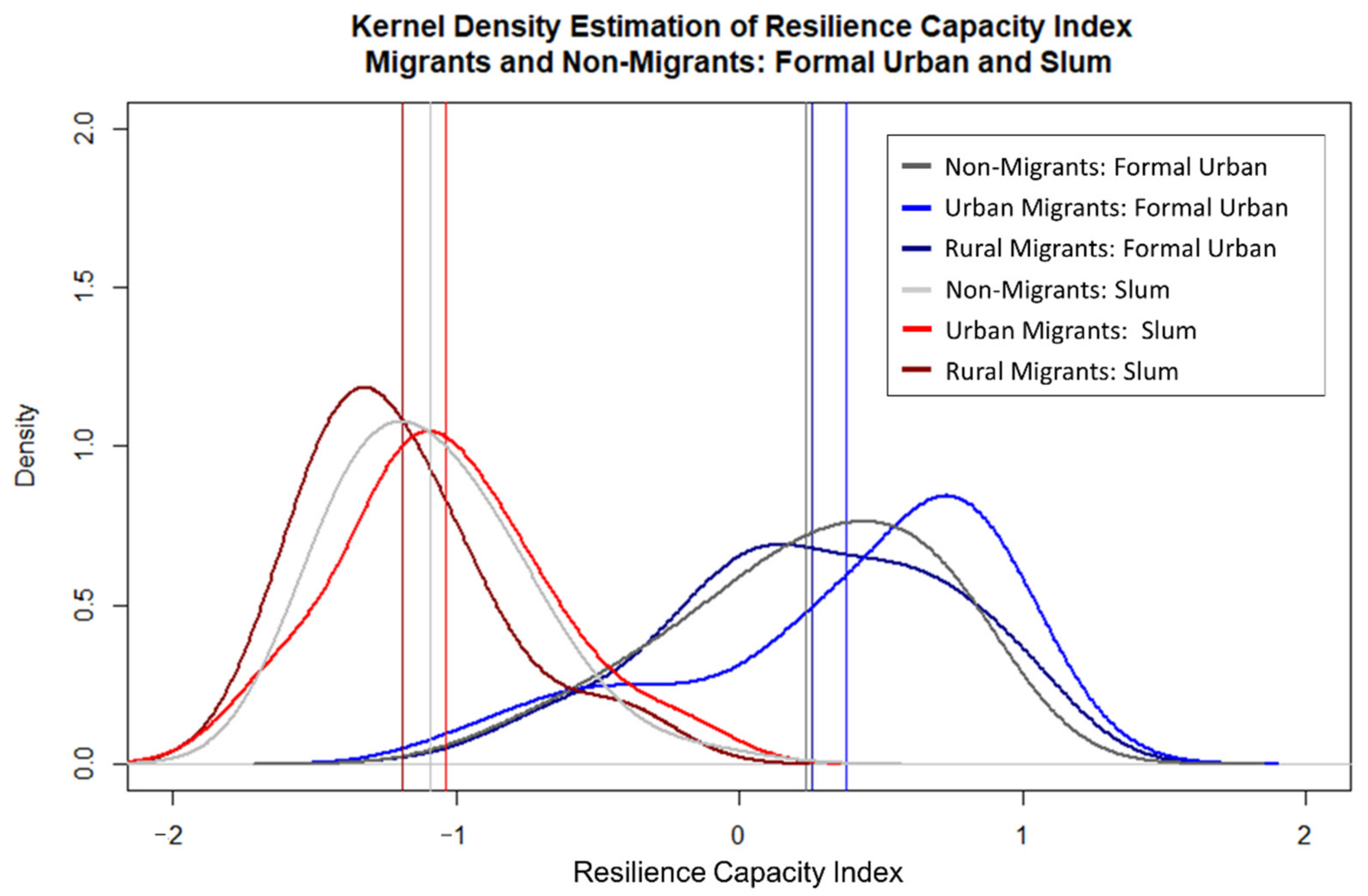
When including the additional layer of complexity by considering residence zone and migration origin, significant differences between the six previously defined sub-groups become visible (Figure 6).
Slum residents have a significantly lower resilience compared to their formal urban counterparts (p-value < 0.001). Additionally, urban migrants have a higher resilience in both residence zones compared to rural migrants and non-migrants. Migrants are on average slightly more resilient than non-migrants in the formal urban category, which does not apply to the slum category where it is the other way around (Table 2).
3.3. Intra-Migrant Comparions
Literature and HHS data provide ample evidence for the high socio-economic diversity among different migrant groups within the city [67]. Therefore, in the next section, we contrast the resilience scores against four key characteristics of migration: (1) time since arrival, (2) reasons for migration, and (3) distance travelled from the migration origin. We further analyzed (4) how the exposure to extreme weather (flood, heat) at the migration destination correlates with the households’ resilience. To allow for better comparison, we include non-migrants into the plots of the four migrant sub-groups.
3.3.1. Time since Arrival
The resilience of migrants based on the following three categories is assessed: <10, 10–20, and >20 years since arrival in Pune. When classifying migrants based on their time since arrival in Pune, distinct differences between the sub-groups appear (Figure 7, Table 3). Compared to the non-migrant sub-groups, recently arrived migrants are in all cases more resilient, whereas those longest in Pune have lower resilience throughout the four sub-groups.
3.3.2. Reasons for Migration
The following reasons for migration are considered in this analysis: work, living conditions, education, and family (Figure 8, Table 4). For the two sub-groups urban-urban and rural-urban, those who moved to Pune for education reasons have the highest resilience. In contrast, among both migrant groups living in slums (urban-slum and rural-slum), those who moved because of family reasons have the highest resilience. While most migrants moved to Pune for work reasons, their resilience tends to be one of the lowest, especially for migrants living in slums.
3.3.3. Migration Distance
The resilience of migrants based on their migration distance is compared using the categories same district, same state but other districts, and other states (Figure 9, Table 5). For the urban-urban sub-group, migrants from other states have the highest resilience whereas rural-urban migrating from other states have the lowest resilience. For both sub-groups of rural migrants, those who migrated shorter distances (same district, same state) have a higher resilience than migrants who migrated longer distances (other states).
3.3.4. Environmental Exposure: Flood and Heat
The resilience of migrants to environmental exposure is assessed based on (1) whether they experienced a flood event or not and (2) on their exposure to extreme heat events (high or low exposure) in the last three years in Pune.
Regarding floods, according to the HHS data (cf. SM, Figure S11), a higher share of migrants (5.6%) compared to non-migrants (2.1%) has been exposed to floods in the past. Again, it is especially the rural migrants who are prone to floods (rural migrants: 7.5%, urban migrants: 3.1%). Furthermore, the RM shows that flood exposure tends to reduce the resilience of migrants and non-migrants considerably, except for the urban-urban sub-group, where the opposite effect is found (Figure 10, Table 6).
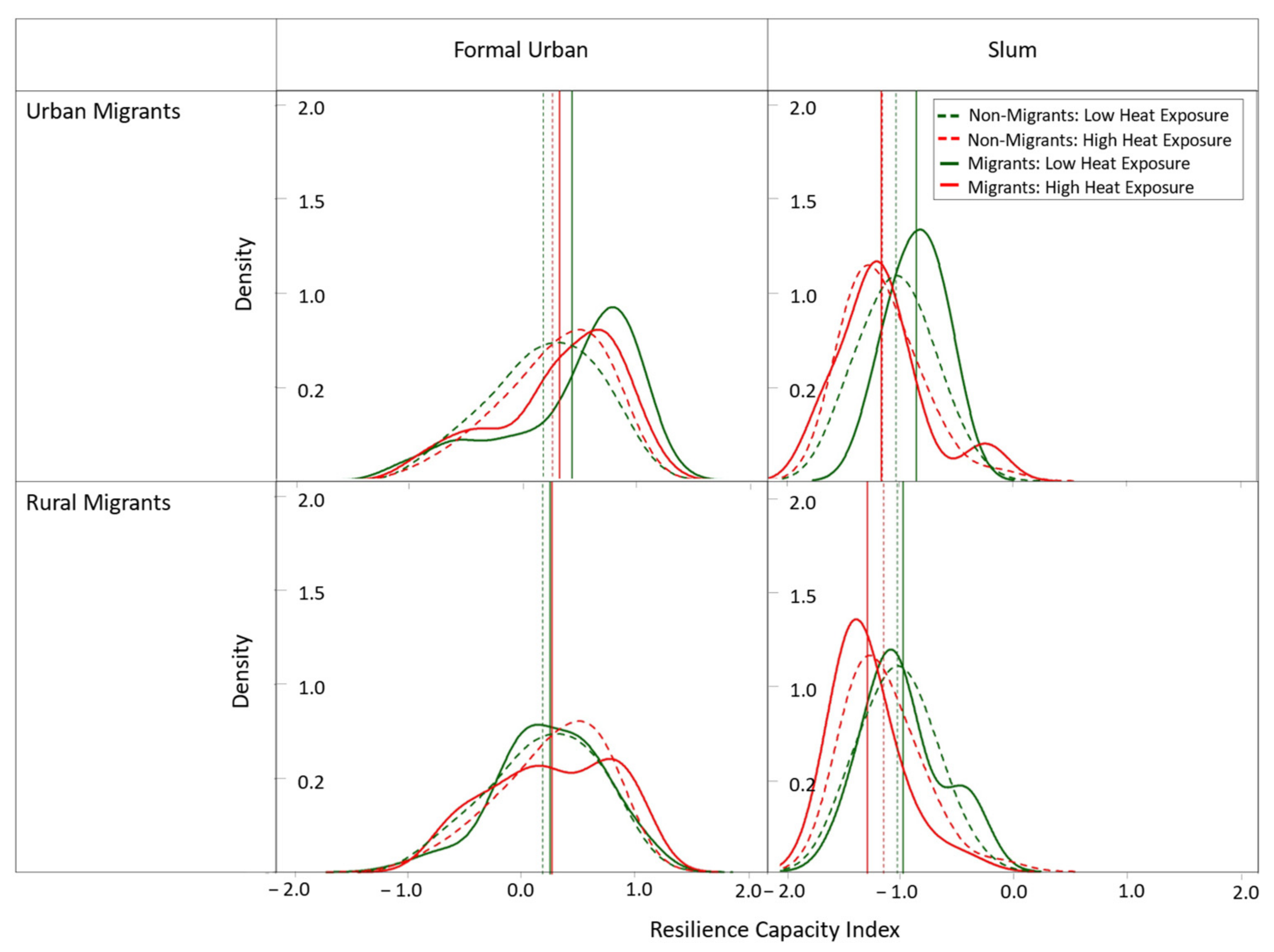
Regarding heat stress, the interpolated extreme day surface temperature map of Pune shows distinct spatial and temporal differences (cf. SM, Figure S12) with heat islands as well as areas of low extreme temperature exposure. Overall, the west of Pune tends to experience more extreme day temperatures compared to the east.
A higher share of migrants (23%) compared to non-migrants (15%) experiences high heat exposure (cf. SM, Figure S13). Among migrants, it is rural migrants who are more prone to high heat exposure than urban migrants (rural migrants: 24%, urban migrants: 14%). In general, a higher heat exposure leads to a lower resilience except for the non-migrant-urban sub-group where the opposite effect can be observed. Especially for rural-slum migrants, higher heat exposure is associated with a significantly lower resilience (p < 0.01) compared to low heat exposure (Figure 11, Table 7).
4. Discussion
The results of our RM show how the livelihood resilience of urban households is shaped by migration biographies. Several findings are of particular interest. First, resilience can vary greatly on small spatial scales, from neighborhood to neighborhood, which is linked with high differences in the availability of livelihood opportunities [68] and the nested, often informal built environment in cities such as Pune [69]. Second, comparing the total migration and non-migration cohorts, we noted a significantly higher resilience of those that have moved to Pune than those that were born in the city. On the one side, this finding is consistent with the comparisons of migrants and non-migrants by Revathy et al. [50] and Haan [70] but contrary to Foresight’s [9] assessment of migrants to be a particularly vulnerable urban group. The prior found that migrants tend to perform well in urban labor markets mainly due to higher levels of education and advantageous age cohorts [71]. The latter argues that they often lack the human, social, or financial capital to protect themselves from the environmental risks in high-density settlements where they predominantly live. This apparent contradiction is reflected in our third main finding, showing that the high resilience of migrants is accounted for only by urban migrants while rural migrants have a slightly lower resilience than the non-migrant sub-group. Acknowledging this difference is critical, albeit often neglected in research and policy—as it points to the need to differentiate between migrant biographies.
The higher resilience of urban migrants compared to rural migrants is linked with higher levels in terms of income, education, residence zone, and housing quality which relates to research by Oberai [72] who presents evidence that the poor have a comparatively greater propensity to out-migrate from rural areas than the poor from urban areas. Additionally, according to Srivastava [73] nearly half of rural migrants are found at the bottom six consumption deciles and work predominantly as casual wage employed or as self-employed in the informal sector. As a result, they tend to have no civic identity and citizenship at the destination, limited access to housing and basic amenities, poor entitlements, deficient workplace conditions, and experience labor market discrimination [74]. Moreover, we found that rural migrants perform better compared to urban migrants in one of the input variables of the RM, namely in the availability of electricity backup. On the one side, this can be interpreted as a sign of increased resilience but also a sign for the higher necessity of having electricity backup since electricity is unreliable [75].
For the investigation of the four migration characteristics, we disaggregated the sample into six sub-groups displayed in the result matrices:
First, we found an inverse relationship between time since arrival at the destination and resilience for all migrant sub-groups. This contradicts the widespread assumption that migrants need time at their new migration destination to settle and establish themselves [76]. A possible explanation for this pattern may be past peaks of rural-urban migration to Pune (the last around the year 2000) due to severe droughts. These caused a major, unplanned migrant influx to Pune, especially to the city’s slums (cf. SM, Figure S2). The HHS data suggests that more recently, the decision to leave the rural origin and move to the city may have been better planned and less displacement-driven (cf. SM, Figure S3). Nevertheless, Revi [77] highlights that climate change is expected to increase the occurrences and intensities of droughts in western India which may force more landless, small, and marginal farmers to migrate to the city’s informal neighborhoods. These rural-urban migrants are specifically vulnerable as previously described since they tend to have low human and financial capital while predominantly living in slums which are associated with higher environmental risks.
Second, marked differences between the sub-groups are examined regarding the correlation between reasons for migration and resilience: formal urban migrants score highest when motivated by education and slum-based migrants when migrating due to family reasons. We see that the prior sub-group is dominated by young migrants with high financial capital that allows them to pursue further educational attainment (human capital). The importance of family for the latter sub-group’s resilience supports the argument that networks through relationships of friendship and mutual origin are critical [78].
Third, comparing the effects of migration distance across the sub-groups, we find that while urban-urban migrants from other states feature the highest resilience, the exact opposite is the case for the rural-slum sub-group, where migrants from the same district have the highest resilience. The HHS (cf. SM, Figure S4) and evidence from literature suggest an inversely proportional relationship between migration flows and the distance between regions [79]. Possible earnings, distances, transportation costs, information on job opportunities, and psychic costs are weighed against each other. The higher financial and human capital of urban-urban migrants allows them to travel farther distances whereas rural migrants, especially those that live in the slums of Pune, have low financial and human capital and thus fewer means to travel long distances. This may serve as an explanation for these oppositional findings.
Fourth, considering Pune’s increasing exposure to extreme weather events it is alarming to see how all migrant sub-groups have greater environmental exposure than the non-migrant sub-groups, especially because exposure to floods or heat is generally correlated with lower resilience scores. It should be noted that the most resilient migrant group (urban-urban) is not significantly affected by extreme events. On the contrary, we see the paradoxical effect of higher resilience when exposed to floods. An explanation for this could be that they received compensation after the floods, irrespective of their losses, which may have been comparatively low. This, however, would need further investigation. Moreover, the rural-slum sub-group, on the other side, was severely affected both by floods and extreme heat, underlining its particularly high vulnerability. These results are supported by literature since rural-urban migrants tend to predominantly live-in slums which are linked with lower housing quality. Therefore, this sub-group’s housing does not only provide less protection during extreme weather events such as strong winds or floods but is also destroyed more quickly and easily [49,80].
In summary, the subdivision of migrants in matrices by residence zone and migration origin yields two contrasting archetypical migrant groups in Pune: First, those that live in formal urban areas with urban migration origin, and second, those that live in slums with rural migration origins. On the one side, we find that in the first, most resilient group, the highest-scoring ones have moved recently to Pune and came from far (outside Maharashtra). This group was attracted by Pune’s excellent education and the potentially good living conditions—the city has recently been ranked most livable in India by the Ministry of Housing and Urban Affairs [81]. On the other side, we find that those households have the lowest resilience who have moved from villages outside Maharashtra to Pune’s slums long ago and came to find work in the city. Other, less clear-cut archetypes may be slum households that recently came from another city within Maharashtra for family or work reasons (relatively high resilience), or those settling in slum areas after leaving the village due to living conditions (relatively low resilience).
Furthermore, it needs to be highlighted that the livelihood resilience concept serves as an important input for the RM since it provides relevant insights into quantifying the resilience of different sub-groups with and without migration backgrounds. Its detailed conceptual and analytical framework makes it particularly suitable for translation into a quantitative model on urban migrants’ resilience. Related concepts such as social resilience [18] or translocal social resilience [82], so far, either lack relevant aspects regarding the migration context or are too complex to be implemented in an RM [17].
Overall, the data shows how diverse and complex migration patterns and the associated household resilience are. While the clustering into stylized archetypes may help for a better understanding of qualitatively different groups, a categorization can never be absolute and should be treated with caution. Additional limitations of our RM include a limited sample size of the HHS, incomplete data on water and electricity access, quality, and quantity, as well as a lack of predictor variables. All the above resulted in both a limited number of pillars and prevented a quantification of indirect resilience. Moreover, two specific methodological shortcomings of quantitative resilience approaches are recognized: first, a possible arbitrariness in the selection of input and predictor variables, and second, the challenges of accounting for the socio-cultural contexts in which resilience occurs. Furthermore, a statistical model can never capture the multi-facetted resilience complexity of urban households completely and we need to be cautious with causal inferences. Despite these limitations, we argue that our presented RM can provide valuable insights for policymakers to set and implement targeted resilience interventions.
5. Conclusions
This study shows that on average households with migration backgrounds are more resilient than households without. More importantly, we show that not migration, as such, but the migration biography matters. In particular, migrants’ residence zone at the migration destination, migration origin, migration distance, time since arrival at the destination, and the reasons for migration strongly influence households’ resilience and affectedness by extreme weather events. Only by including characteristics from the migration biographies, we detect the significant differences between rural and urban migrants and the impact of the residence zone, time since arrival or distance migrated on resilience. Our results thus paint a multi-faceted picture of Pune’s migrant population which contradicts simplistic notions of migrants as socio-economic “high-performers” or “problem children.”
The resilience of households in rapidly growing cities to environmental hazards is rising in importance: The exposed population is growing as well as the frequency and intensity of extreme weather events. Especially for emerging megacities across the world, efforts towards actively increasing urban household resilience are needed to allow for sustainable economic and demographic growth. While our results describe the situation in Pune, the approach can be applied to any other city facing large migration influx, urban informality, and natural hazards. This study provides valuable information for policymakers on the resilience structure of urban households with a specific focus on migrants, enhancing the targeting and effectiveness of resilience interventions. On the one side, our RM fosters the understanding of policymakers on the resilience of particular population groups and the reasons for it. On the other side, it can be used to estimate the resilience effects of specific proactive and reactive interventions.
Therefore, in the future, resilience research in Pune and other cities of the Global South should be continued using similar surveys to establish a time-series data set while addressing the previously established limitations. This can be achieved, for example, by increasing the sample size to decrease standard deviation and uncoverage bias. Additionally, expanding the comprehensives of the RM by including important insights from, for example, the social resilience and translocal social resilience concepts as well as environmental factors (vegetation) from remote sensing data could provide valuable insights into resilience dynamics. Moreover, future research should aim to implement a mixed-method design since the combination of quantitative and qualitative data allows for a more layered analysis at varying depths of meaning. The qualitative data could allow to test the accuracy of the RM results as well as reveal which additional parameters might have to be included in the RM.
Finally, we advocate that both policymakers and scientists account for migration biographies in assessments of resilience and adjacent concepts such as vulnerability and livability. The socio-economic and cultural properties are too diverse to justify treating migrants as one homogeneous group. Neglecting migration biographies can lead to the implementation of ineffective resilience interventions and an associated misallocation of scarce funds. Endeavors such as the RM presented in this work can lay the ground for sustaining the resilience of urban households in rapidly-growing cities despite the dual pressure of elevating urbanization and climate-change-induced hazards.
Supplementary Materials
The following are available online at www.mdpi.com/article/10.3390/land10111134/s1, Supplementary Material: 1. HHS, 1.1 Data Collection, 1.2 Reasons for Migration, 1.3 Descriptive Statistics, 2. Model, 2.1 Data Processing, 2.2 Structure, 2.3 Testing Resilience Interventions with Model, 2.4 Pillars, 2.4.1 Assets, 2.4.2 Housing, 2.4.3 Health, 3. Migration Characteristics, 3.1 Flood Exposure, 3.2 Heat Exposure, and 3.3 Experiments with environmental data. Figure S1: Reasons for migration categories used in HHS, Figure S2: (a) Yearly number of migrants in Pune and (b) yearly number of migrants in Pune’s formal urban areas and slums (1924–2019) based on HHS, Figure S3: Share of Urban and Rural Migrants for years since arrival categories, Figure S4: Origin of migration of Pune migrants based on HHS, Figure S5: Path diagram of hierarchical Resilience Model based on assets (ass), housing (hos), health (hlt) where circles represent latent variables, rectangles observable variables, Figure S6: Path diagram of Structural Equation Model displaying how each pillar relates to resilience, Figure S7: Resilience Structure Matrix of three pillars assets, housing, and health, Figure S8: Figures of descriptive statistics of assets pillar (income, education, and food–income ratio) for migrant, urban migrant, rural migrant, and non-migrant, Figure S9: Figures of descriptive statistics of housing pillar (zone, dwelling, rooms, and space) for migrant, urban migrant, rural migrant, and non-migrant, Figure S10: Figures of descriptive statistics of health pillar (flush toilet, total water storage, total cooling devices, and electricity backup) for migrant, urban migrant, rural migrant, and non-migrant, Figure S11: Percentage of flood-affected households (migrant, urban migrant, rural migrant, and non-migrant), Figure S12: Interpolation of extreme temperature experiences per household (90th percentile), Figure S13: Heat exposure (low, middle, high) experienced by different focus groups (migrant, urban migrant, rural migrant, and non-migrant), Table S1: Categories and Indicators of the Resilience Model, Table S2: Tables of descriptive statistics of assets pillar (income, education, and food–income ratio) for migrant, urban migrant, rural migrant, and non-migrant (* low sample size), Table S3: Tables of descriptive statistics of housing pillar (zone, dwelling, space, and rooms) for migrant, urban migrant, rural migrant, and non-migrant (* low sample size), Table S4: Figures of descriptive statistics of health pillar (flush toilet, total water storage, total cooling devices, and electricity backup) for migrant, urban migrant, rural migrant, and non-migrant (* low sample size).
Author Contributions
Conceptualization, A.-C.L.; Data curation, A.-C.L., Y.Z. and R.K.; Formal analysis, A.-C.L.; Investigation, A.-C.L.; Methodology, A.-C.L.; Software, A.-C.L.; Supervision, R.K.; Visualization, A.-C.L.; Writing—original draft, A.-C.L. and R.K.; Writing—review & editing, Y.Z. and R.K. All authors have read and agreed to the published version of the manuscript.
Funding
This work was conducted as part of the Belmont Forum Sustainable Urbanisation Global Initiative (SUGI)/Food-Water-Energy Nexus theme for which coordination was supported by the US National Science Foundation under grant ICER/EAR-1829999 to Stanford University. UFZ received funding from the Federal Ministry of Education and Research (BMBF) under grant 033WU002. Any opinions, findings, and conclusions, or recommendations expressed in this material do not necessarily reflect the views of the funding organizations.
Institutional Review Board Statement
Ethical review and approval were waived for this study. This study does not involve animals. The involvement of humans occurred during the survey data collection process. The data collection was conducted strictly in accordance with the European General Data Protection Regulation. Only non-sensitive personal data was collected and analyzed. All data has been treated confidentially.
Informed Consent Statement
Informed consent was obtained from all subjects involved in the study verbally. No written informed consent is available since the survey interviews were collected anonymously. All the interviews were conducted under the condition that verbal informed consent of the respondent was obtained.
Data Availability Statement
The data presented in this study are available on request from the corresponding author. The data are not publicly available due to privacy regulations with regards to the households survey results.
Acknowledgments
The authors are grateful to Christian Kuhlicke, Eberhard Rothfuß, and Sigrun Kabisch for their supervision and feedback. The authors would also like to extend their gratitude to Vishal Gaikwad and his team from the Gokhale Institute of Politics and Economics, Pune for data collection and cleaning, and two anonymous reviewers for helpful feedback.
Conflicts of Interest
The authors declare no conflict of interest. The funders had no role in the design of the study; in the collection, analyses, or interpretation of data; in the writing of the manuscript, or in the decision to publish the results.
References
- United Nations Department of Economic and Social Affairs. World Urbanization Prospects: The 2014 Revision: Highlights; United Nations: New York, NY, USA, 2014; Available online: https://population.un.org/wup/Publications/Files/WUP2014-Highlights.pdf (accessed on 31 May 2021).
- United Nations Migration Agency. Who Is a Migrant? Available online: https://www.iom.int/who-is-a-migrant (accessed on 31 May 2021).
- International Migration Organization. World Migration Report 2020; United Nations: Geneva, Switzerland, 2019; ISBN 9789290687894. [Google Scholar]
- Perch-Nielsen, S.L.; Bättig, M.B.; Imboden, D. Exploring the link between climate change and migration. Clim. Chang. 2008, 91, 375–393. [Google Scholar] [CrossRef]
- Eckstein, D.; Künzel, V.; Schäfer, L. Global Climate Risk Index 2021: Who Suffers Most from Extreme Weather Events? Weather-Related Loss Events in 2019 and 200-2019. 2021. Available online: https://germanwatch.org/sites/default/files/Global%20Climate%20Risk%20Index%202021_2.pdf (accessed on 22 June 2021).
- Hoffmann, R.; Dimitrova, A.; Muttarak, R.; Crespo Cuaresma, J.; Peisker, J. A meta-analysis of country-level studies on environmental change and migration. Nat. Clim. Chang. 2020, 10, 904–912. [Google Scholar] [CrossRef]
- Kainth, G.S. Push and Pull Factors of Migration: A Case of Brick Kiln Industry of Punjab State; Asia Pacific Journal of Social Sciences: Bengaluru, India, 2009. [Google Scholar]
- WBGU. World in Transition: Climate Change as a Security Risk; Summary for Policymakers; Wissenschaftlicher Beirat d. Bundesregierung Globale Umweltveränderungen: Berlin, Germany, 2007; ISBN 978-3-936191-20-2. [Google Scholar]
- Foresight. Migration and Global Environmental Change (Final Project Report); The Government Office for Science: London, UK, 2011.
- Mallick, B. The Nexus between Socio-Ecological System, Livelihood Resilience, and Migration Decisions: Empirical Evidence from Bangladesh. Sustainability 2019, 11, 3332. [Google Scholar] [CrossRef] [Green Version]
- Cutter, S.L.; Barnes, L.; Berry, M.; Burton, C.; Evans, E.; Tate, E.; Webb, J. A place-based model for understanding community resilience to natural disasters. Glob. Environ. Chang. 2008, 18, 598–606. [Google Scholar] [CrossRef]
- Holling, C. Resilience and Stability of Ecological Systems. Annu. Rev. Ecol. Syst. 1973, 4, 1–23. [Google Scholar] [CrossRef] [Green Version]
- Hayward, B.M. Rethinking Resilience: Reflections on the Earthquakes in Christchurch, New Zealand, 2010 and 2011. Ecol. Soc. 2013, 18, 6. [Google Scholar] [CrossRef] [Green Version]
- Brown, K. Global environmental change I: A social turn for resilience? Prog. Hum. Geogr. 2014, 38, 107–117. [Google Scholar] [CrossRef] [Green Version]
- O’Brien, K. Responding to environmental change: A new age for human geography? Prog. Hum. Geogr. 2011, 35, 542–549. [Google Scholar] [CrossRef]
- Weichelsgartner, J.; Kelman, I. Geographies of resilience: Challenges and opportunities of a descriptive concept. Prog. Hum. Geogr. 2015, 39, 249–267. [Google Scholar] [CrossRef] [Green Version]
- Speranza, C.I.; Wiesmann, U.; Rist, S. An indicator framework for assessing livelihood resilience in the context of social–ecological dynamics. Glob. Environ. Chang. 2014, 28, 109–119. [Google Scholar] [CrossRef]
- Adger, N.W. Social and ecological resilience: Are they related? Prog. Hum. Geogr. 2000, 43, 347–364. [Google Scholar] [CrossRef]
- Chambers, R.; Conway, G. Sustainable Rural Livelihoods: Practical Concepts for the 21st Century; Institute of Development Studies: Sussex, UK, 1992. [Google Scholar]
- de Haan, L.J.; Zoomers, A. Exploring the Frontier of Livelihoods Research. Dev. Chang. 2005, 36, 27–47. [Google Scholar] [CrossRef]
- Marschke, M.J.; Berkes, F. Exploring Strategies that Build Livelihood Resilience: A Case from Cambodia. Ecol. Soc. 2006, 11, 16. [Google Scholar] [CrossRef] [Green Version]
- Pingali, P.; Alinovi, L.; Sutton, J. Food security in complex emergencies: Enhancing food system resilience. Disasters 2005, 29 (Suppl. 1), S5–S24. [Google Scholar] [CrossRef]
- FAO. Measuring Resilience: A Concept Note on the Resilience Tool. Food Secur. Inf. Decis. Mak. Concept Note 2012, 1–4. Available online: https://www.fao.org/resilience/resources/resources-detail/en/c/317275/ (accessed on 22 October 2021).
- Alinovi, L.; Mane, E.; Romano, D. Measuring Household Resilience to Food Insecurity: Application to Palestinian Households. In Agricultural Survey Methods; Benedetti, R., Ed.; John Wiley & Sons: Chichester, UK, 2008; pp. 1–35. ISBN 9780470665480. [Google Scholar]
- D’Errico, M.; Di Giuseppe, S.; Pietrelli, R.; Grazioli, F. Resilience Analysis in Mali: FAO Resilience Analysis No. 4; FAO: Rome, Italy, 2015. [Google Scholar]
- D’Errico, M.; Di Giuseppe, S.; Pietrelli, R.; Grazioli, F. Resilience Analysis in Niger: FAO Resilience Analysis No. 3; FAO: Rome, Italy, 2015. [Google Scholar]
- Ciani, F.; Romano, D. Testing for Household Resilience to Food Insecurity: Evidence from Nicaragua 1053-2016-85948. 2014. Available online: https://ageconsearch.umn.edu/record/172958/ (accessed on 10 September 2021).
- FAO. Resilience Index Measurement and Analysis II-RIMA-II. Food Agric. Organ. United Nations 2016 2016, 1–80. Available online: https://www.preventionweb.net/publication/rima-ii-resilience-index-measurement-and-analysis-ii (accessed on 22 October 2021).
- Kozlowska, K.; D’Errico, M.; Pietrelli, R.; Di Giuseppe, S. Resilience Analysis in Burkina Faso 1998–2003; FAO: Rome, Italy, 2015. [Google Scholar]
- D’Errico, M.; Romano, D.; Pietrelli, R. Household resilience to food insecurity: Evidence from Tanzania and Uganda. Food Sec. 2018, 10, 1033–1054. [Google Scholar] [CrossRef]
- Dhar, T.K.; Khirfan, L. A multi-scale and multi-dimensional framework for enhancing the resilience of urban form to climate change. Urban Clim. 2017, 19, 72–91. [Google Scholar] [CrossRef]
- Gonzales, P.; Ajami, N.K. An integrative regional resilience framework for the changing urban water paradigm. Sustain. Cities Soc. 2017, 30, 128–138. [Google Scholar] [CrossRef] [Green Version]
- Chun, H.; Chi, S.; Hwang, B. A Spatial Disaster Assessment Model of Social Resilience Based on Geographically Weighted Regression. Sustainability 2017, 9, 2222. [Google Scholar] [CrossRef] [Green Version]
- Kotzee, I.; Reyers, B. Piloting a social-ecological index for measuring flood resilience: A composite index approach. Ecol. Indic. 2016, 60, 45–53. [Google Scholar] [CrossRef]
- Joerin, J.; Shaw, R.; Takeuchi, Y.; Krishnamurthy, R. The adoption of a climate disaster resilience index in Chennai, India. Disasters 2014, 38, 540–561. [Google Scholar] [CrossRef] [PubMed]
- Suárez, M.; Gómez-Baggethun, E.; Benayas, J.; Tilbury, D. Towards an Urban Resilience Index: A Case Study in 50 Spanish Cities. Sustainability 2016, 8, 774. [Google Scholar] [CrossRef] [Green Version]
- Abdrabo, M.A.; Hassaan, M.A. An integrated framework for urban resilience to climate change—Case study: Sea level rise impacts on the Nile Delta coastal urban areas. Urban Clim. 2015, 14, 554–565. [Google Scholar] [CrossRef]
- Gaillard, J.C.; Walters, V.; Rickerby, M.; Shi, Y. Persistent Precarity and the Disaster of Everyday Life: Homeless People’s Experiences of Natural and Other Hazards. Int. J. Disaster Risk Sci. 2019, 10, 332–342. [Google Scholar] [CrossRef] [Green Version]
- Gardner, J.S.; Dekens, J. Mountain hazards and the resilience of social–ecological systems: Lessons learned in India and Canada. Nat. Hazards 2006, 41, 317–336. [Google Scholar] [CrossRef]
- Gautam, Y. Seasonal Migration and Livelihood Resilience in the Face of Climate Change in Nepal. Mt. Res. Dev. 2017, 37, 436–445. [Google Scholar] [CrossRef] [Green Version]
- Brenkert, A.L.; Malone, E.L. Modeling Vulnerability and Resilience to Climate Change: A Case Study of India and Indian States. Clim. Chang. 2005, 72, 57–102. [Google Scholar] [CrossRef]
- Deshingkar, P. Environmental risk, resilience and migration: Implications for natural resource management and agriculture. Environ. Res. Lett. 2012, 7, 15603. [Google Scholar] [CrossRef]
- Das, S.; DSouza, N.M. Identifying the local factors of resilience during cyclone Hudhud and Phailin on the east coast of India. Ambio 2020, 49, 950–961. [Google Scholar] [CrossRef]
- Duncan, J.M.; Tompkins, E.L.; Dash, J.; Tripathy, B. Resilience to hazards: Rice farmers in the Mahanadi Delta, India. Ecol. Soc. 2017, 22, 3. [Google Scholar] [CrossRef] [Green Version]
- Birthal, P.S.; Hazrana, J. Crop diversification and resilience of agriculture to climatic shocks: Evidence from India. Agric. Syst. 2019, 173, 345–354. [Google Scholar] [CrossRef]
- Nayak, P.K.; Oliveira, L.E.; Berkes, F. Resource degradation, marginalization, and poverty in small-scale fisheries: Threats to social-ecological resilience in India and Brazil. Ecol. Soc. 2014, 19, 13. [Google Scholar] [CrossRef] [Green Version]
- Census of India. D3—Migrants by Place of Last Residence and Reasons for Migration-2011. 2011. Available online: https://censusindia.gov.in/DigitalLibrary/TablesSeries2001.aspx (accessed on 1 April 2021).
- Mayer, B. The Arbitrary Project of Protecting Environmental Migrants. Environmental Migration and Social Inequality; Springer: Cham, Switzerland, 2016; pp. 189–200. [Google Scholar]
- Hari, V.; Dharmasthala, S.; Koppa, A.; Karmakar, S.; Kumar, R. Climate hazards are threatening vulnerable migrants in Indian megacities. Nat. Clim. Chang. 2021, 11, 636–638. [Google Scholar] [CrossRef]
- Revathy, N.; Thilagavathi, M.; Surendran, A. A Comparative Analysis of Rural-Urban Migrants and Non-Migrants in the Selected Region of Tamil Nadu, India. Econ. Aff. 2020, 65, 23–30. [Google Scholar]
- Census of India. Pune City Population Census 2011–2021: Maharashtra. Available online: https://www.census2011.co.in/census/city/375-pune.html (accessed on 26 May 2021).
- Krishnamurthy, R.; Mishra, R.; Desouza, K.C. City profile: Pune, India. Cities 2016, 53, 98–109. [Google Scholar] [CrossRef]
- Pune Municipal Corporation. Fire Hazards Response and Mitigation Plan. 2011. Available online: http://www.pmc.gov.in/informpdf/Fire_Hazards/3annexurefinal.pdf (accessed on 22 June 2021).
- Cronin, V.; Guthrie, P. Community-led resettlement: From a flood-affected slum to a new society in Pune, India. Environ. Hazards 2011, 10, 310–326. [Google Scholar] [CrossRef]
- Shinde, K.A. Disruption, resilience, and vernacular heritage in an Indian city: Pune after the 1961 floods. Urban Stud. 2017, 54, 382–398. [Google Scholar] [CrossRef]
- PTI. Intense Rain Pounds Pune; 17 Killed, Nearly 16,000 Rescued. Economic Times [Online], 26 September 2019. Available online: https://economictimes.indiatimes.com/news/politics-and-nation/flooding-in-pune-after-heavy-rain-7-killed-500-rescued/articleshow/71306297.cms(accessed on 11 March 2021).
- ET Online. Mutha Canal Wall Collapse Floods Dandekar Bridge Area in Pune. Economic Times [Online], 27 September 2018. Available online: https://economictimes.indiatimes.com/news/politics-and-nation/mula-canal-wall-collapse-floods-dandekar-bridge-area-in-pune/articleshow/65978344.cms(accessed on 11 March 2021).
- Sharma, S.; Mujumdar, P. Increasing frequency and spatial extent of concurrent meteorological droughts and heatwaves in India. Sci. Rep. 2017, 7, 15582. [Google Scholar] [CrossRef] [Green Version]
- Correspondent, H. IMD Issues Heatwave Warning for Pune. Hindustan Times [Online], 20 May 2019. Available online: https://www.hindustantimes.com/pune-news/imd-issues-heatwave-warning-for-pune/story-uk4ZYpQDwjA8hGyID1eitK.html(accessed on 19 March 2021).
- Gautam, A. At 42.9 Degrees Pune in Maharashtra Breaks Record of Last 36 Years. Skymet Weather Services [Online], 28 April 2019. Available online: https://www.skymetweather.com/content/weather-news-and-analysis/at-42-9-degrees-pune-in-maharashtra-breaks-record-of-last-36-years/(accessed on 19 March 2021).
- National Sample Survey Office. India—Employment, Unemployment and Migration Survey: NSS 64th Round. 2008. Available online: http://www.icssrdataservice.in/datarepository/index.php/catalog/33/data-dictionary (accessed on 8 October 2021).
- Alinovi, L.; D’Errico, M.; Mane, E.; Romano, D. Livelihood strategies and household resilience to food insecurity: An empirical analysis to Kenya. In Proceedings of the Conference on “Promoting Resilience through Social Protection in Sub-Saharan Africa, Dakar, Senegal, 28–30 June 2010. [Google Scholar]
- Oriangi, G.; Bamutaze, Y.; Mukwaya, P.I.; Musali, P.; Di Baldassarre, G.; Pilesjö, P. Testing the Proposed Municipality Resilience Index to Climate Change Shocks and Stresses in Mbale Municipality in Eastern Uganda. Am. J. Clim. Chang. 2019, 8, 520–543. [Google Scholar] [CrossRef] [Green Version]
- Das, P.; Mudi, S.; Behera, M.D.; Barik, S.K.; Mishra, D.R.; Roy, P.S. Automated Mapping for Long-Term Analysis of Shifting Cultivation in Northeast India. Remote Sens. 2021, 13, 1066. [Google Scholar] [CrossRef]
- Ghaderpour, E.; Ben Abbes, A.; Rhif, M.; Pagiatakis, S.D.; Farah, I.R. Non-stationary and unequally spaced NDVI time series analyses by the LSWAVE software. Int. J. Remote Sens. 2020, 41, 2374–2390. [Google Scholar] [CrossRef]
- Hazaymeh, K.; Hassan, Q.K. Remote sensing of agricultural drought monitoring: A state of art review. AIMS Environ. Sci. 2016, 3, 604–630. [Google Scholar] [CrossRef]
- Purkayastha, B. Migration, migrants, and human security. Curr. Sociol. 2018, 66, 167–191. [Google Scholar] [CrossRef]
- Jimmy, E.N.; Martinez, J.; Verplanke, J. Spatial Patterns of Residential Fragmentation and Quality of Life in Nairobi City, Kenya. Appl. Res. Qual. Life 2020, 15, 1493–1517. [Google Scholar] [CrossRef] [Green Version]
- Hernbäck, J. Influence of Urban Form on Co-Presence in Public Space: A Space Syntax Analysis of Informal Settlements in Pune, India; DiVA: Uppsala, Sweden, 2012. [Google Scholar]
- de Haan, A. Rural-Urban Migration and Poverty: The Case of India. IDS Bull. 1997, 28, 35–47. [Google Scholar] [CrossRef] [Green Version]
- Rajendran, D.; Ng, E.S.; Sears, G.; Ayub, N. Determinants of Migrant Career Success: A Study of Recent Skilled Migrants in Australia. Int. Migr. 2020, 58, 30–51. [Google Scholar] [CrossRef] [Green Version]
- Oberai, A.S. Problems of Urbanisation and Growth of Large Cities in Developing Countries: A Conceptual Framework for Policy Analysis; International Labour Organization: Geneva, Switzerland, 1989; Available online: https://econpapers.repec.org/paper/iloilowps/992668663402676.htm (accessed on 10 September 2021).
- Srivastava, R. Labour migration in India: Recent trends, patterns and policy issues. Indian J. Labour Econ. 2011, 54, 411–440. [Google Scholar]
- Sabates-Wheeler, R.; Waite, M. Migration and Social Protection: A Concept Paper; Institute of Development Studies: Sussex, UK, 2003. [Google Scholar]
- Aklin, M.; Bayer, P.; Harish, S.P.; Urpelainen, J. Quantifying slum electrification in India and explaining local variation. Energy 2015, 80, 203–212. [Google Scholar] [CrossRef] [Green Version]
- Pennix, R. Integration of Migrants: Economic, Social, Cultural and Political Dimensions; UNECE: Geneva, Switzerland, 2005. [Google Scholar]
- Revi, A. Climate change risk: An adaptation and mitigation agenda for Indian cities. Environ. Urban. 2008, 20, 207–229. [Google Scholar] [CrossRef] [Green Version]
- Brettell, C.B.; Hollifield, J.F. Migration Theory: Talking across Disciplines, 3rd ed.; Taylor and Francis: Hoboken, NJ, USA, 2014; ISBN 9781317805984. [Google Scholar]
- Boyle, P.; Halfacree, K.H.; Robinson, V. Exploring Contemporary Migration; Taylor and Francis: Hoboken, NJ, USA, 2014; ISBN 9781317890874. [Google Scholar]
- Desai, R.; Sanghvi, S. Circular Migration and Urban Housing. Handbook of Internal Migration in India; SAGE Publications Pvt Ltd.: New Delhi, India, 2020; pp. 462–475. [Google Scholar]
- Ministry of Housing and Urban Affairs. Ease of Living. 2018. Available online: http://amplifi.mohua.gov.in/eol-landing (accessed on 26 September 2021).
- Sakdapolrak, P.; Naruchaikusol, S.; Ober, K.; Peth, S.; Porst, L.; Rockenbauch, T.; Tolo, V. Migration in a changing climate. Towards a translocal social resilience approach. DIE ERDE–J. Geogr. Soc. Berl. 2016, 147, 81–94. [Google Scholar] [CrossRef]
Figure 1.
Total number of Pune District migrants per state of origin in 64th NSSO round 2008 (n = 1438) [61].
Figure 1.
Total number of Pune District migrants per state of origin in 64th NSSO round 2008 (n = 1438) [61].
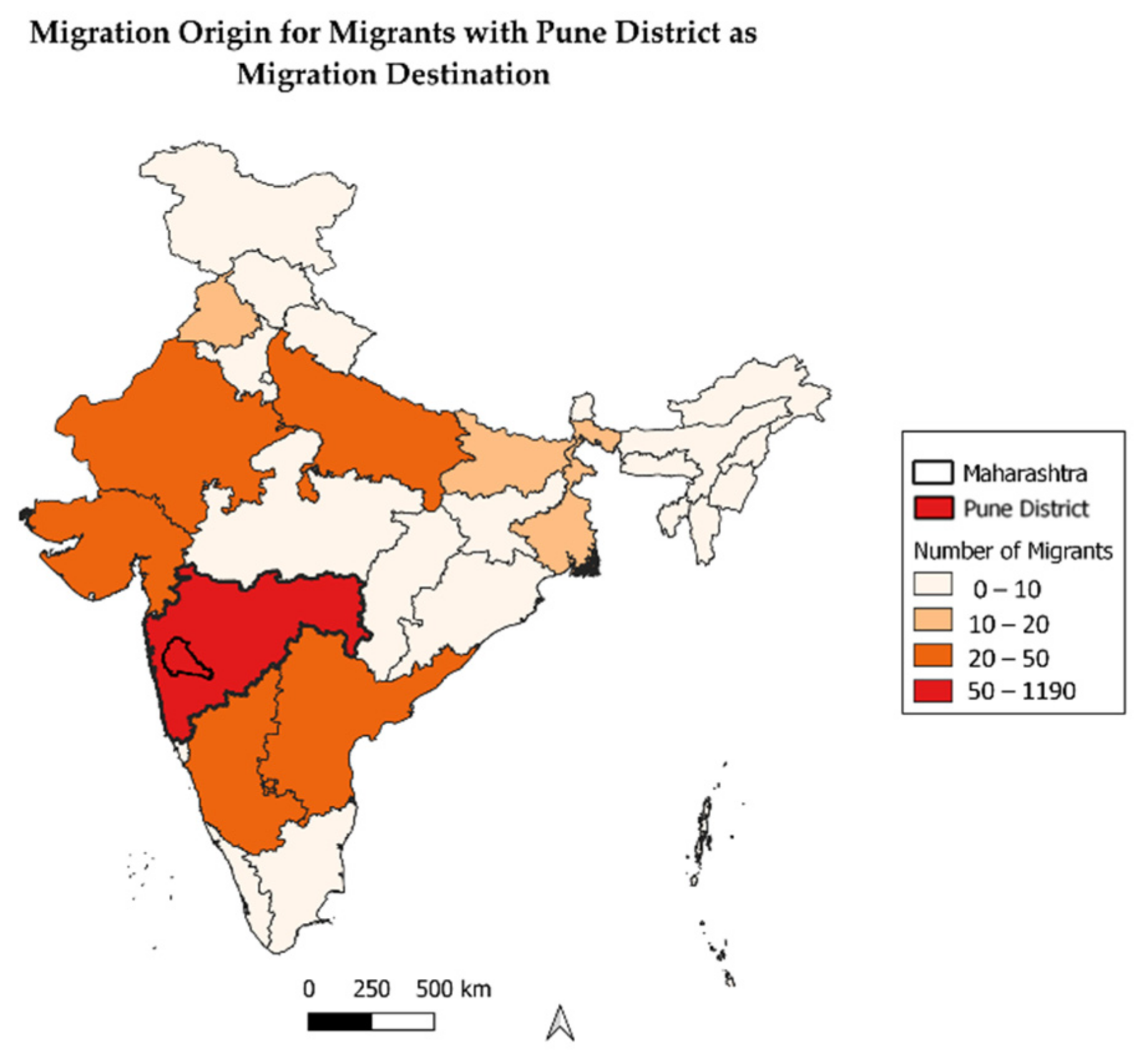
Figure 2.
Resilience model framework describing how resilience is calculated based on the three pillars: assets, housing, and health as well as their associated variables.
Figure 2.
Resilience model framework describing how resilience is calculated based on the three pillars: assets, housing, and health as well as their associated variables.
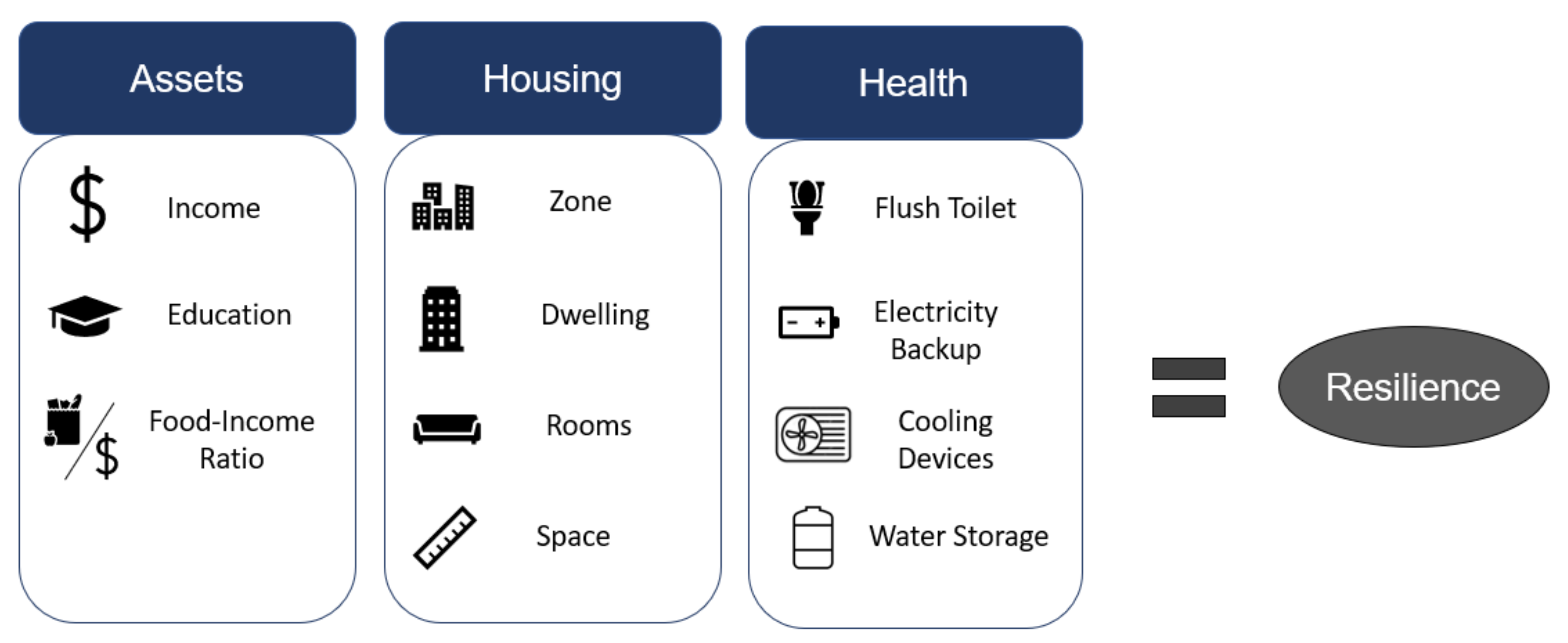
Figure 3.
Explanation of migration biography including four migration characteristics and six sub-groups from matrix.
Figure 3.
Explanation of migration biography including four migration characteristics and six sub-groups from matrix.
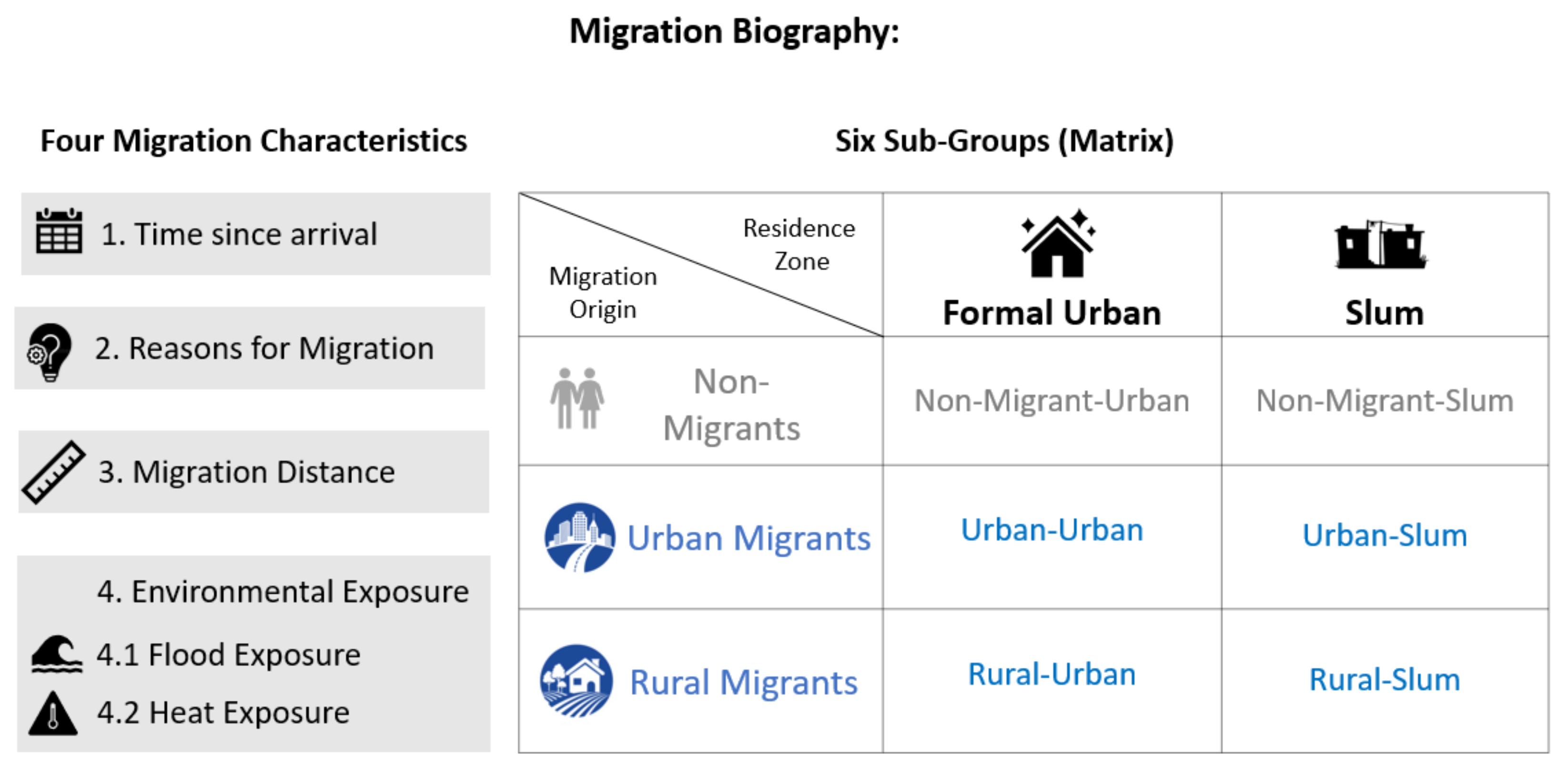
Figure 4.
Resilience capacity index of Pune households using 1000 m grids. In the zoomed-in section (purple), slums are shown hatched in red. Dots correspond to individual households. For data security reasons, locations correspond to the next street crossing, not the exact building.
Figure 4.
Resilience capacity index of Pune households using 1000 m grids. In the zoomed-in section (purple), slums are shown hatched in red. Dots correspond to individual households. For data security reasons, locations correspond to the next street crossing, not the exact building.
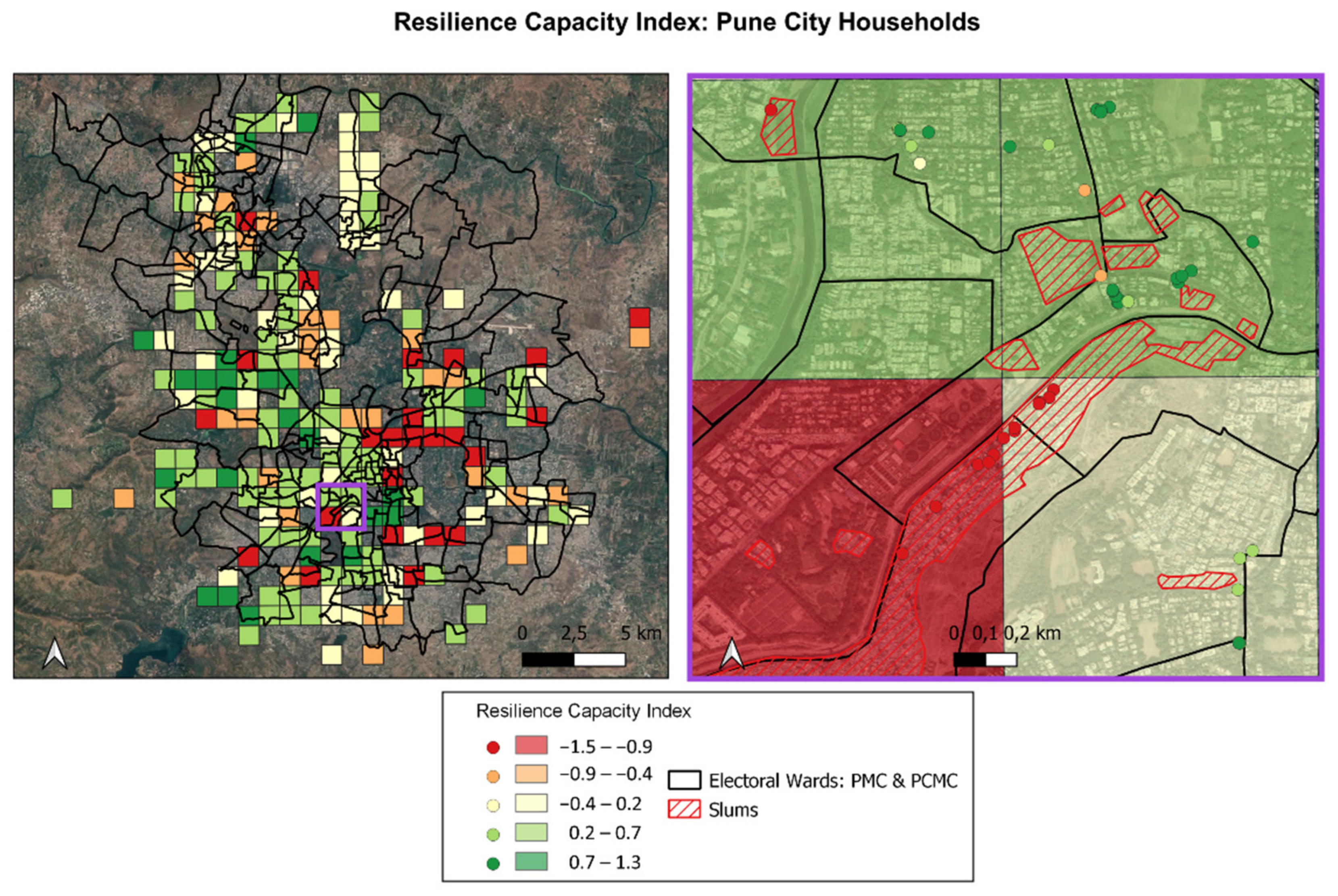
Figure 5.
Kernel density estimation of RCI: migrants (urban, rural origin) and non-migrants.
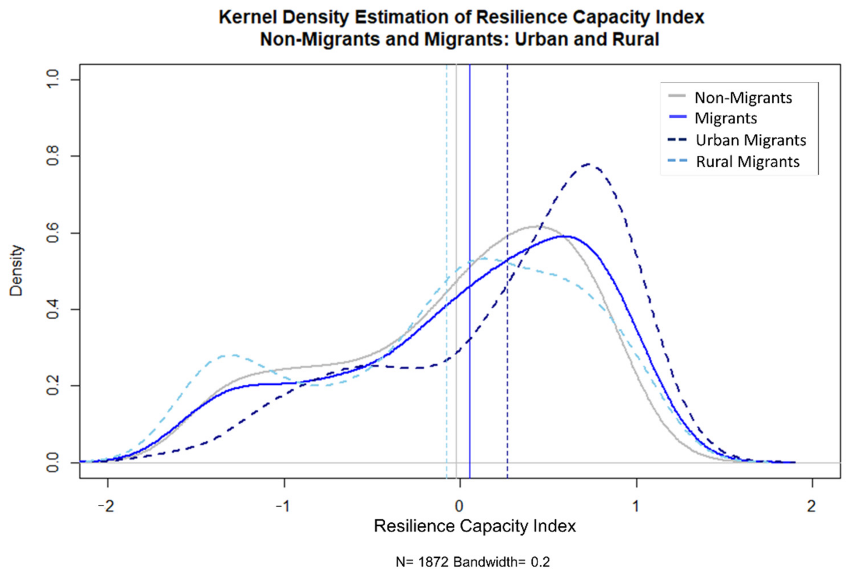
Figure 6.
Kernel density estimation of RCI for the six analyzed sub-groups.

Figure 7.
Resilience matrix displaying kernel density estimation of RCI of sub-groups based on the migration characteristic time since arrival.
Figure 7.
Resilience matrix displaying kernel density estimation of RCI of sub-groups based on the migration characteristic time since arrival.
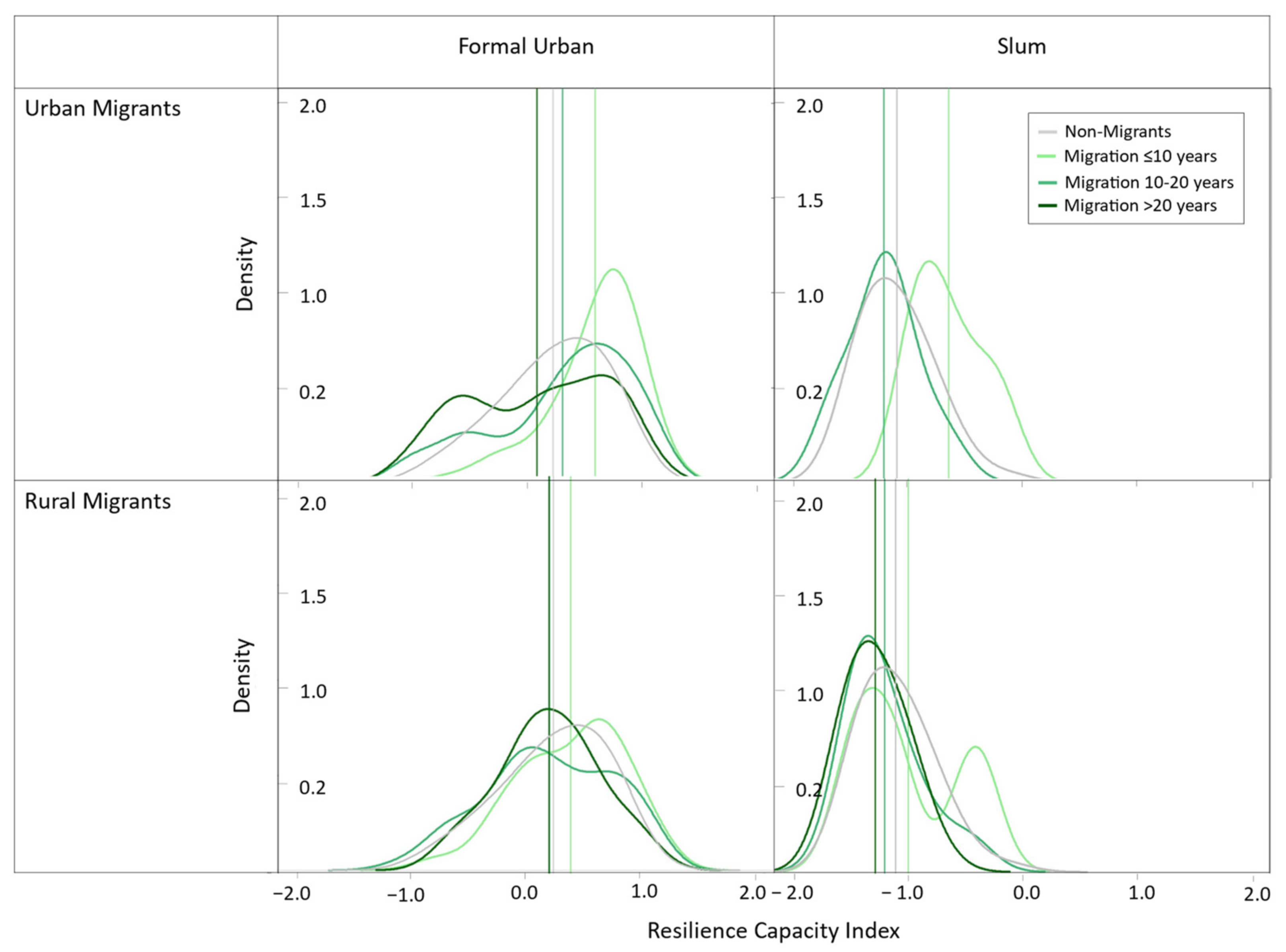
Figure 8.
Resilience matrix displaying kernel density estimation of RCI of sub-groups based on the migration characteristic reasons for migration.
Figure 8.
Resilience matrix displaying kernel density estimation of RCI of sub-groups based on the migration characteristic reasons for migration.
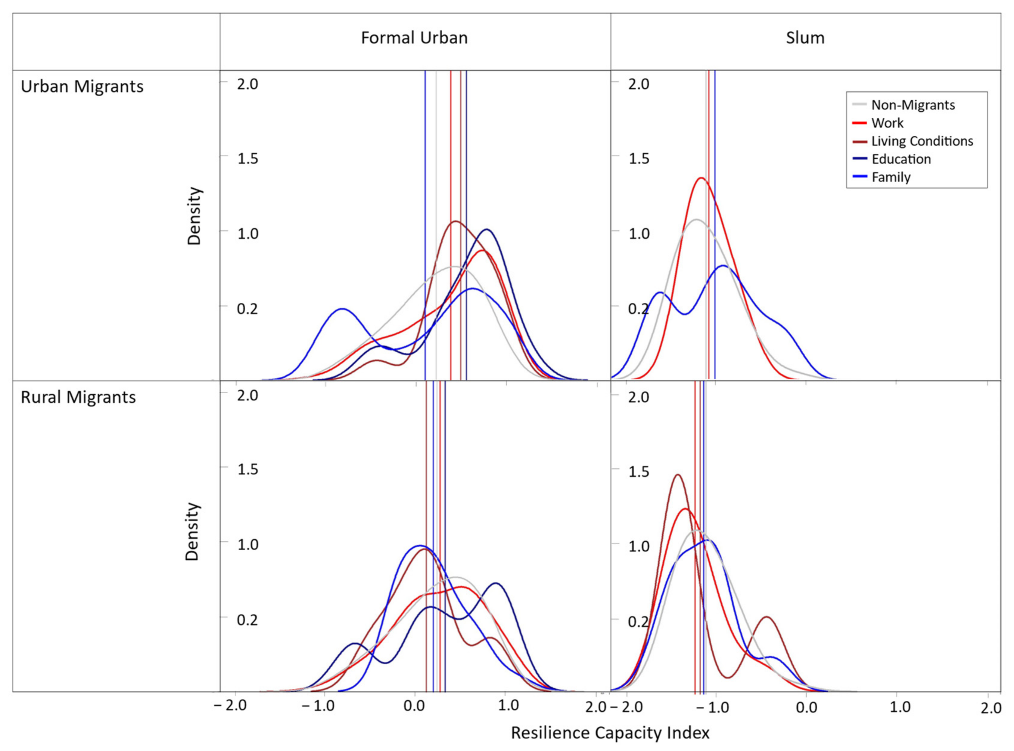
Figure 9.
Resilience matrix displaying kernel density estimation of RCI of sub-groups based on the migration characteristic migration distance.
Figure 9.
Resilience matrix displaying kernel density estimation of RCI of sub-groups based on the migration characteristic migration distance.
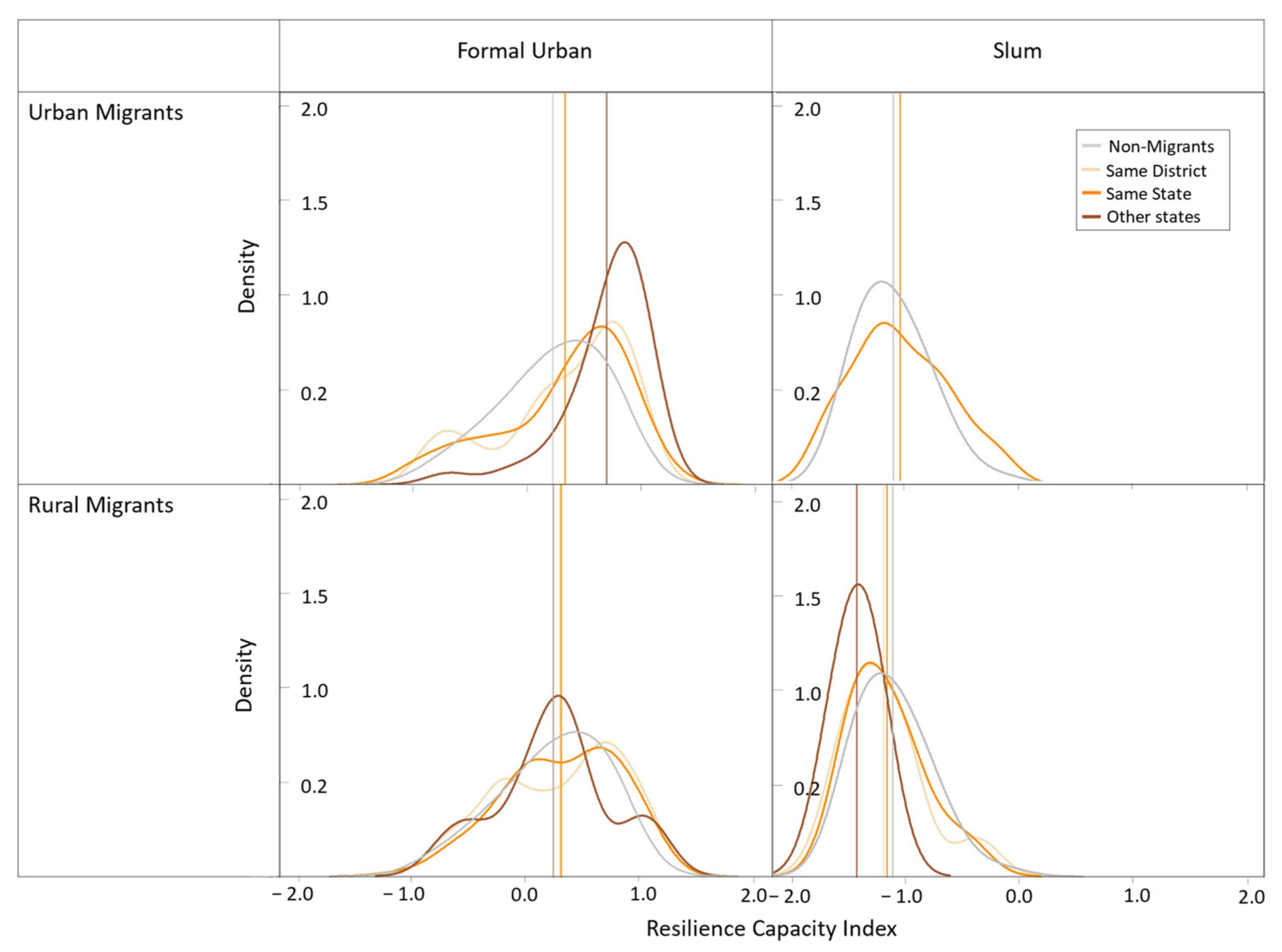
Figure 10.
Resilience matrix displaying kernel density estimation of RCI of sub-groups based on the migration characteristic environmental exposure, displaying flood exposure.
Figure 10.
Resilience matrix displaying kernel density estimation of RCI of sub-groups based on the migration characteristic environmental exposure, displaying flood exposure.
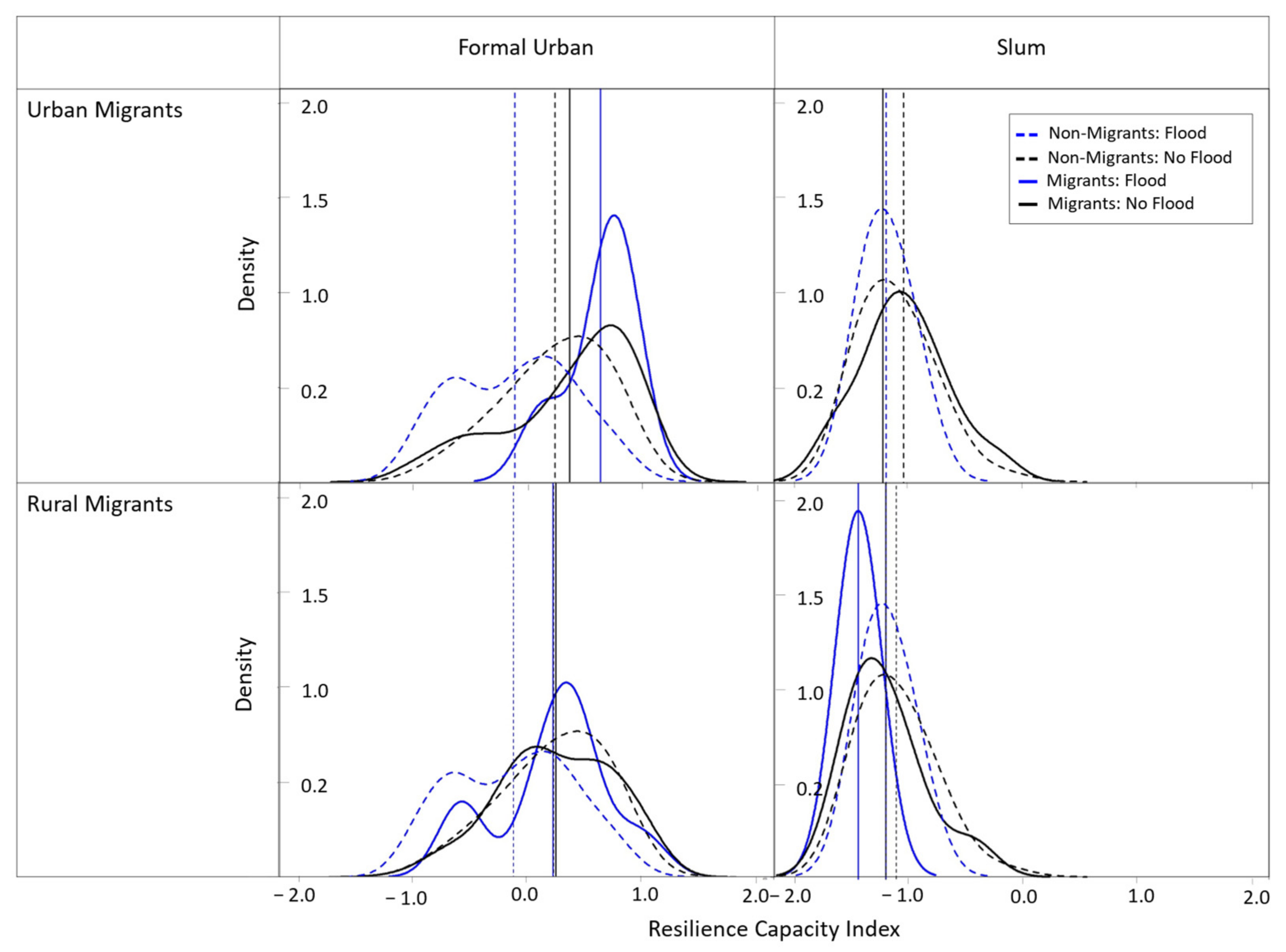
Figure 11.
Resilience matrix displaying kernel density estimation of RCI of sub-groups based on the migration characteristic environmental exposure, displaying heat exposure.
Figure 11.
Resilience matrix displaying kernel density estimation of RCI of sub-groups based on the migration characteristic environmental exposure, displaying heat exposure.

Table 1.
RCI and average object scores of 1st component of each RM pillar for migrants (rural, urban origin) and non-migrants.
Table 1.
RCI and average object scores of 1st component of each RM pillar for migrants (rural, urban origin) and non-migrants.
| Group | RCI | Assets | Housing | Health | n |
|---|---|---|---|---|---|
| Migrants | 0.0562 | 0.0401 | 0.0431 | 0.1458 | 553 |
| Urban | 0.2652 | 0.2849 | 0.3291 | 0.3625 | 193 |
| Rural | −0.0769 | −0.1261 | −0.1988 | 0.1097 | 239 |
| Non-Migrants | −0.0236 | −0.0168 | −0.0181 | −0.0611 | 1319 |
Table 2.
RCI of migrants (urban, rural origin) and non-migrants.
| Group | Formal Urban | n | Slums | n |
|---|---|---|---|---|
| Migrants | 0.2849 | 463 | −1.1205 | 90 |
| Urban | 0.3749 | 178 | −1.0363 | 15 |
| Rural | 0.2568 | 184 | −1.1933 | 55 |
| Non-Migrants | 0.2324 | 1064 | −1.0915 | 255 |
Table 3.
RCI of sub-groups based on the migration characteristic time since arrival (* low sample size).
Table 3.
RCI of sub-groups based on the migration characteristic time since arrival (* low sample size).
| Time SINCE Arrival | Formal Urban | n | Slums | n |
|---|---|---|---|---|
| Non-Migrant | 0.2324 | 1064 | −1.0915 | 255 |
| Urban Migrant | 0.3717 | 178 | −1.0363 | 15 |
| ≤10 | 0.5974 | 75 | −0.6444 | 4 * |
| 10–20 | 0.3138 | 52 | −1.2051 | 9 * |
| >20 | 0.0933 | 50 | NA | 2 * |
| Rural Migrant | 0.2568 | 184 | −1.1933 | 55 |
| ≤10 | 0.3841 | 59 | −0.9845 | 9 * |
| 10–20 | 0.1975 | 69 | −1.1874 | 20 |
| >20 | 0.1957 | 56 | −1.2702 | 26 |
Table 4.
RCI of sub-groups based on the migration characteristic reasons for migration (* low sample size).
Table 4.
RCI of sub-groups based on the migration characteristic reasons for migration (* low sample size).
| Reasons for Migration | Formal Urban | n | Slums | n |
|---|---|---|---|---|
| Non-Migrant | 0.2324 | 1064 | −1.0915 | 255 |
| Urban Migrant | 0.3749 | 178 | −1.0363 | 15 |
| Work | 0.3947 | 98 | −1.0601 | 7 * |
| Living Conditions | 0.5041 | 15 | NA | 0 * |
| Education | 0.5664 | 28 | NA | 1 * |
| Family | 0.1116 | 36 | −0.9935 | 7 * |
| Rural Migrant | 0.2568 | 184 | −1.1933 | 55 |
| Work | 0.2641 | 123 | −1.2148 | 40 |
| Living Conditions | 0.1151 | 11 | −1.1586 | 4 * |
| Education | 0.3228 | 27 | NA | 1 * |
| Family | 0.1927 | 22 | −1.1185 | 9 * |
Table 5.
RCI sub-groups based on the migration characteristic migration distance (* low sample size).
Table 5.
RCI sub-groups based on the migration characteristic migration distance (* low sample size).
| Migration Origin | Formal Urban | n | Slums | n |
|---|---|---|---|---|
| Non-Migrant | 0.2324 | 1064 | −1.0915 | 255 |
| Urban Migrant | 0.4155 | 178 | −1.0434 | 15 |
| Same district | 0.3413 | 16 | NA | 1 * |
| Same state | 0.3403 | 111 | −1.0324 | 11 |
| Other states | 0.7047 | 33 | NA | 2 * |
| Rural Migrant | 0.2957 | 184 | −1.2047 | 55 |
| Same district | 0.2954 | 18 | −1.1715 | 10 |
| Same state | 0.3049 | 113 | −1.1433 | 31 |
| Other states | 0.2353 | 17 | −1.4077 | 11 |
Table 6.
RCI of sub-groups based on the migration characteristic environmental exposure, displaying flood exposure (* low sample size).
Table 6.
RCI of sub-groups based on the migration characteristic environmental exposure, displaying flood exposure (* low sample size).
| Flood Exposure | Formal Urban | n | Slums | n |
|---|---|---|---|---|
| Non-Migrant | 0.2324 | 1064 | −1.0915 | 255 |
| Flood | −0.1109 | 21 | −1.1772 | 7 * |
| No-Flood | 0.2393 | 1043 | −1.0891 | 248 |
| Urban Migrant | 0.3749 | 178 | −1.0363 | 15 |
| Flood | 0.6369 | 5 * | NA | 1 * |
| No-Flood | 0.3673 | 173 | −1.0242 | 14 |
| Rural Migrant | 0.2568 | 184 | −1.1933 | 55 |
| Flood | 0.2333 | 15 | −1.4215 | 3 * |
| No-Flood | 0.2589 | 169 | −1.1801 | 52 |
Table 7.
RCI of sub-groups based on the migration characteristic environmental exposure, displaying heat exposure (night; * low sample size).
Table 7.
RCI of sub-groups based on the migration characteristic environmental exposure, displaying heat exposure (night; * low sample size).
| Heat Exposure (Night) | Formal Urban | n | Slums | n |
|---|---|---|---|---|
| Non-Migrant | 0.2324 | 1064 | −1.0915 | 255 |
| Low | 0.1850 | 451 | −1.0089 | 78 |
| High | 0.2672 | 613 | −1.1279 | 177 |
| Urban Migrant | 0.3749 | 178 | −1.0363 | 15 |
| Low | 0.4357 | 80 | −0.8328 | 5 * |
| High | 0.3253 | 98 | −1.1380 | 10 |
| Rural Migrant | 0.2568 | 184 | −1.1933 | 55 |
| Low | 0.2498 | 105 | −0.9581 | 14 |
| High | 0.2660 | 79 | −1.2736 | 41 |
Publisher’s Note: MDPI stays neutral with regard to jurisdictional claims in published maps and institutional affiliations. |
© 2021 by the authors. Licensee MDPI, Basel, Switzerland. This article is an open access article distributed under the terms and conditions of the Creative Commons Attribution (CC BY) license (https://creativecommons.org/licenses/by/4.0/).
Share and Cite
MDPI and ACS Style
Link, A.-C.; Zhu, Y.; Karutz, R. Quantification of Resilience Considering Different Migration Biographies: A Case Study of Pune, India. Land 2021, 10, 1134. https://doi.org/10.3390/land10111134
AMA Style
Link A-C, Zhu Y, Karutz R. Quantification of Resilience Considering Different Migration Biographies: A Case Study of Pune, India. Land. 2021; 10(11):1134. https://doi.org/10.3390/land10111134
Chicago/Turabian StyleLink, Ann-Christine, Yuanzao Zhu, and Raphael Karutz. 2021. "Quantification of Resilience Considering Different Migration Biographies: A Case Study of Pune, India" Land 10, no. 11: 1134. https://doi.org/10.3390/land10111134
Note that from the first issue of 2016, this journal uses article numbers instead of page numbers. See further details here.