Influence of Aspect and Elevational Gradient on Vegetation Pattern, Tree Characteristics and Ecosystem Carbon Density in Northwestern Himalayas

Abstract

Himalayan forest has been threatened by rapid anthropogenic activities, resulting in the loss of forest diversity and climate change. The present study was carried out on four aspects (northern, southern, western and eastern), at three different altitudinal ranges, namely, 1000–1300 m above sea level (m a.s.l.), 1300–1600 m a.s.l. and 1600–1900 m a.s.l., and at three diverse mountain ranges (Kalaghat, Barog and Nangali) of sub-temperate forest ecosystems of the mid Himalayan ranges, to elucidate their influence on vegetation, tree characteristics and ecosystem carbon density. The results revealed that Pinus roxburghii is the most dominant forest community of the mid Himalaya’s forest, irrespective of altitudinal gradient and slope. The south-facing slopes are occupied by the xerophytic tree species frequently found in the lower Shiwalik P. roxburghii forest, whereas the north-facing ones are dominated by mesophyllic species, such as Cedrus deodara and Quercus leucotrichophora, which commonly grows in the northwestern Himalayan temperate forest ecosystem. The maximum stem density (211.00 Nha⁻¹) was found at 1000–1300 m a.s.l., and on the northern aspect (211.00 Nha⁻¹). The maximum stem volume (236.50 m³ ha⁻¹) was observed on the northern aspect at 1000–1300 m a.s.l., whereas the minimum (32.167 m³ ha⁻¹) in the southern aspect at 1300–1600 m a.s.l. The maximum carbon density (149.90 Mg ha⁻¹) was found on the northern aspect and declined with increasing elevation from 123.20 to 74.78 Mg ha⁻¹. Overall, the study establishes that the southern and western aspects are very low in carbon density, whereas the northern aspect represents higher biodiversity as well as carbon and nutrient stocks. Therefore, aspect and altitude should be given due importance for efficient managing of biodiversity and mitigating climate change.

1. Introduction

In recent decades, Himalayan forest has been threatened by rapid anthropogenic activities, resulting in the loss of forest diversity and climate change. Mountain forests cover about 23% of the total forest land area [1] and host ~12% of the human population worldwide [2]. Compared to other mountain ecosystems, the Indian Himalayan region is dynamically young [3] and harbors a wide variety of biodiversity apart from sustaining life for a significant part of the Indian subcontinent population. Vegetation cover plays a crucial role in local, regional and global climate apart from decreasing erosion in mountain areas [4]. By adopting sustainable environmental management practices, the protection of mountainous habitats (particularly, biological diversity) will help in safeguarding livelihoods and further improvement of local communities. They also shield individuals effectively from natural calamities, e.g., debris flows, floods and landslides [5]. In forest conservation and management, tree diversity plays an important role because it provides resources and shelter to forest species [6]. Besides its effect on species diversity and ecosystem functioning, it also affects tolerance and resistance to climate changes in the future [7,8]. Several edaphic factors and topographical factors (e.g., altitude, aspect and slope) control vegetation growth [9,10] and play a vital role in plant species distribution [7,11]. Altitude plays a key role in deciding the temperature system and diversification of forest species [12,13]. Moreover, co-factors such as soil type and slope propensity help in guiding forest composition at one altitude [14,15]. The determinants of species richness are altitude, physiography, productivity [16] and biotic variables. A comprehension of stand characteristics and forest structure is a prerequisite for identifying different ecological processes and modeling the functioning and dynamics of forests [17]. Several biotic (e.g., intensity of photosynthesis, leaf area index, forest types and plant architecture) and abiotic characteristics (e.g., solar radiation, temperature, soil moisture and length of growing season) affect carbon cycling and further affect the regional and/or global carbon budget [18,19,20,21].

In addition to being a crucial natural constraint to climate change, forest habitats occupy approximately 30% of land areas and play a dominant role in the exchange of carbon dioxide (CO₂) between the atmosphere and biosphere [22,23]. Major shares (81%) of the terrestrial carbon (C) biomass are found in forest ecosystem [24], where 2/3 of the C is fixed annually in terrestrial ecosystems [25]. Vegetation biomass is a central ecological element to understand the climate system’s evolution and possible future changes. Therefore, biomass acts as an important indicator of climate change prediction models, and further helps to make mitigation and adaptation strategies [26]. Forests, particularly primary ones, are actively engaged in the cycling of carbon (i.e., C stock in vegetation and its underlain soil through the process of photosynthesis and respiration) [27], and the extent depends on age, tree species, location of forests and management practices [28]. Due to land-use change and tropical deforestation, nearly 1.7 billion tons of carbon is emitted annually, which impacts climate badly [29,30]. The tree biomass pool is a vital origin of uncertainty in C balance in tropical regions [31] and plays a crucial role in the global C cycle. The management of forests for maintaining or enhancing carbon stocks is receiving increasing interest from forest land owners and land management agencies [32,33] due to the impacts from a change in climate intensity [34].

The structure and functions of Himalayan forests are believed to be changing over time, resulting in loss of forest diversity [35]. In most of the studies, the parameters pertaining to forest productiveness are overestimated because of the unaccountability of slope and aspects [36]. The ecological studies and biomass estimation along altitudinal gradients in forests of western Himalaya have been well documented over the years [37,38,39]. However, the literature reveals that very few studies report the effect of aspect in the northwestern Himalayas on forest ecosystems. For the effective management of forest ecosystems in the mid-hill of the Himalayas, there is an urgent need to know the key indicators that impact the tree characteristics, plant communities, forest biomass and its underlying soil with respect to elevation gradients, slope and aspect [7,36,40]. The objectives of our study were to test the hypothesis that different aspects (northern, eastern, western and southern) and altitudinal ranges influence the tree characteristics, vegetation biomass, total carbon stocks and physico-chemical characteristics of the soil. By taking into consideration these objectives, we shall be able to answer these above issues for the management and conservation prospective of forest ecosystems in the mid hills of the Himalayas. This study would be helpful in designing afforestation and reforestation programs for different altitudes and aspects in the mid Himalayas, for enhanced carbon sequestration and mitigating climate change.

2. Materials and Methods

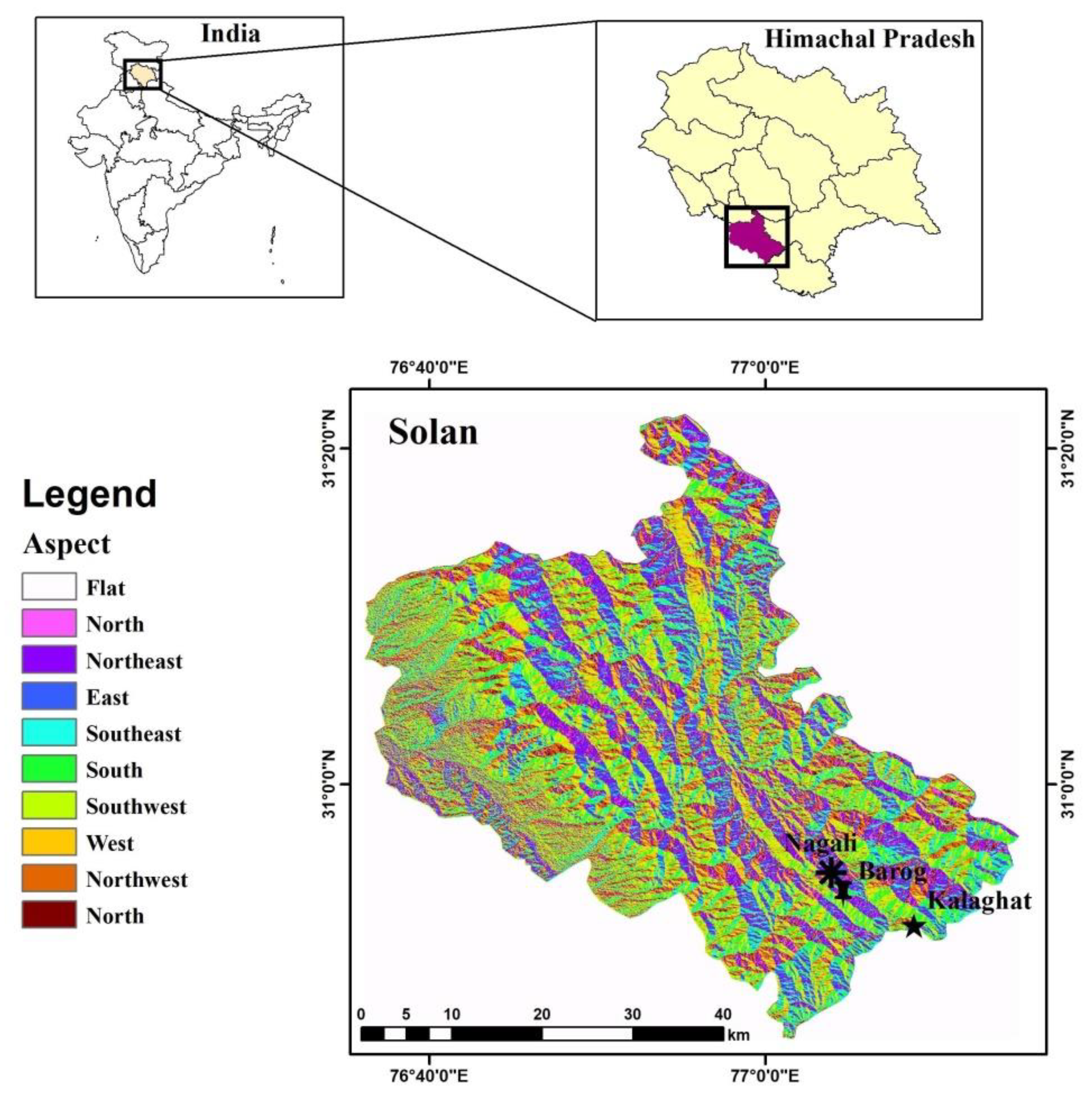
2.1. Study Area

The present study was carried out at three altitudinal ranges: AR₁ (1000–1300 m above mean sea level (m a.s.l.)), AR₂ (1300–1600 m a.s.l.) and AR₃ (1600–1900 m a.s.l.); at four aspects: northern (N), southern (S), eastern (E) and western (W); and at three separate mountainous ranges (Kalaghat, Barog and Nangali) located in the Solan district of Himachal Pradesh (H.P), India, situated in the middle of the NW Himalayas. The area lies between 30°51′16′′ to 30°53′40′′ N latitudes and 77°9′27′′ to 77°3′51′′ E longitude (Survey of India Toposheet No. 53F/1) and lies in a transitional zone between the sub-tropical to moist temperate Himalayas and falls under the Champion and Seth forest type of lower Shiwalik P. roxburghii forest (9/C_1a), Upper Himalayan P. roxburghii forest (9/C_1b) and Lower western Himalayan temperate forest (12/C₁). The seasons are well marked, and there are distinct pre-monsoon, monsoon, post-monsoon and winter seasons. On average, the annual rainfall ranges from 1000 to 1400 mm, with little pre-monsoon precipitation, and July–September contribute the most to precipitation. Winter precipitation of low quantum is common. The mean minimum and maximum temperatures differ between 1 °C in the winter and 35 °C in the summer with a mean annual temperature (MAT) of 20 °C. The parent material is composed of shale, schist, quartzite and slate, with a sandy loam to loam and clayey texture in discrete pockets. Brown and podzol soil forms commonly occur in the upper regions. The soils are rich in nutrients and organic matter (OM) except sites that are too exposed and eroded.

2.2. Vegetation Sampling and Data Analysis

During the winter season of 2017, a reconnaissance survey of the region was carried out to identify the mountain ranges for the present investigation (Figure 1). In this study area, the three altitudinal ranges, AR₁, AR₂ and AR₃, of the three separate mountainous (Kalaghat, Barog and Nagali) regions were selected. At every altitude, the four aspects, i.e., the N-, S-, W- and E-facing slopes, each had three sample plots of 0.1 ha (31.62 m × 31.62 m),which were randomly laid out on the surveyed area to analyze the tree composition (12 elevation stands × 3 sample plot each with a total of 36 sample plots). For the shrub- and herb-related characteristics, four subplots of size 5 m × 5 m and eight plots of 1 m × 1 m were laid out within each tree sample plot, respectively. Further, the density of the trees was determined by counting trees in each sample plot. In each sample plot, trees and shrubs were marked and counted to determine the community parameters viz. the frequency, stand density and Importance Value Index (IVI) [41]. The forest associations and forest types were named based on tree composition and their stand density values. The identification of plants was done with the help of the Herbarium of Dr. YSP University of Horticulture and Forestry, Nauni, Solan, and the current taxonomic literature. Tree height was measured using a Ravi multimeter (BlumeLeiss Hypsometer) from the uphill side in the slopy areas [42], whereas the diameter of trees was measured at breast height (DBH, about 1.37 m). The diameter of the grasses, herbs, shrubs and regeneration were derived from the girth measured at the collar portion. Crown height (m) was taken from the ground level to the point halfway between the lowest green branch and the green branches forming a green crown all around. Similarly, crown length (m) was the vertical length from the top to the point halfway between the lowest green branch and the green branches forming a green crown all around. The diameter of the crown was determined in two directions (N–S and E–W) and the mean diameter was estimated as per Assmann [43] and Chaturvedi and Khanna [42].

2.3. Biomass and Carbon

The allometric equations proposed by the Forest Survey of India (FSI) and Forest Research Institute (FRI) for respective forest tree species were used to estimate the growing stock volume density (GSVD; m³ ha⁻¹) [44]. After that, the estimated GSVD of the individual tree species was converted into total tree biomass as the Above Ground Biomass Density (AGBD; Mg ha⁻¹) by multiplying the GSVD of the tree species by the Biomass Expansion Factor (BEF) expressed below [45]. Specific gravity (SG) was calculated by the method adopted by Rajput et al. [46].

Stem biomass (SB) = Average SG wood × Volume

(1)

The BEF for hardwood is expressed by BEF = exp {1.91–0.34 × ln (GSVD)} (for GSVD ≤ 200 m³ ha⁻¹), but in the case of pine species, it is used as a fixed value based on the GSVD (i.e., BEF for GSVD < 10, 10–100 and >100 m³ ha⁻¹ are used as 1.68, 0.95 and 0.81 respectively) [47].

AGBD = GSVD × BEF

(2)

The tree volume could be transformed into biomass by multiplying it with specific gravity using the maximum moisture method [48]. Belowground biomass density (BGBD) of trees was calculated by following IPCC [49] guidelines [22,50]. Further, total biomass of the tree was finally computed by adding AGB and BGB. Moreover, the biomass of the herbs and shrubs were calculated by the oven-dried weight. Thus, each shrub and herb sample collected were brought to the laboratory followed by segregation into leaves, branches and a stem portion after washing and oven-dried at 70 °C for 72 h till a constant dry weight was achieved. Each sample was weighed to estimate AGB (including the stem, branch and leaves) of each species. BGB is estimated by extracting the roots of the sample plant (shrubs). The extract of the root sample was packaged in the paper and brought to the laboratory to know the biomass. First of all, root hairs of individual species were washed thoroughly and weighed to know their fresh weight (Wi) and after that dried at 70 ± 5 °C for 72 h to estimate their dry weight. Similarly, total biomass of a shrub species was calculated by adding its AGB and BGB components.

2.4. Total Carbon Density

Total carbon density (or stocks) of forest vegetation was estimated by vegetation biomass (AGB+BGB) multiplied by a default value of 0.50 [49].

2.5. Vegetation Carbon Density

Vegetation carbon density (VCD) was calculated by adding all the biomass (tree, shrubs and herbs).

VCD = Tree biomass + Herb biomass + Shrub Biomass

(3)

2.6. Determination of Soil Characteristics

The soil samples were taken from the soil profile at 0–20 cm and 20–40 cm depths in three replications from each 0.1 ha sample plot. These samples were then sun-dried and sieved to a 2-mm size. The soil pH was determined by a combined glass–calomel electrode of aqueous suspensions (1:2.5 soil:water ratio). Electrical conductivity (dS m⁻¹) was estimated by a conductivity bridge [51] of aqueous suspensions (1:2 soil:water ratio). Soil organic carbon (SOC) was estimated by a well-known method of wet digestion [22,52]. Potassium (K) was measured by a flame photometer [53] and available nitrogen (N) and phosphorus (P) by the alkaline permanganate method [54].

2.7. Ecosystem Carbon Density

The total ecosystem carbon density (ECD) is referred to as the sum of all carbon pools, including the soil carbon density or stocks, and was measured as

ECD = SOC + Detritus carbon density + Tree carbon density

(4)

Soil carbon density was calculated as follows: Soil bulk density (g cm⁻³) × Depth of soil (cm) × Carbon (%) [55]. Solar radiation was estimated using a Lux meter.

2.8. Statistical Analysis

In this study, the data obtained on variations in vegetation, tree characteristics and ecosystem carbon density were subject to statistical analysis by Factorial Randomized Block Design using R Studio data analysis software, as follows:

Package: doebioresource

Function: frbd2fact

Syntax: frbd2fact (data, replicationvector, fact.A, fact.B, Multiple.comparison.test)

Arguments:

Data: dependent variables; Replication vector: vector containing replications; fact.A: vector containing levels of first factor; fact.B: vector containing levels of second factor; Multiple.comparison.test: 0 for no test, 1 for lsd test, 2 for Duncan test and 3 for HSD test

The significance of the effect of aspect and altitudinal ranges on different parameters was judged using an LSD post-hoc test.

3. Results

3.1. Floristic Composition of Vegetation Species

The distribution of the floristic composition of the tree species growing at the study sites varied with altitudinal range (Table S1). Among the tree species, Pinus roxburghii was dominant followed by Quercus leucotrichophora and Erythrina indica. At the 1000–1300 m a.s.l. altitudinal range (AR₁), the maximum number of tree species (4) was recorded on the northern aspect followed by the eastern, southern and western slopes, respectively. At the 1300–1600 m a.s.l. (AR₂) altitudinal range, the maximum number of species (6) was recorded on the southern (S) aspect followed by the eastern (E) and northern (N) ones, respectively. However, at the 1600–1900 m a.s.l. altitudinal range (AR₃), the maximum number of species (3) were recorded on the northern aspect followed by the western aspect. Among the three altitudinal ranges, the AR₂ altitude range displayed the highest number of tree species, i.e., 14, while the lowest number was at AR₃ (7). Similarly, 21 shrub species represent the mid-hills of the northwestern Himalayas, out of which the prominent species are Berberis aristata, Carissa carandas and Lantana camara, etc., whereas Cassia floribunda, Hypericum oblongifolium and Sarcocoas aligna are the least prominent ones (Table S2). At the AR₁ altitudinal range, the maximum numbers of shrub species were found on the southern aspect followed by the western, northern and eastern aspects, respectively. At the AR₂ altitudinal range, the northern and southern aspects were represented by 7 species of shrubs, whereas the eastern and western aspects were represented by six species each. At the AR₃ altitudinal ranges, the number of species on the western and southern aspects were slightly more than the eastern and northern aspects. In general, the number of shrub species declined with increasing altitudinal ranges.

The overall status of plant diversity composition is presented in Figure S1. It reveals that the mid-hills of the northwestern Himalayas are richer in shrub diversity than the trees as measured by family, genus and species presence. Maximum diversity in trees and shrubs was measured on the S-facing slope at 1300–1600 m a.s.l. and 1000–1300 m a.s.l., respectively. Maximum biodiversity was found on the S-facing slope, followed by north, east and west, respectively.

3.2. Distribution of Vegetation Communities and Forest Types

The floristic composition concerning vegetation communities and forest type identified revealed that P. roxburghii is an important component of all the communities at all the combinations of altitude and aspect (Table S3). Lower (1000–1300 m a.s.l.) and upper (1600–1900 m a.s.l.) altitudinal ranges of the E- and W-facing slopes of the study area were represented by the P. roxburghii community, whereas the mid-altitude (1300–1600 m a.s.l.) by the P. roxburghii–Quercus leucotrichophora and P. roxburghii–Myrica esculenta community, respectively. The N-facing slopes are represented by the P. roxburghii–Q. leucotrichophora community at all the altitudinal gradients. However, the S-facing slopes are represented by the P. roxburghii–A. catechu community at a low altitude; P. roxburghii, Acacia catechu and a diverse mixture of broad-leaved vegetation at mid altitude; and a pure P. roxburghii community at a higher altitude. The vegetation of the E- and W-facing slopes is classified into Himalayan subtropical pine forest (9/C₁), subtype Upper Himalayan P. roxburghii forest (9/C_1b). S-facing slopes belong to the same forest type but a different subtype, i.e., Lower Shiwalik P. roxburghii forest (9/C_1a). However, the N-facing slopes belong to entirely different forest types, i.e., Lower western Himalayan temperate Ban Q. leucotrichophora forest (12 C₁).

3.3. Variation in Tree Characteristics

The various tree characteristics, namely, DBH, height, crown length, stem density, stem volume and stem biomass, of the studied forest ecosystems are depicted in

Table 1. Tree parameters and biomass density on the different aspects and altitudinal ranges.

Altitudinal Ranges (AR) (m a.s.l.)	Aspect (A)
	E	W	N	S	Mean
DBH (cm)
AR1 (1000–1300)	25.00	19.00	36.30	23.40	26.00 a
AR2 (1000–1300)	22.00	18.60	22.50	22.80	22.00 b
AR3 (1000–1300)	26.20	20.00	26.00	19.40	20.00 b
Mean	28.00 a	21.80 b	22.00 b	21.16 b
LSD	AR = 3.70		A = 4.30	AR × A = 3.90
Height (m)
AR1 (1000–1300)	14.50	10.22	22.40	16.48	16.26 a
AR2 (1000–1300)	13.00	9.30	11.60	10.00	12.18 b
AR3 (1000–1300)	12.00	12.30	13.00	10.00	11.38 b
Mean	13.90 ab	12.40 bc	16.30 a	10.50 c
LSD	AR = 2.70		A = 3.20	AR × A = NS
Crown length (m)
AR1 (1000–1300)	4.70	5.50	7.90	4.40	6.00 a
AR2 (1000–1300)	6.00	4.60	5.30	3.50	5.00 a
AR3 (1000–1300)	5.00	3.00	3.15	2.20	3.00 b
Mean	5.16	3.70	5.20	4.40
LSD	AR = 1.90		A = NS	AR × A = 4.50
Stem density (N ha−1)
AR1 (1000–1300)	258.00	198.00	217.00	170.00	211.00 a
AR2 (1000–1300)	228.00	175.00	283.00	165.00	188.00 a
AR3 (1000–1300)	116.00	188.00	133.00	143.00	146.00 b
Mean	200.00 ab	154.60 c	211.00 a	166.00 bc
LSD	AR = 37.00		A = 43.00	AR × A = NS
Stem volume (m3 ha−1)
AR1 (1000–1300)	118.83	40.90	236.50	74.40	117.68 a
AR2 (1000–1300)	132.16	39.50	105.40	32.17	77.33 b
AR3 (1000–1300)	101.58	35.30	40.90	53.00	57.89 b
Mean	127.60 a	53.00 b	117.50 a	38.60 b
LSD	AR = 38.80		A = 44.80	AR × A = 53.23
Stem biomass (Mg ha−1)
AR1 (1000–1300)	120.50	36.58	72.75	21.58	82.85
AR2 (1000–1300)	58.92	16.25	132.16	18.66	56.50
AR3 (1000–1300)	20.08	35.50	63.91	21.91	35.35
Mean	66.50 a	29.44 b	89.61 a	20.72 b
LSD	AR = NS		A = 30.73	AR × A = 53.23

E—Eastern, W—Western, N—Northern, S—Southern, NS—non-significant. Mean values in the same column followed by a different letter differ significantly at p ≤ 0.05 according to lsd post-hoc test.

.

3.3.1. Diameter at Breast Height (DBH, cm)

The maximum average DBH of 26.00 cm was recorded at AR₁, which was found to be significantly (p < 0.05) higher than both AR₂ and AR₃ (Table 1). Irrespective of altitudinal ranges, maximum DBH was recorded on the eastern aspect and was significantly higher (p < 0.05) than the other aspects. The order of DBH among different aspect followed the following trend: eastern (28.00 cm) > northern (22.00 cm) > southern (21.16 cm) > western (21.00 cm). In the interaction, the maximum DBH (36.30 cm) was recorded on the northern aspect at AR₁, whereas the minimum (18.60 cm) was found on the western aspect at AR₂.

3.3.2. Height (m)

Height (Table 1) showed a declining trend with an increase in altitude. AR₁ displayed a significant difference (p < 0.05) over both AR₂ and AR₃. Among the studied aspects, the N-facing slopes demonstrated superiority over the other aspects. In the interaction, an inconsistent trend was observed at the aspect level with an increase in altitudinal range. The maximum (22.40 m) height growth was noticed on the northern aspect at AR₁ and the minimum (9.30 m) was on the western aspect (AR₂).

3.3.3. Crown Length (m)

It is evident from Table 1 that among the altitudinal ranges, the maximum crown length (6.00 m) was recorded at AR₁ and was significantly higher (p < 0.05) than AR₃, only. The maximum crown length (5.20 m) was recorded on the northern aspect and minimum (3.70 m) on the western aspect. The maximum crown length (7.90 m) in the interaction was seen on the northern aspect at AR₁, whereas the minimum (2.20 m) was on the northern aspect at AR₃.

3.3.4. Stem Density (N ha⁻¹)

Stem density (N ha⁻¹) was found to be significantly influenced by altitudinal variation and aspect (Table 1). It declined with increasing altitude, and both AR₁ and AR₂ evinced markedly higher values over AR₃. Stem density was found to be maximum (211.00 Nha⁻¹) on the northern aspect, which was statistically at par with eastern aspect. However, interaction effect between the altitude and aspect could not exercise a significant influence on the stem density.

3.3.5. Stem Volume (m³ ha⁻¹)

Stem volume (m³ ha⁻¹) was also significantly influenced by altitude, aspect (Table 1), and it declined with the increase in the altitude. A significant influence was observed between AR₁ over AR₂ and AR₃. Irrespective of altitudinal gradients, maximum stem volume (127.60 m³ ha⁻¹) was recorded on eastern aspect but was significantly at par with the northern aspect. Minimum stem volume (38.60 m³ ha⁻¹) was recorded on the southern aspect, however it remains at par with western one. In the interaction, maximum stem volume (236.50 m³ ha⁻¹) was recorded on northern aspect at AR₁, whereas minimum stem volume (32.17 m³ ha⁻¹) was recorded on southern aspect at AR₂.

3.4. Vegetation Biomass and Carbon Density

3.4.1. Above Ground-Below Ground Biomass (Mg ha⁻¹)

Table 2. Vegetation biomass and carbon density at different aspects and altitudinal ranges.

Altitudinal Ranges (AR) (m a.s.l.)	Aspect (A)
	E	W	N	S	Mean
Above ground biomass (t ha−1)
AR1 (1000–1300)	222.05	69.88	130.61	42.49	116.25 a
AR2 (1000–1300)	112.44	31.14	252.31	43.36	109.81 a
AR3 (1000–1300)	38.38	67.87	115.75	33.07	63.76 b
Mean	124.28 a	56.29 b	166.22 a	39.64 b
lsd	AR = 40.00		A = 55.25	AR × A = 95.693
Below ground biomass (t ha−1)
AR1 (1000–1300)	47.88	14.67	41.65	9.39	28.40
AR2 (1000–1300)	29.77	6.54	90.31	7.6	33.56
AR3 (1000–1300)	8.06	22.96	32.24	6.94	17.5
Mean	28.57 b	14.72 bc	54.73 a	7.98 c
lsd	AR = NS		A = 18.74	AR × A = 32.46
Total tree biomass (t ha−1)
AR1 (1000–1300)	315.65	84.56	172.26	51.88	156.08 a
AR2 (1000–1300)	142.21	37.68	342.62	53.09	143.90 a
AR3 (1000–1300)	46.44	90.83	147.99	40.01	81.32 b
Mean	168.09 a	71.02 b	220.95 a	48.32 b
lsd	AR = 58.69		A = 67.77	AR × A = 117.388
Shrub biomass (Mg ha−1)
AR1 (1000–1300)	1.84	1.75	1.85	2.37	1.95 a
AR2 (1000–1300)	1.60	1.76	1.56	1.79	1.67 ab
AR3 (1000–1300)	1.40	1.33	1.38	1.72	1.45 b
Mean	1.61	1.62	1.59	1.96
lsd	AR = 0.303		A = NS	AR × A = NS
Herb biomass (Mg ha−1)
AR1 (1000–1300)	2.93	3.27	3.10	3.92	3.30
AR2 (1000–1300)	3.24	2.77	2.80	3.94	3.19
AR3 (1000–1300)	2.55	2.46	2.22	3.49	2.68
Mean	2.90 b	2.83 b	2.71 b	3.78 a
lsd	AR = NS		A = 0.63	AR × A = NS
Vegetation biomass density (Mg ha−1)
AR1 (1000–1300)	320.41	89.57	177.22	57.97	161.29 a
AR2 (1000–1300)	146.82	42.11	347.33	58.66	148.73 a
AR3 (1000–1300)	50.39	94.63	151.86	45.16	85.50 b
Mean	172.62 a	75.46 b	225.27 a	53.93 b
lsd	AR = 58.78		A = 67.85	AR × A = 117.52

E—eastern, W—western, N—northern, S—southern, NS—non-significant. Mean values in the same column followed by a different letter differ significantly at p ≤ 0.05 according to the LSD post-hoc test.

evinced that significantly maximum AGB (116.25 Mg ha⁻¹) was recorded at AR₁. Among the aspects, the maximum AGB (166.22 Mg ha⁻¹) was recorded on the northern aspect and the minimum (39.64 Mg ha⁻¹) on southern ones. The trend observed for AGB on different aspects followed the order: N > E > W > S. In the interaction between the aspect and altitudinal ranges, northern aspect displayed maximum biomass accumulation (252.31 Mg ha⁻¹) at 1000–1600 m a.s.l. range, and was found to be considerably higher than others. The results in respect of BGB and total biomass for altitudinal gradient, aspects, and their interaction followed more or less similar trend as that of AGB.

3.4.2. Shrub and Herb Biomass (Mg ha⁻¹)

Table 2 shows that shrub biomass was significantly influenced by altitudinal ranges, whereas herb biomass significantly differed between aspects. This shrub biomass decreased with an increase in altitude (highest at AR₁: 1.95 Mg ha⁻¹ and lowest at AR₃: 1.45 Mg ha⁻¹). Among the different aspects, the maximum shrub biomass (1.96 Mg ha⁻¹) was estimated on southern aspect and the minimum (1.59 Mg ha⁻¹) on the northern ones. Similarly, the maximum biomass of herbs (2.90 Mg ha⁻¹) was recorded on the eastern aspect, and the minimum (2.71 Mg ha⁻¹) on northern.

3.4.3. Vegetation Biomass Density (Mg ha⁻¹)

Vegetation biomass density declined with an increase in elevation; however, significant differences (p < 0.05) were seen between AR₁ and AR₃ (Table 2). Vegetation biomass (225.27 Mg ha⁻¹) was maximum on the northern aspect followed by eastern, western and southern, respectively. The interaction between altitudinal gradient and aspect also exercised a significant influence on the vegetation biomass density. On the eastern, western and southern aspects, the maximum values for this parameter were at AR₁; however, on the northern aspects, the maximum vegetation biomass density (347.32 Mg ha⁻¹) was at the altitudinal range of 1600–1900 m a.s.l.

Vegetation, soil and total ecosystem carbon density declined with the increase in altitudinal range. However, significant differences were seen between AR₁ and AR₃ (

Table 3. Carbon density in different pools, ecosystem carbon density and solar radiation at different aspects and altitudinal ranges.

Altitudinal Ranges (AR) (m a.s.l.)	Aspect (A)
	E	W	N	S	Mean
Vegetation carbon density (Mg ha−1)
AR1 (1000–1300)	160.21	44.79	88.61	28.98	80.64 a
AR2 (1000–1300)	73.41	21.05	173.67	29.33	74.36 ab
AR3 (1000–1300)	25.20	47.31	75.93	22.58	42.75 b
Mean	86.27 a	37.71 b	112.73 a	26.96 b
LSD	AR = 33.92		A = 29.38	AR × A = 58.76
Soil carbon density (Mg ha−1)
AR1 (1000–1300)	43.23	40.83	33.83	39.77	39.42 a
AR2 (1000–1300)	40.93	36.90	36.67	37.50	38.00 a
AR3 (1000–1300)	25.53	28.20	31.43	29.40	28.64 b
Mean	36.56	35.31	33.97	35.55
LSD	AR = 36.56		A = NS	AR × A = 5.94
Soil humus carbon density (Mg ha−1)
AR1 (1000–1300)	1.57	0.73	1.23	1.60	1.28 b
AR2 (1000–1300)	3.10	1.33	1.73	2.57	2.18 a
AR3 (1000–1300)	2.17	1.27	1.17	1.80	1.60 b
Mean	2.28 a	1.11 c	1.38 bc	1.99 ab
LSD	AR = 0.55		A = 0.64	AR × A = NS
Leaf litter carbon (Mg ha−1)
AR1 (1000–1300)	2.22	2.02	1.25	1.92	1.85 b
AR2 (1000–1300)	2.17	1.94	2.06	2.11	2.07 a
AR3 (1000–1300)	1.98	1.78	1.71	1.95	1.86 b
Mean	2.12 a	1.91 c	1.67 d	1.99 a
LSD	AR = 0.02		A = 0.051	AR × A = 0.11
Ecosystem carbon density (Mg ha−1)
AR1 (1000–1300)	207.23	88.37	125.73	71.58	123.20 a
AR2 (1000–1300)	119.61	61.22	214.13	70.66	116.40 a
AR3 (1000–1300)	54.88	78.56	110.52	55.20	74.78 b
Mean	127.20 a	76.11 b	149.90 a	65.80 b
LSD	AR = 29.60		A = 34.18	AR × A = 59.21

E—eastern, W—western, N—northern, S—southern, NS—non-significant. Mean values in the same column followed by a different letter differ significantly at p ≤ 0.05 according to the LSD post-hoc test.

). Carbon stored in the form of humus was maximum at AR₂, while the carbon stored in the leaf litter increased significantly with rising altitude. Among the four aspects, VCD and ECD were significantly (p < 0.05) at their maximum on the northern aspects.

In contrast, carbon stored in the form of humus was significantly higher (p < 0.05) on the eastern aspect and followed the following trend: E > S > N > W. Interaction between altitudinal gradient and aspects also exercised a significant influence on the carbon density of different pools, except the humus. On the eastern aspects, the maximum values for the vegetation carbon pool were at AR₁; however, on the northern aspects, the maximum vegetation biomass was at the AR₂ altitudinal range. Soil carbon density also varied significantly (p < 0.05) at different altitudes with aspects. In general, the values on the different aspects declined with an increase in altitude. Carbon density stored in the leaf litter on the eastern and western aspects declined rapidly with an increase in altitude from AR₁ to AR₃. On the northern and southern aspects, the maximum value was observed at AR₂. The maximum ECD (214.13 Mg ha⁻¹) was recorded on the northern aspect, which remained statistically identical to AR₁ of the eastern aspect. The ECD did not vary significantly (p < 0.05) at the western and southern aspects with the variation in altitudinal range.

3.5. Soil Physico-Chemical Characteristics

The soil physico-chemical characteristics of the sites under investigation is depicted in

Table 4. Soil physico-chemical characteristics in different aspects and altitudinal ranges.

Treatment	Parameters
	pH	Bulk Density (g cm−3)	Organic Carbon (g kg−1)	Available N (kg ha−1)	Available P (kg ha−1)	Available K (kg ha−1)	EC (dS m−2)
Altitudinal range (AR) (m a.s.l.)
AR1 (1000–1300 m a.s.l.)	6.09 b	0.86 c	22.8 a	413.22 a	19.78 a	242.37 a	0.31 a
AR2 (1300–1600 m a.s.l.)	6.31 a	0.90 bc	21.2 b	355.68 b	16.70 b	223.38 b	0.30 b
AR3 (1600–1900 m a.s.l.)	5.98 c	0.94 a	15.3 c	327.11 c	13.42 c	209.20 c	0.29 c
LSD (E)	0.09	0.051	0. 89	21.23	1.33	6.87	0.009
Aspect (A)
E (Eastern)	5.98 c	0.87 bc	19.9 b	347.28 b	15.87 b	229.63 a	0.29 b
W (Western)	5.99 c	0.92 ab	19.3 bc	330.86 c	18.43 a	213.54 b	0.29 b
N (Northern)	6.18 b	0.85 c	21.2 a	480.80 a	18.62 a	195.79 c	0.31 a
S (Southern)	6.34 a	0.96 a	18.6 c	304.39 d	13.60 c	200.98 c	0.30 ab
LSD (A)	0.11	0.059	1.03	24.51	1.54	7.93	0.01
Soil layers (cm)
L1 (0–20 cm)	5.95 b	0.79 a	21.0 a	380.19 a	18.25 a	235.89 a	0.31
L2 (20–40 cm)	6.30 a	1.01 b	18.5 b	350.48 b	15.01 b	214.08 b	0.30
LSD (L)	0.07	0.04	0. 73	17.33	1.09	5.61	NS

* EC = electric conductivity. Mean values in the same column followed by a different letter differ significantly at p ≤ 0.05 according to the LSD post-hoc test.

. pH value (6.31) was found significantly (p < 0.05) higher at AR₂ (1300–1600 m a.s.l.) than both AR₁ and AR₃. Among the aspects, the maximum pH (6.34) was recorded on the southern aspect and followed the following trend: southern > northern > western > eastern. The organic carbon (OC) and available nutrients (particularly, N, P and K), declined significantly (p < 0.05) with the increasing altitudinal ranges.

OC, available N and P were found to be highest on the northern aspect and lowest on the southern aspect, whereas available K was the highest on the eastern aspect. Bulk density showed an increasing trend with elevational range. Bulk density was maximum (0.96 g cm³) on the southern aspect, followed by western, eastern and northern, respectively. The values of the pH and bulk density increased significantly (p < 0.05) from L₁ (0–20 cm) to L₂ (20–40 cm) layer. However, OC, available N, P and K declined significantly from the L₁ to L₂ soil layer.

4. Discussion

4.1. Floristic Diversity and Distribution of Vegetation Community

The present study revealed a marked contrast among the four aspects for the composition of the species (trees as well shrub species), forest communities and forest types of the mid-hill ecosystem of the northwestern Himalayas. S-facing slopes bear the tree species, namely, Acacia catechu, Bauhinia variegata, Bombax ceiba, Butea monosperma, Erythrina indica and Pinus roxburghii, which are xerophytic and are characteristic of the low hill forest ecosystem of the Shiwalik region. The forest community and forest types were identified based on the composition and importance value index, which are the P. roxburghii–A. catechu community, pure P. roxburghii and A. catechu. The other broad-leaved tree species are characteristics forest communities of the Low level Southern tropical sub-tropical pine forest type [56]. N-facing slopes apart from P. roxbughii also supports the mesophilic tree species, such as Acer oblongum, Cedrus deodara and Quercus leucotrichophra, etc. The forest community identified on the N-facing slope is the P. roxburghii–Q. leucotrichophora community. However, on the E-facing slope, pure P. roxburghii occurs on the low and upper altitudinal ranges and P. roxburghii–Q. leucotrichophora in the middle ones. These forest communities have their presence across the sub-temperate region of the northwestern Himalayas. The variation in the vegetation is mainly due to differential exposure to the sun and the water-holding capacities of the underlying soil. The S-facing slopes are drier than other slopes as they are exposed to sun rays during the day time and directly intercept the moisture-laden southwest monsoon, leading to excessive soil erosion on these slopes. In turn, the N-facing slopes support the moisture-loving tree species as they hold more water because of indirect exposure to the sun and low-intensity north–east rains during the winter season. The species richness of both trees as well as shrubs is found to be maximum on the S-facing slopes followed by N-facing. The higher species richness of the S-facing slopes may be mainly due to the dryness of the site on which no particular species have a competitive advantage over others.

The diversity was recorded in terms of the distribution of the families, genera and species at different altitudinal gradients. The species richness on the eastern, western and southern aspects followed a hump shape, whereas, on the S-facing slopes, the species richness declined with the increase in altitudinal gradient. Similarly, a higher species richness of vascular plants also was observed at the middle elevations in the western Himalayas [57]. The main reason for the low species richness and diversity in the lower altitudinal ranges could be justified as this range was a more accessible area for livestock grazing and human-made disturbance. It was also found that the E-, S- and W-facing slope of the lower and upper altitudinal gradients are occupied by the xerophytic vegetation communities and middle altitudes by mesophyllic ones; this indicates the prevalence of optimum growing conditions for temperature, rainfall and nutrients, etc. In turn, the N-facing slopes are occupied by the P. roxburghii–Q. leucotrichophora community at all the altitudinal gradients. Compared to moderate slopes, the reasons for a hump-shaped distribution pattern may be due to changes in inclinations, exposures and geological substrates in the mountains. However, the available area for plant establishment decreases disproportionately at higher altitudes [58] and thus the ability for organisms to survive also decrease. Such hump-shaped patterns may result from the perspective of population ecology due to the dispersal of species from lower and higher elevations, resulting in the highest overlap at mid-elevations of such dispersing populations. Contrary to this, only dispersing species are obtained in the extremes of the gradient [59]. Anthropogenic activity, primarily at lower altitudes (altitude < 1000 m a.s.l.), also plays a crucial role in decreased species diversity [57,60]. According to Sang [61], water supply can be important at lower altitudes in a continental climate, but a lower temperature is relevant at higher altitudes. In general, environmental parameters [62,63] and management practices [64] are closely associated with the diversity of forest species.

4.2. Variations in Tree Characteristics

Regional factors also play a vital role in understanding the ecological and evolutionary responses of biota at different eco-regions [65,66]. In the present study, it was observed that the tree parameters, such as diameter, top height, crown length and stem density, were in the order AR₁ > AR₂ > AR₃. This trend in the growth and developmental parameters could be attributed to the nutrient and water conservation capacity of these altitudes. Lower altitudes have a better level of OC, available N, P and K because of high temperature and moisture conditions. Besides, higher altitudinal ranges can also suffer from both nutrient leaching and water shortages [17,67]. In this study, the diameter of the tree species followed the following order: eastern (28.00 cm) > northern (22.00 cm) > southern (21.16 cm) > western (21.00 cm). Better growth on the eastern aspect can be due to the occurrence of the dominative P. roxburghii community, which is best adapted to the forest ecosystems of the mid-hills of the northwestern Himalayas. Tree parameters such as top height, crown length, stem density and stem volume were found to be higher on the northern aspect followed by the eastern, southern and western aspects. N-facing slopes of the northern hemisphere receive indirect sunlight, which leads to taller trees and a longer crown length [68]. Significant (p < 0.05) variation in stem density was observed on the four studied aspects, the maximum (211.00 Nha⁻¹) being on the northern and minimum (154.00 Nha⁻¹) on the western ones; this could be due to the better ability of this aspect to support a greater number of individuals because of its better water- and nutrient-supplying capacity. Mong and Vetaas [69] also recorded more tree species and higher tree densities on N-facing forests slopes than S-facing ones and owed it to the pronounced aridity of the area, where higher solar radiation results in faster drying of S-facing slopes, hence reducing tree growth.

The tree diameter and height reported in the present study are more or less similar to those from Banday et al. [70], also from the northwestern Himalayas. Missanjo et al. [71] also reported significant differences (p < 0.05) in mean height (DBH) and biomass of pine species at different altitudes. The stem density in the present investigation ranged from 211 individuals per hectare at 1000–1300 m altitude to 146 individuals per hectare at 1600–1900 m a.s.l. Similarly, the SD varied from 283 to 116 in northern and southern aspects, respectively. The SD in the present study is on the lower side than the values reported by Bhardwaj et al. [37], but more or less comparable with the findings of Banday et al. [70] under similar forest types of the Indian Himalayas. Pala et al. [72] have also reported higher tree densities for the central Himalayan region, which may be due to variation in species composition and other environmental factors. The reported values of the SD under study are also on the lower side than the other reported values globally [70,73,74], which can be due to difference in the slope, aspect, or even in the same type of vegetation [75]. P. roxburghii is the dominant plant community and requires more space because of its light-demanding nature and hence may be the reason for their lower densities. Banday et al. [70] have also reported on P. roxburghii having the lowest density amongst the five forest types of the northwestern Himalayas.

4.3. Vegetation Biomass and Carbon Density

It was observed that biomass stored in different components, viz., above, below and total tree biomass, declined with increasing elevation. Similarly, a decline in the above-ground biomass with increasing elevation has been reported by earlier worker [76,77,78]. The decline in the aboveground traits with increasing elevation could be owed to the progressive fall in the level of OC, available N, P and K with an increasing elevation gradient, thereby limiting biomass accumulation [76,79]. The elevational gradient we investigated follow the classical pattern of nutrient availability. However, Alves et al. [80] have also reported an opposite pattern of aboveground biomass accumulation for a short elevation gradient of tropical Atlantic moist forest in Brazil. In addition to better storage of biomass in different components of the vegetation, such as trees, shrubs, and herbs at the lower altitudinal range, are also the optimum conditions of moisture, temperature, light, better nutrient storage and less soil erosion. Biomass in different components, as well as biomass carbon density, was maximum on the northern aspect followed by the eastern, western and southern aspects, respectively. It again could be owing to the ability of this aspect to support a higher tree density and bigger-sized trees because of better moisture and nutrient storage ability. Contrary to this, shrub and herb biomass density was maximum (1.96 Mg ha⁻¹) on the southern aspect and minimum (1.59 Mg ha⁻¹) on the northern aspect. Furthermore, Måren et al. [68], in the semiarid ecosystem of inner Himalaya, reported that bush cover was highest on S-facing slopes, and litter was highest on N-facing slopes (p < 0.01). Stem volume and biomass decreased with an increase in altitude from 117.68 to 57.89 m³ ha⁻¹ and from 89.61 to 20.72 Mg ha⁻¹, respectively. Stem biomass was also reported lowest (SB: 20.72 Mg ha⁻¹) on the southern aspect and highest (SB: 89.61 Mg ha⁻¹) on the northern ones. The estimated value reported in this study was also supported by the reported value of Leuschner and Moser’s [81], and a decrease in total biomass (AGB + BGB) from the lower altitude to higher from 317 to 174 Mg dry mass ha⁻¹ between 1050 and 3060 m a.s.l.. The argument is supported by the reason that the net primary productivity (NPP) of the forest could also decrease with an increase in elevation because of an increase in respiration loss [81]. The present study reported a significantly (p < 0.05) maximum ECD (149.90 Mg ha⁻¹) on the northern aspect, which declined with descending altitudinal ranges. Thus, the maximum ECD (123.20 Mg ha⁻¹) was recorded at lower altitudes and the minimum (74.78 Mg ha⁻¹) at the highest altitudinal range. Sharma et al. [36] had also reported the occurrence of moister and other favorable environmental factors on the northern aspects for higher growth and biomass. In the northern aspect, vegetation carbon density was high because of optimum growing conditions, such as moisture and temperature. However, the lower biomass and carbon density on the S- and W-facing forest slopes may partly be due to biotic disturbance as these slopes are the perfect habitat for human habitation and livestock grazing owing to their warmer temperature. The lower altitudinal range had the highest ecosystem carbon density, which may be because of a higher optimum growing condition, such as moisture, organic matter, soil condition and temperature, etc., for trees and low soil erosion.

4.4. Soil Physico-Chemical Properties and Correlation

Higher levels of OC, available N, P and K at the lower altitudinal range may have favored more biomass production and better nutrient cycling because of higher temperatures, reduced soil erosion, and nutrient deposition. OC, available N and P displayed their highest values on the northern aspect and lowest values on the southern aspect, whereas available K was maximum on the eastern aspect. These are some of the reasons along with indirect sunlight for the higher biomass and carbon density of the N-facing slopes compared to the S-facing slopes. However, Måren et al. [68] did not found any notable contrast between slope and aspect, except for soil available K, which was reported to be higher in S-facing slopes.

5. Conclusions

The results of the present investigation suggest that topographic factors, mainly the aspect of the slope and altitude, play a substantial role in vegetation composition and stand characteristics, carbon density and nutrient status of the soil. There is marked variation in the vegetation composition, tree characteristics, carbon density and soil physicochemical characteristics among the four aspects and altitudinal gradients. Therefore, they should be given due importance for the efficient management of these forest ecosystems from a biodiversity conservation and carbon mitigation point of view. Biodiversity of the tree and shrub species, particularly light-demanding xerophytic species, such as A. catechu and E. indica, are prevalent on the S-facing slope, which are otherwise very poor on account of the C sequestration potential due to less accumulation of stem biomass and growth rate. Aspect and slope can be the basis for fixing the boundary of the compartment/sub-compartment (the fundamental unit of forest management) and their allotment under a particular working circle/silvicultural system. S-and W-facing slopes are very poor on account of their carbon density; therefore, they should be the focus of the attention of plantation programs, such as joint forest management and REDD (reducing emissions from deforestation in developing countries)/REDD+ (reduce emissions from deforestation and forest degradation in developing countries). In turn, E-facing slopes are extensively occupied by P. roxburghii communities, which should be managed intensively for the production of timber and resin, etc. N-facing slopes harbor mesophyllic tree communities, such as Q. leucotrichophora–P. roxburghii, and are a store house of diversity, carbon and nutrients, and therefore should be conserved and enriched with valuable tree species such as C deodara. The present study provides sufficient information related to the distribution pattern and density of different species at different aspects and altitudinal ranges of mid-Himalayan forest ecosystems. Based on the species distribution and density, we can go for enrichment of these sites through various interventions, which will be quite useful in biodiversity conservation and mitigating climate change.

References

1. Price, M.F.; Georg, G.; Lalsa, A.D.; Thomas, K.; Daniel, M.; Rosalaura, R. Mountain Forests in a Changing World: Realizing Values, Addressing Challenges; Food and Agriculture Organisations of the United Nations (FAO) with the Support of the Swiss Agency for Development and Cooperation (SDC): Rome, Italy, 2011. [Google Scholar]
2. FAO. The state of Food Insecurity in the World; Food and agriculture Organisation of the United Nations (FAO): Rome, Italy, 2002. [Google Scholar]
3. Singh, J.S. Sustainable development of the Indian Himalayan region: Linking ecological and economic concern. Curr. Sci. 2006, 90, 784–788. [Google Scholar]
4. Kumar, A.; Sharma, M.P.; Taxak, A.K. Effect of vegetation communities and altitudes on the soil organic carbon stock in Kotli Bhel-1A Catchment, India. CLEAN—Soil Air Water 2017, 45, 1600650. [Google Scholar] [CrossRef]
5. Brang, P.; Schönenberger, W.; Ott, E.; Gardner, B. Forests as protection from natural hazards. In The Forests Handbook; Evans, J., Ed.; Blackwell Science: Oxford, UK, 2001; Volume 2, pp. 53–81. [Google Scholar]
6. Huang, W.; Pohjonen, V.; Johansson, S.; Nashanda, M.; Katigula, M.; Luukkanen, O. Species diversity, forest structure and species composition in Tanzanian tropical forests. For. Ecol. Manag. 2003, 173, 11–24. [Google Scholar] [CrossRef]
7. Bhat, J.A.; Kumar, M.; Negi, A.; Todaria, N.; Malik, Z.A.; Pala, N.A.; Kumar, A.; Shukla, G. Altitudinal gradient of Species diversity and community of woody vegetation along altitudinal gradient of the Western Himalayas. Glob. Ecol. Conserv. 2020, 24, e01302. [Google Scholar] [CrossRef]
8. Chapin, F.S., III; Zavaleta, E.S.; Eviner, V.; Naylor, R.L.; Vitousek, P.M.; Reynolds, H.L.; Hooper, D.U.; Lavorel, S.; Sala, O.E.; Hobbie, S.; et al. Consequences of changing biodiversity. Nature 2000, 405, 234–242. [Google Scholar] [CrossRef]
9. Wood, E.; Sivapalan, M.; Beven, K.; Band, L. Effects of spatial variability and scale with implications to hydrologic modeling. J. Hydrol. 1988, 102, 29–47. [Google Scholar] [CrossRef]
10. Dawes, W.R.; Short, D. The significance of topology for modeling the surface hydrology of fluvial landscapes. Water Resour. Res. 1994, 30, 1045–1055. [Google Scholar] [CrossRef]
11. O’Loughlin, E. Saturation regions in catchments and their relations to soil and topographic properties. J. Hydrol. 1981, 53, 229–246. [Google Scholar] [CrossRef]
12. Enright, N.; Miller, B.; Akhter, R. Desert vegetation and vegetation-environment relationships in Kirthar National Park, Sindh, Pakistan. J. Arid. Environ. 2005, 61, 397–418. [Google Scholar] [CrossRef]
13. Brown, J.H. Mammals on mountainsides: Elevational patterns of diversity. Glob. Ecol. Biogeogr. 2001, 10, 101–109. [Google Scholar] [CrossRef] [Green Version]
14. Kumar, A.; Pinto, M.C.; Candeias, C.; Dinis, P.A. Baseline maps of potentially toxic elements in the soils of Garhwal Himalayas, India: Assessment of their eco-environmental and human health risks. Land Degrad. Dev. 2021, 32, 3856–3869. [Google Scholar] [CrossRef]
15. Holland, P.G.; Steyn, D.G. Vegetational Responses to Latitudinal Variations in Slope Angle and Aspect. J. Biogeogr. 1975, 2, 179–183. [Google Scholar] [CrossRef]
16. Sharma, C.M.; Suyal, S.; Gairola, S.; Ghildiyal, S.K. Species richness and diversity along an altitudinal gradient in moist temperate forest of Garhwal Himalaya. J. Am. Sci. 2009, 5, 119–128. [Google Scholar]
17. Singh, S.; Malik, Z.A.; Sharma, C.M. Tree species richness, diversity, and regeneration status in different oak (Quercus spp.) dominated forests of Garhwal Himalaya, India. J. Asia-Pac. Biodivers. 2016, 9, 293–300. [Google Scholar] [CrossRef] [Green Version]
18. Chen, W.J.; Black, T.A.; Yang, P.C.; Barr, A.; Neumann, H.H.; Nesic, Z.; Blanken, P.D.; Novak, M.D.; Eley, J.; Ketler, R.J.; et al. Effects of climatic variability on the annual carbon sequestration by a boreal aspen forest. Glob. Chang. Biol. 1999, 5, 41–53. [Google Scholar] [CrossRef]
19. Wang, H.; Saigusa, N.; Yamamoto, S.; Kondo, H.; Hirano, T.; Toriyama, A.; Fujinuma, Y. Net ecosystem CO2 exchange over a larch forest in Hokkaido, Japan. Atmos. Environ. 2004, 38, 7021–7032. [Google Scholar] [CrossRef]
20. Li, S.G.; Asanuma, J.; Kotani, A.; Eugster, W.; Davaa, G.; Oyunbaatar, D.; Sugita, M. Year-round measurements of net eco-system CO2 flux over a montane larch forest in Mongolia. J. Geophys. Res. Atmos. 2005, 110. [Google Scholar] [CrossRef] [Green Version]
21. Kumar, A.; Sharma, M.P.; Yang, T. Estimation of carbon stock for greenhouse gas emissions from hydropower reservoirs. Stoch. Environ. Res. Risk Assess. 2018, 32, 3183–3193. [Google Scholar] [CrossRef]
22. Brown, J.H.; Stevens, G.C.; Kaufman, D.M. the geographic range: Size, shape, boundaries, and internal structure. Annu. Rev. Ecol. Syst. 1996, 27, 597–623. [Google Scholar] [CrossRef] [Green Version]
23. Kumar, A.; Kumar, M. Estimation of Biomass and Soil Carbon Stock in the Hydroelectric Catchment of India and its Implementation to Climate Change. J. Sustain. For. 2020, 36, 1–16. [Google Scholar] [CrossRef]
24. Sandrine, L.; Claude, N.Y.S.; Christian, W.; Françoise, F.; Sandrine, H.; Paula, R.; Stéphane, F. Estimation of carbon stocks in a beech forest (Fougères Forest—W. France): Extrapolation from the plots to the whole forest. Ann. For. Sci. 2006, 63, 139–148. [Google Scholar] [CrossRef] [Green Version]
25. Zhang, N.; Yu, Z.; Yu, G.; Wu, J. Scaling up ecosystem productivity from patch to landscape: A case study of Changbai Mountain Nature Reserve, China. Landsc. Ecol. 2007, 22, 303–315. [Google Scholar] [CrossRef]
26. FAO. Climate-Smart Agriculture: Policies, Practices and Financing for Food Security, Adaptation and Mitigation; Food and Agriculture Organisation of the United Nations (FAO): Rome, Italy, 2010. [Google Scholar]
27. McMahon, S.M.; Parker, G.; Miller, D.R. Evidence for a recent increase in forest growth. Proc. Natl. Acad. Sci. USA 2010, 107, 3611–3615. [Google Scholar] [CrossRef] [Green Version]
28. Mwakisunga, B.; Majule, A.E. The influence of altitude and management on carbon stock quantities in rung we forest, southern highland of Tanzania. Open J. Ecol. 2012, 02, 214–221. [Google Scholar] [CrossRef] [Green Version]
29. MacDicken, K.G. A Guide to Monitoring Carbon Emissions from Deforestation and Degradation in Developing Countries: An Examination of Issues Facing the Incorporation of REDD into Market-Based Climate Policies; Resource for Future: Washington, DC, USA, 1997. [Google Scholar]
30. IPCC. Climate Change: A Report of the Intergovernmental Panel on Climate Change; Intergovernmental Panel on Climate Change: Geneva, Switzerland, 1995. [Google Scholar]
31. Chauhan, M.; Kumar, M.; Kumar, A. Impact of carbon stocks of Anogeissus latifolia on climate change and socio-economic development: A case study of Garhwal Himalaya, India. Water Air Soil Pollut. 2020, 231, 436. [Google Scholar] [CrossRef]
32. McNulty, S.; Treasure, E.; Jennings, L.; Meriwether, D.; Harris, D.; Arndt, P. Translating national level forest service goals to local level land management: Carbon sequestration. Clim. Chang. 2018, 146, 133–144. [Google Scholar] [CrossRef]
33. St-Laurent, G.P.; Hagerman, S.; Kozak, R.; Hoberg, G. Public perceptions about climate change mitigation in British Columbia’s forest sector. PLoS ONE 2018, 13, e0195999. [Google Scholar] [CrossRef] [Green Version]
34. A Ontl, T.; Janowiak, M.K.; Swanston, C.W.; Daley, J.; Handler, S.; Cornett, M.; Hagenbuch, S.; Handrick, C.; McCarthy, L.; Patch, N. Forest Management for Carbon Sequestration and Climate Adaptation. J. For. 2020, 118, 86–101. [Google Scholar] [CrossRef] [Green Version]
35. Sharma, C.M.; Mishra, A.K.; Tiwari, O.P.; Krishan, R.; Rana, Y.S. Effect of altitudinal gradients on forest structure and composition on ridge tops in Garhwal Himalaya. Energy Ecol. Environ. 2017, 2, 404–417. [Google Scholar] [CrossRef] [Green Version]
36. Sharma, C.M.; Gairola, S.; Baduni, N.P.; Ghildiyal, S.K.; Suyal, S. Variation in carbon stocks on different slope aspects in seven major forest types of temperate region of Garhwal Himalaya, India. J. Biosci. 2011, 36, 701–708. [Google Scholar] [CrossRef]
37. Bhardwaj, D.R.; Banday, M.; Pala, N.A.; Rajput, B.S. Variation of biomass and carbon pool with NDVI and altitude in sub-tropical forests of northwestern Himalaya. Environ. Monit. Assess. 2016, 188, 635. [Google Scholar] [CrossRef]
38. Banday, M.; Bhardwaj, D.R.; Pala, N.A.; Rajput, B.S. Quantitative analysis of woody vegetation in subtropical forests of Himachal Pradesh, India. Indian For. 2017, 143, 617–629. [Google Scholar]
39. Shah, S.; Sharma, D.P.; Pala, N.A.; Tripathi, P.; Kumar, M. Temporal variations in carbon stock of Pinus roxburghii Sargent forests of Himachal Pradesh, India. J. Mt. Sci. 2014, 11, 959–966. [Google Scholar] [CrossRef]
40. Kumar, A.; Kumar, M.; Pandey, R.; Yu, Z.; Cabral-Pinto, M. Forest soil nutrient stocks along with an altitudinal range of Uttarakhand Himalayas: An aid to Nature Based Climate Solutions. CATENA 2021, 207, 105667. [Google Scholar] [CrossRef]
41. Cottam, G.; Curtis, J.T. The use of distance measures in phytosociological sampling. Ecology 1956, 35, 451–460. [Google Scholar] [CrossRef]
42. Chaturvedi, A.N.; Khanna, L.S. Forest Mensuration; International Book Distributors: Dehradun, India, 1982. [Google Scholar]
43. Assmann, E. The Principles of Forest Yield Study, 2nd ed.; Oxford Pregmon Press Ltd.: Oxford, UK, 1970. [Google Scholar]
44. FSI. Volume Equations for Forests of India, Nepal, and Bhutan; Forest Survey of India, Ministry of Environment and Forests, Government of India: Dehradun, India, 1996. [Google Scholar]
45. Brown, S.L.; Schroeder, P.; Kern, J.S. Spatial distribution of biomass in forests of the eastern USA. For. Ecol. Manag. 1999, 123, 81–90. [Google Scholar] [CrossRef]
46. Rajput, S.S.; Shukla, N.K.; Gupta, V.K. Specific gravity of Indian timbers. J. Timber Dev. Assoc. India 1985, 31, 12–41. [Google Scholar]
47. IPCC. Guidelines for National Greenhouse Gas Inventories; Intergovernmental Panel on Climate Change: Geneva, Switzerland, 2006; Volume 4. [Google Scholar]
48. Smith, D.M. Maximum Moisture Content Method for Determining Specific Gravity of Small Wood Samples; US Department of Agriculture, Forest Service, Forest Products Laboratory: Madison, WI, USA, 1954; pp. 110–120. [Google Scholar]
49. IPCC. Impacts, adaptations and mitigation of climate: Scientific-technical analyses. In Contribution of the Second Assessment Report of the Intergovernmental Panel on Climate Change; Cambridge University Press: Cambridge, UK, 1996. [Google Scholar]
50. Cairns, M.A.; Brown, S.; Helmer, E.H.; Baumgardner, G.A. Root biomass allocation in the world’s upland forests. Oecologia 1997, 111, 1–11. [Google Scholar] [CrossRef]
51. Richards, L.A. Diagnosis and Improvement of Saline and Alkali Soils; USDA Handbook 60, United States Deptartment of Agriculture: Washington, DC, USA, 1954.
52. Walkley, A.; Black, J.A. Estimation of soil organic carbon by chromic acid filtration method. Soil Sci. 1934, 37, 38–39. [Google Scholar]
53. Rich, C.I. Elemental analysis by flame photometry. In Methods of Soil Analysis. Part 2: Chemical and Microbiological Properties; Black, C.A., Ed.; American Society of Agronomy: Madison, WI, USA, 1965; pp. 849–864. [Google Scholar] [CrossRef]
54. Subbiah, B.V.; Asija, G.L. A rapid procedure for the determination of available nitrogen in soil. Curr. Sci. 1956, 25, 259–260. [Google Scholar]
55. Nelson, D.W.; Sommers, L.E. Total carbon, organic carbon and organic matter. In Method of Soil Analysis. Part 3. Chemical Methods; Sparks, D.L., Page, A.L., Helmke, P.A., Loeppert, R.H., Soltanpour, P.N., Tabatabai, M.A., Johnston, C.T., Summer, M.E., Eds.; Soil Science Society of America: Madison, WI, USA, 1996; pp. 961–1010. [Google Scholar]
56. Champion, H.G.; Seth, S.K. A Revised Survey of Forest Types of India; Government of India Press: New Delhi, India, 1968. [Google Scholar]
57. Chawla, A.; Rajkumar, S.; Singh, K.N.; Lal, B.; Singh, R.D.; Thukral, A.K. Plant species diversity along an altitudinal gradient of Bhabha Valley in western Himalaya. J. Mt. Sci. 2008, 5, 157–177. [Google Scholar] [CrossRef]
58. Körner, C. Why are there global gradients in species richness? Mountains might hold the answer. Trends Ecol. Evol. 2000, 15, 513–514. [Google Scholar] [CrossRef]
59. Krashevs’ka, V. Diversity and Community Structure of Testate Amoebae (Protista) in Tropical Montane Rain Forests of Southern Ecuador: Altitudinal Gradient, Aboveground Habitats and Nutrient Limitation. Doctoral Thesis, Vom Fachbereich Biologie der Technischen Universität, Darmstadt, Germany, 2008. [Google Scholar]
60. Noguesbravo, D.; Araújo, M.B.; Romdal, T.S.; Rahbek, C. Scale effects and human impact on the elevational species richness gradients. Nature 2008, 453, 216–219. [Google Scholar] [CrossRef] [PubMed] [Green Version]
61. Sang, W. Plant diversity patterns and their relationships with soil and climatic factors along an altitudinal gradient in the middle Tianshan Mountain area, Xinjiang, China. Ecol. Res. 2009, 24, 303–314. [Google Scholar] [CrossRef]
62. McCain, C.M. Elevational gradients in diversity of small mammals. Ecology 2005, 86, 366–372. [Google Scholar] [CrossRef]
63. Bässler, C.; Müller, J.; Hothorn, T.; Kneib, T.; Badeck, F.-W.; Dziock, F. Estimation of the extinction risk for high-montane species as a consequence of global warming and assessment of their suitability as cross-taxon indicators. Ecol. Indic. 2010, 10, 341–352. [Google Scholar] [CrossRef]
64. Monarrez-Gonzalez, J.C.; Gonzalez-Elizondo, M.S.; Marquez-Linares, M.A.; Gutierrez-Yurrita, P.J.; Perez-Verdin, G. Effect of forest management on tree diversity in temperate ecosystem forests in northern Mexico. PLoS ONE 2020, 15, e0233292. [Google Scholar] [CrossRef] [PubMed]
65. Cui, H.T.; Liu, H.Y.; Dai, J.U. Research on Mountain Ecology and Alpine Treeline; Science Press: Beijing, China, 2005. [Google Scholar]
66. Körner, C. The use of ‘altitude’ in ecological research. Trends Ecol. Evol. 2007, 22, 569–574. [Google Scholar] [CrossRef] [PubMed]
67. Fang, J.; Shen, Z.; Cui, H. Ecological characteristics of mountains and research issues of mountain ecology. Biodivers. Sci. 2004, 12, 10–19. [Google Scholar]
68. Måren, I.; Karki, S.; Prajapati, C.; Yadav, R.K.; Shrestha, B.B. Facing north or south: Does slope aspect impact forest stand characteristics and soil properties in a semiarid trans-Himalayan valley? J. Arid. Environ. 2015, 121, 112–123. [Google Scholar] [CrossRef] [Green Version]
69. Mong, C.E.; Vetaas, O.R. Establishment of Pinuswallichiana on a Himalayan glacier foreland: Stochastic distribution or safe sites? Arct. Antarct. Alp. Res. 2006, 38, 584–592. [Google Scholar] [CrossRef]
70. Banday, M.; Bhardwaj, D.R.; Pala, N.A. Variation of stem density and vegetation carbon pool in subtropical forests of Northwestern Himalaya. J. Sustain. For. 2018, 37, 389–402. [Google Scholar] [CrossRef]
71. Missanjo, E.; Kamanga-Thole, G.; Manda, V. Estimation of Genetic and Phenotypic Parameters for Growth Traits in a Clonal Seed Orchard of Pinus kesiya in Malawi. ISRN For. 2013, 2013, 346982. [Google Scholar] [CrossRef] [Green Version]
72. Pala, N.A.; Negi, A.K.; Gokhale, Y.; Aziem, S.; Vikrant, K.K.; Todaria, N.P. Carbon stock estimation for tree species of Sem Mukhem sacred forest in Garhwal Himalaya, India. J. For. Res. 2013, 24, 457–460. [Google Scholar] [CrossRef]
73. Iqbal, K.; Pala, N.A.; Bhat, J.A.; Negi, A.K. Regeneration status of trees around Khoh River in Garhwal Himalaya. Indian J. For. 2012, 35, 471–476. [Google Scholar]
74. Iqbal, K.; Bhat, J.A.; Pala, N.A.; Hussain, A.; Negi, A.K. Carbon and biomass density of trees in Duggada area of Garhwal Himalaya, India. Indian For. 2014, 140, 18–22. [Google Scholar]
75. Srivastava, R.K.; Khanduri, V.P.; Sharma, C.M.P. Structure, diversity and regeneration potential of Q. leucotrichophora domi-nant conifer mixed forest along an altitudinal gradient of Garhwal Himalaya. Indian For. 2005, 131, 1537–1553. [Google Scholar]
76. Kitayama, K.; Aiba, S.-I. Ecosystem structure and productivity of tropical rain forests along altitudinal gradients with contrasting soil phosphorus pools on Mount Kinabalu, Borneo. J. Ecol. 2002, 90, 37–51. [Google Scholar] [CrossRef]
77. Moser, G.; Hertel, D.; Leuschner, C. Altitudinal Change in LAI and Stand Leaf Biomass in Tropical Montane Forests: A Transect Study in Ecuador and a Pan-Tropical Meta-Analysis. Ecosystems 2007, 10, 924–935. [Google Scholar] [CrossRef]
78. Leuschner, C.; Moser, G.; Bertsch, C.; Röderstein, M.; Hertel, D. Large altitudinal increase in tree root/shoot ratio in tropical mountain forests of Ecuador. Basic Appl. Ecol. 2007, 8, 219–230. [Google Scholar] [CrossRef]
79. Raich, J.W.; Russell, A.E.; Kitayama, K.; Parton, W.J.; Vitousek, P.M. Temperature influences carbon accumulation in moist tropical forests. Ecology 2006, 87, 76–87. [Google Scholar] [CrossRef] [PubMed] [Green Version]
80. Alves, L.F.; Vieira, S.A.; Scaranello, M.A.; de Camargo, P.B.; Santos, F.; Joly, C.A.; Martinelli, L. Forest structure and live aboveground biomass variation along an elevational gradient of tropical Atlantic moist forest (Brazil). For. Ecol. Manag. 2010, 260, 679–691. [Google Scholar] [CrossRef]
81. Moser, G.; Leuschner, C.; Hertel, D.; Graefe, S.; Soethe, N.; Iost, S. Elevation effects on the carbon budget of tropical mountain forests (S Ecuador): The role of the belowground compartment. Glob. Chang. Biol. 2010, 17, 2211–2226. [Google Scholar] [CrossRef] [Green Version]
Figure 1. Map of the study area. The images were procured from Google Earth Pro 7.3.4.
Land 10 01109 g001