
Mapping and Assessment of Ecosystems Services under the Proposed MAES European Common Framework: Methodological Challenges and Opportunities


Abstract
:1. Introduction
2. Methods
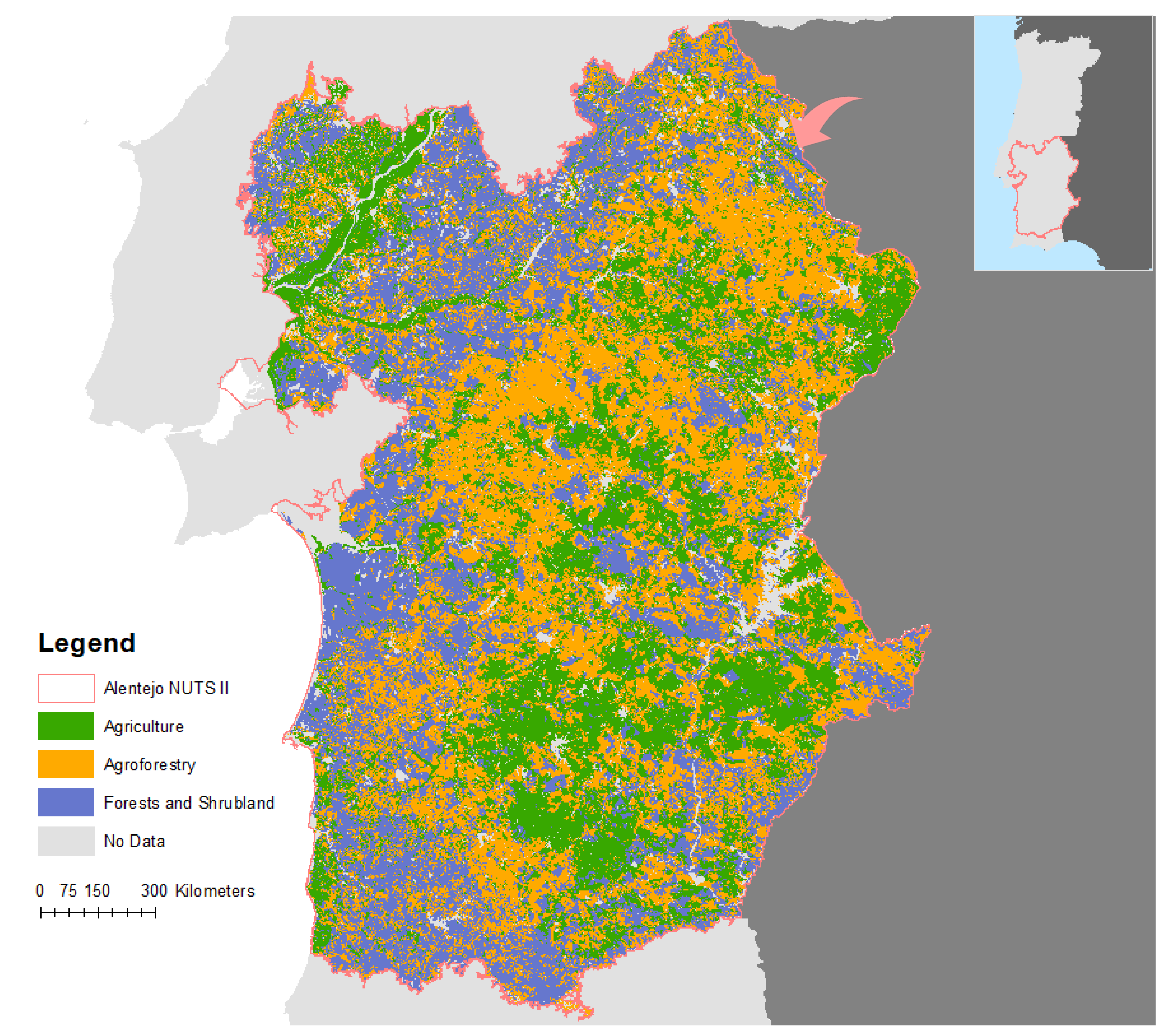
2.1. Study Area
2.2. Mapping Ecosystems’ Condition and Service Supply
2.3. Ecosystem Condition (EC)
2.3.1. Soil Organic Matter
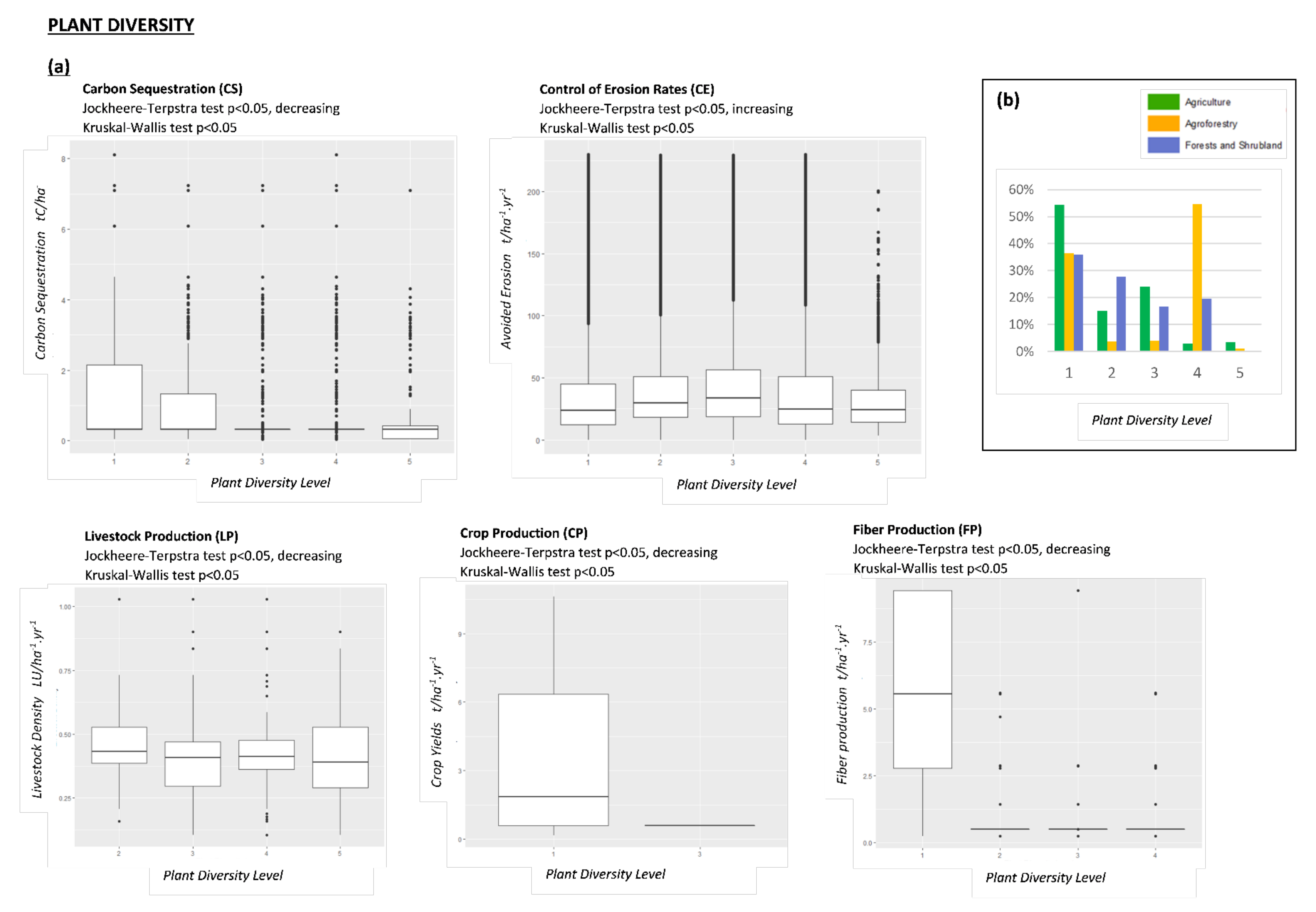
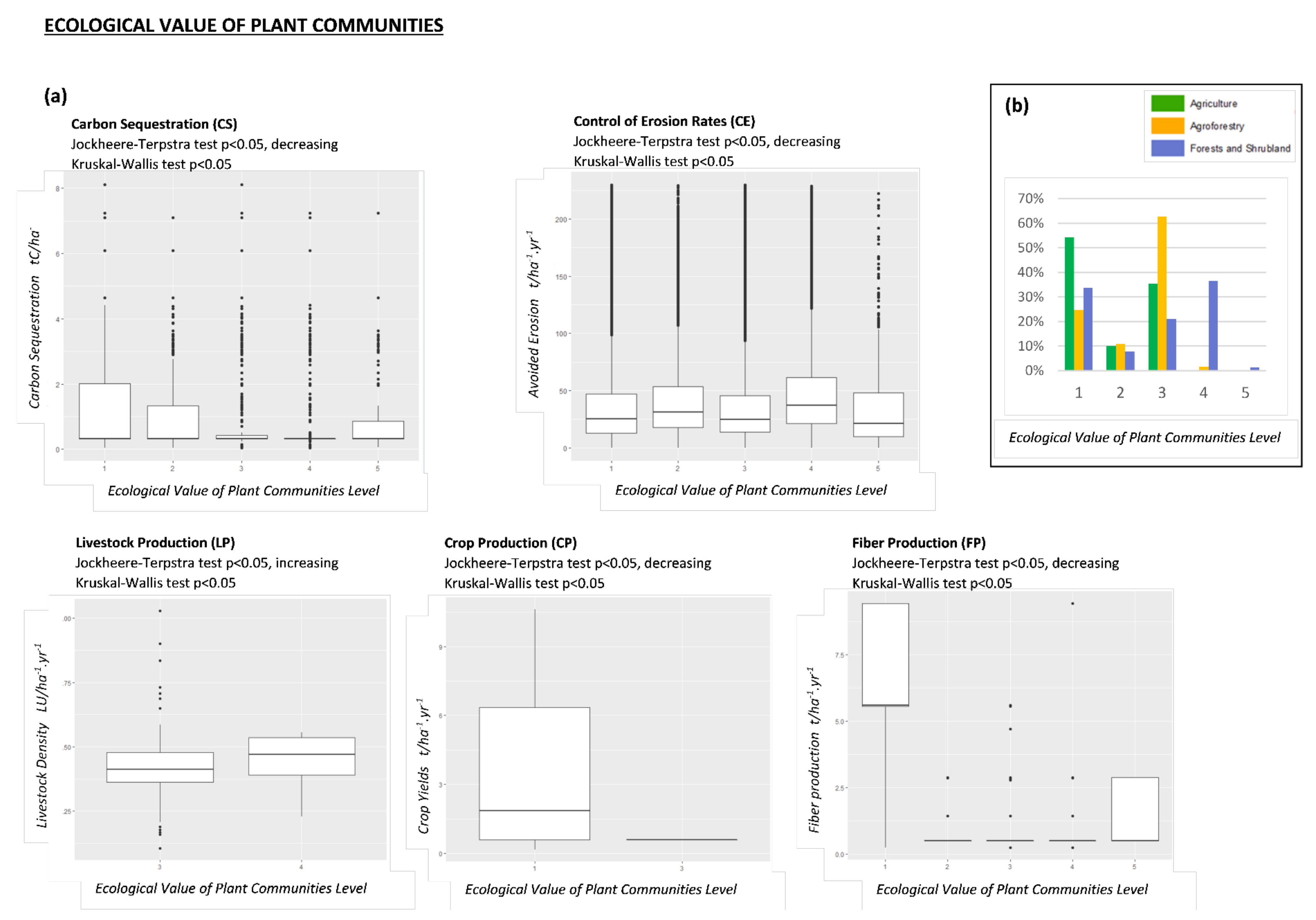
2.3.2. Ecological Value of Plant Communities & Plant Diversity
2.3.3. Bird Diversity
2.4. Ecosystem Services (ES)
2.4.1. Control of Erosion Rates
2.4.2. Climate Regulation through Carbon Sequestration
- Mortality by timber harvesting (spatialization of statistical data allowed determining harvesting rate for the given years at each polygon of interest, i.e., polygons with timber harvesting plantations).
- Mortality by fire (total loss of biomass in polygons that experienced fire events, based on official fire maps for 2007, available at http://www2.icnf.pt/portal/florestas/dfci/inc/mapa (accessed on 1 September 2021)).
- Mortality by transition (total or partial loss of biomass due to land-use transition, from 1990 to 2007, observed in a given polygon).
- Natural mortality, as determined and reported by the NIR (Table 10).

| Forest KP Classes | Mean Annual Increment (m3/ha) |
|---|---|
| 01. Pinus Pinaster | 5.6 |
| 02. Quercus Suber | 0.5 |
| 03. Eucalyptus | 9.5 |
| 04. Quercus Rotundifolia | 0.5 |
| 05. Other Quercus | 2.9 |
| 06. Other Broadleaves | 2.9 |
| 07. Pinus Pinea | 5.6 |
| 08. Other Coniferous | 5 |
| Non-Forest KP Classes | Aboveground Mean Annual Increment | Belowground Mean Annual Increment |
|---|---|---|
| 12. Vineyards | 0.17 | 0.14 |
| 13. Olive | 0.39 | 0.06 |
| 14. Other Permanent | 0.42 | 0.07 |
| 15. Grassland | 0.53 | 0.94 |
| 18. Shrubland | 0.44 | 0.25 |
| Forest KP Classes | Mortality (% of Annual Increment) |
|---|---|
| 01. Pinus Pinaster | 0.77% |
| 02. Quercus Suber | 0.97% |
| 03. Eucalyptus | 0.83% |
| 04. Quercus Rotundifolia | 0.8% |
| 05. Other Quercus | 0.93% |
| 06. Other Broadleaves | 1.23% |
| 07. Pinus Pinea | 0.23% |
| 08. Other Coniferous | 1.1% |
2.4.3. Provisioning ES
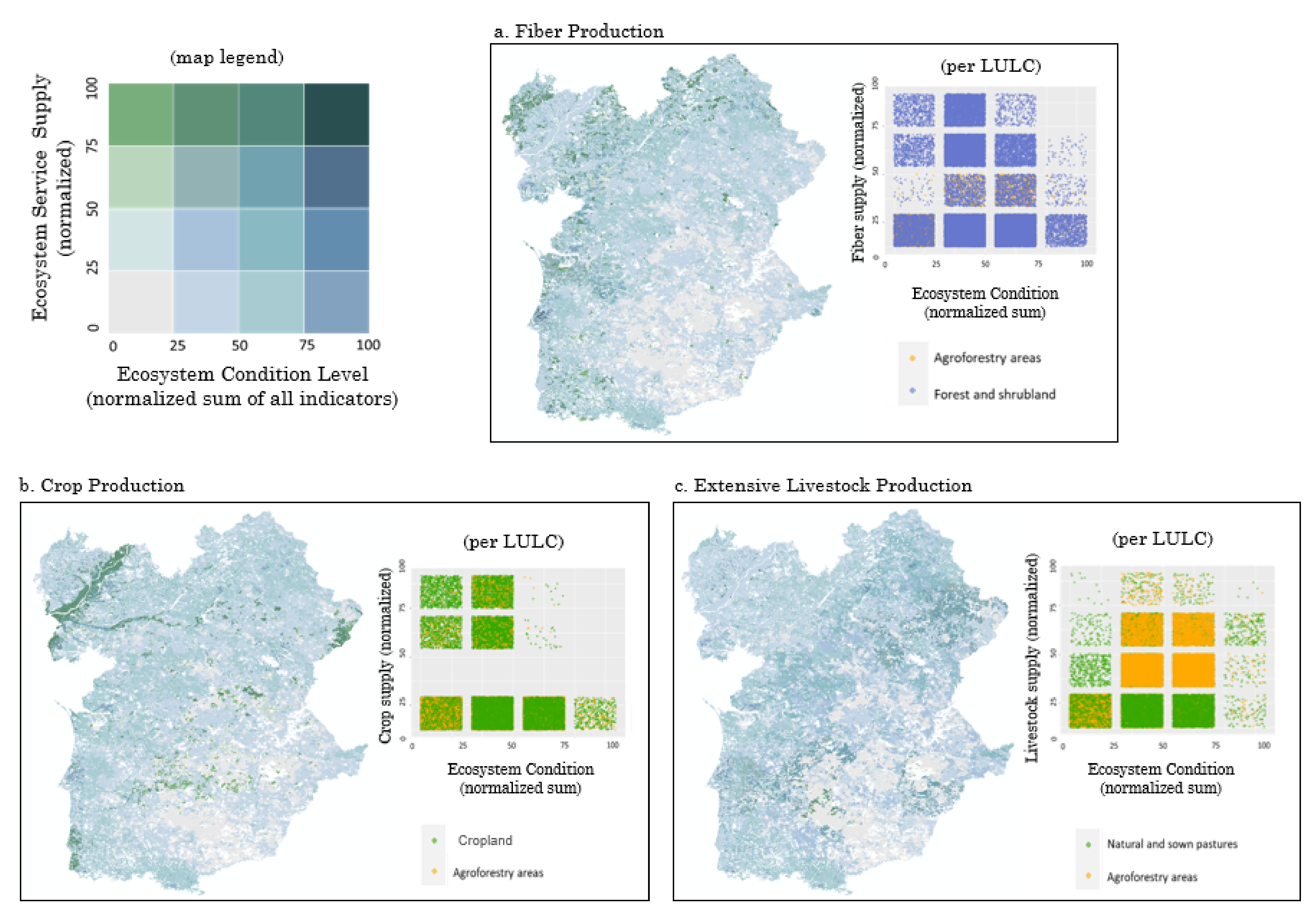
2.5. Spatial Relationships and Interactions
3. Results
3.1. Ecosystem Condition (EC)
3.2. Ecosystem Services (ES)
3.3. Spatial Relationships and Interactions
4. Discussion
4.1. Proposed Analytical Framework
4.2. Spatial Relationships and Interactions
5. Conclusions
Supplementary Materials
Author Contributions
Funding
Institutional Review Board Statement
Informed Consent Statement
Data Availability Statement
Acknowledgments
Conflicts of Interest
| 1 | The 2020 EU Biodiversity Strategy (COM 2011) was built around six mutually supportive and inter-dependent targets that addressed the main drivers of biodiversity loss. They aimed to reduce key pressures on nature and ecosystem services in the EU by setting up efforts to fully implement existing EU nature legislation, anchoring biodiversity objectives into key sectoral policies, and closing important policy gaps. Each target was accompanied by a set of focused, time-bound actions to ensure these ambitions are fully realized. |
| 2 | The goal of Target 2 of the EU Biodiversity Strategy 2020 is to “maintain and restore ecosystems and their services”, with Action 5 set out to “improve knowledge of ecosystems and their services in the EU”. |
| 3 | NUTS II refers to the second level of the Nomenclature of Territorial Units for Statistics (NUTS) that is used in Portugal. |
References
- Millenium Ecosystem Assesment. Ecosystems and Human Well-Being: Synthesis. Millennium Ecosystem Assessment; Island Press: Washington, DC, USA, 2005. [Google Scholar]
- Haines-Young, R.; Potschin, M. Common International Classification of Ecosystem Services (CICES), Version 4.3; Report to the European Environment Agency EEA/BSS/07/007; European Environment Agency: Copenhagen, Denmark, 2013; p. 34.
- Schröter, M.; Barton, D.N.; Remme, R.P.; Hein, L. Accounting for Capacity and Flow of Ecosystem Services: A Conceptual Model and a Case Study for Telemark, Norway. Ecol. Indic. 2014, 36, 539–551. [Google Scholar] [CrossRef]
- Mace, G.M. Whose Conservation? Science 2014, 345, 1558–1560. [Google Scholar] [CrossRef]
- Alexander, S.; Aronson, J.; Whaley, O.; Lamb, D. The Relationship between Ecological Restoration and the Ecosystem Services Concept. Ecol. Soc. 2016, 21, 34. [Google Scholar] [CrossRef] [Green Version]
- Potschin-Young, M.; Haines-Young, R.; Görg, C.; Heink, U.; Jax, K.; Schleyer, C. Understanding the Role of Conceptual Frameworks: Reading the Ecosystem Service Cascade. Ecosyst. Serv. 2018, 29, 428–440. [Google Scholar] [CrossRef]
- Dale, V.H. Ecological Modeling for Resource Management; Springer Science & Business Media: Berlin/Heidelberg, Germany, 2006; ISBN 978-0-387-21563-1. [Google Scholar]
- Maes, J.; Teller, A.; Erhard, M.; Murphy, P.; Paracchini, M.L.; Barredo, J.I.; Grizzetti, B.; Cardoso, A.; Somma, F.; Petersen, J.E.; et al. Mapping and Assessment of Ecosystems and Their Services: Indicators for Ecosystem Assessments under Action 5 of the EU Biodiversity Strategy to 2020; Technical Report (2014-080); Publications Office of the European Union: Luxembourg, 2014; ISBN 978-92-79-36161-6. [Google Scholar]
- Burkhard, B.; Kroll, F.; Nedkov, S.; Müller, F. Mapping Ecosystem Service Supply, Demand and Budgets. Ecol. Indic. 2012, 21, 17–29. [Google Scholar] [CrossRef]
- European Commission. The EU Biodiversity Strategy to 2020; Official Publication of the European Union: Luxembourg, 2011; ISBN 978-92-79-20762-4. [Google Scholar]
- Gonzalez-Redin, J.; Luque, S.; Poggio, L.; Smith, R.; Gimona, A. Spatial Bayesian Belief Networks as a Planning Decision Tool for Mapping Ecosystem Services Trade-Offs on Forested Landscapes. Environ. Res. 2016, 144, 15–26. [Google Scholar] [CrossRef] [PubMed]
- Bruins, R.J.; Canfield, T.J.; Duke, C.; Kapustka, L.; Nahlik, A.M.; Schäfer, R.B. Using Ecological Production Functions to Link Ecological Processes to Ecosystem Services. Integr. Environ. Assess. Manag. 2017, 13, 52–61. [Google Scholar] [CrossRef] [Green Version]
- Cimon-Morin, J.; Darveau, M.; Poulin, M. Fostering Synergies between Ecosystem Services and Biodiversity in Conservation Planning: A Review. Biol. Conserv. 2013, 166, 144–154. [Google Scholar] [CrossRef]
- Maes, J.; Paracchini, M.L.; Zulian, G.; Dunbar, M.B.; Alkemade, R. Synergies and Trade-Offs between Ecosystem Service Supply, Biodiversity, and Habitat Conservation Status in Europe. Biol. Conserv. 2012, 155, 1–12. [Google Scholar] [CrossRef]
- Turkelboom, F.; Leone, M.; Jacobs, S.; Kelemen, E.; García-Llorente, M.; Baró, F.; Termansen, M.; Barton, D.N.; Berry, P.; Stange, E.; et al. When We Cannot Have It All: Ecosystem Services Trade-Offs in the Context of Spatial Planning. Ecosyst. Serv. 2018, 29, 566–578. [Google Scholar] [CrossRef]
- Maes, J.; Teller, A.; Erhard, M.; Liquete, C.; Braat, L.; Berry, P.M.; Egoh, B.; Puydarrieux, P.; Fiorina, F.; Santos, F.; et al. Mapping and Assessment of Ecosystems and Their Services. An Analytical Framework for Ecosystem Assessments under Action 5 of the EU Biodiversity Strategy to 2020; Technical Report (2013-067); Publications Office of the European Union: Luxembourg, 2013; ISBN 978-92-79-29369-6. [Google Scholar]
- Barredo, J.I.; Teller, A.; Bastrup-Birk, A.; Onaindia, M.; de Manuel, B.F.; Madariaga, I.; Rodríguez-Loinaz, G.; Pinho, P.; Nunes, A.; Ramos, A.; et al. Mapping and Assessment of Forest Ecosystems and Their Services: Applications and Guidance for Decision Making in the Framework of MAES; Publications Office of the European Union: Luxembourg, 2016. [Google Scholar]
- Crossman, N.D.; Burkhard, B.; Nedkov, S.; Willemen, L.; Petz, K.; Palomo, I.; Drakou, E.G.; Martín-Lopez, B.; McPhearson, T.; Boyanova, K.; et al. A Blueprint for Mapping and Modelling Ecosystem Services. Ecosyst. Serv. 2013, 4, 4–14. [Google Scholar] [CrossRef]
- Costa, A.; Madeira, M.; Santos, J.L.; Oliveira, Â. Change and Dynamics in Mediterranean Evergreen Oak Woodlands Landscapes of Southwestern Iberian Peninsula. Landsc. Urban Plan. 2011, 102, 164–176. [Google Scholar] [CrossRef]
- Serdoura, F.; Moreira, G.; Almeida, H. Tourism Development in Alentejo Region: A Vehicle for Cultural and Territorial Cohesion. In Proceedings of the Sustainable Architecture and Urban Development, Tripoli, Libya, 3–5 November 2009; Volume 2, pp. 619–634. [Google Scholar]
- Mesquita, S.; Capelo, J.; Gama, I.; Marta-Pedroso, C.; Reis, M.; Domingos, T. Using geobotanical tools to map and assess ecosystem services (MAES) in southern Portugal. In Tools for Landscape-Scale Geobotany and Conservation; Geobotany Studies; Pedrotti, F., Box, E.O., Eds.; Springer International Publishing: Cham, Switzerland, 2021; ISBN 978-3-030-74949-1. [Google Scholar]
- Chambers, S.A.; Australia, B.V. Birds as Environmental Indicators Review of Literature. 2008. Available online: https://www.semanticscholar.org/paper/Birds-as-Environmental-Indicators-Review-of-Chambers-Australia/4d43ad5d64e8c6b097d3e71aa81071c771cec3f8#paper-header (accessed on 1 September 2021).
- Hosmer, D.W., Jr.; Lemeshow, S.; Sturdivant, R.X. Applied Logistic Regression; John Wiley & Sons: Hoboken, NJ, USA, 2013; Volume 398. [Google Scholar]
- Guerra, C.A.; Pinto-Correia, T.; Metzger, M.J. Mapping Soil Erosion Prevention Using an Ecosystem Service Modeling Framework for Integrated Land Management and Policy. Ecosystems 2014, 17, 878–889. [Google Scholar] [CrossRef] [Green Version]
- Wischmeier, W.H.; Smith, D.D. Predicting Rainfall Erosion Losses: A Guide to Conservation Planning; US Department of Agriculture, Science and Education Administration: Washington, DC, USA, 1978; No. 537. [Google Scholar]
- Bakker, M.M.; Govers, G.; van Doorn, A.; Quetier, F.; Chouvardas, D.; Rounsevell, M. The Response of Soil Erosion and Sediment Export to Land-Use Change in Four Areas of Europe: The Importance of Landscape Pattern. Geomorphology 2008, 98, 213–226. [Google Scholar] [CrossRef]
- Pimenta, M.T. Directizes Para Aplicação da Equação Universal da Perda de Solo em SIG. 1999. Available online: https://snirh.apambiente.pt/snirh/download/relatorios/factorC_K.pdf (accessed on 1 September 2021).
- Silva, J.R.C. Fatores da Equaçao Universal de Perdas de Solo e sua conversão para o sistema métrico internacional. Ciên. Agron. Fortaleza 1985, 16, 77–82. [Google Scholar]
- IPCC. Guidelines for National Greenhouse Gas Inventories; Prepared by the National Greenhouse Gas Inventories Programme; Eggleston, H.S., Buendia, L., Miwa, K., Ngara, T., Tanabe, K., Eds.; Intergovernmental Panel on Climate Change (IPCC): Hayama, Japan, 2006; ISBN 978-4-88788-032-0. [Google Scholar]
- APA. Portuguese National Inventory Report on Greenhouse Gases, 1990–2012; Submitted Under the United Nations Framework Convention on Climate Change and The Kyoto Protocol; Portuguese Environment Agency (APA): Amadora, Portugal, 2014. [Google Scholar]
- Jenks, G. The Data Model Concept in Statistical Mapping. Int. Yearb. Cartogr. 1967, 7, 186–190. [Google Scholar]
- Rosário, L. Referências Para a Avaliação Do Sequestro de Carbono Orgânico Nos Solos Portugueses, Com Base Na Rede ICP Forest, Biosoil e LQARS; Relatório AFN/SNIERPA inédito; AFN/SNIERPA: Lisboa, Portugal, 2010. [Google Scholar]
- Kruskal, W.H.; Wallis, W.A. Use of Ranks in One-Criterion Variance Analysis. J. Am. Stat. Assoc. 1952, 47, 583–621. [Google Scholar] [CrossRef]
- Terpstra, T.J. The Asymptotic Normality and Consistency of Kendall’s Test against Trend, When Ties Are Present in One Ranking. Indag. Math. Proc. 1952, 55, 327–333. [Google Scholar] [CrossRef] [Green Version]
- Jonckheere, A.R. A Distribution-Free k-Sample Test Against Ordered Alternatives. Biometrika 1954, 41, 133–145. [Google Scholar] [CrossRef]
- Felipe-Lucia, M.R.; Martín-López, B.; Lavorel, S.; Berraquero-Díaz, L.; Escalera-Reyes, J.; Comín, F.A. Ecosystem Services Flows: Why Stakeholders’ Power Relationships Matter. PLoS ONE 2015, 10, e0132232. [Google Scholar] [CrossRef] [Green Version]
- Reyers, B.; O’Farrell, P.J.; Cowling, R.M.; Egoh, B.N.; Le Maitre, D.C.; Vlok, J.H.J. Ecosystem Services, Land-Cover Change, and Stakeholders: Finding a Sustainable Foothold for a Semiarid Biodiversity Hotspot. Ecol. Soc. 2009, 14, 38. [Google Scholar] [CrossRef] [Green Version]
- Mouchet, M.A.; Rega, C.; Lasseur, R.; Georges, D.; Paracchini, M.-L.; Renaud, J.; Stürck, J.; Schulp, C.J.E.; Verburg, P.H.; Verkerk, P.J.; et al. Ecosystem Service Supply by European Landscapes under Alternative Land-Use and Environmental Policies. Int. J. Biodivers. Sci. Ecosyst. Serv. Manag. 2017, 13, 342–354. [Google Scholar] [CrossRef]
- Rodríguez-Echeverry, J.; Echeverría, C.; Oyarzún, C.; Morales, L. Impact of Land-Use Change on Biodiversity and Ecosystem Services in the Chilean Temperate Forests. Landsc. Ecol. 2018, 33, 439–453. [Google Scholar] [CrossRef]
- Jones, N.; de Graaff, J.; Rodrigo, I.; Duarte, F. Historical Review of Land Use Changes in Portugal (before and after EU Integration in 1986) and Their Implications for Land Degradation and Conservation, with a Focus on Centro and Alentejo Regions. Appl. Geogr. 2011, 31, 1036–1048. [Google Scholar] [CrossRef]
- Morais, T.G.; Silva, C.; Jebari, A.; Álvaro-Fuentes, J.; Domingos, T.; Teixeira, R.F.M. A Proposal for Using Process-Based Soil Models for Land Use Life Cycle Impact Assessment: Application to Alentejo, Portugal. J. Clean. Prod. 2018, 192, 864–876. [Google Scholar] [CrossRef]
- Fezzi, C.; Bateman, I.; Askew, T.; Munday, P.; Pascual, U.; Sen, A.; Harwood, A. Valuing Provisioning Ecosystem Services in Agriculture: The Impact of Climate Change on Food Production in the United Kingdom. Environ. Resour. Econ. 2013, 57, 197–214. [Google Scholar] [CrossRef]
- Kandziora, M.; Burkhard, B.; Müller, F. Mapping Provisioning Ecosystem Services at the Local Scale Using Data of Varying Spatial and Temporal Resolution. Ecosyst. Serv. 2013, 4, 47–59. [Google Scholar] [CrossRef]
- Palma, J.H.N.; Paulo, J.A.; Tomé, M. Carbon Sequestration of Modern Quercus suber L. Silvoarable Agroforestry Systems in Portugal: A YieldSAFE-Based Estimation. Agrofor. Syst. 2014, 88, 791–801. [Google Scholar] [CrossRef]
- Campagne, C.S.; Roche, P.; Müller, F.; Burkhard, B. Ten Years of Ecosystem Services Matrix: Review of a (r)Evolution. One Ecosyst. 2020, 5, e51103. [Google Scholar] [CrossRef]
- Ribeiro, P.F.; Santos, J.L.; Bugalho, M.N.; Santana, J.; Reino, L.; Beja, P.; Moreira, F. Modelling Farming System Dynamics in High Nature Value Farmland under Policy Change. Agric. Ecosyst. Environ. 2014, 183, 138–144. [Google Scholar] [CrossRef]
- Jacobs, S.; Burkhard, B.; Van Daele, T.; Staes, J.; Schneiders, A. ‘The Matrix Reloaded’: A Review of Expert Knowledge Use for Mapping Ecosystem Services. Ecol. Model. 2015, 295, 21–30. [Google Scholar] [CrossRef]
- Perennes, M.; Campagne, C.S.; Müller, F.; Roche, P.; Burkhard, B. Refining the Tiered Approach for Mapping and Assessing Ecosystem Services at the Local Scale: A Case Study in a Rural Landscape in Northern Germany. Land 2020, 9, 348. [Google Scholar] [CrossRef]
- European Environment Agency. Mapping and Assessing the Condition of Europe’s Ecosystems Progress and Challenges: EEA Contribution to the Implementation of the EU Biodiversity Strategy to 2020; Publications Office of the European Union: Luxembourg, 2016.
- Swift, M.J.; Izac, A.-M.N.; van Noordwijk, M. Biodiversity and Ecosystem Services in Agricultural Landscapes—Are We Asking the Right Questions? Agric. Ecosyst. Environ. 2004, 104, 113–134. [Google Scholar] [CrossRef]
- Czúcz, B.; Haines-Young, R.; Kiss, M.; Bereczki, K.; Kertész, M.; Vári, Á.; Potschin-Young, M.; Arany, I. Ecosystem Service Indicators along the Cascade: How Do Assessment and Mapping Studies Position Their Indicators? Ecol. Indic. 2020, 118, 106729. [Google Scholar] [CrossRef]
- Rendon, P.; Steinhoff-Knopp, B.; Saggau, P.; Burkhard, B. Assessment of the Relationships between Agroecosystem Condition and the Ecosystem Service Soil Erosion Regulation in Northern Germany. PLoS ONE 2020, 15, e0234288. [Google Scholar] [CrossRef]
- Daniel, T.C.; Muhar, A.; Arnberger, A.; Aznar, O.; Boyd, J.W.; Chan, K.M.A.; Costanza, R.; Elmqvist, T.; Flint, C.G.; Gobster, P.H.; et al. Contributions of Cultural Services to the Ecosystem Services Agenda. Proc. Natl. Acad. Sci. USA 2012, 109, 8812–8819. [Google Scholar] [CrossRef] [Green Version]
- Vrbičanová, G.; Kaisová, D.; Močko, M.; Petrovic, F.; Mederly, P. Mapping Cultural Ecosystem Services Enables Better Informed Nature Protection and Landscape Management. Sustainability 2020, 12, 2138. [Google Scholar] [CrossRef] [Green Version]
- Burkhard, B.; Santos-Martin, F.; Nedkov, S.; Maes, J. Burkhard B, Santos-Martin F, Nedkov S, Maes J (2018) An operational framework for integrated Mapping and Assessment of Ecosystems and their Services (MAES). One Ecosystem 2018, 3, e22831. [Google Scholar] [CrossRef] [Green Version]
- Smith, A.C.; Harrison, P.A.; Pérez Soba, M.; Archaux, F.; Blicharska, M.; Egoh, B.N.; Erős, T.; Domenech, N.F.; György, Á.I.; Haines-Young, R.; et al. How Natural Capital Delivers Ecosystem Services: A Typology Derived from a Systematic Review. Ecosyst. Serv. 2017, 26, 111–126. [Google Scholar] [CrossRef] [Green Version]
- Silveira, A.; Ferrão, J.; Muñoz-Rojas, J.; Pinto-Correia, T.; Guimarães, M.; Schmidt, L. The sustainability of agricultural intensification in the early 21st century:insights from the olive oil production in Alentejo (Southern Portugal). In Changing Societies: Legacies and Challenges. Vol. 3. The Diverse Worlds of Sustainability; Imprensa de Ciências Sociais: Lisboa, Portugal, 2018; pp. 247–275. ISBN 978-972-671-505-4. [Google Scholar]
- Pereira, H.M.; Reyers, B.; Watanabe, M.; Bohensky, E.; Foale, S.; Palm, C.; Espaldon, M.V.; Armenteras, D.; Tapia, M.; Rincon, A.; et al. Condition and Trends of Ecosystem Services and Biodiversity; Capistrano, D., Samper, C., Samper, K.C., Lee, M.J., Raudsepp-Hearne, C., Eds.; Island Press: Washington, DC, USA, 2005; Volume 4, pp. 171–203. ISBN 978-1-55963-186-0. [Google Scholar]
- Maseyk, F.J.F.; Mackay, A.D.; Possingham, H.P.; Dominati, E.J.; Buckley, Y.M. Managing Natural Capital Stocks for the Provision of Ecosystem Services. Conserv. Lett. 2017, 10, 211–220. [Google Scholar] [CrossRef]
- Pinto-Correia, T.; Ribeiro, N.; Sá-Sousa, P. Introducing the Montado, the Cork and Holm Oak Agroforestry System of Southern Portugal. Agrofor. Syst. 2011, 82, 99. [Google Scholar] [CrossRef] [Green Version]
- Bugalho, M.; Caldeira, M.; Pereira, J.; Aronson, J.; Pausas, J.G. Mediterranean Cork Oak Savannas Require Human Use to Sustain Biodiversity and Ecosystem Services. Front. Ecol. Environ. 2011, 9, 278. [Google Scholar] [CrossRef] [Green Version]
- Esgalhado, C.; Guimarães, H.; Debolini, M.; Guiomar, N.; Lardon, S.; Ferraz de Oliveira, I. A Holistic Approach to Land System Dynamics—The Monfurado Case in Alentejo, Portugal. Land Use Policy 2020, 95, 104607. [Google Scholar] [CrossRef]
- Laporta, L.; Domingos, T.; Marta-Pedroso, C. It’s a Keeper: Valuing the Carbon Storage Capacity of Agroforestry Ecosystems in the Context of CAP Eco-Schemes. Land Use Policy 2021, 109, 105712. [Google Scholar] [CrossRef]


| Selected EC Indicators | Unit | Biophysical Mapping |
|---|---|---|
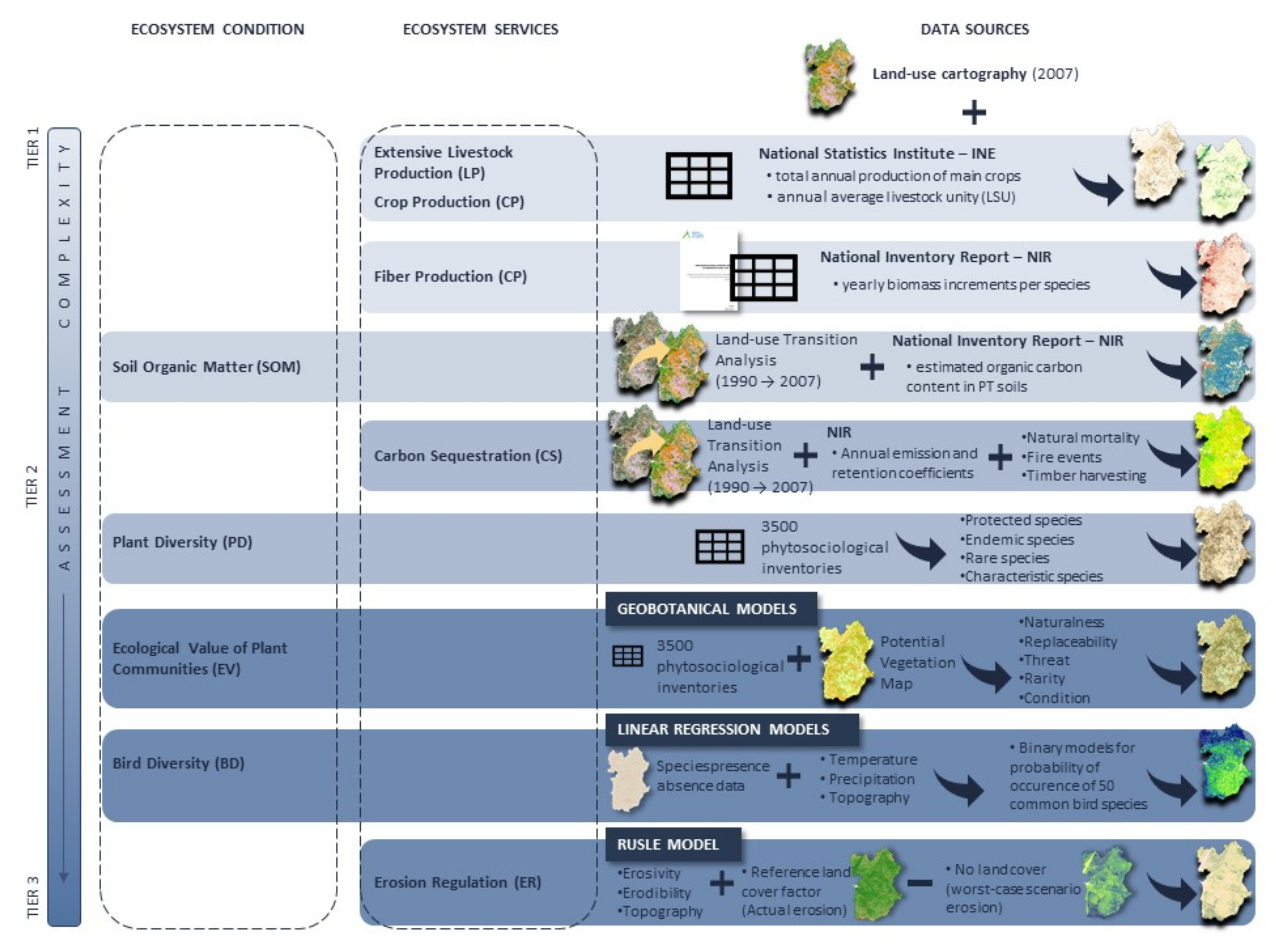
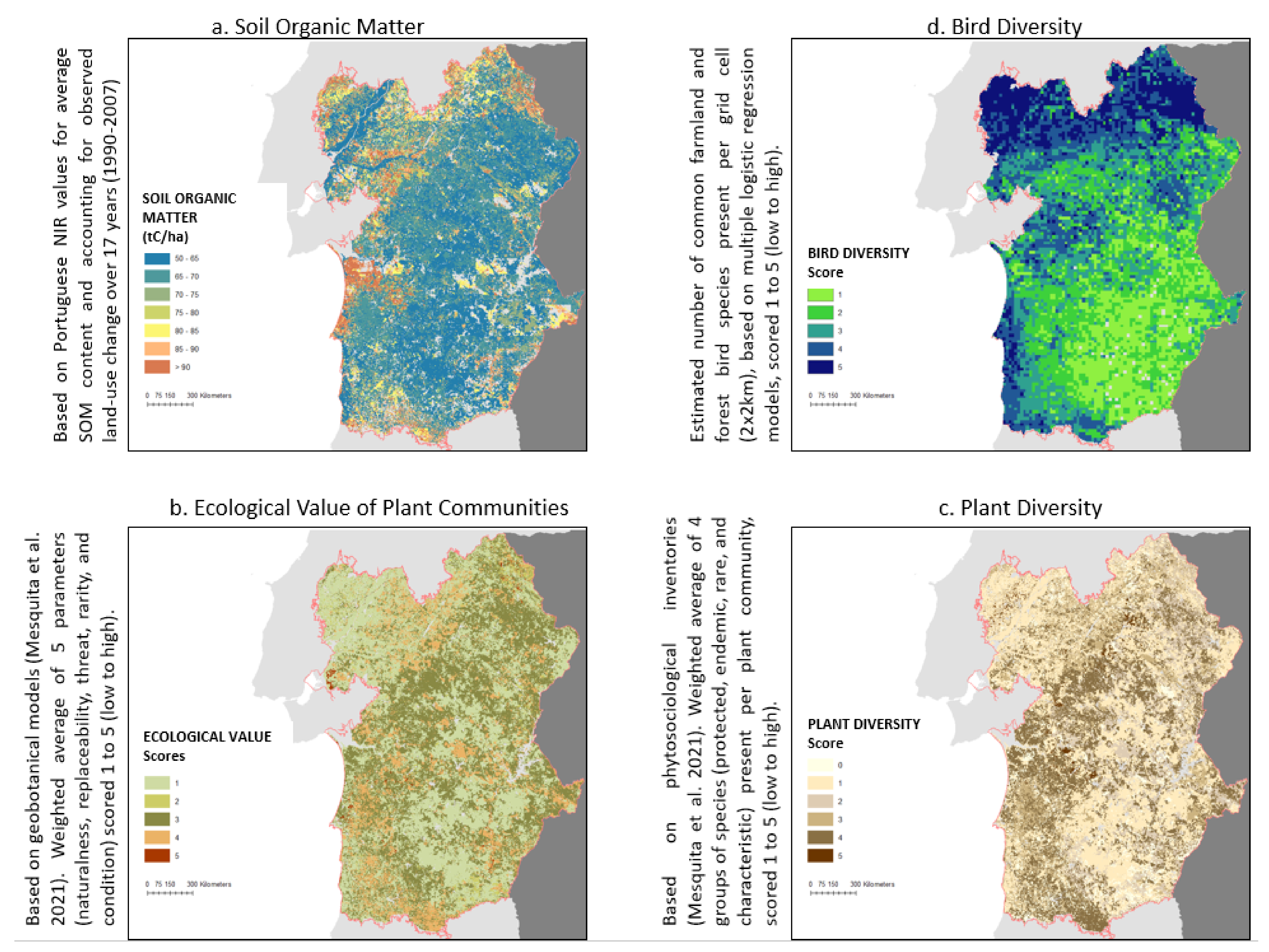
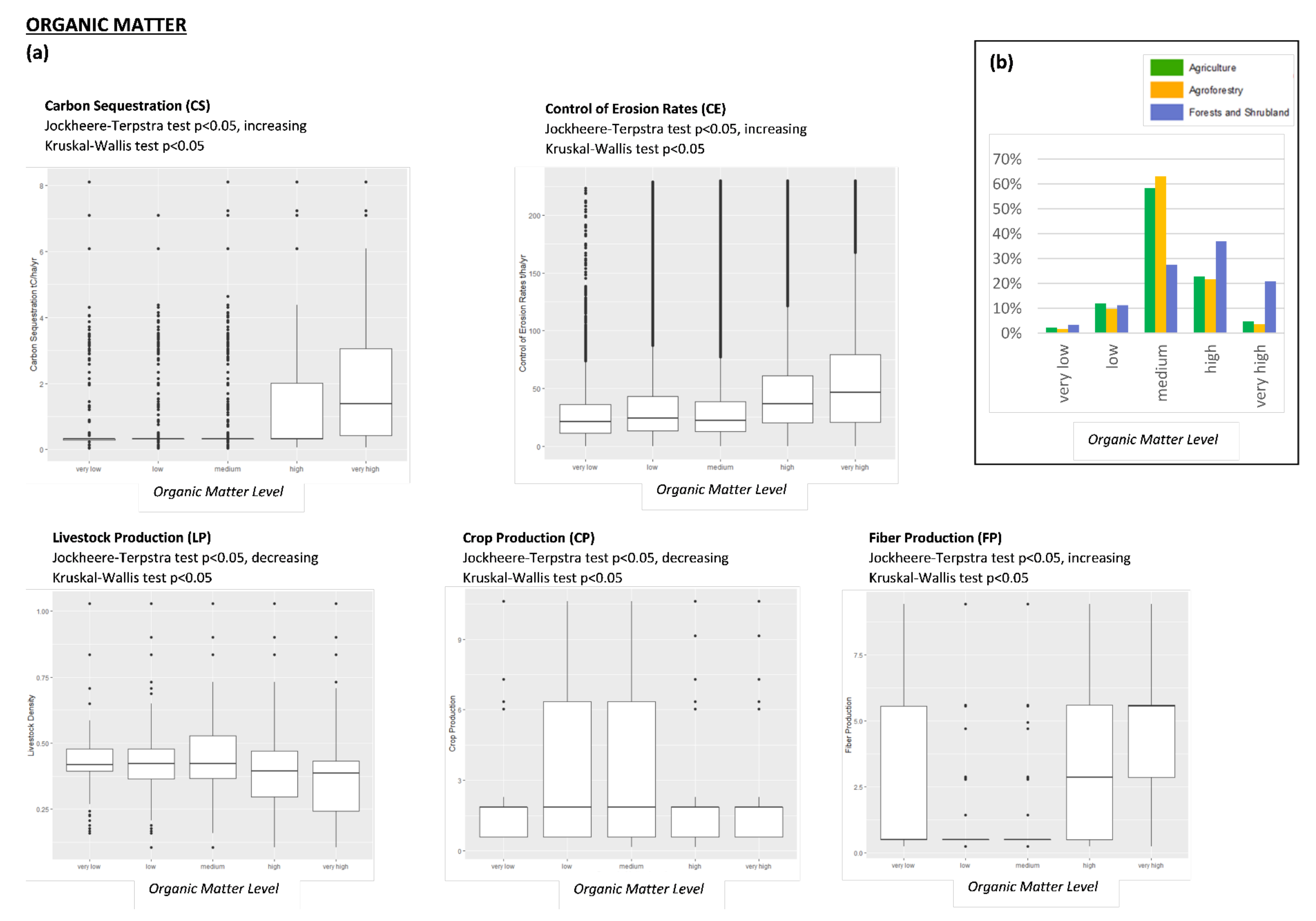
| Soil Organic Matter | tonC.ha−1.year−1 | Soil Organic Matter content was assessed based primarily on the information presented in the National Greenhouse Gases Inventory Report (NIR), according to its land-use typology (Kyoto Protocol classes) although minor adjustments have been introduced (i.e., changes in organic matter estimates in areas undergoing land-use change). Soil organic matter is indicative of the ecological condition of soils, being essential to maintaining soil ecosystem functions such as stabilization, water infiltration, and conservation of nutrients. |
| Ecological Value of Plant Communities | Semi-Quantitative Score (1 to 5) | The Ecological Value of Plant Communities represents the mean value of five parameters (naturalness, replaceability, threat, rarity, and condition), scored from 1 to 5, was attributed to each of the studied ecosystems (level n). The geobotanical models used, at the geographical scale in which they were implemented, are indicative of the ecological condition of ecosystems by providing integrative information on the structural quality, phytocoenotic integrity, and successional maturity of the present plant communities. |
| Plant Diversity | Semi-Quantitative Score (1 to 5) | Plant Diversity Assessment Assumed that Vegetation Series Maps Provide Information on the Natural Communities Occurring at Different Locations. it is thus possible to consult phytosociological tables of these communities and to know their average or characteristic floristic composition, which reflects species richness and rarity, as well as the presence of endemic or threatened species. Based on 3500 phytosociological inventories, representative of Portuguese natural vegetation, plant diversity was estimated as the weighted average of four different parameters attributed to each plant community (presence of protected species, of other endemic species, of other rare species, and of characteristic species). Plant diversity is an indicator of the ecological condition of ecosystems by supporting their multi-functionality and resilience. |
| Bird Diversity | Semi-Quantitative Score (1 to 5) | Indicator Assessment was Based on an Extensive and Publicly Available Dataset of Observation Records (PortugalAves/eBIRD), Used to Obtain a Model (Multiple Logistic Regression with 16 Explanatory Variables Related to Land Use, Temperature, Rainfall and Elevation) that Resulted in a Map with the Potential Distribution of Bird Diversity in the Study Area. This Indicator is thus given by the estimated number of species in grid cells (2 × 2 km) covering the study area, which was reclassified into a 1 (low bird diversity) to 5 (high bird diversity) scale. as can be noted, this differs from the unit of analysis of the other indicators (the LULC polygons from COS07), but this issue has been properly addressed when accounting for spatial relationships. Birds have been widely acknowledged as indicators of the ecological condition of forests and agroecosystems, with bird diversity being one possible good measure of the general ecological condition and overall biodiversity present in an ecosystem. |
| Land-Use Classes | Average tC/ha (0–40 cm) |
|---|---|
| 01. Pinus pinaster | 113 |
| 02. Quercus suber | 66 |
| 03. Eucalyptus spp. | 98 |
| 04. Quercus rotundifolia | 65 |
| 05. Other Quercus spp. | 89 |
| 06. Other broadleaves | 107 |
| 07. Pinus pinea + 08. Other coniferous | 93 |
| 09. Rain-Fed Crops | 59 |
| 10. Irrigated Crops + 11. Rice | 64 |
| 12. Vineyards | 51 |
| 13. Olive | 71 |
| 14. Other Permanent | 56 |
| 15. Grassland | 61 |
| 17. Settlements | 87 |
| 18. Shrubland | 107 |
| UNFCC Category | KP Land-Use Category | Description |
|---|---|---|
| Forest Land | Pinus pinaster | Forests Dominated by Maritime Pine |
| Quercus suber | Forests Dominated by Cork Oak | |
| Eucalyptus spp. | Forests Dominated by Eucalypt Species | |
| Quercus rotundifolia | Forests Dominated by Holm Oak | |
| Quercus spp. | Forests Dominated by Other Oaks | |
| Other broadleaves | Forests Dominated by any Other Broadleaf Species | |
| Pinus pinea | Forests Dominated by Umbrella Pine | |
| Other Coniferous | Forests Dominated by any Other Coniferous Species | |
| Cropland | Rain-Fed Annual Crops | Includes All Land Cultivated with Annual Crops without Irrigation Includes Fallow-Land Integrated Into Crop-Rotations |
| Irrigated Annual Crops | Includes All Land Cultivated with Annual Crops that is Under Irrigation (Except Rice) and Greenhouses | |
| Rice Paddies | Includes All Land Prepared for Rice Cultivation | |
| Vineyards | Includes All Areas Used for Cultivation of Table and/or Wine Grapes | |
| Olive Groves | Includes All Areas Used for Cultivation of Olea Europea146 | |
| Other Permanent Crops | Includes All Areas Used for Cultivation of all other Species of Woody Crops, Including Fruit Orchards147 | |
| Grassland | All Grasslands | Includes All Lands Covered in Permanent Herbaceous Cover |
| Other land | Shrubland | Includes All Lands Covered in Woody Vegetation that do not meet the Forest or Permanent Crop Definitions |
| Variable | Type | Unit | Temporal Scale | Source |
|---|---|---|---|---|
| P/A–Presence/Absence of Each Bird Species | Bird data | Factor (P/A) | 2004–2011 | eBIRD Database |
| tmax–Average Maximum Temperature | Climate and Topography | °C | 2004–2009 | MM5 Model (9 km Resolution) with Krigging (Standard ArcGIS, 1 km Pixel) |
| tmin–Average Minimum Temperature | ||||
| rain–Total Rainfall | mm | |||
| altm–Average Elevation | m | 2009 | DEM (30 m Resolution) Supplied by NASA (ASTER Sensor) * | |
| flor–Forest | Land-use | Factor (P/A) | 2007 | COS’07 Land-Use Cartography (See Supplementary Material Table S1) |
| floa–Open Forest | ||||
| agrs–Rainfed Crops | ||||
| agrr–Irrigated Crops | ||||
| agrp–Permanent Crops | ||||
| agrm–Mixed Crops | ||||
| mont–Montado (Agroforestry Ecosystems) | ||||
| past–Grasslands | ||||
| ncul–Shrublands | ||||
| purb–Urban Settlements | ||||
| plen–Lakes and Other Water Bodies | ||||
| plot–Rivers |
| Scientific Name | Number of Records |
|---|---|
| Saxicola torquatus | 264 |
| Sylvia melanocephala | 259 |
| * Sturnus unicolor | 247 |
| Turdus merula | 246 |
| Parus caeruleus | 240 |
| Parus major | 208 |
| Emberiza calandra | 183 |
| Lanius meridionalis | 182 |
| Fringilla coelebs | 175 |
| Buteo buteo | 169 |
| Carduelis carduelis | 167 |
| Passer domesticus | 163 |
| Erithacus rubecula | 157 |
| * Streptopelia decaocto | 149 |
| * Alectoris rufa | 139 |
| Bubulcus ibis | 138 |
| Galerida cristata | 138 |
| Lullula arborea | 138 |
| Carduelis cannabina | 133 |
| Galerida theklae | 133 |
| Corvus corone | 131 |
| Phylloscopus collybita | 131 |
| Serinus serinus | 128 |
| Oenanthe oenanthe | 125 |
| Cisticola juncidis | 124 |
| Garrulus glandarius | 123 |
| Motacilla alba | 118 |
| * Pica pica | 117 |
| Falco tinnunculus | 116 |
| Upupa epops | 116 |
| Cyanopica cyanus | 115 |
| Carduelis chloris | 112 |
| Columba palumbus | 107 |
| Sylvia atricapilla | 107 |
| Ardea cinerea | 106 |
| Sitta europaea | 104 |
| Certhia brachydactyla | 102 |
| Anthus pratensis | 97 |
| Cettia cetti | 94 |
| Elanus caeruleus | 81 |
| Ficedula hypoleuca | 80 |
| * Troglodytes troglodytes | 80 |
| Hirundo rustica | 78 |
| * Vanellus vanellus | 77 |
| Egretta garzetta | 74 |
| * Anas platyrhynchos | 72 |
| Hirundo daurica | 72 |
| * Turdus philomelos | 67 |
| * Tringa ochropus | 65 |
| * Dendrocopos major | 62 |
| Bird Diversity Scale | # of Species Present (p > 0.5) |
|---|---|
| 1 | [0;5] |
| 2 | [6;9] |
| 3 | [10;13] |
| 4 | [14;17] |
| 5 | [18;…] |
| Selected ES | Biophysical Mapping | ||||
|---|---|---|---|---|---|
| ES Classification Following CICES (v5.1) | Specifications | ||||
| Section | Section | Class (Code) | ES Designation | Indicator Unit | Description |
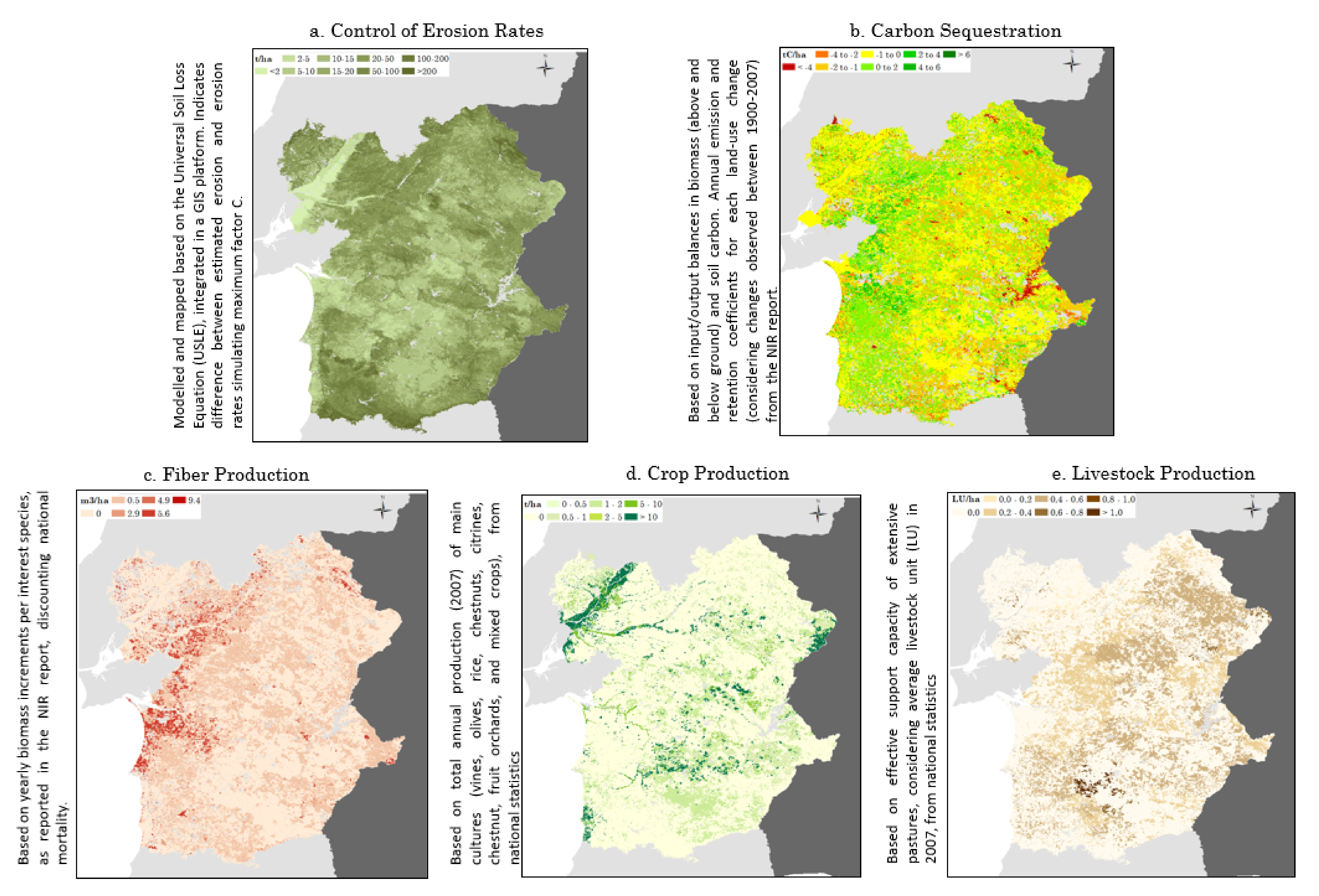
| Provisioning | Biomass | Cultivated Crops (1.1.1.1) | Crop Production | ton.ha−1.yr−1 | Crop Production was mapped based on the total annual production of main cultures present within the study area. Information obtained per municipality, based on official national agriculture statistics (Instituto Nacional de Estatística, INE). Spatialization of this information was possible based on the harmonization of culture classes with LULC classes. |
| Reared Animals and Their Outputs (1.1.1.2) | Extensive Livestock Production | L LU.ha−1.yr−1 | Extensive Livestock Production was mapped based on the effective support capacity of extensive pastures, considering the average livestock unit (LU) within the study area. Information obtained per municipality, based on official national agriculture statistics (Instituto Nacional de Estatística, INE). Spatialization of this information was possible based on the harmonization of pasture classes with LULC classes | ||
| Fibers and Other Materials for Direct Use or Processing (1.2.1.1) | Fiber Production | m3.ha−1.yr−1 | Fiber Production mapping was based on yearly biomass increments per species, as reported in the Portuguese National Greenhouse Gases Inventory Report (NIR), According to its land-use typology (Kyoto Protocol Classes). classes of species considered were: Pinus pinaster, Pinus pinea, Quercus spp, Quercus suber, Quercus rotundifolia, Eucalyptus spp, Mixed broadleaves forests, and mixed coniferous forests. average biomass losses due to natural mortality were discounted. spatialization of this information was possible based on the harmonization of kp classes legend with LULC classes from national cartography. | ||
| Regulating | Regulation of Physical, Chemical, Biological Conditions | Global Climate Regulation by Reduction of Greenhouse Gas Concentrations (2.3.5.1) | Carbon Sequestration | tonCO2.ha−1.yr−1 | Carbon Sequestration mapping was based on input/output balances in biomass (above and below ground). Annual emission and retention coefficients for each land-use change (considering changes observed in a 17-year period) were estimated based on the National Inventory Report results (NIR). Spatialization of this information was possible based on the harmonization of KP classes legend with LULC classes from national cartography. |
| Stabilization and Control of Erosion Rates (2.2.1.1) | Control of Erosion Rates | ton.ha−1.yr-−1 | Control of Erosion Rates was modeled and mapped based on the Universal Soil Loss Equation (USLE), integrated into a GIS platform, which allowed determining the difference between erosion rates in the current scenario (i.e., erosion rates given actual land cover type) and erosion rates for a worst-case scenario (considering a maximum erosion cover type), as first suggested by [24] | ||
Publisher’s Note: MDPI stays neutral with regard to jurisdictional claims in published maps and institutional affiliations. |
© 2021 by the authors. Licensee MDPI, Basel, Switzerland. This article is an open access article distributed under the terms and conditions of the Creative Commons Attribution (CC BY) license (https://creativecommons.org/licenses/by/4.0/).
Share and Cite
Laporta, L.; Domingos, T.; Marta-Pedroso, C. Mapping and Assessment of Ecosystems Services under the Proposed MAES European Common Framework: Methodological Challenges and Opportunities. Land 2021, 10, 1040. https://doi.org/10.3390/land10101040
Laporta L, Domingos T, Marta-Pedroso C. Mapping and Assessment of Ecosystems Services under the Proposed MAES European Common Framework: Methodological Challenges and Opportunities. Land. 2021; 10(10):1040. https://doi.org/10.3390/land10101040
Chicago/Turabian StyleLaporta, Lia, Tiago Domingos, and Cristina Marta-Pedroso. 2021. "Mapping and Assessment of Ecosystems Services under the Proposed MAES European Common Framework: Methodological Challenges and Opportunities" Land 10, no. 10: 1040. https://doi.org/10.3390/land10101040
APA StyleLaporta, L., Domingos, T., & Marta-Pedroso, C. (2021). Mapping and Assessment of Ecosystems Services under the Proposed MAES European Common Framework: Methodological Challenges and Opportunities. Land, 10(10), 1040. https://doi.org/10.3390/land10101040