Article

Climate Variability Structures Plant Community Dynamics in Mediterranean Restored and Reference Tidal Wetlands

by
Dylan E. Chapple
1,*,
Phyllis Faber
2,
Katharine N. Suding
3 and
Adina M. Merenlender
1
1
Department of Environmental Science, Policy and Management, University of California, Berkeley, 137 Mulford Hall, Berkeley, CA 94720, USA
2
765 Miller Ave, Mill Valley, CA 94941, USA
3
Institute of Arctic and Alpine Research, University of Colorado, Boulder, Boulder, CO 80309, USA
*
Author to whom correspondence should be addressed.
Water 2017, 9(3), 209; https://doi.org/10.3390/w9030209
Submission received: 11 November 2016 / Revised: 21 February 2017 / Accepted: 7 March 2017 / Published: 13 March 2017

Abstract

:
In Mediterranean regions and other areas with variable climates, interannual weather variability may impact ecosystem dynamics, and by extension ecological restoration projects. Conditions at reference sites, which are often used to evaluate restoration projects, may also be influenced by weather variability, confounding interpretations of restoration outcomes. To better understand the influence of weather variability on plant community dynamics, we explore change in a vegetation dataset collected between 1990 and 2005 at a historic tidal wetland reference site and a nearby tidal wetland restoration project initiated in 1976 in California’s San Francisco (SF) Bay. To determine the factors influencing reference and restoration trajectories, we examine changes in plant community identity in relation to annual salinity levels in the SF Bay, annual rainfall, and tidal channel structure. Over the entire study period, both sites experienced significant directional change away from the 1990 community. Community change was accelerated following low salinity conditions that resulted from strong El Niño events in 1994–1995 and 1997–1998. Overall rates of change were greater at the restoration site and driven by a combination of dominant and sub-dominant species, whereas change at the reference site was driven by sub-dominant species. Sub-dominant species first appeared at the restoration site in 1996 and incrementally increased during each subsequent year, whereas sub-dominant species cover at the reference site peaked in 1999 and subsequently declined. Our results show that frequent, long-term monitoring is needed to adequately capture plant community dynamics in variable Mediterranean ecosystems and demonstrate the need for expanding restoration monitoring and timing restoration actions to match weather conditions.

1. Introduction

The practice of restoring native plant communities aims to facilitate transitions between degraded and ecologically functional landscapes by manipulating abiotic [1,2,3] and biotic conditions [4]. However, transitions from a degraded state to a desirable state depend not only on actions taken at discrete sites, but also on regional climate and weather [5,6,7]. Research on the impacts of spatial and environmental determinants of restoration outcomes has developed steadily [8,9,10], but detailed temporal studies that capture interannual dynamics in highly variable climates are still under-represented in the literature [7,11]. Restored sites can take many years to match conditions at reference sites [12], which may have impacts on the conservation benefits that restoration projects purport to offer [13,14]. Understanding the role of climate and weather in determining plant community dynamics will be essential for managing restoration projects into the future.
Mediterranean climates and other arid and semi-arid systems around the world are characterized by high interannual weather variability (high coefficient of variation for precipitation) [5,15,16], which may impact plant species dynamics [17,18], and by extension, restoration outcomes [19]. These changes in weather can lead systems down different trajectories depending on where and when projects are initiated [20]. Without long-term data, it is challenging to know whether observed changes at restoration sites are true trends or simply transient effects [21]. For example, initial increases in native plant diversity following restoration may decline over time [22], leading to false interpretations of restoration outcomes if too short an evaluation window is assessed. These spurious conclusions may influence restoration management and policy [7]. While theory in this regard has gained acceptance, the consideration of temporal variability in weather when implementing and evaluating restoration has lagged behind [7,11].
Integrating contingencies related to climate into planning and monitoring efforts has high potential to improve management outcomes. For most restoration projects, a 5-year monitoring plan is the best case scenario, and monitoring may not even be part of the project funding structure [23,24,25]. However, wet and dry years may exist consecutively, with extended periods of drought interspersed with pockets of heavy rainfall. Ecological communities may also respond in subsequent (lag) years or be further influenced by species interactions that are contingent on weather [26]. The uncertainty and variability of weather and its influence on ecological communities may create mismatches between project timing and weather conditions that would favor success [19]. Despite a pressing need to understand these dynamics, a recent meta-analysis identified a lack of studies using long-term data to investigate the influence of interannual variability on restoration outcomes [11].
Our study explores tidal marsh plant community dynamics at a restoration and a reference site in California’s San Francisco (SF) Bay over a 15-year period. Mediterranean ecosystems like the SF Bay are defined by dry summers and intermediately wet winters, with a high coefficient of variation for precipitation from year to year [16,27]. In tidal systems in California, salinity is influenced by drought conditions that can significantly reduce the amount of precipitation delivered and El Niño events that can increase rainfall and snowpack [15]. Work from the Tijuana Estuary in southern California demonstrated that primary productivity of the tidal wetland co-dominant Spartina foliosa increases during periods of higher freshwater flows related to El Niño events and declines in years with higher salinity [28,29]. Other studies show the importance of lowered salinity for seed emergence in high marsh species [30], increased abundance of salt sensitive species following experimental freshwater addition [31,32], and the importance of periods of high rainfall in structuring tidal marsh restoration outcomes [33]. Historic analyses of pollen samples in a tidal wetland in the south SF Bay show that species composition can vary markedly across time, likely in response to freshwater dynamics [34]. El Niño events have been shown to influence densities of microbenthic organisms in California marshes by homogenizing community composition across reference and restored marshes [35]. These types of shifts can impact food web dynamics for faunal communities that subsequently interact with plant distributions [36,37,38], underscoring the fact that changes in plant distributions have the potential to impact a range of other tidal wetland organisms. This highlights the importance of understanding plant community responses to weather variability, which may be a central factor controlling restoration trajectories in Mediterranean ecosystems [19,39]. These areas are expected to be hotspots of climate change over the coming century, increasing uncertainty and variability [40]. While Mediterranean ecosystems are relatively rare globally, increased variability is a projected outcome of the changing climate across the globe [41] and the lessons learned from these regions will only become increasingly relevant in a variety of ecosystems worldwide.
In our study, we focus on California tidal wetlands, where salinity [31,40], channel structure [42,43], species dynamics [44], and elevation [34] interact to influence species composition, and shifts in salinity can alter productivity [28] and species composition [31]. Furthermore, since plant community restoration in the SF Bay is largely driven by passive seed dispersal via tidal waters (hydrochory) [45], dynamics at restoration sites may be related to the dynamics in adjacent reference sites [46]. In the SF Bay, a complex set of upstream interactions in the Sierra Nevada and Central Valley determine salinity levels, which are generally higher in areas closer to the Pacific Ocean and vary throughout the year in response to snowmelt, human diversions, and other factors [15]. Consequently, variation in Bay salinity levels may be a better predictor of plant community transitions than local rainfall, which may only minimally influence salinity in sites inundated by the tide twice daily [40].
To better understand the influence of interannual weather variability on restoration outcomes, we analyzed a long-term data set of plant community composition collected at one reference and one restoration site between 1990 and 2005. These studies were initially set up as part of an effort by the California Coastal Conservancy to better understand restoration trajectories over time in order to plan and manage future projects [47]. To our knowledge, this data set is one of the longest continuous data sets comparing a tidal wetland reference and restoration site. To explore how regional salinity, local rainfall, and site topography influence plant community trajectories, we look at SF Bay salinity adjacent to the sites, rainfall, and channel structure.

2. Materials and Methods
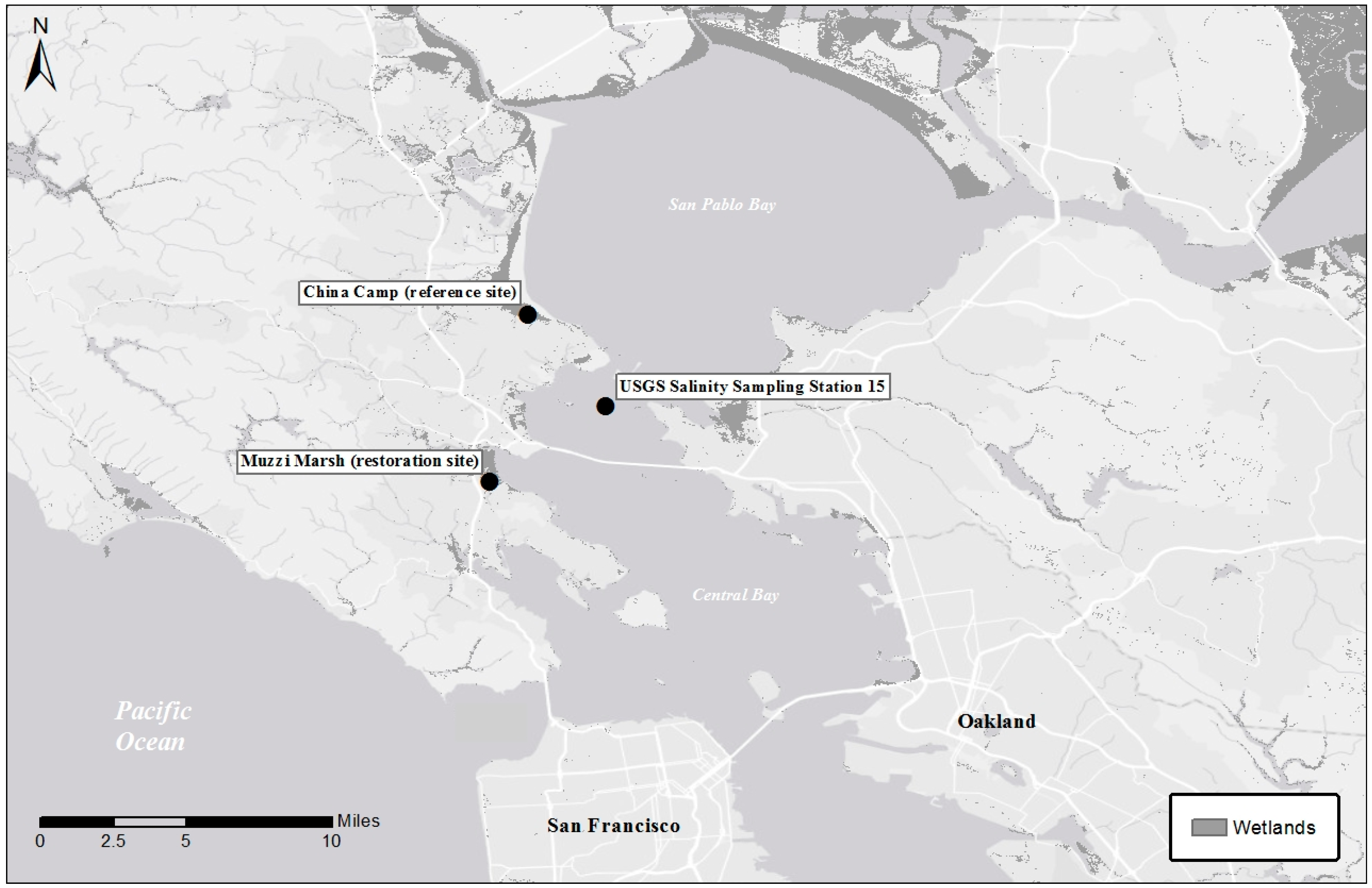
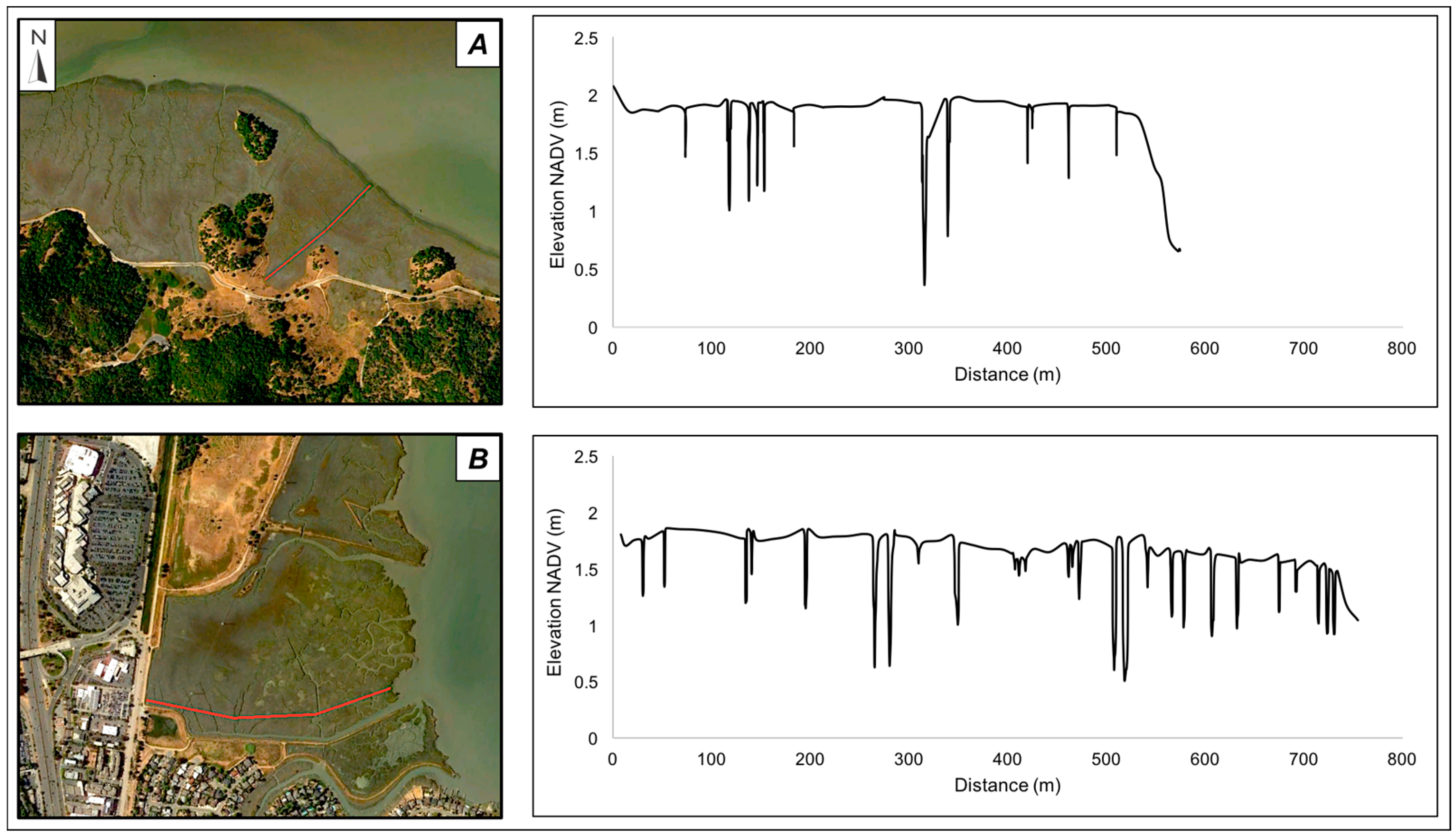
2.1. Sites

The San Francisco Bay (SF Bay; 37°50′37 N, 122°21′46 S) is a tidal estuary in central California, USA whose watershed drains the majority of the western side of the Sierra Nevada through the Central Valley [15]. The area is characterized by a Mediterranean climate, with a wet season extending from October through April and a dry season extending from May through September [15]. Beginning in the mid-1800s, widespread land conversion led to the destruction of approximately 79% of historic wetlands, and since the early 1970s, over 17,000 acres have been restored (Goals Update 2015). We collected data at a tidal wetland reference site (China Camp State Park, San Rafael, CA, USA; 38°00′36 N 122°30′25 S; Figure 1, now part of the SF Bay National Estuarine Research Reserve) and restoration site initiated in 1976 (Muzzi Marsh, Corte Madera, CA, USA; 37°55′36 N 122°30′25 S; Figure 1, now part of the Corte Madera State Ecological Reserve) [47,48]. China Camp State Park is an approximately 5000 year old tidal salt marsh [47]. The site is notable for its intact transitions from wetland to upland, a rarity in the heavily altered SF Bay. Due to the low amount of alteration at the site, it is commonly used as a reference for pre-disturbance tidal wetland conditions in the area [48,49]. Muzzi Marsh is one of the earliest tidal marsh restoration projects in the SF Bay [48], and our data collection began 14 years after the initial restoration actions. Roughly half of the study area was filled with dredge material prior to tidal breaching, and the remainder of the area increased in elevation through passive sedimentation. Tidal channels were slow to form in the filled area, an insight that led to abandoning the idea of filling sites with material prior to breaching levees for restoration [47]. Neither site has significant direct links to upland freshwater outflow, with China Camp at approximately 1400 m and Muzzi Marsh at approximately 1700 m from the nearest major freshwater source.

2.2. Field Data Collection

Study plots were established in 1990 to better understand how reference and restoration site conditions change over time, and preliminary work on the data can be found in Williams and Faber 2004 [47]. At each site, a series of consecutive 15.2 m (50 ft) linear plots were established, extending from the upland transition edge to the end of the marsh plain (Figure 2). Plots were marked with plastic pipes for repeat surveys, nearly all of which were present when we re-visited the sites in 2015. Vegetation composition was collected by stretching a meter tape between the markers at the beginning and end of each plot and determining the percent vegetation cover of each species along the linear section of the meter tape [47]. Elevation was surveyed in 2005 using a total station related to a permanent benchmark at each site and elevation data was converted from the National Geodetic Vertical Datum (NGVD 1927) to the North American Vertical Datum (NADV 1988) (Figure 2). To determine the elevation of the marsh plain at each site, we excluded tidal channels from the data and calculated the mean. The number of tidal channels crossing through each plot was also determined for inclusion in statistical models. Each year, vegetation was sampled in late June or early July to capture peak biomass and species composition. Due to differences in site size, data was collected from 33 plots at the reference site and 45 plots at the restoration site for most years between 1990 and 2005. Due to funding restrictions, species composition data was not taken in 1991, 1993, 1997, 2000, or 2001 at the reference site or in 1991, 1993, or 2000 at the restoration site. Our methodologies for working with the missing years is detailed in the Data Analysis section below. To determine how the sites had progressed since 2005, we collected data at both sites in September of 2015, following 4 years of historic drought in the area.

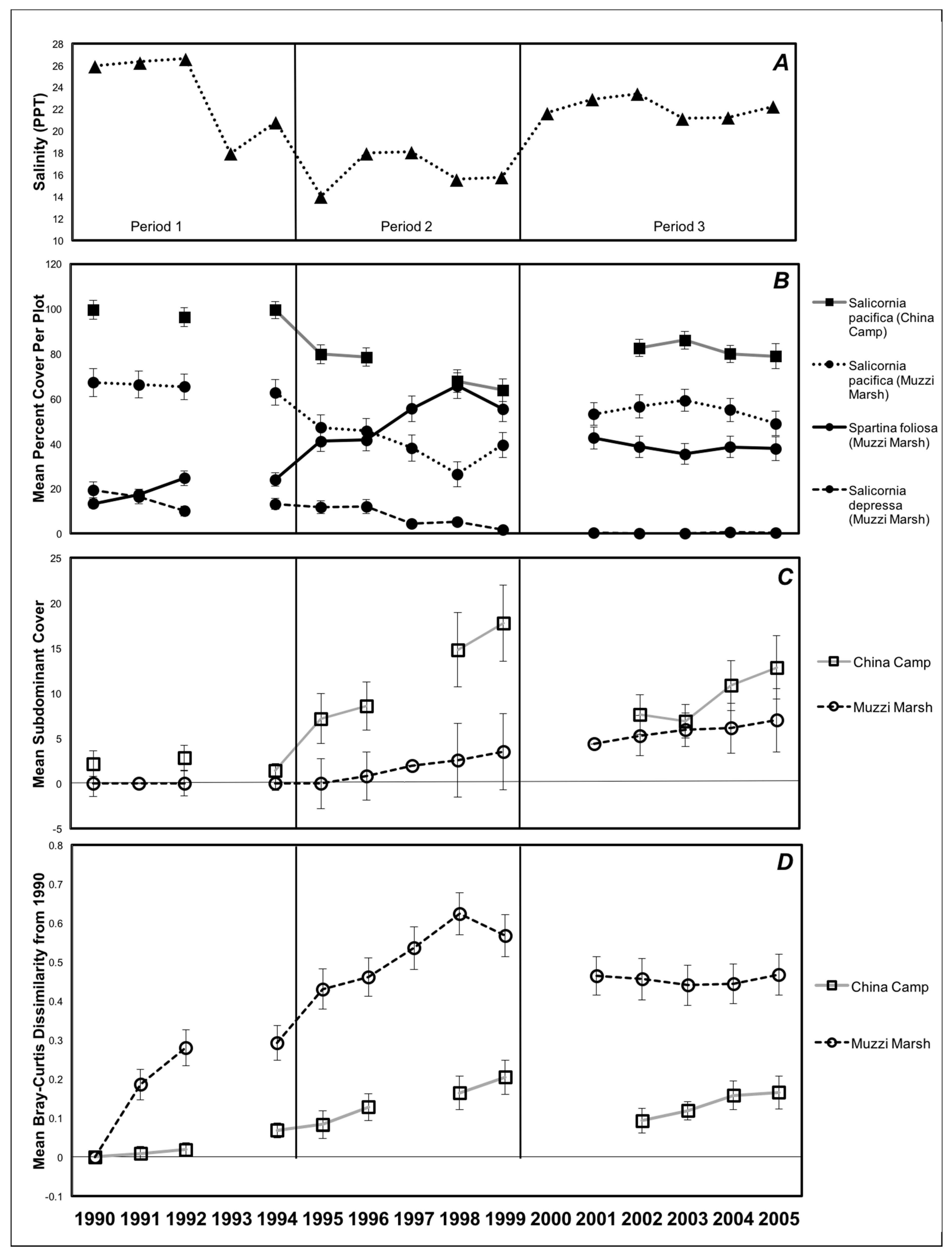
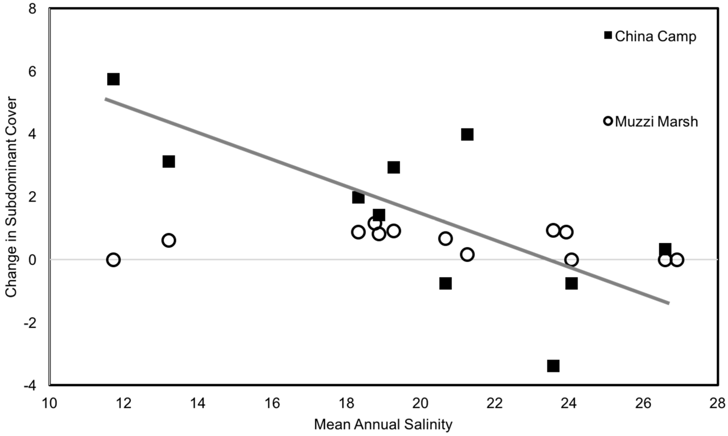
2.3. Salinity and Rainfall

Bay salinity in parts per thousand (PPT) was taken from the US Geologic Survey (USGS) water quality cruises initiated in 1990 [50]. Salinity is a primary determinant of species distributions in the SF Bay, and is likely to be significantly influenced in both timing and magnitude by climate change [40]. Bay salinity is determined by stream and river flow from the Sierra Nevada, and to a certain extent by upstream management of flows [15]. Our salinity data was taken from Station 15 of the USGS San Francisco Bay water quality cruise data set (Figure 1) [51]. Due to the close proximity of this sampling station to the sites and the lack of direct freshwater flow into either site, this data is an adequate proxy for site-level salinity. To determine monthly averages, mean salinity was taken from the two upper sampling depths. For most months, two sampling dates were available to determine the monthly mean. If only one sampling date was available, it was used as the monthly mean. We calculated rainfall for each rain year using National Oceanic and Atmospheric Administration (NOAA) weather station data from Muir Woods National Monument in Mill Valley, Marin County, CA, USA [52]. This data set was the only local data set that encompassed the entire study period without significant gaps, and was roughly equidistant from the two sites, so it was used for both sites. Daily precipitation was collected in mm, summed to produce monthly totals, and was then used to determine rain year means. To determine the annual salinity and rainfall means, we aggregated data by rain year, stretching from October to September of each set of consecutive years. Years are referred to by vegetation sampling date, (e.g., 1995) for time periods encompassing the previous rain year (e.g., October 1994–September 1995). These two data sources provide relatively high-temporal resolution that is necessary for interpreting community change over time. Notably, our study period begins at the end of a major drought (1990–1992) and includes 2 major El Niño years (winters 1994–1995 and 1997–1998) that brought above average precipitation at the local and watershed scale, and subsequently lowered salinity levels in the SF Bay.

2.4. Data Analysis

To assess change in sub-dominant species between years, we calculated the total percent cover of sub-dominant species each year and subtracted the previous year’s total cover. The species included in this analysis are Frankenia salina (Alkali Heath), Distichlis spicata (Saltgrass), Jaumea carnosa (Fleshy Jaumea), and Grindelia stricta (Marsh Gumplant). These species are more sensitive to salinity [33,40] and less abundant in restoration sites compared to the dominant species Salicornia pacifica (Pickleweed) and Spartina foliosa (Pacific Cordgrass) [47], so they provide valuable insight into community dynamics. Because tidal wetland restoration in the SF Bay is largely driven by seed arrival through hydrochory [45], sub-dominant species were not actively planted at either site. To account for missing years, the sub-dominant change was divided by the number of missing years (for example, a change of 2% from 1992 to 1994 with 1993 missing was divided into a 1% change per year). We took the means of salinity and rainfall for the years in question (for example, for assessing change between 1992 and 1994, we took the mean of salinity during the 1993 and 1994 rain years) and used these in our models to avoid over-weighting the adjusted data for missing years. In our resulting models, change over missing periods is included as a single data point per plot. We ran models with and without the additional years included, and it did not change the significance of the outputs, so we elected to present results from the more conservative approach.
To determine community change across time, we used a Bray-Curtis dissimilarity metric to examine plot-level species turnover at each site [18]. These metrics sum the absolute value of species abundance differences between year A and year B and divide this sum by the total abundance of species found in each plot across both years [53]. We removed bare ground from our cover data, calculated the relative abundance of each species in each plot, log transformed the data, and used the Vegan package in R [54] to determine the change relative to the initial (1990) community and for each combination of pairwise years (e.g., 1994–1995). For change from the initial community, we did not estimate values for the missing year averages since we were interested in directional trends, which are discernable without the replacement of missing years. For change between pairwise years, we divided the dissimilarity value for the available pairwise combination (e.g., 1992–1994) by the number of years to generate the mean annual change for that year. We elected not to use overall species diversity as a metric for this analysis, because the reference site did not include significant amounts of Spartina foliosa or Salicornia depressa, which heavily influenced the diversity analysis.
To determine the influence of salinity and rainfall on sub-dominant species, we first used generalized additive models to look at the influence of mean annual salinity and rainfall on the change in sub-dominant species abundance. We elected to use this non-parametric approach because salinity and rainfall data were correlated and collected from the same location across multiple years and thus were not truly independent. For each site, the mean change in sub-dominant abundance for pairwise years was the dependent variable, and log transformed mean salinity and rainfall were the independent variables. Generalized additive models were fit using the GAM package in R [55].
To explore the change over time relative to the initial community across time, we divided the data into three periods based on the influence of the major 1995 and 1998 El Niño events on Bay salinity: period 1 (1990–1994; mean salinity = 22.92 ppt), period 2 (1995–1999; mean salinity = 16.28 ppt), and period 3 (1999–2005; mean salinity = 22.79 ppt). 1990–1992 encompassed the end of a major drought in California (Figure 3). To determine differences in salinity levels between the three periods, we used linear mixed models with year and salinity sample depth as random effects, and time period as the fixed effect.
For each of these three periods, we explored directional change over time, with plant community dissimilarity compared to the 1990 community as the dependent variable, year and channel as the fixed variables, and plot as the random variable, resulting in a model structure similar to a mixed-effects broken-stick linear regression model. The same analysis was used to explore changes in percent cover of the sub-dominant species over the different periods. Since many wetland species are clonal perennials, abundance is an appropriate means of determining species dynamics. For all linear mixed effects analyses, separate models were run for the two sites. Linear mixed effects models were performed using the lme4 package in R [56]. Change in sub-dominant cover between 2005 and 2015 was assessed using a non-parametric Wilcoxon Rank Sum test in R. We did not use elevation in the models, because the regularly spaced and linear nature of the sample plots was not conducive to a single elevation measurement that reflected the entire distribution of the plant species in each plot. Results are reported below, with China Camp referred to as the “reference” site and Muzzi Marsh as the “restored” site.

3. Results

At the reference site, Salicornia pacifica was dominant, comprising between 99 and 67 percent of total cover depending on the year. At the restoration site, Salicornia pacifica was dominant in all years except for 1997–1999 when Spartina foliosa became dominant. Subsequent to this period of dominance, Spartina foliosa comprised a higher proportion of cover than it did from 1990 to 1996. The annual pioneer species Salicornia depressa was present in intermediate densities at the reference site in 1990, but steadily declined to nearly zero by 2005 (Figure 3). At both sites, sub-dominant cover was largely comprised of the clonal perennial Distichlis spicata and the woody wetland shrub Grindelia stricta, with Distichlis comprising a higher proportion at the restoration site. The clonal perennial species Frankenia salina and Jaumea carnosa were also present in lower abundances at both sites. Bolboschoenus maritimus (Alkali Bulrush) was present in very low abundance (maximum 2.35%) at the reference site only. Full information for species cover across years can be found in Table A1 in the Appendix A. Mean sub-dominant species cover per plot at the reference site comprised 12.86% in 2005 and 5.63% of species cover in 2015, a notable but non-significant (p = 0.079, W = 533) net loss of 7.23%. At the restoration sites, mean sub-dominant species cover per plot comprised 7.01% of species cover in 2005 and 7.33% in 2015, a non-significant change.
Salinity levels during period 2 (1995–1999) were significantly lower than during period 1 (1990–1994; p = 0.005, t = −3.881df=7.706), and period 3 (2000–2005; p = 0.000, t = 4.496df=111), and salinity levels during period 1 and period 3 were not significantly different from each other (p = 0.366, t = −0.953df=8.637) (Figure 3). Sub-dominant species increased in cover over the entire study period for both reference (p < 0.000, t = 4.981df=5) and restored sites (p < 0.000, t = 8.084df=5). Looking at change across the three time periods, sub-dominant species did not increase significantly at the reference site during period 1 (p = 0.570, t = 0.565df=5. They did, however, increase significantly during period 2 (p < 0.000, t = 6.361df=5), and then decreased significantly during period 3 (p = 0.015, t = −2.461df=5). At the restoration site, sub-dominant species did not appear in the transect until 1996 (Figure 3). Subsequent to appearing in the transect at the restoration site, significant positive change over time was observed for these species during period 2 (p < 0.000, t = 3.954df=5)and period 3 (p < 0.00, t = 3.865df=5). Across both sites, greater densities of sub-dominant species were found in plots with channels over the study period (reference: p < 0.000, t = 4.981df=5; restoration: p < 0.007, t = 2.747df=5). In 2005, plots with channels at the reference site supported mean sub-dominant cover of 15.436% compared to 0.31% sub-dominant cover in plots without channels. In 2005 at the restoration site, plots with channels supported mean sub-dominant cover of 17.033% compared to 0.071% in plots without channels. Full information for the above models can be found in Table A2 in the Appendix A.
At the reference site, the change in sub-dominant cover between pairwise years was significantly related to mean annual salinity (p = 0.012, f = −9.894df=1), with sub-dominant cover increasing during the years with lower salinity and declining or remaining static during the period of higher salinity (Figure 4). At the restoration site, salinity was not a significant predictor of change in sub-dominant species cover between pairwise years (p = 0.453, f = −0.611df=1) (Figure 4). Rainfall was not a significant predictor at the reference (p = 0.466, f = −0.581df=1) or restoration site (p = 0.739, f = 0.117df=1).
Change over time relative to the 1990 community was significant over the whole study period (1990–2005) for both sites (reference: p < 0.000, t = 5.776df=5; restoration: p < 0.000, t = 16.456df=5). The changes observed at both sites were also significantly related to channel density (reference: p < 0.001, t = 3.310df=5; restoration: p < 0.034, t = 2.115df=5) (Figure 3). At the reference site, the mean dissimilarity between 1990 and 2005 was 0.227 in plots with channels and 0.113 in plots without channels. At the restoration site, the mean dissimilarity between 1990 and 2005 was 0.540 in plots with channels and 0.427 in plots without channels. Looking at the change over the three periods (Figure 3), change at the reference site was only significant during period 2 (p < 0.000, t = 5.934df=5), when salinity was significantly lower than in the other periods. At the restoration site, directional change away from the 1990 community was significantly positive over the first two periods and stronger during period 2 (Period 1: p < 0.000, t = 7.854df=5; Period 2: p < 0.000, t = 11.420df=5), and then significantly declined between 1999 and 2005 (p < 0.000, t = −4.180df=5). Full model results are available in Table A3 in the Appendix A.

4. Discussion

At both sites, sub-dominant plant species abundance and community dissimilarity from the 1990 community significantly changed over the study period, illustrating that neither reference nor restoration sites are static over time. At the reference site during the lower salinity period 2, plot-level sub-dominant species abundance significantly, peaking at over 17 percent in 1999 after 5 consecutive years of low salinity. However, abundance stayed static during period 1 and declined during period 3, both periods of higher salinity compared to period 2 (Figure 3). At the restoration site, sub-dominant species were not present (0% cover) until 1996, and steadily increased during each subsequent year. At both sites, sub-dominant species and the overall community showed directional change from the 1990 baseline, where low diversity was likely due to high salinity resulting from the drought of 1988–1992.
At the restoration site, change was largely driven by transitions between the two dominant species, Salicornia pacifica and Spartina foliosa, and the salt-tolerant annual early colonizer Salicornia depressa, which had approximately 20 percent mean cover in 1990 but declined to zero by 2005. Both Spartina foliosa and Salicornia depressa are common early colonizers of low elevation areas in restoration sites, which likely explains their higher abundance at the lower elevation Muzzi Marsh (Figure 2). Abundance of Spartina peaked in 1998, likely since it is able to take advantage of the increased tidal heights and lowered salinity that result from the extreme El Niño events [28,57]. Notably, sub-dominant density increased from roughly 1 percent in 1995 to more than 7 percent at the reference site between 1994 and 1995, after the first major El Niño event. Following this increase at the reference site, we observed the first sub-dominant species appear at the reference site in 1996. This change occurred 20 years after the initial restoration actions, pointing to the necessity of long-term data collection to understand restoration trajectories. Given the importance of seed dispersal via hydrochory for the restoration process [45], this may indicate that increased sub-dominant abundance following the first strong El Niño event at the reference sites initiated spillover effects, where seeds dispersed to the restoration site via hydrochory [46], but we were unable to test this with our data.
Our results clearly show that we can detect the influence that changes in salinity have on plant community transitions at tidal wetland reference and restoration sites. Local rainfall may still be important especially for the seed establishment phase and for species in uplands directly adjacent to tidal wetlands [30], but we were not able to detect its influence on the change in sub-dominant abundance at these sites. This is likely because the mix of runoff from the Sierra Nevada and tidal inundation are the primary sources of water in tidal wetlands in the SF Bay, and these tidal waters have a bigger impact on species identity than local rainfall patterns [40]. While other similar studies in different ecosystems have explored rainfall as a key climate driver [5,18], our results highlight how the overarching influences of weather and climate are likely to be system specific. In the case of the SF Bay, salinity is linked to precipitation and snowmelt cycles throughout the interior of California, but also to diversions for agriculture and urban uses farther up in the watershed [15,40], meaning that both natural and human responses to climate variability have the ability to shift reference and restoration conditions. In the Mediterranean climate of the SF Bay, variability is likely to spur or slow key transitions and state changes that impact how restoration projects develop [58,59]. Without high resolution temporal data, it is challenging to interpret trajectories of change at reference and restoration sites, because transient effects may be incorrectly identified as directional change [21].
Interannual variability in precipitation is expected to increase under climate change [41]. Restoration and conservation projects will need to adapt to shifting climate regimes to meet targets, particularly as systems are pushed out of their twentieth century stable states [20,59]. Consecutive years of drought or precipitation may lead to species shifts that go beyond simple annual effects and may be additive over many years [34]. Site physical attributes are likely to interact with climate effects, evidenced by the fact that sub-dominant species density in our study is influenced by tidal channels in addition to salinity. Channel proximity can improve survivorship of planted sub-dominant species [60], likely due to lower salinity as a result of tidal flushing [42]. These overlaps between weather and landscape topography may be a crucial means of targeting future restoration efforts in areas where species diversity is most likely to be buffered against climate variability.
Importantly, our study is only able to explore these trends at one of each site type. This potentially limits our ability to draw broad conclusions, but our results are consistent with shorter-term studies on tidal wetland species dynamics throughout California, with regards to salinity [28,29,31,40] and channel structure [42,61], so we expect them to be widely applicable in the region. Furthermore, since our data is observational, it is challenging to discern the precise mechanisms underlying the trends we observed. Notably, our data do not include information on soil porewater salinity, which has been shown to influence both the germination [30] and distribution of tidal wetland species [42], however it is likely that the salinity of tidal waters measured in the SF Bay relates to soil salinity at the sites. While China Camp is the most commonly used reference site in the region, Muzzi Marsh is situated next to another historic marsh in the Corte Madera Ecological Reserve that may have different species dynamics. When we returned to the sites in 2015 (40 years after initial restoration actions), the total sub-dominant cover across all plots was higher at the restoration site than the reference site, but Spartina foliosa was still co-dominant with Salicornia pacifica, in contrast to the single species dominance of Salicornia pacifica at the restoration site. This indicates that convergence has not fully occurred between the reference and restoration conditions. However, it is worth noting that Spartina foliosa provides a critical habitat for the federally endangered Ridgway’s Rail (Rallus obsoletus) [62], meaning that the restoration site may provide a better endangered species habitat. This highlights that convergence with reference conditions may not always be the most effective means of judging restoration outcomes [23,59,60]. Furthermore, the maintenance of sub-dominant species cover at the restoration site between 2005 and 2015 parallel to the decline of these species at the reference site indicates that the series of low salinity years in between 1995 and 1999 may have initiated a directional community change at the restoration site that is more resistant to the effects of drought than the reference community.
A series of insightful papers have posited that restoration actions should be timed with climate events, a notion that our findings support [5,6,19]. Other authors have pointed to the insufficiency of the majority of restoration monitoring efforts [23,24]. Our results show that even the best-case-scenario 5-year monitoring plan is likely to miss key developments in the restoration process, and that studies that compare two points in time may miss key stochastic developments that occur in the years between [61]. For instance, if our sites were only monitored in 1994 with sub-dominant abundance as a key metric, one might conclude that the restoration site had adequately converged with the conditions observed in the reference site, since cover was at or near zero at both sites. However, revisiting the site in 1995 would reveal a 7-fold increase at the reference site with no change at the restored wetland site. Furthermore, significant directional change away from the initial community was observed at both sites over the study period, and these dynamics may influence the biotic response ratios used to compare the reference and restored sites [12]. This is especially pressing in areas where restoration is used as mitigation for habitat conversion, as shorter term trends might be interpreted as directional change, but diversity may in fact decrease following initial actions [22]. The findings presented here from a long-term monitoring effort have significant implications for how restoration projects should be managed in variable climates.

Acknowledgments

Thank you to the California Coastal Conservancy and the Marin Fund for supporting field campaigns. California State Parks permitted access to China Camp State Park with assistance from the San Francisco Bay National Estuarine Research Reserve. The California Department of Fish and Wildlife permitted access to the Corte Madera Ecological Reserve. Jimmy Kulpa, Xavier Fernandez, Erick Reinecker, Jon Gunderson, Jeremy Lowe, Matt Wickland, Ted Winfield, Michael Fischer, Cope Willis, Dave Hansen, Azalie Welsh, and Christian Tettlebach assisted with field work. Matt Kondolf, Phil Williams, Erica Spotswood, Carrie Levine, Christian Tettlebach, and Lauren Hallett assisted with data analysis and gave helpful comments on research directions and paper drafts. Dylan Chapple’s work on the project was supported by the NSF GRFP program (DGE 1106400).

Author Contributions

Phyllis Faber conceived and designed the data collection methods, Phyllis Faber and Dylan E. Chapple collected field data, Dylan E. Chapple analyzed the data, Dylan E. Chapple wrote the paper, Adina M. Merenlender and Katharine N. Suding contributed to analysis methods and approach and edited the paper.

Conflicts of Interest

The authors declare no conflict of interest.

Appendix A

Table A1. Species cover over the study period. Values below reflect the total percent cover for each species over the entire study area for each year, and thus may not be equivalent to the percentages reported in the results, which reflect mean density per plot. Species abbreviations are as follows: SADE = Salicornia depressa, SPFO = Spartina foliosa, SAPA = Salicornia pacifica, DISP = Distichlis spicata, JACA = Jaumea carnosa, FRSA = Frankenia salina, GRST = Grindelia stricta, BOMA = Bolboschoenus maritimus. Note that 2015 data is included at the end, with a 10-year gap between 2005 and 2015.
SADESPFOSAPADISPJACAFRSAGRSTBOMASub Dom Total
SiteCCMMCCMMCCMMCCMMCCMMCCMMCCMMCCMMCCMM
19900.0019.463.5313.3594.1967.191.130.000.540.000.590.000.030.000.000.002.280.00
19910.0016.43 17.30 66.27 0.00 0.00 0.00 0.00 0.00 0.00
19920.0010.043.8324.6793.6465.291.040.000.600.000.890.000.000.000.000.002.530.00
19940.0013.214.4124.0494.1562.760.400.001.050.000.000.000.000.000.000.001.440.00
19950.0011.754.5541.0689.1447.194.910.000.650.000.280.000.480.000.000.006.310.00
19960.0011.983.8341.5688.0645.643.780.821.110.000.280.002.220.000.720.007.390.82
19970.004.47 55.61 38.06 1.81 0.00 0.00 0.05 0.00 1.86
19980.005.244.3465.7381.3526.409.522.081.120.000.220.003.440.550.000.0014.312.63
19990.001.643.1855.5079.5139.398.172.952.210.000.530.004.040.532.350.0014.953.48
20010.000.37 42.57 53.17 2.69 0.00 0.18 1.01 0.00 3.88
20020.000.113.8338.6589.5356.511.413.142.030.130.590.252.591.210.000.006.634.73
20030.000.115.3135.3688.0859.212.303.242.240.260.610.341.191.480.280.006.335.32
20040.000.712.6138.5587.0855.063.174.603.030.180.920.202.200.711.000.009.315.68
20050.000.313.0141.0187.2053.012.343.772.900.130.140.672.731.111.670.008.125.68
20150.000.002.7131.6794.4961.450.364.941.441.430.460.240.550.270.000.002.816.88
Table A2. Sub-dominant plant species abundance change over time. At the reference site, abundance significantly increases during period 2 (low salinity) and subsequently significantly decreases when salinity rises in period 3. At the restoration site, sub-dominant species are not present in period 1 and increase significantly during periods 2 and 3. At both sites, change in sub-dominant cover is increased in plots containing channels. * connotes significant results.
Period pEstimateSEtDf
Reference Site (China Camp)
1 (1990–1994)Year0.570−0.0020.003−0.5655
Channel0.959−0.0010.023−0.0505
2 (1994–1999)Year<0.000 *0.0310.0056.3615
Channel0.006 *0.1630.0582.8395
3 (1999–2005)Year 0.015 *−0.0090.004−2.4615
Channel0.006 *0.1660.0592.8095
Total (1990–2005)Year <0.000 *0.0060.0014.9815
Channel0.006 *0.1290.0462.8235
Restoration Site (Muzzi Marsh)
1 (1990–1994)Yearnananana5
Channelnananana5
2 (1994–1999)Year<0.000 *0.00760.0023.9545
Channel0.08470.0250.0151.7135
3 (1999–2005)Year<0.000 *0.0060.0023.8655
Channel0.0032 *0.1050.0353.0255
Total (1990–2005)Year<0.000 *0.0050.0018.0845
Channel0.007 *0.051480.0192.7475
Table A3. Plant community dissimilarity from the initial year. For each period, the change is analyzed using the last year of the previous period as the starting point. Dissimilarity is calculated relative to the 1990 community to discern directional change over time. Both reference and restoration sites exhibit significant directional change over time, but the magnitude of change is higher at the restoration site. Change is only significant during period 2 (low salinity) at the reference site, but is significant over all three periods at the restoration site. Over all periods at the reference site, he change is concentrated in plots containing channels because sub-dominant diversity is driving community change, while at the restoration site, where change is driven by the interactions between three pioneer species in addition to sub-dominant species, the channel is only significant when considering the entire study period. * connotes significant results.
Period pEstimateSEtDf
Reference Site (China Camp)
1 (1990–1994)Year0.0890.0340.0201.6945
Channel0.014 *0.0470.0192.4555
2 (1994–1999)Year<0.000 *0.1550.02875.3945
Channel0.022 *0.1270.0552.3125
3 (1999–2005)Year0.6500.0230.0073.3815
Channel0.046 *0.1040.0551.8715
Total (1990–2005)Year<0.000 *0.0550.0105.7765
Channel0.001 *0.0850.0263.315
Restoration Site (Muzzi Marsh)
1 (1990–1994)Year<0.000 *0.2120.0277.8545
Channel0.4530.0300.0410.7425
2 (1994–1999)Year<0.000 *0.3700.03211.425
Channel0.5190.0530.0840.6325
3 (1999–2005)Year<0.000 *−0.1990.048−4.185
Channel0.6360.0400.0870.4645
Total (1990–2005)Year<0.000 *0.1740.01116.4565
Channel0.034 *0.0850.0402.1155

References

  1. Williams, P.B.; Orr, M.K. Physical evolution of restored breached levee salt marshes in the San Francisco Bay estuary. Restor. Ecol. 2002, 10, 527–542. [Google Scholar] [CrossRef]
  2. Brand, L.A.; Smith, L.M.; Takekawa, J.Y.; Athearn, N.D.; Taylor, K.; Shellenbarger, G.G.; Schoellhamer, D.H.; Spenst, R. Trajectory of early tidal marsh restoration: Elevation, sedimentation and colonization of breached salt ponds in the northern San Francisco Bay. Ecol. Eng. 2012, 42, 19–29. [Google Scholar] [CrossRef]
  3. Boyer, K.E.; Thornton, W.J. Natural and Restored Tidal Marsh Communities. In Ecology, Conservation, and Restoration of Tidal Marshes; University of California Press: Berkeley, CA, USA, 2012; pp. 233–252. [Google Scholar]
  4. Silliman, B.R.; Schrack, E.; He, Q.; Cope, R.; Santoni, A.; Van Der Heide, T.; Jacobi, R.; Jacobi, M.; Van De Koppel, J. Facilitation shifts paradigms and can amplify coastal restoration efforts. Proc. Natl. Acad. Sci. USA 2015, 112, 14295–14300. [Google Scholar] [CrossRef] [PubMed]
  5. Holmgren, M.; Scheffer, M. El Niño as a window of opportunity for the restoration of degraded arid ecosystems. Ecosystems 2001, 4, 151–159. [Google Scholar] [CrossRef]
  6. Holmgren, M.; Stapp, P.; Dickman, C.R.; Gracia, C.; Graham, S.; Gutiérrez, J.R.; Hice, C.; Jaksic, F.; Kelt, D.A.; Letnic, M.; et al. Extreme climatic events shape arid and semiarid ecosystems. Front. Ecol. Environ. 2006, 4, 87–95. [Google Scholar] [CrossRef]
  7. Vaughn, K.J.; Young, T.P. Contingent conclusions: Year of initiation influences ecological field experiments, but temporal replication is rare. Restor. Ecol. 2010, 18, 59–64. [Google Scholar] [CrossRef]
  8. Matthews, J.W.; Peralta, A.L.; Flanagan, D.N.; Baldwin, P.M.; Soni, A.; Kent, A.D.; Endress, A.G. Relative influence of landscape vs. local factors on plant community assembly in restored wetlands. Ecol. Appl. 2009, 19, 2108–2123. [Google Scholar] [CrossRef] [PubMed]
  9. Grman, E.; Bassett, T.; Brudvig, L.A. Confronting contingency in restoration: Management and site history determine outcomes of assembling prairies, but site characteristics and landscape context have little effect. J. Appl. Ecol. 2013, 50, 1234–1243. [Google Scholar] [CrossRef]
  10. Grman, E.; Bassett, T.; Zirbel, C.R.; Brudvig, L.A. Dispersal and establishment filters influence the assembly of restored prairie plant communities. Restor. Ecol. 2015, 23, 892–899. [Google Scholar] [CrossRef]
  11. Brudvig, L.A. The restoration of biodiversity: Where has research been and where does it need to go? Am. J. Bot. 2011, 98, 549–558. [Google Scholar] [CrossRef] [PubMed]
  12. Moreno-Mateos, D.; Power, M.E.; Comín, F.A.; Yockteng, R. Structural and functional loss in restored wetland ecosystems. PLoS Biol. 2012, 10, e1001247. [Google Scholar] [CrossRef] [PubMed] [Green Version]
  13. Moreno-Mateos, D.; Maris, V.; Béchet, A.; Curran, M. The true loss caused by biodiversity offsets. Biol. Conserv. 2015, 192, 552–559. [Google Scholar] [CrossRef]
  14. Zedler, J.B.; Callaway, J.C. Tracking wetland restoration: Do mitigation sites follow desired trajectories? Restor. Ecol. 1999, 7, 69–73. [Google Scholar] [CrossRef]
  15. Dettinger, M.D.; Cayan, D.R. Interseasonal covariability of Sierra Nevada streamflow and San Francisco Bay salinity. J. Hydrol. 2003, 277, 164–181. [Google Scholar] [CrossRef]
  16. Dettinger, M.D.; Ralph, F.M.; Das, T.; Neiman, P.J.; Cayan, D.R. Atmospheric rivers, floods and the water resources of California. Water 2011, 3, 445–478. [Google Scholar] [CrossRef]
  17. Bêche, L.A.; Connors, P.G.; Resh, V.H.; Merenlender, A.M. Resilience of fishes and invertebrates to prolonged drought in two California streams. Ecography 2009, 32, 778–788. [Google Scholar] [CrossRef]
  18. Cleland, E.E.; Collins, S.L.; Dickson, T.L.; Farrer, E.C.; Gross, K.L.; Gherardi, L.A.; Hallett, L.M.; Hobbs, R.J.; Hsu, J.S.; Turnbull, L.; et al. Sensitivity of grassland plant community composition to spatial vs. temporal variation in precipitation. Ecology 2013, 94, 1687–1696. [Google Scholar] [CrossRef] [PubMed]
  19. Sitters, J.; Holmgren, M.; Stoorvogel, J.J.; López, B.C. Rainfall-Tuned Management Facilitates Dry Forest Recovery. Restor. Ecol. 2012, 20, 33–42. [Google Scholar] [CrossRef]
  20. Suding, K.N.; Gross, K.L.; Houseman, G.R. Alternative states and positive feedbacks in restoration ecology. Trends Ecol. Evol. 2004, 19, 46–53. [Google Scholar] [CrossRef] [PubMed]
  21. Bagchi, S.; Briske, D.D.; Wu, X.B.; McClaran, M.P.; Bestelmeyer, B.T.; Fernández-Giménez, M.E. Empirical assessment of state-and-transition models with a long-term vegetation record from the Sonoran Desert. Ecol. Appl. 2012, 22, 400–411. [Google Scholar] [CrossRef] [PubMed]
  22. Collinge, S.K.; Ray, C.; Marty, J.T. A Long-Term Comparison of Hydrology and Plant Community Composition in Constructed Versus Naturally Occurring Vernal Pools. Restor. Ecol. 2013, 21, 704–712. [Google Scholar] [CrossRef]
  23. Zedler, J.B.; Doherty, J.M.; Miller, N.A. Shifting Restoration Policy to Address Landscape Change, Novel Ecosystems, and Monitoring. Ecol. Soc. 2012, 17, 36. [Google Scholar] [CrossRef]
  24. Bernhardt, E.S.; Sudduth, E.B.; Palmer, M.A.; Allan, J.D.; Meyer, J.L.; Alexander, G.; Follastad-Shah, J.; Hassett, B.; Jenkinson, R.; Lave, R. Restoring rivers one reach at a time: Results from a survey of US river restoration practitioners. Restor. Ecol. 2007, 15, 482–493. [Google Scholar] [CrossRef]
  25. Kondolf, G.M.; Anderson, S.; Lave, R.; Pagano, L.; Merenlender, A.; Bernhardt, E.S. Two decades of river restoration in California: What can we learn? Restor. Ecol. 2007, 15, 516–523. [Google Scholar] [CrossRef]
  26. Dudney, J.; Hallett, L.M.; Larios, L.; Farrer, E.C.; Spotswood, E.N.; Stein, C.; Suding, K.N. Lagging behind: Have we overlooked previous-year rainfall effects in annual grasslands? J. Ecol. 2016. [Google Scholar] [CrossRef]
  27. Dettinger, M.D. From climate-change spaghetti to climate-change distributions for 21st Century California. San Franc. Estuary Watershed Sci. 2005, 3. Available online: https://escholarship.org/uc/item/2pg6c039# (accessed on 10 March 2017). [Google Scholar]
  28. Zedler, J.B. Freshwater impacts in normally hypersaline marshes. Estuaries 1983, 6, 346–355. [Google Scholar] [CrossRef]
  29. Zedler, J.B.; Covin, J.; Nordby, C.; Williams, P.; Boland, J. Catastrophic events reveal the dynamic nature of salt-marsh vegetation in Southern California. Estuaries 1986, 9, 75–80. [Google Scholar] [CrossRef]
  30. Noe, G.B.; Zedler, J.B. Spatio-temporal variation of salt marsh seedling establishment in relation to the abiotic and biotic environment. J. Veg. Sci. 2001, 12, 61–74. [Google Scholar] [CrossRef]
  31. Callaway, R.M.; Sabraw, C.S. Effects of variable precipitation on the structure and diversity of a California salt marsh community. J. Veg. Sci. 1994, 5, 433–438. [Google Scholar] [CrossRef]
  32. Shumway, S.W.; Bertness, M.D. Salt stress limitation of seedling recruitment in a salt marsh plant community. Oecologia 1992, 92, 490–497. [Google Scholar] [CrossRef]
  33. Zedler, J.B.; Morzaria-Luna, H.; Ward, K. The challenge of restoring vegetation on tidal, hypersaline substrates. Plant Soil 2003, 253, 259–273. [Google Scholar] [CrossRef]
  34. Watson, E.B. Changing elevation, accretion, and tidal marsh plant assemblages in a South San Francisco Bay tidal marsh. Estuaries 2004, 27, 684–698. [Google Scholar] [CrossRef]
  35. Levin, L.A.; Talley, T.S. Natural and manipulated sources of heterogeneity controlling early faunal development of a salt marsh. Ecol. Appl. 2002, 12, 1785–1802. [Google Scholar] [CrossRef]
  36. Nomann, B.E.; Pennings, S.C. Fiddler crab–vegetation interactions in hypersaline habitats. J. Exp. Mar. Biol. Ecol. 1998, 225, 53–68. [Google Scholar] [CrossRef]
  37. Bertness, M.D. Fiddler Crab Regulation of Spartina alterniflora Production on a New England Salt Marsh. Ecology 1985, 66, 1042–1055. [Google Scholar] [CrossRef]
  38. Bortolus, A.; Schwindt, E.; Iribarne, O. Positive plant-animal interactions in the high marsh of an Argentinean coastal lagoon. Ecology 2002, 83, 733–742. [Google Scholar]
  39. Callaway, J.C.; Thomas Parker, V.; Vasey, M.C.; Schile, L.M. Emerging issues for the restoration of tidal marsh ecosystems in the context of predicted climate change. Madroño 2007, 54, 234–248. [Google Scholar] [CrossRef]
  40. Pachauri, R.K.; Allen, M.R.; Barros, V.R.; Broome, J.; Cramer, W.; Christ, R.; Church, J.A.; Clarke, L.; Dahe, Q.; Dasgupta, P.; et al. Climate Change 2014: Synthesis Report. Contribution of Working Groups I, II and III to the Fifth Assessment Report of the Intergovernmental Panel on Climate Change; IPCC: Geneva, Switzerland, 2014. [Google Scholar]
  41. Sanderson, E.W.; Ustin, S.L.; Foin, T.C. The influence of tidal channels on the distribution of salt marsh plant species in Petaluma Marsh, CA, USA. Plant Ecol. 2000, 146, 29–41. [Google Scholar] [CrossRef]
  42. Morzaria-Luna, L.; Callaway, J.C.; Sullivan, G.; Zedler, J.B. Relationship between topographic heterogeneity and vegetation patterns in a Californian salt marsh. J. Veg. Sci. 2004, 15, 523–530. [Google Scholar] [CrossRef]
  43. Armitage, A.R.; Boyer, K.E.; Vance, R.R.; Ambrose, R.F. Restoring assemblages of salt marsh halophytes in the presence of a rapidly colonizing dominant species. Wetlands 2006, 26, 667–676. [Google Scholar] [CrossRef]
  44. Diggory, Z.E.; Parker, V.T. Seed Supply and Revegetation Dynamics at Restored Tidal Marshes, Napa River, California. Restor. Ecol. 2011, 19, 121–130. [Google Scholar] [CrossRef]
  45. Brudvig, L.A.; Damschen, E.I.; Tewksbury, J.J.; Haddad, N.M.; Levey, D.J. Landscape connectivity promotes plant biodiversity spillover into non-target habitats. Proc. Natl. Acad. Sci. USA 2009, 106, 9328–9332. [Google Scholar] [CrossRef] [PubMed]
  46. Williams, P.; Faber, P. Salt marsh restoration experience in San Francisco Bay. J. Coast. Res. 2001, 27, 203–211. [Google Scholar]
  47. Faber, P.M. Design Guidelines for Tidal Wetland Restoration in San Francisco Bay; Phillip Williams and Associates, LTD.: San Francisco, CA, USA, 2004. [Google Scholar]
  48. Cloern, J.E.; Schraga, T.S. USGS Measurements of Water Quality in San Francisco Bay (CA), 1969–2015, Version 2: U.S. Geological Survey Release; U.S. Geologic Survey: Reston, VA, USA, 2016. [Google Scholar]
  49. National Climate Data Center Climate Data Online; US National Oceanic and Atmospheric Administration: Silver Spring, MD, USA, 2017. Available online: https://www.ncdc.noaa.gov/cdo-web/datasets (accessed on 6 September 2016).
  50. McCune, B.; Grace, J.B.; Urban, D.L. Analysis of Ecological Communities; MjM Software Design: Gleneden Beach, OR, USA, 2002; Volume 28. [Google Scholar]
  51. Oksanen, J.; Blanchet, F.G.; Kindt, R.; Legendre, P.; Minchin, P.R.; O’hara, R.B.; Simpson, G.L.; Solymos, P.; Stevens, M.H.H.; Wagner, H.; et al. Package “Vegan”. Community Ecol. Package Version 2.4.2. 2013. Available online: www.r-project.org (accessed on 12 March 2017).
  52. Hastie, T. GAM: Generalized Additive Models, R Package, Version 0.98. R Foundation for Statistical Computing: Vienna, Austria, 2013. Available online: www.r-project.org (accessed on 10 March 2017).
  53. Bates, D.; Maechler, M.; Bolker, B.; Walker, S.; Christensen, R.H.B.; Singmann, H.; Dai, B.; Grothendieck, G.; Green, P. lme4: Linear Mixed-Effects Models using “Eigen” and S4. J. Stat. Softw. 2016, 67, 1–48. [Google Scholar]
  54. Ward, K.M.; Callaway, J.C.; Zedler, J.B. Episodic colonization of an intertidal mudflat by native cordgrass (Spartina foliosa) at Tijuana Estuary. Estuar. Coasts 2003, 26, 116–130. [Google Scholar] [CrossRef]
  55. Scheffer, M.; Bascompte, J.; Brock, W.A.; Brovkin, V.; Carpenter, S.R.; Dakos, V.; Held, H.; van Nes, E.H.; Rietkerk, M.; Sugihara, G. Early-warning signals for critical transitions. Nature 2009, 461, 53–59. [Google Scholar] [CrossRef] [PubMed]
  56. Suding, K.N.; Hobbs, R.J. Threshold models in restoration and conservation: A developing framework. Trends Ecol. Evol. 2009, 24, 271–279. [Google Scholar] [CrossRef] [PubMed]
  57. O’Brien, E.L.; Zedler, J.B. Accelerating the restoration of vegetation in a southern California salt marsh. Wetl. Ecol. Manag. 2006, 14, 269–286. [Google Scholar] [CrossRef]
  58. Zedler, J.B.; Callaway, J.C.; Desmond, J.S.; Vivian-Smith, G.; Williams, G.D.; Sullivan, G.; Brewster, A.E.; Bradshaw, B.K. Californian salt-marsh vegetation: An improved model of spatial pattern. Ecosystems 1999, 2, 19–35. [Google Scholar] [CrossRef]
  59. Zedler, J.B. Success: An unclear, subjective descriptor of restoration outcomes. Ecol. Restor. 2007, 25, 162–168. [Google Scholar] [CrossRef]
  60. Moss, B.M. Freshwater reference states, and the mitigation of climate change. Freshw. Biol. 2015, 60, 1964–1976. [Google Scholar] [CrossRef]
  61. Levine, C.R.; Yanai, R.D.; Lampman, G.G.; Burns, D.A.; Driscoll, C.T.; Lawrence, G.B.; Lynch, J.A.; Schoch, N. Evaluating the efficiency of environmental monitoring programs. Ecol. Indic. 2014, 39, 94–101. [Google Scholar] [CrossRef]
  62. Goals Project. The Baylands and Climate Change: What We Can Do. Baylands Ecosystem Habitat Goals Science Update 2015; San Francisco Bay Area Wetlands Ecosystem Goals Project, California State Coastal Conservancy: Oakland, CA, USA, 2015. [Google Scholar]
Figure 1. North SF Bay (San Francisco Bay) and study sites. Study sites: Reference site (China Camp) is approximately 5000 years old and is the most commonly used reference site in the SF Bay for tidal salt marshes. Restoration site (Muzzi Marsh) is the second oldest intentional restoration project in the SF Bay, initiated in 1976. Salinity sampling station 15 is a stop on the bi-monthly US Geologic Survey (USGS) water quality cruise. Wetland layer shows other wetland habitats in the region.
Water 09 00209 g001
Figure 2. Google Earth aerial imagery for China Camp (A, reference site) and Muzzi Marsh (B, restoration site). The total transect length was 574 m at China Camp and 754 m at Muzzi Marsh. Mean elevation of the marsh plain (excluding channels) was 1.850 m (NADV 88) at China Camp and 1.677 m (NADV 88) at Muzzi Marsh. Sampling at both sites began in 1990 and was performed for most years through 2005. Both sites are tidal and receive no substantial freshwater from the surrounding landscape. The study area at China Camp is part of the China Camp State Park and is surrounded by protected oak woodland and grassland, while the study area at Muzzi Marsh is part of the Corte Madera Ecological Reserve and is surrounded largely by urban development.
Water 09 00209 g002
Figure 3. (A) Salinity from USGS Station 15. Data was collected bi-monthy for most months throughout the study period in parts per thousand (PPT); (B) Mean cover of pioneer/dominant species at reference and restoration sites. Throughout the study period, Salicornia pacifica was dominant at the reference site, with minimal abundance of Spartina foliosa, which is not represented here because it never comprised more than 5.3% of mean cover per plot. At the restoration site, Salicornia pacifica was dominant most years, with Spartina foliosa becoming dominant from 1997 to 1999 during the extended period of low salinity. Salicornia depressa, a salt tolerant, early colonizing annual species begins at intermediate cover in 1990 but declines to less than 1% by 2005, indicating directional change; (C) Mean sub-dominant cover per plot at the reference and restoration sites. Following low cover in the high salinity period 1, cover begins to significantly increase at both sites during the low salinity period 2. At the reference site, sub-dominant cover peaks in 1999, then declines overall during period 3, while cover increases incrementally every year at the restoration site; (D) Mean community change per plot relative to the initial community (1990) at the reference and restored sites. At both sites, change is greatest during period 2, when salinity is low. At the reference site, the change is lower overall, driven largely by the relative abundance of sub-dominant species and begins to decline following the peak of sub-dominant cover in 1999. At the restoration site, change is driven by the dynamics of the three pioneer species and sub-dominant species abundance. Change is significant over all three time periods (positive change during periods 1 and 2, negative change during period 3) but strongest during period 2. Error bars reflect the standard error of the mean.
Water 09 00209 g003
Figure 4. Sub-dominant change over mean annual salinity. We computed change in the sub-dominant community by subtracting the previous year’s total cover of sub-dominant species from the percent cover in the subsequent year. The relationship was significant at the reference site (p = 0.012, f = −9.894df=1), but not significant at the restoration site (p = 0.453, f = −0.611df=1). The line represents the fit for a univariate linear model but reported statistics in the text are for non-parametric generalized additive models.
Water 09 00209 g004

