
Developing Intensity–Duration–Frequency (IDF) Curves under Climate Change Uncertainty: The Case of Bangkok, Thailand

Abstract
:1. Introduction
2. Use of Global Climate Models (GCMs) in Urban Scale Applications
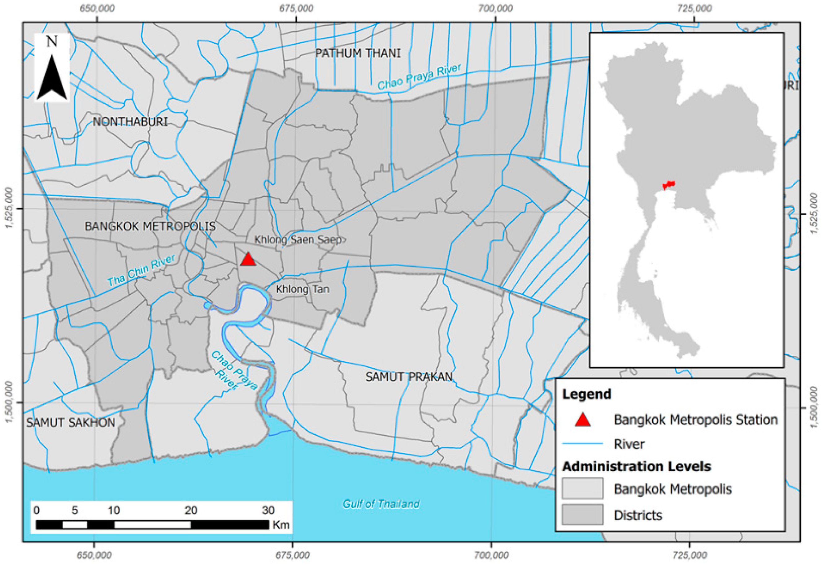
3. Case Study Area
4. Methodology
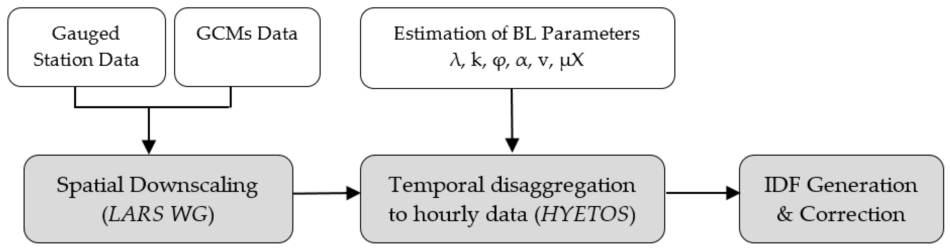
4.1. Methodological Framework for the Spatial Downscaling-Temporal Disaggregation Method (DDM) Approach
4.2. Spatial Downscaling Using Long Ashton Research Station Weather Generator (LARS-WG)
4.3. Disaggregation to Hourly Time Scale Using Hyetos
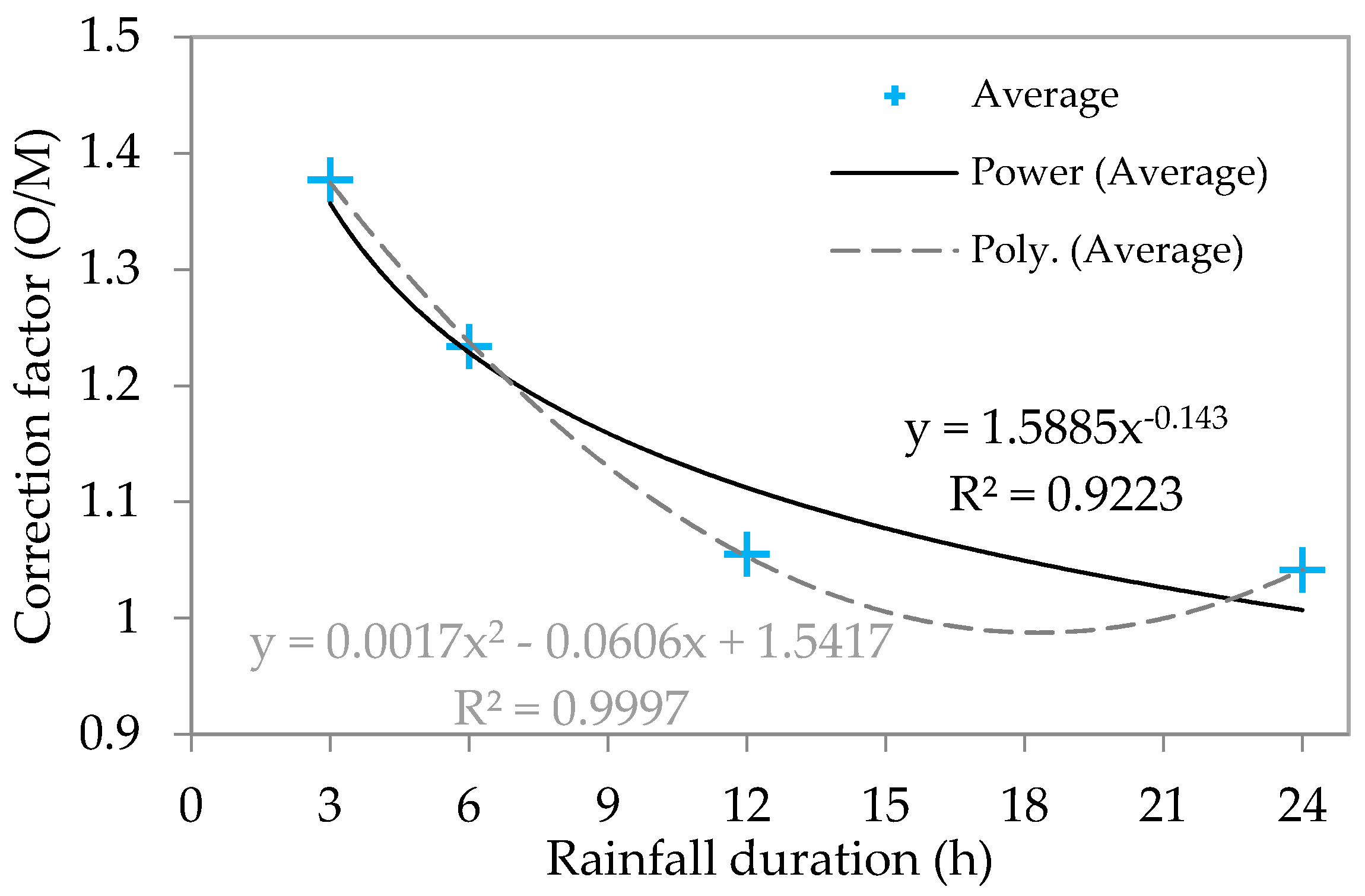
4.4. Intensity–Duration–Frequency (IDF) Generation and Correction
5. Results and Discussion
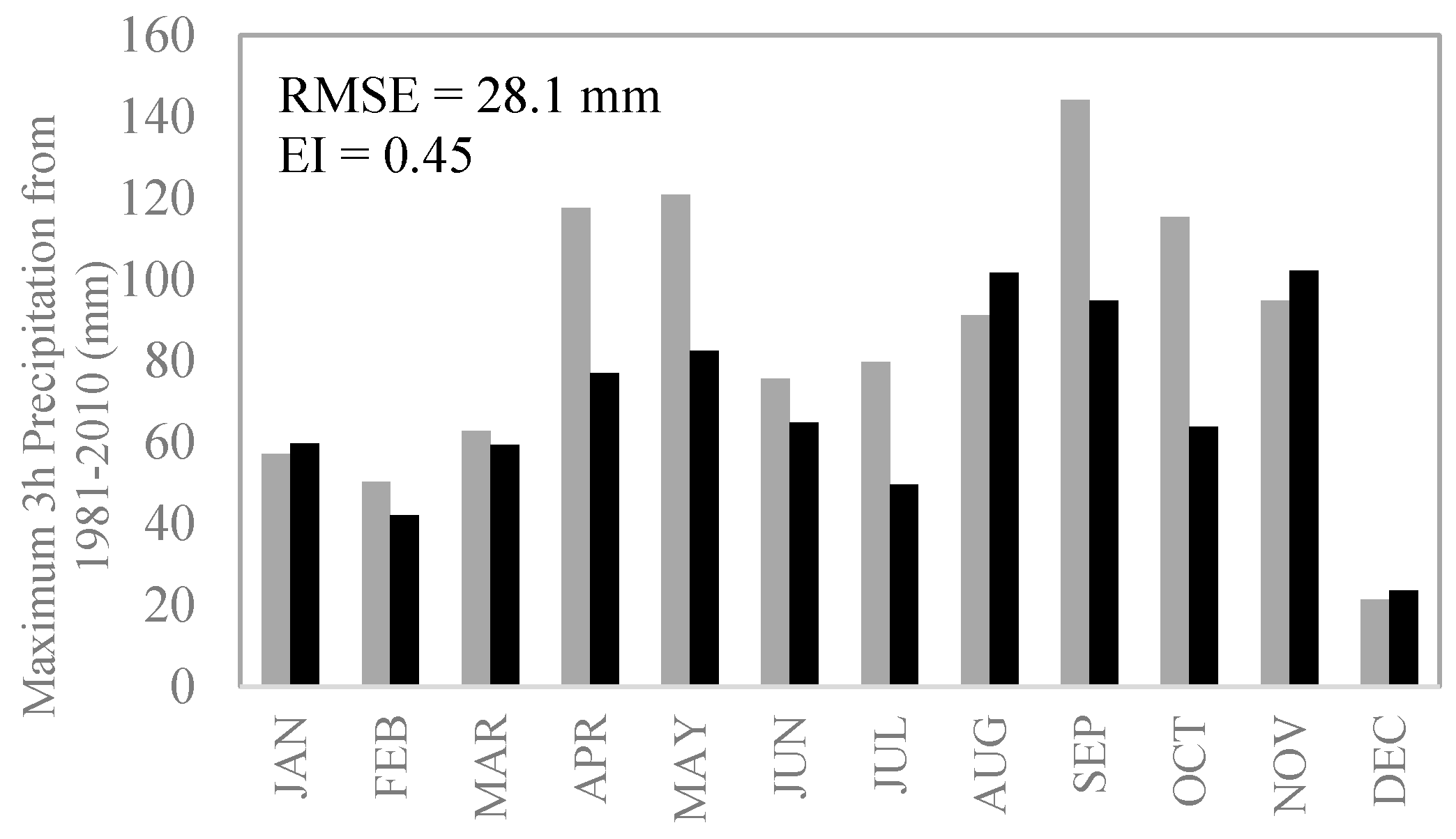
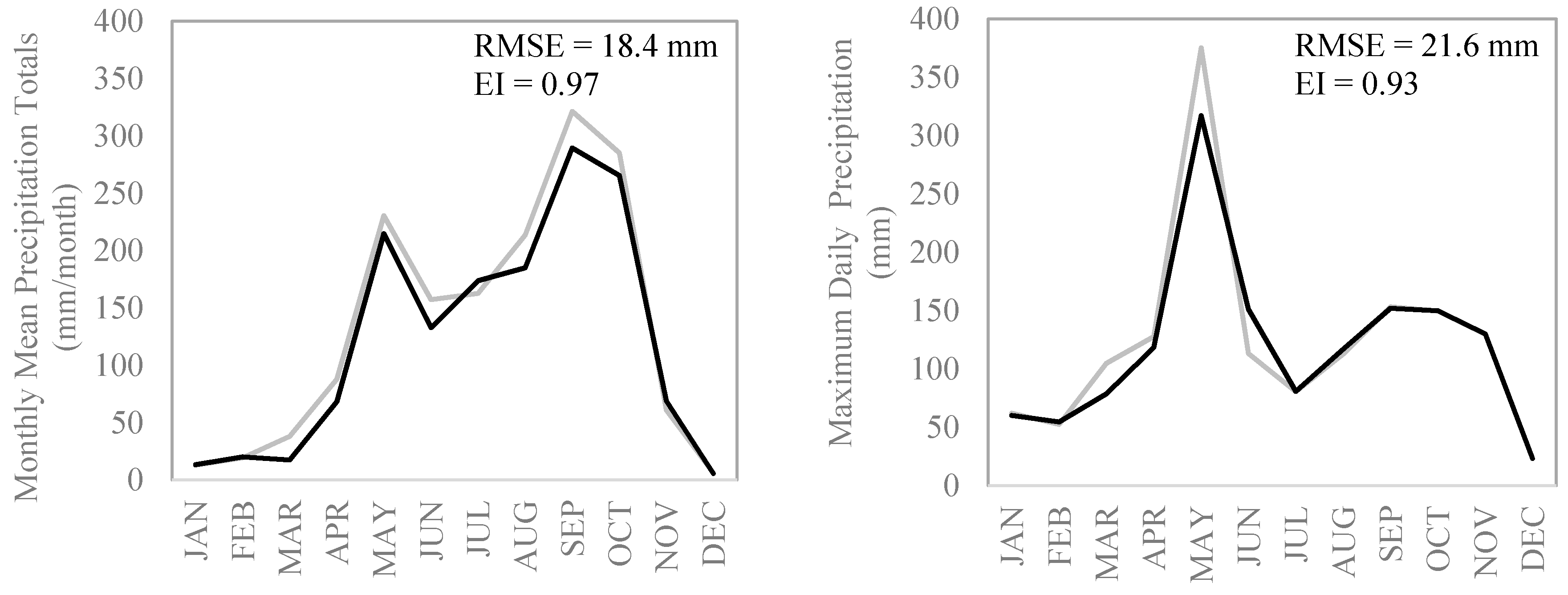
5.1. Spatial Downscaling
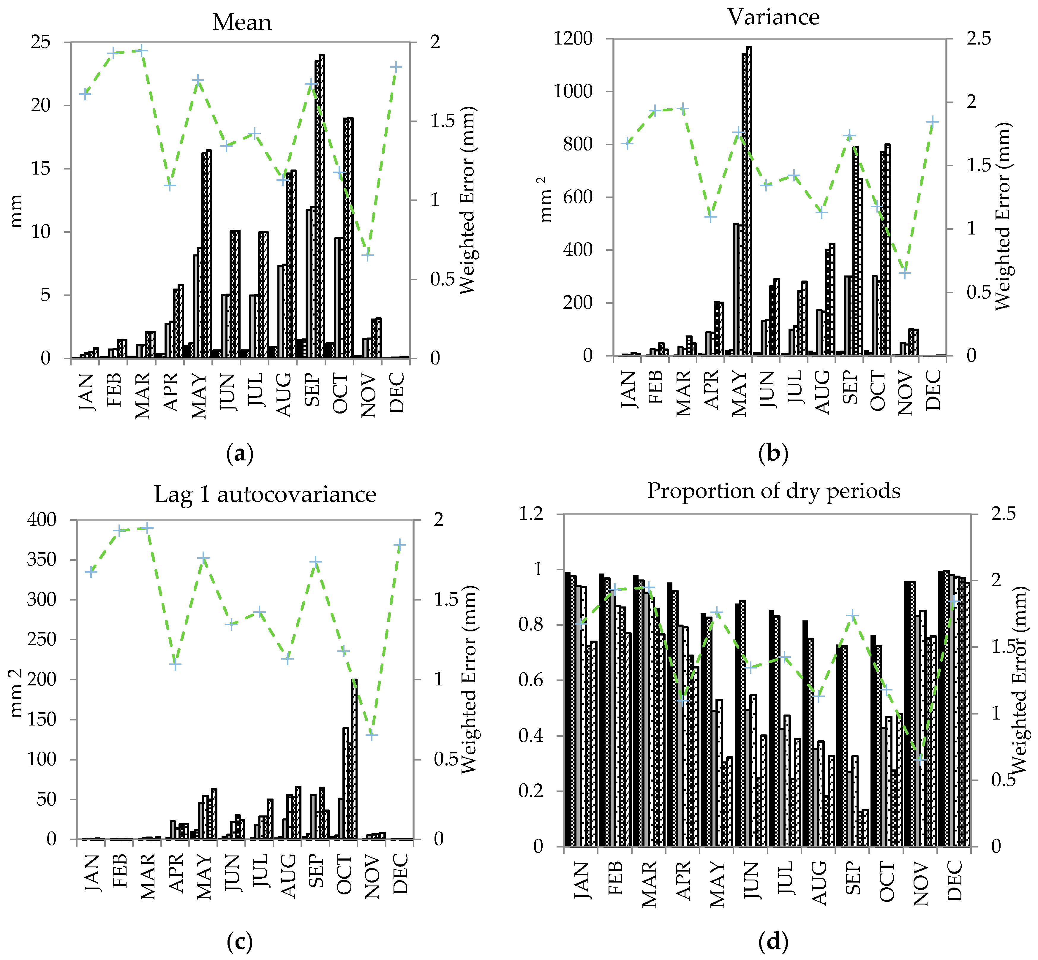
5.2. Temporal Disaggregation
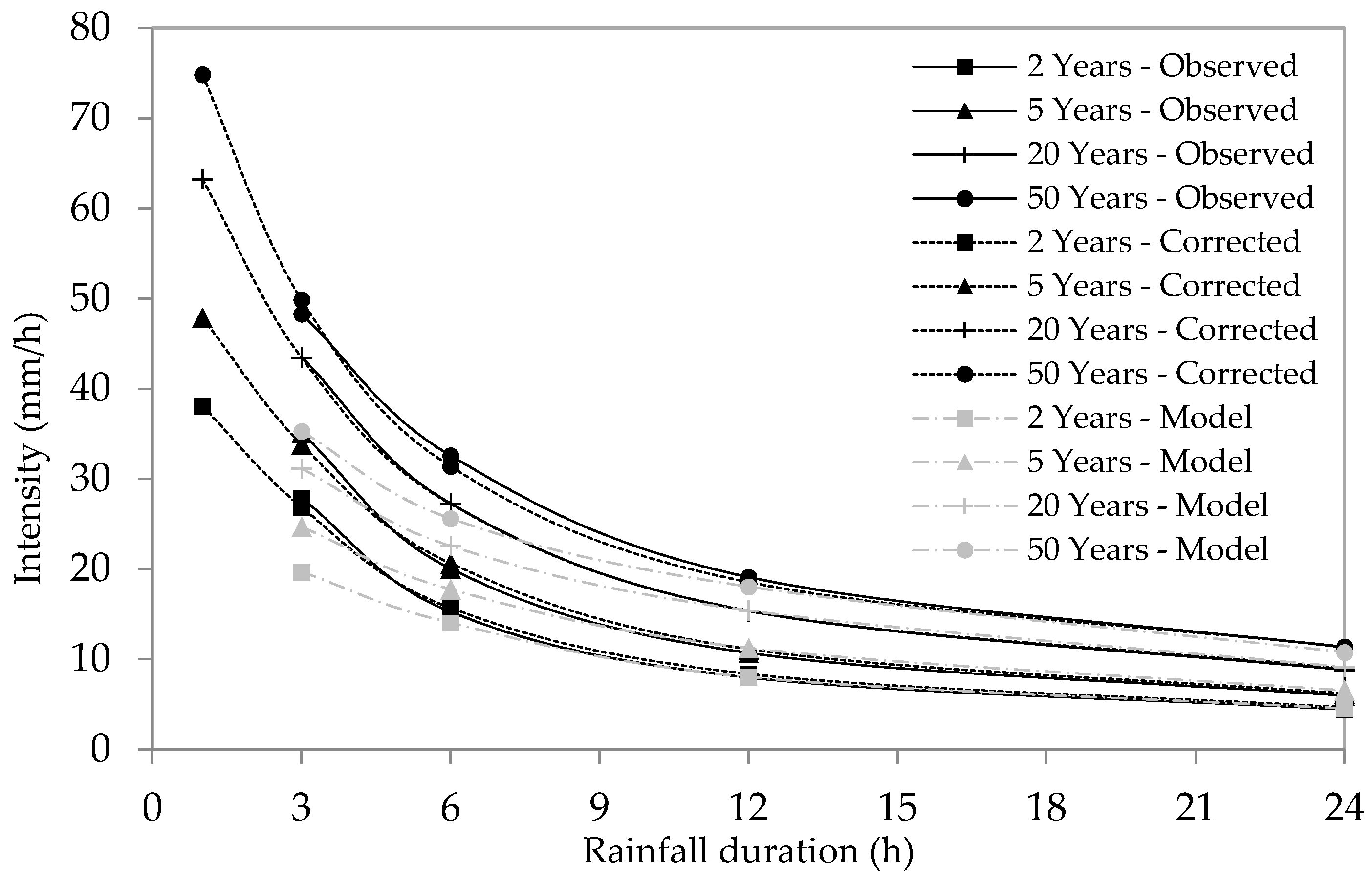
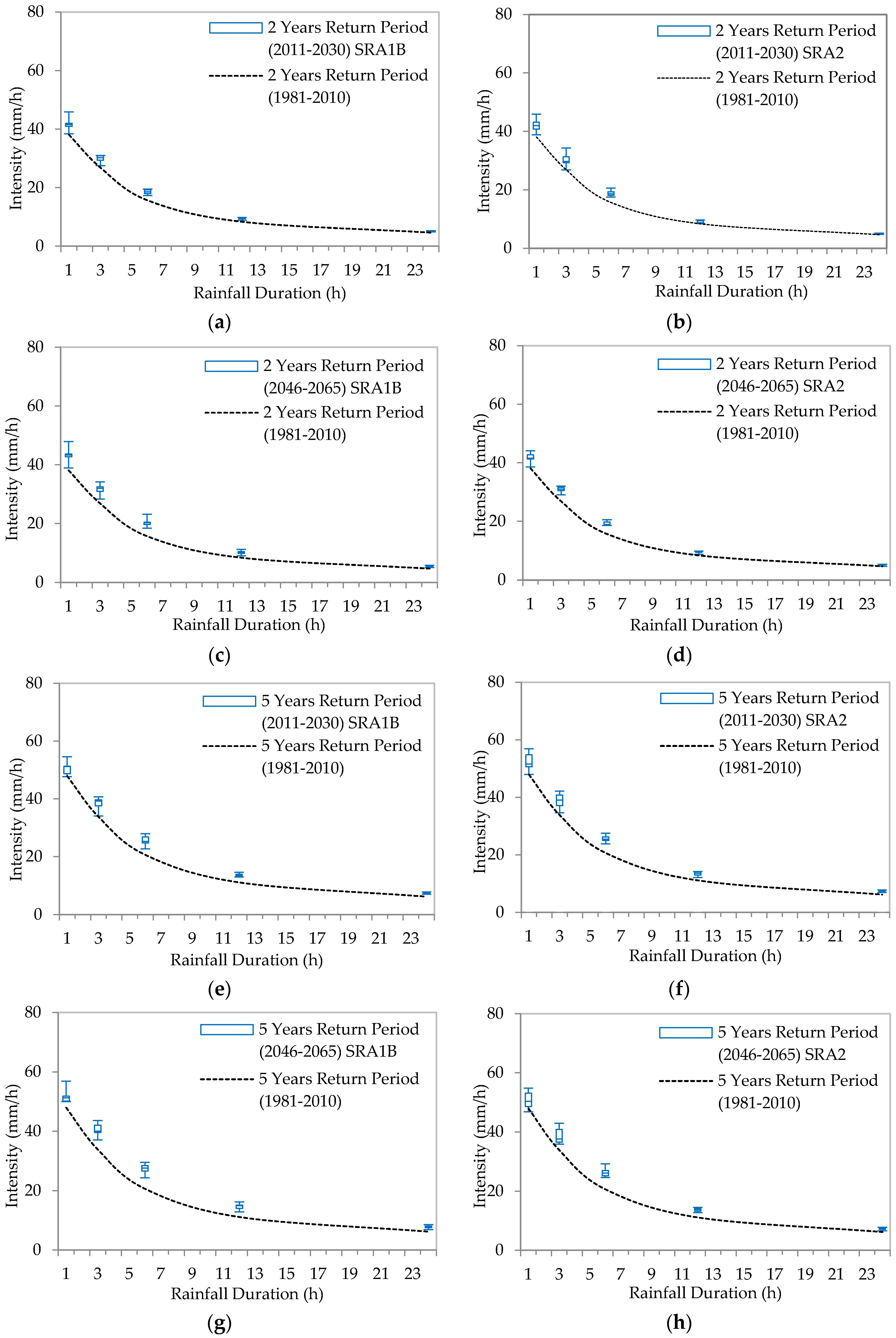
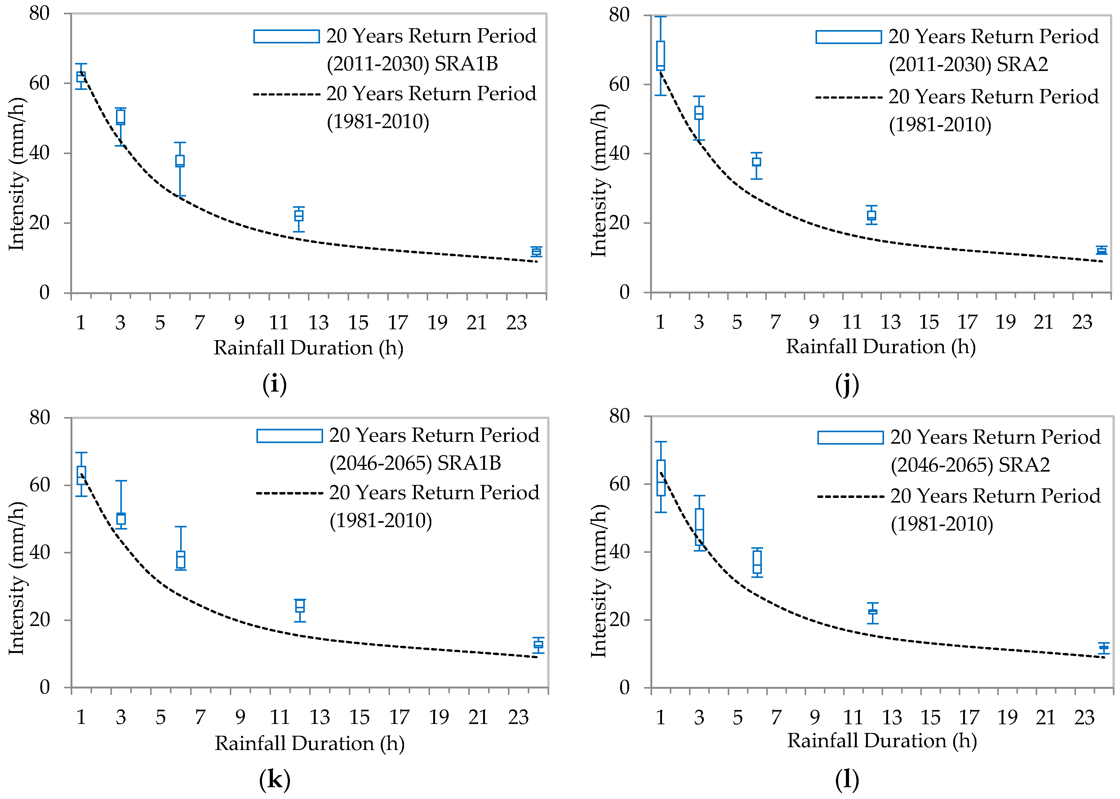
5.3. Generation of IDF Curves
6. Conclusions
Acknowledgments
Author Contributions
Conflicts of Interest
References
- Price, R.K.; Vojinovic, Z. Urban flood disaster management. Urban Water J. 2008, 5, 259–276. [Google Scholar] [CrossRef]
- Mynett, A.E.; Vojinovic, Z. Hydroinformatics in multi-colours—Part red: Urban flood and disaster management. J. Hydroinform. 2009, 11, 166–180. [Google Scholar] [CrossRef]
- Vojinovic, Z.; van Teeffelen, J. An integrated stormwater management approach for small islands in tropical climates. Urban Water J. 2007, 4, 211–231. [Google Scholar] [CrossRef]
- Aerts, J.; Botzen, W.; Bowman, M.; Dircke, P.; Ward, P. Climate Adaptation and Flood Risk in Coastal Cities; Routledge: London, UK, 2013. [Google Scholar]
- Vojinovic, Z.; Sanchez, A.; Barreto, W. Optimising sewer system rehabilitation strategies between flooding, overflow emissions and investment costs. In Proceedings of the 11th International Conference on Urban Drainage, Edinburgh, UK, 31 August–5 September 2008.
- Barreto, W.; Vojinovic, Z.; Price, R.; Solomatine, D. Multiobjective evolutionary approach to rehabilitation of urban drainage systems. J. Water Res. Plan. Manag. 2010, 136, 547–554. [Google Scholar] [CrossRef]
- Vojinovic, Z.; Solomatine, D.; Price, R.K. Dynamic least-cost optimization of wastewater system remedial works requirements. Water Sci. Technol. 2006, 54, 467–475. [Google Scholar] [CrossRef] [PubMed]
- Vojinovic, Z.; Sahlu, S.; Torres, A.S.; Seyoum, S.D.; Anvarifar, F.; Matungulu, H.; Barreto, W.; Savic, D.; Kapelan, Z. Multi-objective rehabilitation of urban drainage systems under uncertainties. J. Hydroinform. 2014, 16, 1044–1061. [Google Scholar] [CrossRef]
- Vojinovic, Z.; Hammond, M.; Golub, D.; Hirunsalee, S.; Weesakul, S.; Meesuk, V.; Medina, N.; Sanchez, A.; Kumara, S.; Abbott, M. Holistic approach to flood risk assessment in areas with cultural heritage: A practical application in Ayutthaya, Thailand. Nat. Hazards 2016, 81, 589–616. [Google Scholar] [CrossRef]
- Alves, A.; Sanchez, A.; Vojinovic, Z.; Seyoum, S.; Babel, M.; Brdjanovic, D. Evolutionary and holistic assessment of green-grey infrastructure for CSO reduction. Water 2016, 8, 402. [Google Scholar] [CrossRef]
- Abbott, M.B.; Vojinovic, Z. Applications of numerical modelling in hydroinformatics. J. Hydroinform. 2009, 11, 308–319. [Google Scholar] [CrossRef]
- Abbott, M.B.; Tumwesigye, B.M.; Vojinovic, Z. The fifth generation of modelling in Hydroinformatics. In Proceedings of the 7th International Conference on Hydroinformatics, Acropolis, Nice, France, 4–8 September 2006.
- Horritt, M.S.; Bates, P.D. Evaluation of 1D and 2D numerical models for predicting river flood inundation. J. Hydrol. 2002, 268, 87–99. [Google Scholar] [CrossRef]
- Hunter, N.M.; Bates, P.D.; Horritt, M.S.; Wilson, M.D. Simple spatially-distributed models for predicting flood inundation: A review. Geomorphology 2007, 90, 208–225. [Google Scholar] [CrossRef]
- Merz, B.; Thieken, A.H.; Gocht, M. Flood risk mapping at the local scale: Concepts and challenges. In Flood Risk Management in Europe; Begum, S., Stive, M.J.F., Hall, J.W., Eds.; Springer: Dordrecht, The Netherlands, 2007; pp. 231–251. [Google Scholar]
- Neal, J.; Villanueva, I.; Wright, N.; Willis, T.; Fewtrell, T.; Bates, P.D. How much physical complexity is needed to model flood inundation? Hydrol. Process. 2012, 26, 2264–2282. [Google Scholar] [CrossRef]
- Panayiotis, D.; Aristoteles, T.; Oikonomou, A.; Pagana, V.; Koukouvinos, A.; Mamassis, N.; Koutsoyiannis, D.; Efstratiadis, A. Comparative evaluation of 1D and quasi-2D hydraulic models based on benchmark and real-world applications for uncertainty assessment in flood mapping. J. Hydrol. 2016, 534, 478–492. [Google Scholar]
- Vojinovic, Z.; Bonillo, B.; Chitranjan, K.; Price, R. Modelling flow transitions at street junctions with 1D and 2D models. In Proceedings of the 7th International Conference on Hydroinformatics, Acropolis, Nice, France, 4–8 September 2006.
- Syme, W. Flooding in urban areas—2D modelling approaches for buildings and fences. In Proceedings of the 9th National Conference on Hydraulics in Water Engineering, Darwin Convention Centre, Darwin City, Australia, 23–26 September 2008.
- Abdullah, A.; Rahman, A.; Vojinovic, Z. LiDAR filtering algorithms for urban flood application: Review on current algorithms and filters test. In Proceedings of the Laserscanning09, Paris, France, 1–2 September 2009; Volume 38, pp. 30–36.
- Vojinovic, Z.; Tutulic, D. On the use of 1D and coupled 1D-2D approaches for assessment of flood damages in urban areas. Urban Water J. 2009, 6, 183–199. [Google Scholar] [CrossRef]
- Seyoum, S.; Vojinovic, Z.; Price, R.K. Urban pluvial flood modeling: Development and application. In Proceedings of the 9th International Conference on Hydroinformatics, Tianjin, China, 7–10 September 2010.
- Evans, B. A Multilayered Approach to Two-Dimensional Urban Flood Modelling. Ph.D. Thesis, University of Exeter, Exeter, UK, 2010. [Google Scholar]
- Abdullah, A.F.; Vojinovic, Z.; Price, R.K. A Methodology for processing raw LiDAR data to support 1D/2D urban flood modelling framework. J. Hydroinform. 2011, 14, 75–92. [Google Scholar] [CrossRef]
- Abdullah, A.F.; Vojinovic, Z.; Price, R.K. Improved methodology for processing raw LiDAR data to support urban flood modelling—Accounting for elevated roads and bridges. J. Hydroinform. 2011, 14, 253–269. [Google Scholar] [CrossRef]
- Vojinovic, Z.; Seyoum, S.D.; Mwalwaka, J.M.; Price, R.K. Effects of model schematization, geometry and parameter values on urban flood modelling. Water Sci. Technol. 2011, 63, 462–467. [Google Scholar] [CrossRef] [PubMed]
- Vojinovic, Z.; Seyoum, S.; Salum, M.H.; Price, R.K.; Fikri, A.F.; Abebe, Y. Modelling floods in urban areas and representation of buildings with a method based on adjusted conveyance and storage characteristics. J. Hydroinform. 2012, 15, 1150–1168. [Google Scholar] [CrossRef]
- Meesuk, V.; Vojinovic, Z.; Mynett, A.; Abdullah, A.F. Urban flood modelling combining top-view LiDAR data with ground-view SfM observations. Adv. Water Resour. 2015, 75, 105–117. [Google Scholar] [CrossRef]
- Sanchez, A.; Medina, N.; Vojinovic, Z.; Price, R. An integrated cellular automata evolutionary-based approach for evaluating future scenarios and the expansion of urban drainage networks. J. Hydroinform. 2014, 16, 319–340. [Google Scholar] [CrossRef]
- Kumar, D.S.; Arya, D.S.; Vojinovic, Z. Modelling of urban growth dynamics and its impact on surface runoff characteristics. Comput. Environ. Urban Syst. 2013, 41, 124–135. [Google Scholar] [CrossRef]
- Singh, R.; Arya, D.S.; Taxak, A.; Vojinovic, Z. Potential impact of climate change on rainfall intensity-duration-frequency curves in Roorkee. Water Resour. Manag. 2016, 30, 4603. [Google Scholar] [CrossRef]
- Trenberth, K.E. Conceptual framework for changes of extremes of the hydrological cycle with climate change. Clim. Chang. 1999, 42, 327–339. [Google Scholar] [CrossRef]
- Trenberth, K.E. Changes in rainfall with climate change. Clim. Res. 2011, 47, 123–138. [Google Scholar] [CrossRef]
- Emori, S.; Brown, S.J. Dynamic and thermodynamic changes in mean and extreme precipitation under changed climate. Geophys. Res. Lett. 2005, 32, L17706. [Google Scholar] [CrossRef]
- Boo, K.O.; Kwon, W.T.; Baek, H.J. Change of extreme events of temperature and precipitation over Korea using regional projection of future climate change. Geophys. Res. Lett. 2006, 33, L01701. [Google Scholar] [CrossRef]
- Koutsoyiannis, D.; Kozonis, D.; Manetas, A. A mathematical framework for studying rainfall intensity-duration-frequency relationships. J. Hydrol. 1998, 206, 118–135. [Google Scholar] [CrossRef]
- Solaiman, T.A.; Siminovic, S.P. Development of Probability Based Intensity-Duration-Frequency Curves under Climate Change; Water Resources Research Report; The University of Western Ontario: London, ON, Canada, 2011. [Google Scholar]
- Mailhot, A.; Duchesne, S. Design criteria of urban drainage infrastructures under climate change. J. Water Resour. Plan. Manag. 2010, 136, 201–208. [Google Scholar] [CrossRef]
- Guo, Y.P. Updating rainfall IDF relationships to maintain urban drainage design standards. J. Hydrol. Eng. 2006, 11, 506–509. [Google Scholar] [CrossRef]
- Rodríguez, R.; Navarro, X.; Casas, M.C.; Ribalaygua, J.; Russo, B.; Pouget, L.; Redaño, A. Influence of climate change on IDF curves for the metropolitan area of Barcelona (Spain). Int. J. Climatol. 2013, 34, 643–654. [Google Scholar] [CrossRef]
- Srivastav, R.K.; Schardong, A.; Simonovic, S.P. Equidistance quantile matching method for updating IDF curves under climate change. Water Resour. Manag. 2014, 28, 2539–2562. [Google Scholar] [CrossRef]
- Nguyen, V.-T.-V.; Nguyen, T.-D.; Cung, A. A statistical approach to downscaling of sub-daily extreme rainfall processes for climate-related impact studies in urban areas. Water Sci. Technol. Water Supply 2007, 7, 183–192. [Google Scholar] [CrossRef]
- Sharma, D.; Gupta, A.D.; Babel, M.S. Spatial disaggregation of bias-corrected GCM precipitation for improved hydrologic simulation: Ping River Basin, Thailand. Hydrol. Earth Syst. Sci. 2007, 11, 1373–1390. [Google Scholar] [CrossRef]
- Piani, C.; Weedon, G.P.; Best, M.; Gomes, S.M.; Viterbo, P.; Hagemann, S.; Haerter, J.O. Statistical Bias Correction of Global Simulated Daily Precipitation and Temperature for the Application of Hydrological Models. J. Hydrol. 2010, 395, 199–215. [Google Scholar] [CrossRef]
- Piani, C.; Haerter, J.O.; Coppola, E. Statistical bias correction for daily precipitation in regional climate models over Europe. Theory Appl. Climatol. 2010, 99, 187–192. [Google Scholar] [CrossRef]
- Hurkmans, R.T.W.L.; Terink, W.; Uijlenhoet, R.; Torfs, P.J.J.F.; Jacob, D.; Troch, P.A. Changes in streamflow dynamics in the Rhine basin under three highresolution climate scenarios. J. Clim. 2010, 23, 679–699. [Google Scholar] [CrossRef]
- Sunyer, M.A.; Madsen, H.; Ang, P.H. A comparison of different regional climate models and statistical downscaling methods for extreme rainfall estimation under climate change. Atmos. Res. 2012, 103, 119–128. [Google Scholar] [CrossRef]
- Wilby, R.; Dawson, C.; Barrow, E. SDSM—A decision support tool for the assessment of regional climate change impacts. Environ. Model. Softw. 2002, 17, 145–157. [Google Scholar] [CrossRef]
- Semenov, M.A.; Barrow, E.M. Use of a stochastic weather generator in the development of climate change scenarios. Clim. Chang. 1997, 35, 397–414. [Google Scholar] [CrossRef]
- Wilks, D.S.; Wilby, R.L. The weather generation game: A review of stochastic weather models. Prog. Phys. Geogr. 1999, 23, 329–357. [Google Scholar] [CrossRef]
- Semenov, M.A.; Stratonovitch, P. Use of multi-model ensembles from global climate models for impact assessments of climate change. Clim. Res. 2010, 41, 1–14. [Google Scholar] [CrossRef]
- Intergovernmental Panel on Climate Change (IPCC). Climate Change 2014: Synthesis Report; Core Writing Team, Pachauri, R.K., Meyer, L.A., Eds.; Contribution of Working Groups I, II and III to the Fifth Assessment Report of the Intergovernmental Panel on Climate Change; IPCC: Geneva, Switzerland, 2014. [Google Scholar]
- Intergovernmental Panel on Climate Change (IPCC). IPCC Special Report Emissions Scenarios; Intergovernmental Panel on Climate Change, Working Group III; IPCC: Geneva, Switzerland, 2000; ISBN 92-9169-113-5. [Google Scholar]
- Willems, P.; Molnar, P.; Einfalt, T.; Arnbjerg-Nielsen, K.; Onof, C.; Nguyen, V.-T.-V.; Burlando, P. Rainfall in the urban context: Forecasting, risk and climate change. Atmos. Res. 2012, 103, 1–3. [Google Scholar] [CrossRef]
- Arnbjerg-Nielsen, K. Quantification of climate change impacts on extreme precipitationused for design of sewer systems. In Proceedings of the 11th International Conference on Urban Drainage Edinburgh, Scotland, UK, 31 August–5 September 2008.
- Willems, P.; Arnbjerg-Nielsen, K.; Olsson, J.; Nguyen, V.T.V. Climate change impact assessment on urban rainfall extremes and urban drainage: Methods and shortcomings. Atmos. Res. 2012, 103, 106–118. [Google Scholar] [CrossRef]
- Koutsoyiannis, D. Rainfall Disaggregation Methods: Theory and Applications. In Workshop on Statistical and Mathematical Methods for Hydrological Analysis; Sapienza University of Rome: Rome, Italy, 2003. [Google Scholar]
- Gyasi-Agyei, Y.; Mahbub, S.M.P.B. A stochastic model for daily rainfall disaggregation into fine time scale for a large region. J. Hydrol. 2007, 347, 358–370. [Google Scholar] [CrossRef]
- Koutsoyiannis, D.; Onof, C. Rainfall disaggregation using adjusting procedures on a Poisson cluster model. J. Hydrol. 2001, 246, 109–122. [Google Scholar] [CrossRef]
- Kossieris, P.; Makropoulos, C.; Onof, C.; Koutsoyiannis, D. A rainfall disaggregation scheme for sub-hourly time scales: Coupling a Bartlett-Lewis based model with adjusting procedures. J. Hydrol. 2016. [Google Scholar] [CrossRef]
- Liew, S.C.; Raghavan, S.V.; Liong, S.-Y. How to construct future IDF curves, under changing climate, for sites with scarce rainfall records? Hydrol Process. 2013, 28, 3276–3287. [Google Scholar] [CrossRef]
- Shrestha, A. Impact of Climate Change on Urban Flooding in Sukhumvit Area of Bangkok. Master’s Thesis, Asian Institute of Technology, Khlong Nung, Thailand, 2013. [Google Scholar]
- Organization for Economic Co-Operation and Development (OECD). Ranking of the World’s Cities Most Exposed to Coastal Flooding Today and in the Future. 2007. Available online: http://www.oecd.org/env/cc/39721444.pdf (accessed on 15 February 2017).
- Klongvessa, P.; Chotpantarat, S. Statistical analysis of rainfall variations in the Bangkok urban area, Thailand. Arab. J. Geosci. 2015, 8, 4207–4219. [Google Scholar] [CrossRef]
- World Bank. Climate Change Impact and Adaptation Study for Bangkok Metropolitan Region; Panya Consultants Co. Ltd.: Bangkok, Thailand, 2009; pp. 1–85. [Google Scholar]
- Chow, V.T.; Maidment, D.R.; Mays, L.W. Applied Hydrology; McGraw-Hill Book Company: New York, NY, USA, 1988. [Google Scholar]
- Hosking, J.R.M. L-moments: Analysis and estimation of distributions using linear combinations of order statistics. J. R. Stat. Soc. B 1990, 52, 105–124. [Google Scholar]
- Hosking, J.R.M.; Wallis, J.R. Regional Frequency Analysis: An Approach Based on L-Moments; Cambridge University Press: New York, NY, USA, 1997. [Google Scholar]


| Model | Research Center | Grid Resolution | Scenarios |
|---|---|---|---|
| CNCM3 | Centre National de Recherches Meteorologiques, France | 1.9° × 1.9° | SRA1B, SRA2 |
| GFCM21 | Geophysical Fluid Dynamics Laboratory, USA | 2.0° × 2.5° | SRA1B, SRB1, SRA2 |
| HADCM3 | UK Meteorological Office, UK | 2.5° × 3.75° | SRA1B, SRB1, SRA2 |
| HADGEM | UK Meteorological Office, UK | 1.3° × 1.9° | SRA1B, SRA2 |
| INCM3 | Institute for Numerical Mathematics, Russia | 4.0° × 5.0° | SRA1B, SRB1, SRA2 |
| IPCM4 | Institute Pierre Simon Laplace, France | 2.5° × 3.75° | SRA1B, SRB1, SRA2 |
| MPEH5 | Max-Planck Institute for Meteorology, Germany | 1.9° × 1.9° | SRA1B, SRB1, SRA2 |
| NCCCSM | National Centre for Atmospheric Research, USA | 1.4° × 1.4° | SRA1B, SRB1, SRA2 |
| NCPCM | National Centre for Atmospheric Research, USA | 2.8° × 2.8° | SRA1B, SRA2 |
| Month | λ (day−1) | Κ = β/η (−) | Φ = γ/η (−) | α (−) | ν (day) | μX (mm·day−1) | σX (mm·day−1) |
|---|---|---|---|---|---|---|---|
| January | 0.1190 | 0.0260 | 0.0227 | 69 | 1.500 | 70 | 70 |
| February | 0.1200 | 0.2400 | 0.1500 | 69 | 2.300 | 70 | 70 |
| March | 0.1150 | 0.1700 | 0.0900 | 86 | 3.200 | 85 | 85 |
| April | 0.1900 | 0.1750 | 0.0910 | 65 | 3.690 | 90 | 90 |
| May | 0.3000 | 0.2500 | 0.0910 | 40 | 3.770 | 90 | 90 |
| June | 0.4100 | 0.4500 | 0.1250 | 69 | 2.600 | 70 | 70 |
| July | 0.2900 | 0.1430 | 0.0330 | 69 | 2.450 | 90 | 90 |
| August | 0.2350 | 0.1360 | 0.0150 | 69 | 2.300 | 90 | 90 |
| September | 0.9000 | 0.6640 | 0.1150 | 90 | 2.500 | 70 | 70 |
| October | 0.1620 | 0.3150 | 0.0150 | 69 | 2.560 | 70 | 70 |
| November | 0.1150 | 0.1900 | 0.0900 | 95 | 4.387 | 95 | 95 |
| December | 0.0240 | 0.1826 | 0.1590 | 100 | 1.960 | 69 | 69 |
| Duration | Distribution | Parameters | K-S Test | χ2 Test | Intensity (mm/h) at Return Periods: | ||||
|---|---|---|---|---|---|---|---|---|---|
| Statistic | p | Statistic | p | 2 Years | 5 Years | 20 Years | |||
| 3 h | GEV | k = 0.08325, µ = 20.652, σ = 76.138 | 0.098 | 0.899 | 2.013 | 0.570 | 27.86 | 35.09 | 43.49 |
| Gamma | α = 13.698, β = 6.3132, γ = 0 | 0.102 | 0.869 | 1.383 | 0.709 | 28.13 | 35.09 | 42.72 | |
| Gumbel | α = 18.218, µ = 75.962 | 0.119 | 0.725 | 3.739 | 0.291 | 27.55 | 34.43 | 43.36 | |
| Log Pearson III | α = 1518.3, β = 0.00689, γ = −6.0309 | 0.106 | 0.842 | 2.206 | 0.531 | 27.78 | 35.05 | 43.69 | |
| Log Normal | α = 0.26397, µ = 4.4251, γ = 0 | 0.110 | 0.807 | 2.226 | 0.527 | 27.84 | 34.77 | 42.98 | |
| Standard Deviation | 0.21 | 0.29 | 0.39 | ||||||
| 6 h | GEV | k = 0.12065, µ = 22.557, σ = 83.159 | 0.079 | 0.982 | 0.358 | 0.949 | 15.27 | 20.04 | 27.29 |
| Gamma | α = 8.8257, β = 11.241, γ = 0 | 0.116 | 0.751 | 1.297 | 0.730 | 15.92 | 20.95 | 26.63 | |
| Gumbel | α = 26.039, µ = 84.183 | 0.093 | 0.926 | 0.119 | 0.998 | 15.62 | 20.54 | 26.92 | |
| Log Pearson III | α = 11.027, β = 0.09135, γ = 3.5429 | 0.085 | 0.966 | 0.345 | 0.951 | 15.30 | 20.10 | 27.21 | |
| Log Normal | α = 0.29842, µ = 4.5502, γ = 0 | 0.105 | 0.848 | 0.145 | 0.997 | 15.78 | 20.28 | 25.77 | |
| Standard Deviation | 0.29 | 0.37 | 0.61 | ||||||
| 12 h | GEV | k = 0.20531, µ = 23.843, σ = 86.68 | 0.135 | 0.581 | 0.475 | 0.924 | 7.98 | 10.71 | 15.35 |
| Gamma | α = 5.3666, β = 19.836, γ = 0 | 0.179 | 0.241 | 7.317 | 0.026 | 8.33 | 11.83 | 15.96 | |
| Gumbel | α = 35.828, µ = 85.771 | 0.164 | 0.335 | 3.010 | 0.390 | 8.24 | 11.63 | 16.02 | |
| Log Pearson III | α = 3.2755, β = 0.18536, γ = 3.9984 | 0.157 | 0.386 | 0.874 | 0.832 | 7.85 | 10.70 | 15.74 | |
| Log Normal | α = 0.33002, µ = 4.6056, γ = 0 | 0.127 | 0.657 | 1.005 | 0.800 | 8.34 | 11.01 | 14.35 | |
| Standard Deviation | 0.22 | 0.52 | 0.69 | ||||||
| 24 h | GEV | k = 0.28101, µ = 24.575, σ = 97.168 | 0.107 | 0.835 | 0.542 | 0.763 | 4.44 | 5.96 | 8.80 |
| Gamma | α = 4.7342, β = 25.493, γ = 0 | 0.192 | 0.180 | 8.616 | 0.035 | 4.68 | 6.80 | 9.33 | |
| Gumbel | α = 43.249, µ = 95.726 | 0.183 | 0.224 | 5.639 | 0.131 | 4.65 | 6.69 | 9.34 | |
| Log Pearson III | α = 2.0027, β = 0.23836, γ = 4.2507 | 0.126 | 0.661 | 3.161 | 0.293 | 4.36 | 5.97 | 9.07 | |
| Log Normal | α = 0.33184, µ = 4.7281, γ = 0 | 0.121 | 0.707 | 1.205 | 0.752 | 4.71 | 6.23 | 8.13 | |
| Standard Deviation | 0.16 | 0.40 | 0.50 | ||||||
| Duration | Comparison * | Return Period | |||||
|---|---|---|---|---|---|---|---|
| 2 Years | 5 Years | 10 Years | 20 Years | 50 Years | 100 Years | ||
| 3 h | Ratio = O/M | 1.426 | 1.426 | 1.406 | 1.377 | 1.332 | 1.295 |
| Difference (mm/h) = O − M | 8.327 | 10.483 | 11.399 | 11.908 | 12.050 | 11.783 | |
| 6 h | Ratio = O/M | 1.047 | 1.093 | 1.159 | 1.242 | 1.373 | 1.489 |
| Difference (mm/h) = O − M | 0.684 | 1.705 | 3.235 | 5.310 | 8.858 | 12.147 | |
| 12 h | Ratio = O/M | 1.007 | 1.020 | 1.036 | 1.057 | 1.090 | 1.119 |
| Difference (mm/h) = O − M | 0.058 | 0.208 | 0.453 | 0.832 | 1.585 | 2.393 | |
| 24 h | Ratio = O/M | 1.013 | 1.025 | 1.035 | 1.045 | 1.060 | 1.072 |
| Difference (mm/h) = O − M | 0.055 | 0.144 | 0.243 | 0.380 | 0.642 | 0.922 | |
| GCMs | Future Period | Scenario | Return Period 2 Years Duration (h) | Return Period 5 Years Duration (h) | Return Period 20 Years Duration (h) | ||||||||||||
|---|---|---|---|---|---|---|---|---|---|---|---|---|---|---|---|---|---|
| 1 | 3 | 6 | 12 | 24 | 1 | 3 | 6 | 12 | 24 | 1 | 3 | 6 | 12 | 24 | |||
| CNCM3 | I | SRA2 | 4.9 | 8.9 | 19.0 | 11.3 | 10.3 | 5.6 | 9.6 | 23.0 | 19.8 | 20.2 | 8.5 | 15.2 | 34.6 | 37.8 | 31.2 |
| SRA1B | 9.0 | 9.4 | 18.2 | 11.9 | 7.5 | 6.9 | 11.1 | 22.2 | 24.8 | 17.9 | 0.1 | 11.3 | 34.7 | 52.7 | 32.9 | ||
| II | SRA2 | 9.0 | 15.4 | 28.7 | 16.6 | 11.4 | 6.9 | 16.6 | 34.0 | 27.6 | 21.9 | 0.8 | 21.4 | 49.6 | 54.9 | 37.9 | |
| SRA1B | 7.3 | 5.4 | 16.9 | 6.7 | 7.7 | 8.2 | 9.6 | 18.0 | 17.1 | 16.7 | 6.0 | 18.9 | 30.2 | 45.8 | 31.9 | ||
| GFCM21 | I | SRA2 | 6.9 | 10.4 | 24.9 | 13.7 | 6.3 | 1.6 | 9.4 | 27.6 | 26.5 | 14.7 | −10.1 | 1.3 | 25.0 | 39.8 | 22.7 |
| SRA1B | 0.8 | 12.6 | 24.4 | 12.5 | 5.7 | −0.2 | 17.2 | 29.8 | 21.3 | 14.1 | 3.7 | 18.4 | 32.8 | 33.1 | 23.1 | ||
| II | SRA2 | 12.0 | 17.6 | 30.6 | 16.3 | 10.5 | 13.2 | 26.7 | 41.7 | 30.6 | 20.4 | 6.0 | 28.9 | 51.2 | 49.2 | 29.3 | |
| SRA1B | 14.6 | 18.4 | 25.1 | 17.1 | 15.4 | 6.9 | 18.1 | 29.0 | 26.2 | 24.7 | −4.8 | 14.9 | 41.3 | 43.6 | 29.7 | ||
| HADCM3 | I | SRA2 | 13.2 | 16.5 | 18.9 | 12.1 | 10.7 | 14.3 | 20.5 | 27.0 | 27.2 | 25.4 | 14.5 | 30.4 | 47.9 | 62.5 | 47.5 |
| SRA1B | 10.1 | 15.4 | 22.9 | 16.8 | 13.0 | 6.9 | 20.4 | 35.2 | 30.9 | 26.4 | −1.5 | 21.9 | 58.1 | 59.8 | 46.3 | ||
| II | SRA2 | 13.2 | 16.5 | 18.9 | 12.1 | 10.7 | 14.3 | 20.5 | 27.0 | 27.2 | 25.4 | 14.5 | 30.4 | 47.9 | 62.5 | 47.5 | |
| SRA1B | 13.6 | 20.8 | 29.9 | 19.2 | 16.6 | 4.6 | 17.0 | 34.0 | 36.1 | 30.8 | −10.2 | 8.5 | 42.5 | 69.8 | 51.2 | ||
| HADGEM | I | SRA2 | 1.8 | -0.1 | 11.4 | 1.1 | 1.6 | 0.0 | 2.2 | 17.6 | 8.9 | 12.3 | 1.3 | 18.9 | 34.9 | 27.8 | 28.4 |
| SRA1B | 7.5 | 2.4 | 10.2 | 9.1 | 5.9 | 1.6 | 3.6 | 19.8 | 19.4 | 16.2 | −4.4 | 11.0 | 39.9 | 42.8 | 29.0 | ||
| II | SRA2 | 4.5 | 11.1 | 26.0 | 11.9 | 9.9 | −2.3 | 5.9 | 26.4 | 23.6 | 21.4 | −18.3 | −7.0 | 19.7 | 41.7 | 31.1 | |
| SRA1B | 12.0 | 27.0 | 47.5 | 33.3 | 22.5 | 7.9 | 24.7 | 43.0 | 45.6 | 34.9 | −1.4 | 18.8 | 28.0 | 50.9 | 40.6 | ||
| IMCM3 | I | SRA2 | 20.4 | 21.2 | 23.1 | 11.7 | 3.8 | 18.7 | 22.9 | 24.7 | 22.0 | 12.6 | 14.8 | 23.6 | 42.0 | 51.9 | 32.1 |
| SRA1B | 10.1 | 15.4 | 22.9 | 16.8 | 13.0 | 6.9 | 20.4 | 35.2 | 30.9 | 26.4 | −1.5 | 21.9 | 58.1 | 59.8 | 46.3 | ||
| II | SRA2 | 15.7 | 17.6 | 20.0 | 12.6 | 9.6 | 5.1 | 9.3 | 20.4 | 19.3 | 17.5 | −10.5 | −3.2 | 25.0 | 40.7 | 30.1 | |
| SRA1B | 13.6 | 20.8 | 29.9 | 19.2 | 16.6 | 4.6 | 17.0 | 34.0 | 36.1 | 30.8 | −10.2 | 8.5 | 42.5 | 69.8 | 51.2 | ||
| IPCM4 | I | SRA2 | 7.2 | 10.4 | 14.3 | 4.1 | 2.2 | 7.4 | 9.6 | 15.1 | 13.0 | 11.2 | 3.3 | 7.1 | 20.0 | 34.3 | 26.7 |
| SRA1B | 2.2 | 5.5 | 14.6 | 13.7 | 10.9 | −0.5 | 0.8 | 9.8 | 16.0 | 16.7 | −5.2 | −3.0 | 2.1 | 14.0 | 16.2 | ||
| II | SRA2 | 8.4 | 14.9 | 20.8 | 10.0 | 5.8 | 1.4 | 11.2 | 24.9 | 21.0 | 14.7 | −10.0 | 7.3 | 32.7 | 48.0 | 31.2 | |
| SRA1B | 2.2 | 15.2 | 28.4 | 24.1 | 16.5 | 4.4 | 24.1 | 40.3 | 34.8 | 26.2 | 10.2 | 41.2 | 75.3 | 56.4 | 37.9 | ||
| MPEH5 | I | SRA2 | 10.1 | 12.6 | 15.5 | 4.1 | 3.9 | 7.7 | 15.3 | 21.0 | 16.6 | 18.1 | 0.9 | 18.7 | 36.8 | 43.2 | 40.1 |
| SRA1B | 11.6 | 12.1 | 13.5 | 6.0 | 3.8 | 8.8 | 16.5 | 21.3 | 18.4 | 17.4 | 0.0 | 20.3 | 44.4 | 45.0 | 39.6 | ||
| II | SRA2 | 10.6 | 19.1 | 19.6 | 3.4 | −1.0 | 10.8 | 21.7 | 30.5 | 14.5 | 7.1 | 11.1 | 16.6 | 43.1 | 46.4 | 28.2 | |
| SRA1B | 12.4 | 14.7 | 29.0 | 25.8 | 21.5 | 6.9 | 18.3 | 34.5 | 39.2 | 37.8 | −2.7 | 18.0 | 51.0 | 68.4 | 65.0 | ||
| NCCCSM | I | SRA2 | 11.9 | 8.8 | 16.4 | 13.7 | 10.7 | 15.6 | 15.6 | 23.3 | 27.1 | 24.3 | 25.9 | 25.6 | 43.1 | 56.4 | 42.1 |
| SRA1B | 20.4 | 15.1 | 22.1 | 15.5 | 11.7 | 13.9 | 14.0 | 24.9 | 25.3 | 22.9 | −1.6 | 8.6 | 32.9 | 42.7 | 36.9 | ||
| II | SRA2 | 1.3 | 8.1 | 18.6 | 14.9 | 13.9 | 0.6 | 7.9 | 22.0 | 25.5 | 24.8 | −4.3 | 1.0 | 24.0 | 46.6 | 35.6 | |
| SRA1B | 25.6 | 26.0 | 29.5 | 19.9 | 11.6 | 18.7 | 28.8 | 37.8 | 33.1 | 22.6 | 1.5 | 26.3 | 48.1 | 54.4 | 36.8 | ||
| NCPCM | I | SRA2 | 19.9 | 27.8 | 30.9 | 14.8 | 7.2 | 12.8 | 24.4 | 33.0 | 21.9 | 13.6 | 2.3 | 16.6 | 34.3 | 36.2 | 22.7 |
| SRA1B | 7.4 | 14.6 | 16.5 | 12.9 | 9.0 | 2.5 | 16.0 | 15.6 | 19.8 | 15.1 | −7.8 | 12.3 | 20.9 | 34.7 | 19.0 | ||
| II | SRA2 | 8.5 | 13.6 | 23.4 | 12.0 | 9.1 | 1.9 | 6.0 | 19.4 | 15.3 | 13.1 | −13.0 | −4.6 | 19.7 | 23.0 | 12.1 | |
| SRA1B | 15.6 | 19.0 | 21.7 | 10.2 | 7.2 | 13.4 | 19.1 | 25.2 | 15.4 | 11.6 | 3.6 | 11.6 | 28.6 | 27.0 | 14.2 | ||
© 2017 by the authors. Licensee MDPI, Basel, Switzerland. This article is an open access article distributed under the terms and conditions of the Creative Commons Attribution (CC BY) license ( http://creativecommons.org/licenses/by/4.0/).
Share and Cite
Shrestha, A.; Babel, M.S.; Weesakul, S.; Vojinovic, Z. Developing Intensity–Duration–Frequency (IDF) Curves under Climate Change Uncertainty: The Case of Bangkok, Thailand. Water 2017, 9, 145. https://doi.org/10.3390/w9020145
Shrestha A, Babel MS, Weesakul S, Vojinovic Z. Developing Intensity–Duration–Frequency (IDF) Curves under Climate Change Uncertainty: The Case of Bangkok, Thailand. Water. 2017; 9(2):145. https://doi.org/10.3390/w9020145
Chicago/Turabian StyleShrestha, Ashish, Mukand Singh Babel, Sutat Weesakul, and Zoran Vojinovic. 2017. "Developing Intensity–Duration–Frequency (IDF) Curves under Climate Change Uncertainty: The Case of Bangkok, Thailand" Water 9, no. 2: 145. https://doi.org/10.3390/w9020145
APA StyleShrestha, A., Babel, M. S., Weesakul, S., & Vojinovic, Z. (2017). Developing Intensity–Duration–Frequency (IDF) Curves under Climate Change Uncertainty: The Case of Bangkok, Thailand. Water, 9(2), 145. https://doi.org/10.3390/w9020145