Influence of Rainfall Characteristics on Total Suspended Solids in Urban Runoff: A Case Study in Beijing, China

Abstract

An urban rainfall-runoff water quality model was developed to simulate total suspend solids (TSS) using the stormwater management model (SWMM) for a 3.8 ha university campus in Beijing (approximately 76.5% impervious), and calibrated and validated against data from two observed rainfall events (221.2 and 16.6 mm rainfall). Model performance is satisfactory (Nash–Sutcliffe model efficiency 0.8 and 0.72 for flow and 0.74 and 0.51 for TSS concentration, respectively). A series of sensitivity model runs were conducted using the calibrated SWMM to study the influences of rainfall characteristics (rainfall hyetographs, depths and durations) and surface flooding on the TSS concentration in outlet runoff of the catchment. The Pilgrim and Cordery rainfall distribution defines a first-quartile storm (the most severe) and results in the highest peak discharge and TSS concentration at the outlet but the lowest outlet TSS load because of the highest TSS flood loss (32.3%). The simulated TSS pollutograph resulting from the Keifer and Chu rainfall distribution (with r = 0.5) is almost identical to that resulting from the alternating block rainfall distribution. Under the same rainfall hyetograph, simulated peak discharge and outlet TSS load are positively correlated (R² = 0.95) to the rainfall depth as a function of the return period.

1. Introduction

As the point source pollution has been largely controlled, non-point source (NPS) pollution is becoming the main contributor of urban water quality deterioration in China [1,2]. During and after a rainfall event, pollutants are detached (or dissolved) by rainfall–runoff and transported into any nearby water body, resulting in water pollution. Most NPS pollutants enter urban water systems by rainfall-runoff. Danz et al. [3] showed that the majority of the annual sediment and phosphorus loading is delivered to surface waters during rainfall events. Thus, to some degree, urban NPS pollution can be termed “rainfall-runoff pollution”. Therefore, urban rainfall-runoff was listed as the third major pollutant source in the USA [4]. Yoon et al. [5] illustrated that urban NPS pollution is significantly influenced by many factors, among which are rainfall characteristics (rainfall intensity, rainfall duration, and rainfall depth), land use, number and distribution of dry days, and street cleaning methods. The washoff of surface pollutants depends on rainfall intensity, the dilution of pollutants depends on rainfall depth, and the timing of the pollutant washoff process and of pollutant transport depends on rainfall distribution [6].

Total suspended solids (TSS) is a commonly used monitoring indicator of NPS pollution. In this study, TSS is the dry-weight of particles trapped by a 0.45-µm filter and does not include dissolved solids in stormwater. It may include water-insoluble inorganic material (e.g., sediment and clay) and insoluble organic matter (e.g., fecal matter, plankton, vegetation, and microorganisms). For typical stormwater samples, TSS are significantly larger than dissolved solids. All waterbodies contain TSS due to natural processes, but anthropogenic activity results in elevated TSS concentration. Thus, monitoring of TSS concentration is a very good predictor of water quality. Bilotta and Brazier [7] found that elevated concentrations of TSS due to, for example, anthropogenic perturbations, alter the physical, chemical and biological properties of a waterbody.

Moreover, TSS is linked to other pollutants, such as phosphorus, organic compounds, and some heavy metals, since they tend to be adsorbed in particles [8,9,10,11]. More than 80% of adsorbed pollutants are linked to TSS during rainfall events [12]. Herngren et al. [13] found that some heavy metals in water, such as Cu, Pb and Fe, have a close relationship with TSS. In addition, TSS plays an important role in the transport of anthropogenic nutrients and heavy metals in streams [14]. Thus, monitoring TSS in stormwater is an acceptable means by which to assess NPS pollution from urban areas.

Other research has indicated that TSS concentration in urban runoff significantly varies with the rainfall characteristics. Deletic [13] found that the event maximum rainfall intensity and the time of its appearance from the start of the event were the most important parameters for predicting the “first flush” load of TSS. Zhang et al. [14] reported that total rainfall amount is an important factor for urban runoff pollution, but not the only factor; rainfall intensity and the duration of the dry period also greatly influence the pollution load of urban runoff. Understanding the effects of rainfall characteristics on TSS and other pollutants (e.g., volatile organic components) from urban roads or watersheds has been studied using modeling approaches [15,16] and analyzing measurements from runoff produced by rainfall simulators [17].

This study analyzed the effects of rainfall characteristics on TSS in an urban catchment in Beijing, China, where underground stormwater infrastructure was undersized to cause surface flooding. The characteristics examined were the temporal distribution of rainfall (hyetograph), rainfall depth (or intensity) as a function of return period, and rainfall duration under different dry days. The purpose of this paper is to provide technical information of runoff TSS dynamics for better urban NPS pollution control. When the underground stormwater sewer system is under-designed, heavy rainfall events can lead to surface flooding that may not flow back into the pipelines. A series of sensitivity model runs under various design rainfall characteristics are conducted for the study catchment. The case study is to understand how both rainfall characteristics and surface flooding can influence TSS at the outfall of the catchment. The model used for the case study was calibrated and validated using data from two observed rainfall events.

2. Materials and Methods

2.1. Study Area

The study area is located in Beijing, China, which has a sub-humid continental monsoon climate with a mean annual temperature of 12 °C and a mean annual precipitation of 626 mm (80% of which falls from June to September). The study area is a university campus that includes buildings, lawns, and roads, and is relatively flat with a ground elevation difference of 0.5 m. The drainage area of the catchment is 3.8 ha, and approximately 76.5% of the catchment area is impermeable (1.62 ha of roads and 1.29 ha of buildings). The study area was divided into 30 sub-catchments (denoted S1 to S30 in Figure 1) for the stormwater management model (SWMM) model simulation. The areas of the 30 sub-catchments range from 0.03 ha to 0.31 ha. The percentages of roads, buildings, and green areas (lawns) in the 30 sub-catchments range from 8% to 83%, 0% to 76%, and 0% to 63%, respectively. The study area has gentle slopes ranging from 0.2% to 0.66%. There are 30 underground stormwater pipes with junctions (J1 to J30) connecting the 30 sub-catchments to a single outlet (Outfall in Figure 1) in the catchment.

The underground stormwater sewer system was originally designed and constructed in the 1990s, and was remodeled in 2013 to mitigate and alleviate surface flooding in the study area. Surface flooding and inundation occurred in the past, even for common rainfall events of one-year return period. The pipeline diameters, lengths, and longitudinal slopes range from 0.2 m to 0.7 m (most diameters are 0.3 m), from 4.3 m to 83.4 m, and from 0.2% to 1%, respectively.

2.2. Flow Measurement and Stormwater Sampling

Because the outlet of the catchment (Outfall in Figure 1) was not accessible, the monitoring point was set in a manhole at junction J29 (Figure 1). An area-velocity module flow meter [18] to measure water level and flow rate during and after rainfall events was installed in the end of conduit C27 (star in Figure 1) connecting junctions J27 and J29. The water level and flow rate were automatically recorded at an interval of 1 min for wet days and at an interval of 5 min for dry days. Rainfall data were recorded by an automated weather station (Onset’s HOBO) (Figure 1) at an interval of 1 min.

A full-size portable water sampler [19] was used to collect stormwater runoff samples from the conduit C27 (Figure 1) during rainfall events. Then, the TSS concentration of each sample was measured according to the Chinese national criteria (GB 11901-8) [20] using the gravimetric method. Both flow rates and stormwater samples collected at the conduit C27 excluded contributions from sub-catchments S28, S29, and S30 (Figure 1).

2.3. Water Quality Model

The SWMM is a dynamic rainfall–runoff simulation model that can be used for single-event or long-term continuous simulation of runoff quantity and quality from urban areas [21]. SWMM has been widely used for various stormwater modeling studies and was also used for the case study since it is free and available for download even though there are other integrated models such as MIKE URBAN [22] and InfoWorks ICM [23] that can be used and give similar results. Ouyang et al. [19] used the SWMM model to assess the stormwater runoff pollution loading in Beijing and concluded that SWMM could be used to express the stormwater pollution patterns from diverse underlying surfaces.

In the SWMM model, the generation and accumulation of pollutants mainly occur in the absence of rain (i.e., during dry periods). The background TSS concentration is 10 mg/L [21]. Pollutants are removed from surfaces by the washing action of rainfall and runoff. Exponential functions are used to describe the buildup and washoff of pollutants. Pollutant buildup that accumulates within a land use category is described by a mass (kg) per unit of sub-catchment area or curb-length. The amount of buildup B (kg/ha) is a function of the number of antecedent dry days (t) and land use type and is computed using Equation (1) [21]:

$$B=C_1\left(1-e^{-C_{2}t}\right)$$

(1)

where C₁ is the maximum possible buildup (kg/ha) and C₂ is the buildup rate constant (1/day) as function of land use.

The washoff load in units of mass per hour is proportional to the product of runoff raised to some power and to the amount of buildup remaining [19]. Pollutant washoff (W in kg/h) from a given land use category that occurs during wet weather periods is empirically calculated using Equation (2)

$$W_t=C_3{q}_t^{C_4}{B}_T$$

(2)

where C₃ is the washoff coefficient ((mm/h)^−C4·h⁻¹), C₄ is the washoff exponent (dimensionless), q_t is the runoff rate per unit area at time t (mm/h), and B_T is the total mass of pollutant buildup (kg, not per area or per curb length) remaining on the surface at time t.

2.4. Model Calibration and Validation

TSS is a common pollutant in urban stormwater runoff. Using TSS as an indicator, urban NPS pollution in the study area was simulated using the SWMM model under different rainfall patterns after the SWMM model was calibrated and validated using observed data.

The SWMM model developed for the study area was calibrated and validated against observed data from two rainfall events: 21 July 2012 (calibration) and 7 June 2013 (validation). The monitoring point (Figure 1) was not accessible for additional monitoring after June 2013 due to a construction project. Beijing is an arid area with fewer rainfall events each year; therefore, only these two rainfall events were finally available for model calibration and validation. The total rainfall depths, durations, and maximum rainfall intensities of the two rainfall events are summarized in

Table 1. Summary of rainfall characteristics and hydrographs for two rainfall events for model calibration and validation.

Events/Parameters	Total Rainfall Depths (mm)	Duration of Rainfall (min)	Peak Rainfall (mm/h) and Time (h:min)	Cumulative Runoff Volume (C27, m3)	Peak Discharge (C27, L/s)
21 July 2012	221.2	935	2 (14:24)	2444.6 (3135.1) 1	266.0 (249.3) 1
7 June 2013	16.6	312	0.6 (8:56)	376.3 (234.2) 1	127.0 (125.3) 1

Note: ¹ The first number is observed value, and the number inside brackets is corresponding simulated values.

. The rainfall on 21 July 2012 was very high with an approximate return period of 20–50 years and resulted in flooding and inundation in various areas in Beijing [24]. Thus, using observed flow and pollutant data, model parameters, Manning’s coefficients and depression storages for pervious and impervious areas, and C₁, C₂, C₃, and C₄ for Equations (1) and (2) of the SWMM model, were calibrated and validated for a quite severe event and a relatively light rainfall event (Table 1), respectively.

In this study, the SWMM performance was evaluated on the basis of the Nash–Sutcliffe efficiency coefficient (E_NS) [25] and absolute relative error (RE), which are goodness-of-fit criteria for comparing the simulated and observed values. E_NS value ranges from −∞ to 1, and scientists generally recognize that E_NS values exceeding 0.7 suggest that the simulated results have a good agreement with observed data [26]. Likewise, RE values between 0% and 25% show that the SWMM model reasonably well represents flow and water quality processes in the study area.

2.5. Design Rainfall

In this study, the effects of rainfall characteristics such as duration (D, in min), depth (mm) as function of return period (T_r, in year), and rainfall distribution over time (as described using a hyetograph) on urban NPS pollution (as indicated by TSS) were investigated using different types of design rainfall events. The design rainfall intensities and depths were calculated according to the rainfall intensity–duration–frequency (IDF) equations for Beijing:

$$i=\frac{12.0(1+0.811{log}_{10}{T}_r)}{{\left(D+8\right)}^{0.711}}\mathrm{for}D\le 120\min$$

(3)

$$i=\frac{13.9(1+1.091{log}_{10}{T}_r)}{{\left(D+10\right)}^{0.759}}\mathrm{for}120\min <D\le 360\min$$

(4)

where i is average rainfall intensity (mm/min). The return period T_r is less than 10 years for Equations (3) and (4). Total rainfall depth is the average rainfall intensity i multiplied by the duration D (min) of the design storm.

2.5.1. Rainfall Hyetograph

After the design storm depth and duration were established, a representative hyetograph has to be selected to distribute the design rainfall over time. To examine the effects of time distribution (rainfall pattern) on flow rate and TSS at the outlet of the watershed, three hyetographs (Figure 2) were used initially to perform the sensitivity analysis (or scenario model runs). The first hyetograph was a hypothetical uniform rainfall pattern using i calculated from Equations (3) and (4). The second hyetograph was calculated using the method proposed by Keifer and Chu [27], and resulted in a hyetograph that subsequently is called the “K&C distribution” of Beijing design storm in this paper.

Keifer and Chu [27] originally applied and tested the method using the IDF curve for Chicago, USA, and the method since then has been applied globally in many other cities. In addition to a local IDF curve, the K&C method uses one parameter r (0 < r < 1.0) to represent the portion of rainfall that occurs over the duration prior to the most intense rainfall moment. Keifer and Chu [27] determined an average r = 0.375 from 27 rainfall events in Chicago. The value of r ranged from 0.31 to 0.49 when the K&C method was applied to five cities in the USA. In this study, we used three r values (0.375, 0.5, and 0.75) to generate three K&C distributions (Figure 3) for the sensitivity analysis. Qin et al. [28] used nine r values between 0.1 and 0.9 with 0.1 increment for K&C distributions to study the impact of rainfall hyetograph on runoff hydrograph.

The third hyetograph was calculated using the method proposed by Pilgrim and Cordery [29], subsequently called the “P&C distribution” in this paper (Figure 2). The P&C method was designed to overcome the problem of missing time sequences of intensities, and used rainfall data of the same duration (including intense bursts) that were typically used to develop IDF curves. Neither the P&C method nor the K&C method use the rainfall pattern of complete storms, in contrast to other methods, e.g., Hershfield [30], Huff [31], Pani and Haragan [32], and Asquith, et al. [33].Mou [34] applied the P&C method to long-term heavy rainfall events in Beijing central districts to derive rainfall distributions for three P&C design storm durations (60, 120, and 180 min). These P&C distributions give the percentage of rain falling in each 5-min interval and are used in this study.

Figure 2 shows three rainfall patterns used in SWMM model simulations for a three-year return period, 2-h duration storm. The total design rainfall depth for the three-year, 2-h event in Beijing is 63.4 mm (Equation (3)). The rainfall occurring in 5-min intervals was used as input for SWMM modeling. For the K&C and P&C distributions, peak 5-min incremental rainfalls are 13.04 mm and 13.83 mm, respectively, and occur at 45–50 min and 20–25 min, respectively (

Table 2. Summary information for design rainfall distributions used in model simulations.

Design Rainfall	Uniform	K&C Distributions					P&C Distributions			Block
Return Period	3 year	1 year 1	3 year 1	5 year 1	3 year 2	3 year 3	3 year	3 year	3 year	3 year
Duration (min)	120	120	120	120	120	120	60	120	180	120
Depth (mm)	63.4	45.8	63.4	71.7	63.4	63.4	49.7	63.4	70.8	63.4
∆Dmax (mm) 4	2.64	9.41	13.04	14.74	10.66	12.34	12.85	13.83	12.45	13.44
imax (mm/h) 5	31.7	112.9	156.5	176.9	127.9	148.1	154.2	166.0	149.4	161.3
Time of imax (min)	-	45 6	45	45	55	85	20	20	30	55

Notes: ¹ The constant r for the standard Keifer and Chu (K&C) method is 0.375; ² for r = 0.5; ³ for r = 0.75; ⁴ ∆D_max is the maximum 5-min incremental rainfall; ⁵ i_max is the maximum 5-min rainfall intensity; ⁶ The rainfall input was for 5-min intervals, and “45” indicates the time of peak rainfall (intensity) occurring in the timespan from 45 to 50 min.

). These rainfall distributions are classified as second- and first-quartile storms based on the location of the storm peak within the distributions [31].

Figure 3 shows rainfall patterns calculated using the Beijing K&C distributions with r = 0.375, 0.5 and 0.75, as well as using the alternating block rainfall distribution, for a three-year 2-h design storms [35]. For r = 0.375, 0.5 and 0.75, the K&C method produces peak 5-min incremental rainfalls of 13.04 mm, 10.66 mm, and 12.34 mm, respectively, which occurs at 45–50 min, 55–65 min (two peaks), and 85–90 min, respectively. The alternating block method is often used in the USA for developing hyetographs for design storms [35], and is similar to the K&C method in that it utilizes average rainfall intensities calculated from a local IDF curve. The highest rainfall is assumed to occur at the mid-point of the design storm duration (13.44 mm at 55–60 min in Figure 3), and the remaining blocks of rainfall are arranged in descending order from the center block to the right and left [36].

2.5.2. Different Return Periods

The 2-h design rainfalls calculated using the K&C method (with r = 0.375) and Equation (3) for one-year, three-year, and five-year return periods are also used for sensitivity analysis. The corresponding total rainfall depths are 45.8 mm and 71.7 mm for one-year and five-year return periods, respectively (Table 2). Peak rainfall for three design storms occurs in 45–50 min (Figure 4 and Table 2).

2.5.3. Rainfall Durations

To further investigate the effects of rainfall duration on TSS in urban runoff, the design rainfall hyetographs for three durations (1 h, 2 h, and 3 h, Figure 5a) of a three-year return period were developed using the P&C method [34]. The 1-h P&C distribution is a second-quartile storm, and the 2- and 3-h P&C distributions are first-quartile storms [31]. The design rainfall hyetographs of K&C distributions for three durations (Figure 5b) of a three-year return period event were also developed. All K&C distributions are classified as second-quartile storms because of the r value of 0.375 that was used. The design rainfall characteristics are summarized in Table 2. Incremental rainfalls in the K&C distributions increases smoothly to the peak values and then gradually decreases, but incremental rainfalls in the P&C distributions changes somewhat irregularly.

3. Results and Discussion

3.1. Model Calibration and Validation Results

Developed SWMM model was calibrated and validated for flow rate (L/s) and TSS concentration (mg/L) at the end of the conduit C27 (Figure 1) using measurements from two rainfall events: 21 July 2012 (Figure 6) and 7 June 2013 (Figure 7), respectively. The number of dry days before the event on 21 July and 7 June were 10 d and 3 d, respectively. The calibrated Manning’s roughness coefficients for underground pipelines, impervious and pervious surfaces were 0.013, 0.011, and 0.15, respectively. Calibrated depression storage for impervious and pervious surfaces was 2 mm and 12 mm, respectively. Horton’s equation [37] was used for infiltration computation of pervious surfaces, resulting in a maximum infiltration rate of 103.81 mm/h, an equilibrium infiltration rate of 11.44 mm/h, and a decay constant of 8.46 h⁻¹.

The heavy rainfall on 21 July 2012 (Table 1) had several intense rainfall periods (bursts) that resulted in multiple discharge peaks. The simulated hydrograph from the SWMM model reproduced these peaks well in both timing and magnitude. The maximum 1-min intensity (2 mm/min) on 21 July occurred at 12:25–12:28, and there was continuous heavy rainfall from 17:50 to 20:00 at an average intensity of 0.82 mm/min (and maximum of 1.8 mm/min). The rainfall on 7 June 2013 had a duration of 4.2 h and a lower rainfall intensity (maximum intensity of 0.58 mm/min), and resulted in one discharge peak of 122 L/s (observed), which was simulated by SWMM to be 125.4 L/s.

In normal flow routing within SWMM, when the flow into a pipeline junction (e.g., a manhole) exceeds the capacity of the system to transport it further downstream, the excess volume of water overflows the system (creating surface flooding and inundation) and is lost from the pipeline system. However, when the “Allow Ponding” option in SWMM is selected, ponded water on the surface is reintroduced into the subsurface system as pipeline capacity permits. Hydrographs for model calibration and validation (Figure 6 and Figure 7) were simulated when the “Allow Ponding” option in SWMM was not active. For the event on 21 July 2012, the system overflow was simulated to start at 13:16 at node J15 and stop at 1:14 on 22 July 2012 at node J16. However, the overflow periods were not continuous, but rather occurred over several discrete time intervals.

The E_NS value of the SWMM model for the conduit discharge at C27 was 0.80 for the calibration event and 0.72 for the validation event, which is evidenced by reasonable agreement between the observed and simulated discharges (Figure 6a and Figure 7a). Simulated discharges could be much larger than observed discharges on 21 July 2012, with E_NS = −0.02 if the “Allow Ponding” option in SWMM was selected to allow ponded water to be reintroduced into the subsurface stormwater drainage system. Therefore, in reality, after the flooding of junctions, runoff stayed in depression areas above ground or flowed outside of the catchment and did not flow back into underground pipelines. On 21 July, 18 nodes (manholes) were flooded for durations ranging from 0.08 h (5 min) to 3.2 h (the total flooding time for all 18 nodes was 26.7 h). Although the event on 7 June 2013 produced relatively small rainfall (Table 1), two nodes (J15 and J16) were flooded for 4–5 min, indicating that the underground pipelines in the catchment were under-designed.

Table 3. Calibrated SWMM model parameters for TSS simulations.

Land Use	C1 (kg/ha) 1	C2 (1/days) 1	C3 2	C4 2
Road	150	0.5	0.012	1.8
Roof	60	0.5	0.007	1.8
Green space	40	0.5	0.004	1.2

Notes: ¹ Coefficients C₁ and C₂ are defined in Equation (1) for sediment buildup. ² Coefficients C₃ and C₄ are defined in Equation (2) for runoff wash-off.

contains calibrated SWMM model parameters that are defined in Equation (1) for sediment buildup and Equation (2) for runoff washoff as function of land use types (road, roof, and green space). Gironas et al. [38] demonstrated the application of SWMM to simulate runoff water quality from a 29-acre (11.7 ha) urban catchment and drainage system. The maximum buildup possible (C₁) was given in imperial units of lbs/curb-mile/day using data from Manning et al. [39], and cannot be compared with C₁ in units of kg/ha as used in this study. The buildup constant C₂ was 0.5/day for residential areas and 0.2/day for commercial areas, and the washoff exponents were 1.8 for residential areas and 2.2 for commercial areas. According to sediment transport theory, C₄ should range between 1.1 and 2.6 [40]. The washoff coefficient C₃ can vary in nature by three or four orders of magnitude; for example, Gironas et al. [38] used 0.059 (mm/h)^−1.8·h⁻¹ for residential areas and 0.032 (mm/h)^−2.2·h⁻¹ for commercial areas (as converted to SI units). Li et al. [41] calibrated SWMM’s water quality parameters using data collected for a roof in the Shanghai area of China and determined C₁ to be 355 kg/ha, C₂ to be 0.4/day, C₄ to be 1.3, and C₃ to 0.074 (mm/h)^−1.3·h⁻¹. In summary, the calibrated model parameters determined in this study and shown in Table 3 are in the range of values reported in the scientific literature.

In the SWMM model, the option to designate removal of sediment from surfaces by sweeping was set as zero for all simulations. In the calibration run for the 21 July 2012 rainfall event, the simulated peak TSS concentration was 900.5 mg/L and occurred at 13:20 (Figure 6b). A second and smaller TSS peak resulted from a second rainfall burst at 14:30. The TSS base time in the calibration simulation was 218 min (3.6 h). The base time calculated in this study is the duration of the TSS pollutograph, which is defined as the time from which TSS concentration exceeds 0 mg/L once rainfall starts until TSS concentration decreases to 30 mg/L after reaching its peak value. The cut-off limit of 30 mg/L, which is three times the background TSS concentration in rainfall (10 mg/L), is arbitrary but facilitates comparing TSS pollutographs under different rainfall events and design rainfalls. On 21 July 2012, a large percentage of the rainfall occurring in the 12 h after 15:00 resulted in TSS concentrations less than 30 mg/L. In contrast, the simulated peak TSS concentration for the rainfall event of 7 June 2013 was 636.1 mg/L and occurred at 9:04 (Figure 7b); the TSS base time was 198 min (3.3 h). Thus, even though the rainfall event on 21 July 2012 lasted 15.7 h (almost four times the duration of the 7 June 2013 event), intense rainfall periods after 15:00 in this event did not produce high TSS concentrations because most of the initial buildup of the pollutant was washed off and transported during the “first flush”. Therefore, the TSS base time was approximately equal (

Table 4. Summary information of simulated TSS for calibration and validation events.

Date	Initial Build-up (kg)	Wet Deposition (kg)	Infiltration TSS Loss (kg)	Surface Runoff TSS (kg)	Remaining Build-up (kg)	TSS Peak (mg/L)	Time of TSS Peak (h:min)	TSS Base Time 1 (min)	TSS Flood Loss (%)
21 July	353.83	84.32	28.12	397.26	16.50	900.5	13:20	218	21.5
7 June	276.75	6.33	3.19	76.23	219.75	636.1	09:04	198	5.4

Note: ¹ The TSS base time is the duration of the TSS pollutograph, defined as the time period beginning when TSS concentration exceeds 0 mg/L once rainfall starts, and ending when TSS concentration decreases to 30 mg/L after the peak TSS concentration.

) for both the long and short rainfall events.

Table 4 shows the summary information of simulated TSS for the calibration and validation events. The initial buildup of TSS depends on the number of antecedent dry days before a rainfall event starts and on the buildup model coefficients specified for Equation (1), which are a function of land uses (roads, building or roofs, and green spaces). The initial buildup was 353.83 kg for the 10 dry days prior to rainfall on 21 July 2012, and 276.75 kg for the three dry days before rainfall on 7 June 2013. Because wet deposition of TSS depends on the rainfall amount and specified TSS concentration in the rainfall (10 mg/L), the wet deposition for the heavy rainfall (221.2 mm) on 21 July was 84.32 kg and much larger than that for the lighter rainfall (16.6 mm) on 7 June. Sediments from the initial buildup and wet deposition are lost by infiltration, washed off and transported by runoff; and what is left remains on the ground for further buildup that is available for washoff in the next rainfall event. Due to the heavy rainfall on 21 July 2012, 89.9% of total available TSS was transported by the resulting runoff, 6.4% of total TSS by infiltration loss, and only 3.7% of total TSS remained on the surface. Using the simulated hydrograph and TSS pollutograph at the outfall, the cumulative mass of TSS leaving the catchment was calculated. On 21 July 2012, 311.68 kg of TSS was simulated to leave the outfall; this was 78.5% of the total TSS transported by surface runoff (denoted as “surface runoff TSS” in Table 4). Consequently, the remaining 85.58 kg of TSS was transported elsewhere when some junctions (nodes/manholes) were flooded; in other words, 21.5% of the surface runoff TSS was lost or trapped by surface flooding. During the TSS base time (3.75 h) on 21 July 2012, 253.47 kg of TSS were transported through the outfall, which was 81.3% of the total TSS (311.68 kg) leaving the outlet. Thus, 18.7% of TSS leaving the outlet had a TSS concentration less than 30 mg/L after the TSS peak occurred. In contrast, for the small rainfall on 7 June 2013, only 25.5% of TSS was transported by the surface runoff and 73.5% remained on the surface even though the initial buildup was smaller than that preceding the 21 July 2012 event due to the fewer number of dry days (3 vs. 10). In total, 72.11 kg of TSS, which equals 94.6% of the total TSS transported by surface runoff (Table 4), was simulated to have left the outfall during the rainfall event on 7 June 2013. There was a short period of flooding at two nodes (manholes) resulting in a TSS loss to flooding of 5.4% (Table 4).

Stormwater samples were collected using an ISCO 6712 at manually selected times, which resulted in unequal time intervals. Using these limited measurements, the E_NS values were calculated to be 0.74 and 0.51 for TSS calibration and validation, respectively. When the measured TSS had a maximum value, the corresponding RE value of SWMM-simulated TSS was 6.7% for the calibration period and 0.8% for the validation period. These E_NS and RE values were both in acceptable ranges. Figure 6b and Figure 7b show that simulated TSS variations corresponded reasonably well with variations of measured TSS, even though there were limited measured data from two rainfall–runoff events. Although more rainfall–runoff events are desirable for better model calibration and validation, through model calibration for the heavy rainfall event (221.2 mm) and model validation for a normal rainfall event (16.6 mm), the selected and calibrated parameters of the SWMM model were considered reasonable, and the model was considered accurate and reliable. Therefore, the model was considered suitable for conducting a series of sensitivity (or comparative) studies under different rainfall scenarios.

3.2. Influences of Rainfall Characteristics on TSS

A series of sensitivity model runs under various design rainfall characteristics were conducted for the study catchment where there are possible surface flooding in some areas, as indicated by model calibration and validation results and past field observations. The underground pipeline system was under-designed and thus caused surface flooding that did not subsequently flow back into the pipelines. Therefore, results from SWMM sensitivity runs (Figure 8, Figure 9, Figure 10 and Figure 11) showed the influences of not only rainfall characteristics, but also surface flooding, on TSS (concentrations and loads at the outlet). Results and conclusions from the case study are site specific and may not be generally applicable to all urban catchments, but are representative of many catchments because urban surface flooding is common, especially under heavy rainfall conditions and for pipeline systems designed and constructed many years ago (e.g., old city districts).

3.2.1. Influence of Rainfall Hyetograph

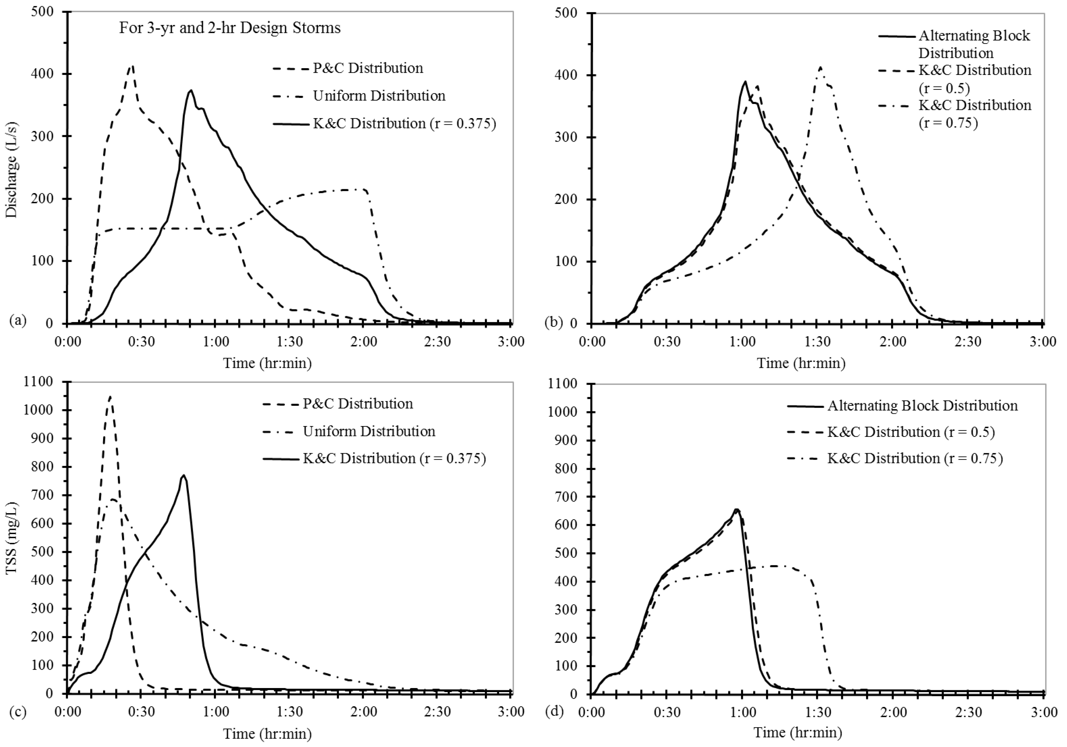
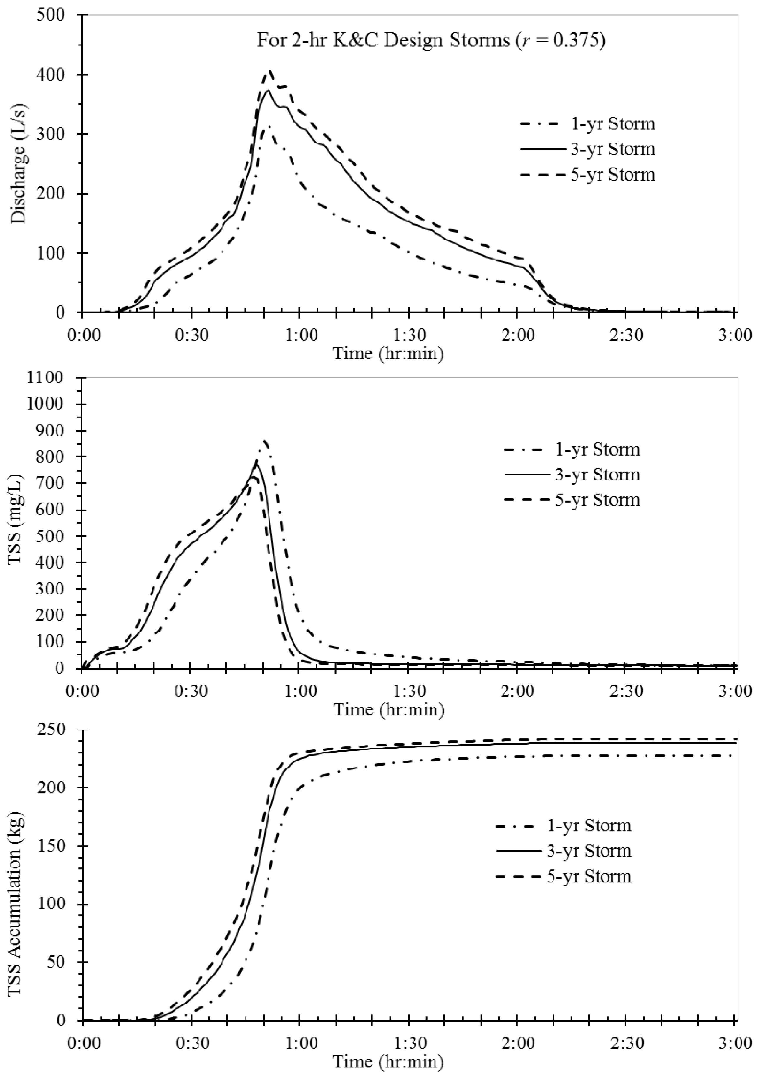
Pollutographs of TSS at the catchment outlet (Outfall in Figure 1) resulting from three different design rainfall distributions are shown in Figure 8, each under the assumption of five antecedent dry days. The initial buildup of TSS is 327.0 kg determined using Equation (1), and the three-year, 2-h storm delivers 24.2 kg of TSS from the wet deposition; therefore, total TSS available for washoff for each design rainfall in Figure 8 is 351.2 kg. For the same rainfall depth (63.4 mm), the peak concentration of TSS and the time of its appearance depend on the timing of peak rainfall (Figure 8), which is related to rainfall pattern (i.e., choice of hyetograph). The washoff load of TSS is a function of runoff and the amount of buildup remaining (Equation (2)). With the increase of discharge due to the increase (continuation) of rainfall over time, TSS concentration first increases with time and reaches a peak value, then decreases with time because the amount of previously accumulated pollutant that is remaining for washoff decreases with time. After the TSS concentration reaches its peak (Figure 8), it begins to decrease and eventually reaches a stable, low concentration (approximately 10 mg/L), which is the background rainfall TSS concentration.

Table 5. Summary of simulated Q_p and TSS characteristics for the three-year, 2-h design rainfall with different distributions (hyetographs).

Parameters/Rainfall Distribution	Uniform Distribution	P&C Distribution	K&C Distributions			Alternating Block
			r = 0.375	r = 0.5	r = 0.75
Depth (mm)	63.4	63.4	63.4	63.4	63.4	63.4
Peak Rainfall Intensity (mm/h)	31.7	165.9	156.5	127.9	148.1	161.3
Time of Peak Rainfall (min)	-	20	45	55	85	55
Peak Discharge (Qp, L/s)	214.9	415.9	374.1	382.6	413.1	390.1
Time of Qp (min)	120	26	51	66	91	61
Peak TSS (mg/L)	686.3	1047.8	772.9	651.9	455.4	656.5
Time of Peak TSS (min)	18	17	48	58	73	58
Outlet EMC (mg/L)	226.6	213.2	211.3	222.1	242.6	219.8
Outlet TSS Load (kg and % 1)	284.8 (91.8)	216.4 (67.7)	238.8 (75.2)	248.4 (78.1)	265.3 (83.3)	245.4 (77.2)
Surface Runoff TSS (kg and % 2)	310.2 (88.3)	319.4 (91.0)	317.6 (90.5)	318.0 (90.6)	318.5 (90.7)	318.0 (90.6)
TSS base time (min)	125	32	64	73	98	71
Flood volume (% 3)	14.3	37.7	27.9	29.0	31.2	29.1
TSS flood loss (% 4)	8.2	32.3	24.8	21.9	16.7	22.8

Notes: ¹ The percentage for this parameter is calculated from the ratio of the outlet TSS load to the surface runoff TSS because some TSS is lost due to surface flooding. This percentage is given as the number inside brackets; ² The percentage for this parameter is calculated from the ratio of the surface runoff TSS to the sum of TSS initial buildup and wet deposition because TSS loss includes the infiltration loss and any remaining accumulated TSS on the surface. This percentage is given as the number inside brackets; ³ This parameter is the ratio (expressed as a percentage) of total flood volume above the ground and the total surface runoff; ⁴ This measure is equal to 100% minus the outlet TSS load (in percentage, note 1), and is equal to TSS lost by surface flooding divided by the surface runoff TSS.

summarizes Q_p and TSS characteristics for the three-year, 2-h design rainfall distributed according to the different hyetographs. As a result of all but the uniform rainfall distributions, the TSS concentration reaches a peak value that precedes the peak discharge (Q_p) by 3 min to 18 min (Table 5) and decreases rapidly after the peak (Figure 8); this is the same behavior observed by Luo et al. [42]. The uniform rainfall distribution has no rainfall peak and results in a TSS peak concentration of 686.3 mg/L at 18 min (Table 5), followed by a gradual decrease of TSS concentration (Figure 8b). For the uniform rainfall distribution, the peak discharge of 214.9 L/s is lower than the peak discharges resulting from other rainfall distributions, and occurs at a much later time (120 min). 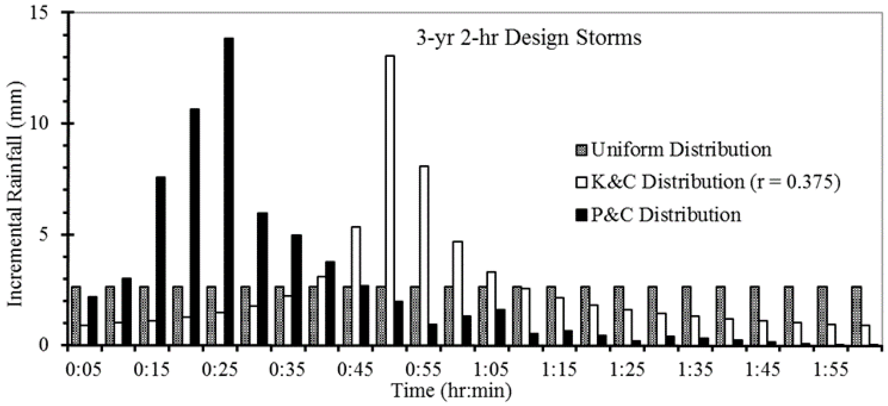Although all hyetographs produce the same rainfall depth, the simulated TSS peak concentration at the outfall is the highest for the P&C rainfall distribution because it results in the largest Q_p (415.9 L/s) at the earliest time (26 min), followed in descending order by the K&C distribution (with r = 0.375) and the uniform rainfall distribution. This result occurs because the P&C distribution has higher rainfall intensity in the first 25 min than the other two distributions (Figure 2), and because TSS concentration increases with an increase in initial rainfall intensity. The washoff ability of the P&C rainfall pattern is stronger than the K&C distribution and uniform rainfall distribution in the first 25 min. Once a large proportion of accumulated TSS has been washed off by runoff, TSS concentration decreases rapidly with time after the TSS concentration reaches its peak, a pattern that results from all design rainfall distributions except the uniform distribution (Figure 8). In contrast to other distributions, the uniform design rainfall results in smaller runoff discharges and no (or minimal) increase in runoff from 0:10 to 2:10; thus, TSS concentration gradually decreases with time after reaching its peak concentration.

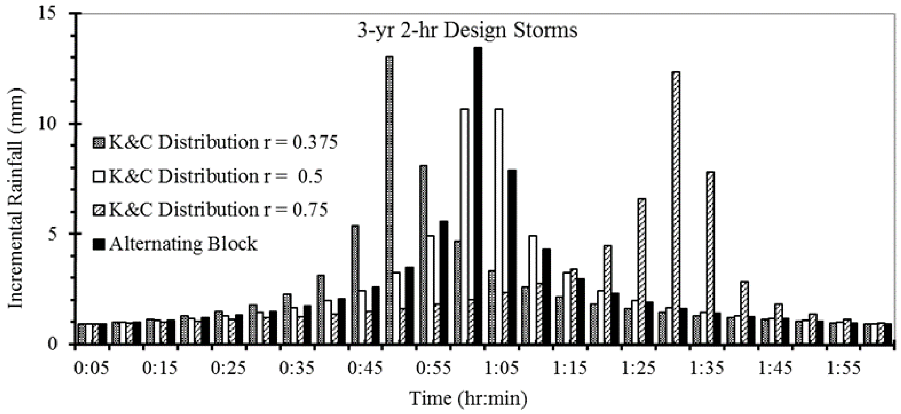
TSS concentrations resulting from the K&C rainfall distribution with the constant r equal to 0.5 were almost the same as those resulting from the alternating block rainfall distribution because these two rainfall distributions are very similar (Figure 3). Comparatively, however, the K&C distribution with the constant r equal to 0.75 has a later rainfall peak (148.1 mm/h at 85 min), which results in a gradual increase of TSS concentration that peaks at 455.4 mg/L (73 min). TSS concentrations resulting from the K&C distributions with the constant r equal to 0.375 and 0.5 are very similar, but when r was 0.375, the peak TSS concentration was 18% larger and occurred 10 min earlier than when r was 0.5 (Table 5). When the peak location constant r in the K&C distribution increases (0.375, 0.5, and 0.75), which ultimately results in a third-quartile storm, peak runoff discharge increases and peak TSS concentration decreases (Table 5). Nevertheless, both the outlet TSS load and event mean concentration (EMC) increase because the TSS flood loss decreases as r increases.

The EMC is commonly used to quantify the overall pollutant load of stormwater runoff and is defined as the event load divided by the event water volume [43]. The EMC in this study was calculated at the outfall of the catchment; therefore, it is equal to the outlet TSS load divided by the runoff volume integrated from the outlet hydrograph (Figure 8). As shown in Table 5, the EMC of TSS ranged from 211.3 mg/L to 242.6 mg/L (with both extremes resulting from K&C rainfall distributions). The P&C distribution, alternating block distribution and uniform distribution of the design rainfall results in outlet EMCs of 213.2 mg/L, 219.8 mg/L, and 226.6 mg/L, respectively. The differences in the EMCs from different rainfall distributions are much smaller than the differences in the TSS peaks that result from the distributions (Table 5).

The time bases of TSS pollutographs are given in Table 5 and range from 32 min (for the P&C distribution) to 125 min (for the uniform distribution), which were 26.7% to 104.2% of the rainfall duration. The TSS time bases for K&C distributions and alternating blocking distributions are similar (64–98 min). The TSS time base is larger when the rainfall distribution is more uniform and when the rainfall peak occurs later (e.g., a third-quartile storm represented by the K&C distribution with r = 0.75).

Table 5 also gives TSS load at the outlet (calculated using the flow and TSS distributions) and surface runoff TSS mass (kg) for each design rainfall distribution. The surface runoff TSS mass ranged from 310.2 kg to 319.4 kg, which was 88.3%–91.0% of the 351.2 kg total available TSS (Table 5). The resulting runoff from three-year, 2-h storms has adequate washoff capability to transport TSS; therefore, the surface runoff TSS loads for all hyetographs are similar (317.0 ± 3.4 kg) because the washoff is limited by available sediments from initial buildup and wet deposition, not by the transport capacity of the runoff. For the uniform, K&C (r = 0.375) and P&C rainfall distributions, the outlet TSS loads are calculated as 284.5 kg, 248.4 kg and 216.4 kg, respectively. The outlet TSS loads are 67.7%–91.8% of the surface runoff TSS, indicating that surface flooding deposits a certain amount of TSS above ground after flooding. The TSS “loss” due to flooding as a percentage of the total TSS transport by surface runoff range from 8.2% for the uniform rainfall distribution to 32.3% for the P&C distribution (last row of Table 5). The P&C rainfall distribution produces the earliest and highest peak discharge among all six rainfall distributions; therefore, the resulting outlet TSS load is the smallest (216.4 kg) because the surface flooding lasts approximately 58 min and has the largest overflow (flood) volume (614 m³). The uniform rainfall distribution results in the largest outlet TSS load (284.8 kg) because this distribution produces the smallest flooding volume (210 m³). However, the flooding duration (115 min) at junction J16 under the uniform rainfall distribution is longer than that from the P&C rainfall distribution because the runoff simulated from uniform rainfall has a slower and longer increase before reaching the peak than that from other distributions. The flood volume as a percentage of total surface runoff ranges from 14.3% for uniform rainfall to 37.7% for the P&C rainfall distribution (Table 5). As shown in Table 5, the total runoff volumes simulated for the six rainfall distributions are almost identical, with only 3.5% standard deviation (1568.7 ± 54.4 m³).

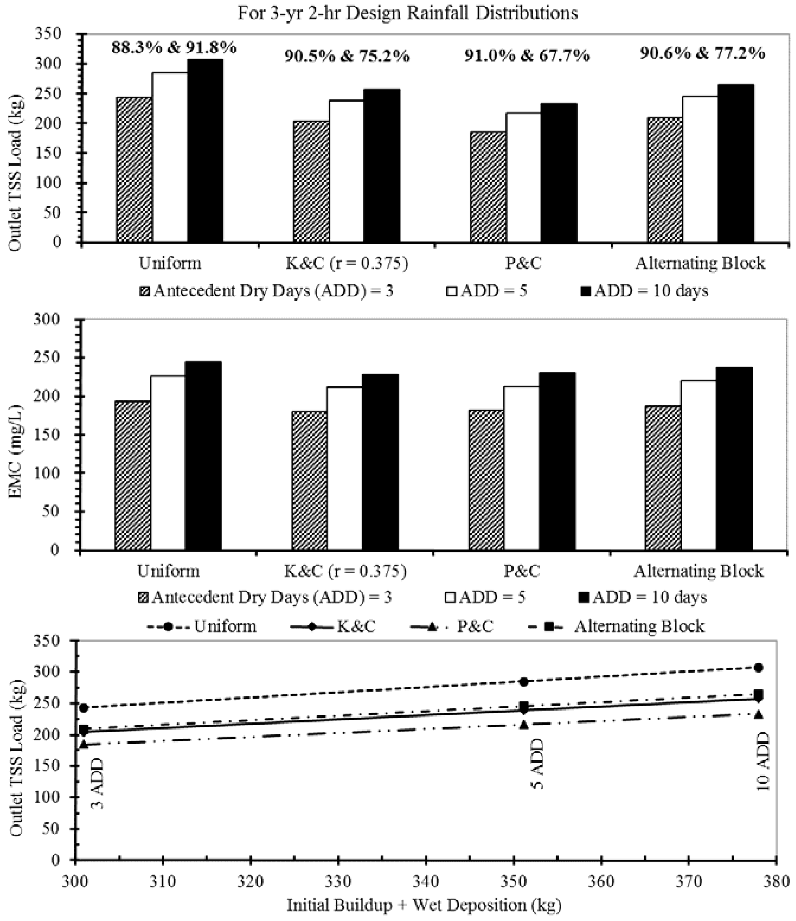
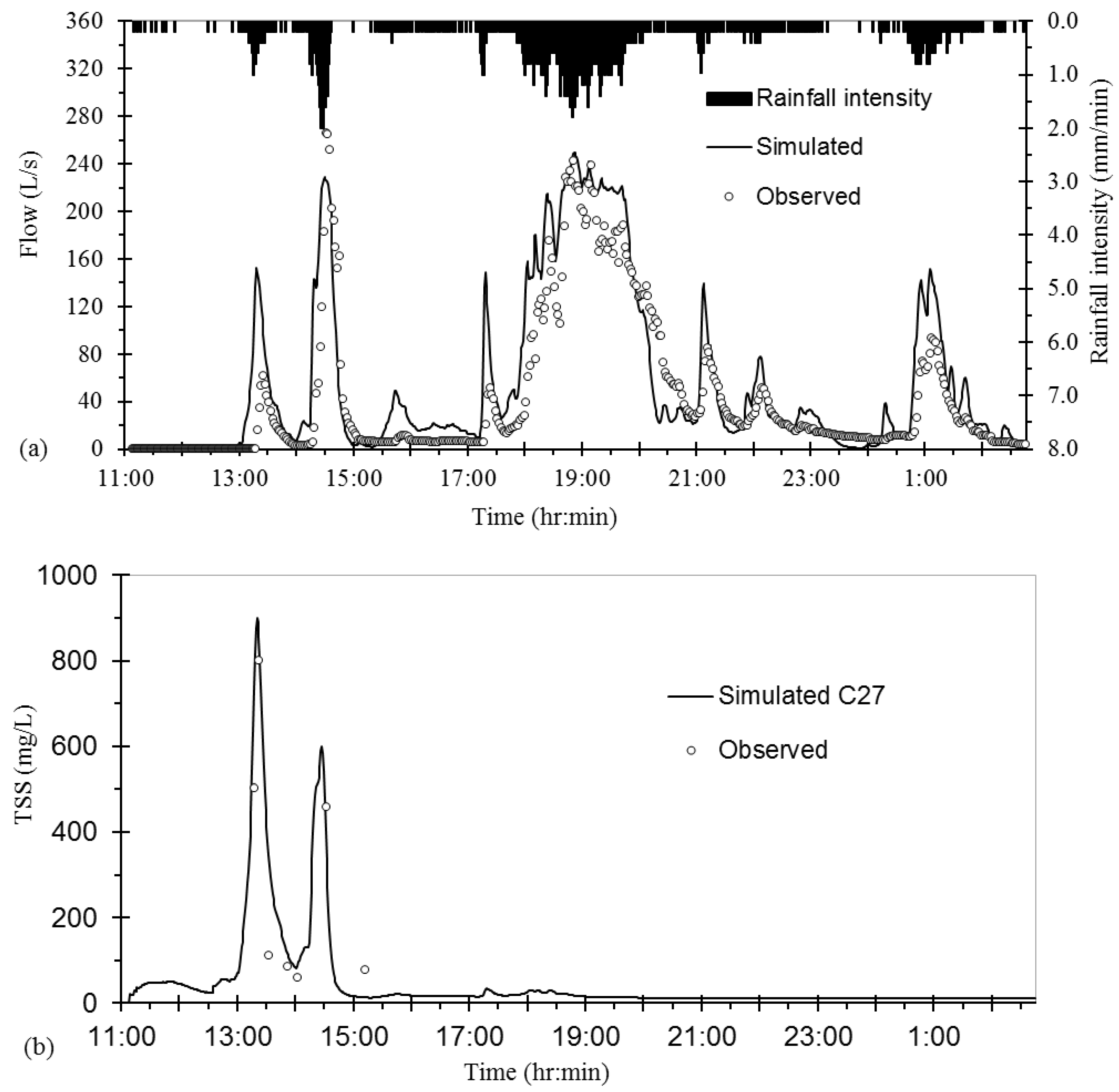
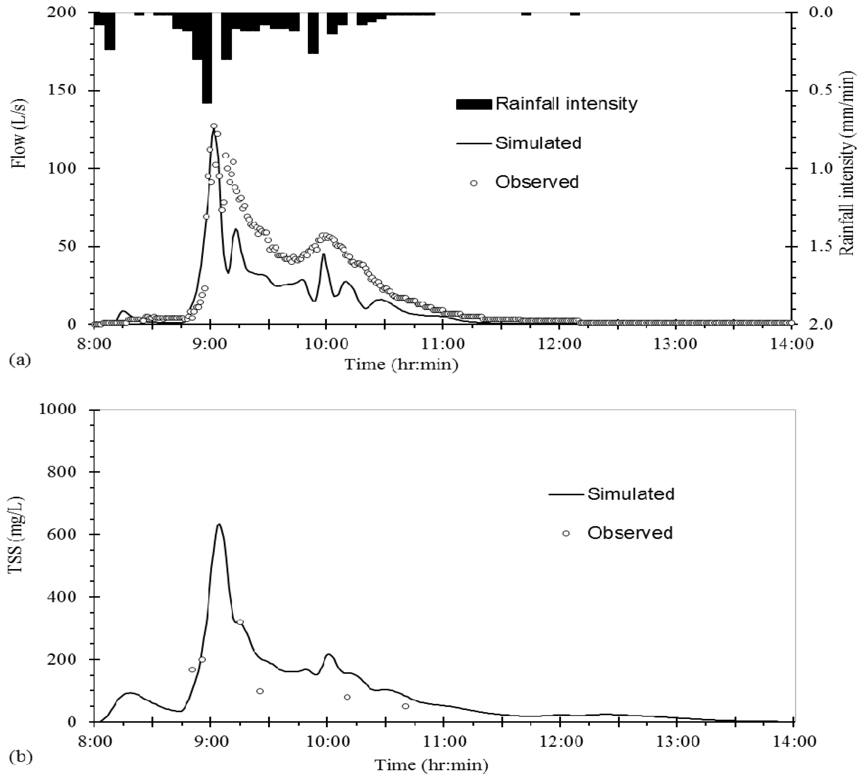
Results presented in Figure 8 and Table 5 were developed under the assumption of five antecedent dry days for all design storms in SWMM modeling. A sensitivity analysis was conducted using four design rainfall distributions to examine the effect of antecedent dry days (three days and 10 days); comparative results of the simulated outlet TSS loads and EMCs are given in Figure 9. As described in Section 3.1, the three-day and 10-day antecedent dry periods were happened for the 7 June 2013 model-validation event and the 21 July 2012 model-calibration event. The three and 10 dry days result in initial buildups of 276.8 kg and 353.8 kg TSS, respectively (Table 4). Because the volume of rainfall is the same for the four distributions, so is the mass of TSS in wet deposition (24.1 kg). Both the outlet TSS load and EMC have perfect linear correlations with the available sediment for transport (initial buildup plus wet deposition); this result can be explained using Equation (2) when discharges produced by the design rainfall are the same for three sensitivity model runs and assuming three antecedent dry days. In Figure 9, two percentages are given above the bars of the outlet TSS load for each design rainfall distribution. The first of these percentages is surface runoff TSS as a percentage of total available sediment for washoff or transport. The second percentage is the outlet TSS load as a percentage of surface runoff TSS. These two percentages for an assumption of five antecedent dry days are given in Table 4. Data shown in Figure 9 and Table 4 reveal that the two percentages are exactly the same for all three antecedent dry-day periods. The product of these two percentages gives the outlet TSS load as the percentage of total available sediment. Of the four rainfall distributions, the uniform design storm transported the highest percentage (81.1% = 88.3% × 91.8%) of total sediment because it yields the lowest TSS flood loss (8.2%), although runoff from the uniform rainfall has the lowest capability (88.3%) to wash off sediment. The P&C design storm transports the lowest percentage of total sediment (61.6%) because 32.3% of TSS load (i.e., 100%–67.7%) is trapped by surface flooding.

In summary, six design rainfall distributions (hyetographs) with the same return period (3 year) and duration (2-h) were examined using SWMM. The choice of hyetograph can significantly affect the shape and peak value of the resulting runoff hydrograph and thus the TSS pollutograph (Figure 8). The P&C rainfall distribution is a first-quartile storm (the most severe) and results in the highest peak discharge and TSS concentration at the outlet, but the lowest outlet TSS load because of the highest TSS loss due to flood deposition (32.3%). The uniform rainfall distribution results in the lowest peak discharge and the latest time to peak and the highest outlet TSS load, not because it has the highest washoff capability, but rather because it produces the smallest TSS loss due to flooding (8.2%). Fang et al. [44] also confirmed that the rainfall hyetograph is a major determinant of runoff pollution load. Huang and Nie [45] pointed out that the position of the rainfall peak in an event had a certain influence on urban NPS pollution. Others have shown that the removal of pollutants from pervious surfaces depends heavily on the rainfall hyetograph [46].

3.2.2. Influences of Rainfall Depth or Intensity

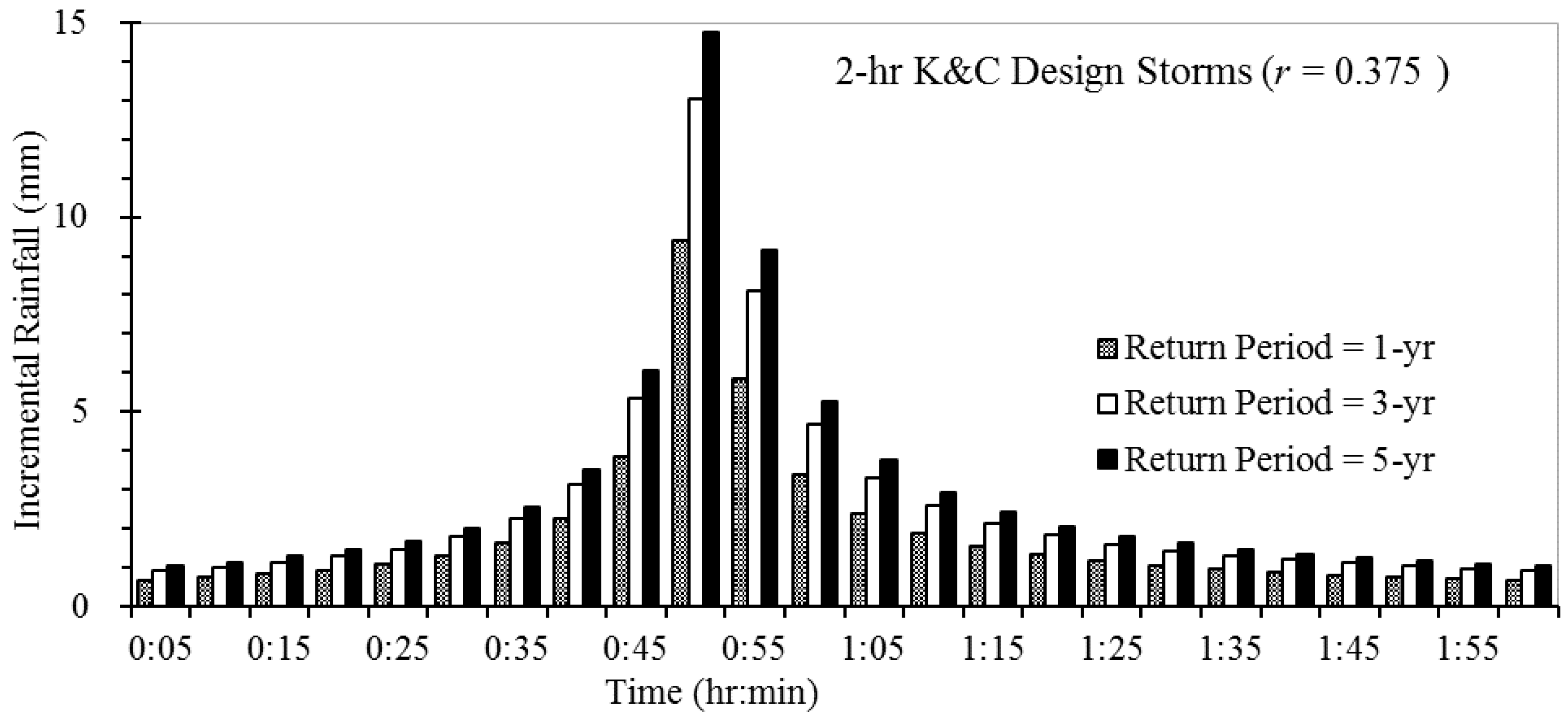
TSS resulted from different rainfall intensities are shown in Figure 10 using the 2-h K&C design storms (r = 0.375) having one-, three-, and five-year return periods. When the return period changes from one-year to five-year, total rainfall increases from 45.8 mm to 71.7 mm (Table 2); likewise, the 5-min peak rainfall intensity increases from 100.3 mm/h to 176.9 mm/h, but occurs at the same time (during 45–50 min, Table 1 and Table 4). The resulting peak discharges at the outlet are 341.2 L/s, 374.1 L/s, and 408.9 L/s with the same time to peak (51 min) for one-, three-, and five-year storms, respectively. For all SWMM simulations in this study, design rainfalls for 5-min intervals were used as model input, but outflow and TSS were predicted and reported at 1-min intervals. The results indicated that rainfall intensity has a certain impact on TSS concentration and total TSS load. However, the TSS accumulation processes are similar for rainfalls of different rainfall depths and intensities, and the TSS washed off by runoff mainly concentrates from 10 min to 55 min after the rainfall starts (Figure 10).

The TSS peak concentrations at the outlet for one-, three-, and five-year return periods are 859.4 mg/L, 772.9 mg/L, and 725.9 mg/L, respectively; and occur at 47 min to 50 min after the rainfall begins. Surface runoff volumes for one-, three-, and five-year design storms range from 942 m³ to 1582 m³ for the study catchment, but TSS due to initial build-up is constant (327.0 kg) owing to the use of a common antecedent dry period in all simulations. Tiefenthaler and Schiff [47] found that a greater runoff volume resulting from larger rainfall depth would dilute the concentration of a pollutant in runoff, reducing, for example, the TSS peak concentration.

The simulated total pollutant loads of TSS for the K&C design storms having one-, three-, and five-year return periods are 227.4 kg, 238.8 kg and 242.0 kg, respectively (

Table 6. Summary of simulated flow and TSS concentration characteristics for the 2-h K&C design storms (r = 0.375) with three different return periods.

Parameters/Return Periods	One-Year	Three-Year	Five-Year
Peak Rainfall Intensity (mm/h)	112.9	156.5	176.9
Time of Peak Rainfall (min)	45	45	45
Peak Discharge (Qp, L/s)	341.2	374.1	408.9
Time of Qp (min)	51	51	51
Peak TSS (mg/L)	859.4	772.9	725.9
Time of Peak TSS (min)	50	48	47
Outlet EMC (mg/L)	290.8	211.3	191.9
Outlet TSS Load (kg)	227.4	238.8	242.0
Surface Runoff Load (kg)	292.3	317.6	322.8
TSS base time (min)	104	64	60
Flood volume (%)	16.7	27.9	32.5
TSS flood loss (%)	22.2	24.8	25.0

). The results suggest that pollutant load at the outfall has a positive correlation (R² = 0.95) with rainfall depth and intensity, while the outlet EMC decreases from 290.8 mg/L for a one-year storm to 191.9 mg/L for a five-year storm (Table 6) because of the dilution effect. The one-year storm produces a larger TSS time base (104 min) because the TSS peak occurs slightly later and the smaller discharges makes TSS decrease slowly to the 30-mg/L cutoff limit when TSS < 100 mg/L (Figure 10). When the return period increases, the total pollution loads of TSS from the outlet also increases. Gnecco et al. [48] reported that there is a strong correlation between the EMC of TSS and the maximum rainfall intensity because rainfall intensity determines the surface pollutants washoff portion. Other studies have also shown that the amount of accumulated pollutant load washed off during rainfall event is dependent on rainfall and runoff characteristics [9]. As the return period increases, so too does rainfall intensity. Thus, in this study, as return period increases, the sediment in surface runoff gradually increases, and the resulting NPS pollution load increases. However, because the mass of contaminants available for wash off was limited, the increased rainfall intensity results in a decreasing trend in the amplitude of increases in the pollutant load.

The data analysis shows that, under the same rainfall hyetograph, simulated peak discharge and outlet TSS load are positively correlated (R² = 0.95) to the rainfall depth as a function of the return period, while peak TSS concentration and the outlet EMC have the negative correlation (R² = 0.95).

3.2.3. Influence of Rainfall Duration

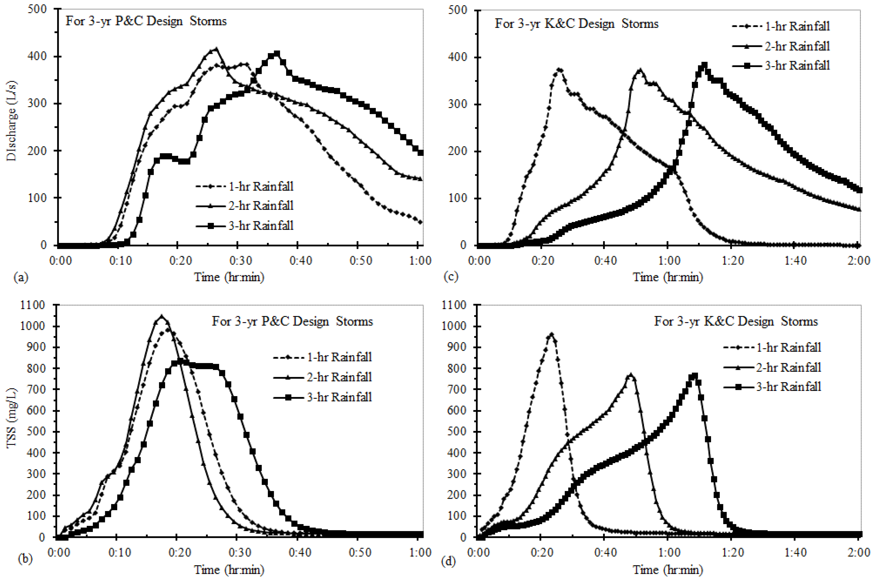
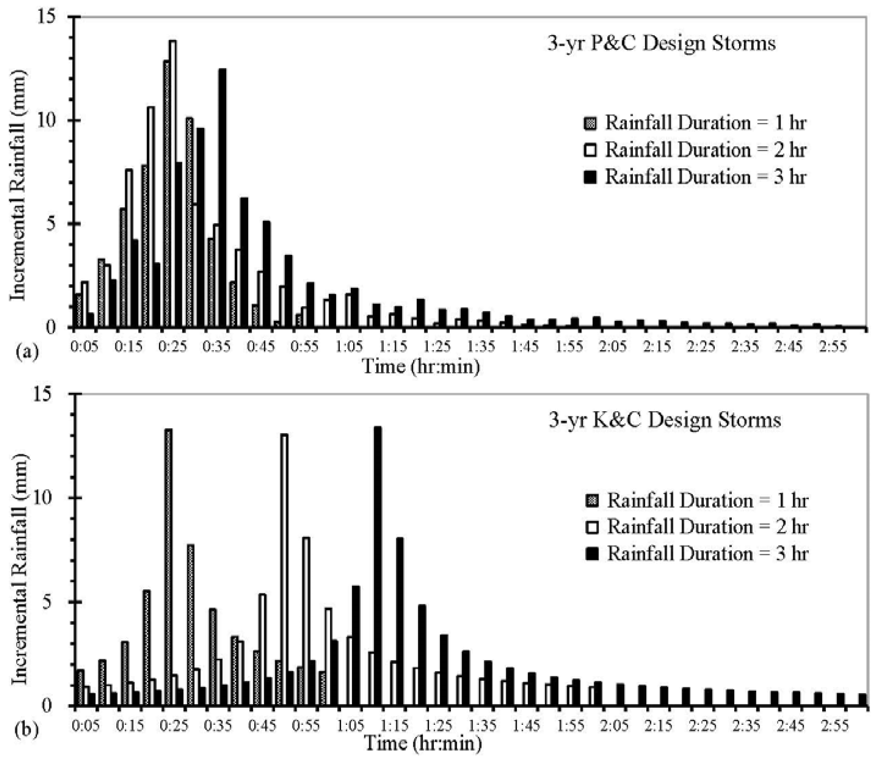
TSS resulted from different rainfall durations are shown in Figure 11 using three P&C design rainfall distributions, which were based on observed long-term heavy rainfall events in Beijing central districts [32], and three K&C rainfall distributions based on Beijing IDF curves. The P&C distributions have periods in which incremental rainfall during successive intervals can be either lower or higher than in the previous interval (Figure 5). The P&C distributions were different from the K&C distributions and the alternating block distribution (Figure 2, Figure 3 and Figure 4) in which the 5-min incremental rainfalls gradually increased to the peak rainfall and then gradually decreased. The results indicate that for the same total rainfall depth, the rainfall duration was a major factor of the urban NPS pollutant loads. Pollutographs in Figure 11 show that the TSS peak concentrations at the outlet for the 60-, 120- and 180-min rainfall durations were 983.7 mg/L, 1047.8 mg/L and 838.1 mg/L, respectively, for three-year P&C design rainfall distributions. Even though the average rainfall intensity of a short-duration rainfall event is greater than that of a long-duration event, incremental 5-min rainfall (or rainfall intensity) of the 2-h P&C distribution during the first 25 min is larger than for both the 1-h and 3-h P&C design storm rainfall distributions (Figure 5). Therefore, simulated discharge and TSS concentration at the outlet for the 2-h storm increase faster and reach higher peaks at earlier times than do these measures for 1-h and 3-h storm durations (Figure 11 and

Table 7. Summary of simulated TSS characteristics for the three-year P&C distribtuion of design rainfall with three different rainfall durations.

Parameters/Rainfall Durations	P&C Distributions			K&C Distributions
	1-h	2-h	3-h	1-h	2-h	3-h
Peak Rainfall Intensity (mm/h)	154.2	166.0	149.4	159.4	156.5	160.5
Time of Peak Rainfall (min)	20	20	30	20	45	65
Peak Discharge (Qp, L/S)	382.8	415.9	406.2	372.4	374.1	383.7
Time of Qp (min)	31	26	36	25	51	71
Peak TSS (mg/L)	983.7	1047.8	838.1	962.2	772.9	766.6
Time of Peak TSS (min)	18	17	20	23	48	68
Outlet EMC (mg/L)	308.6	213.2	198.5	273.8	211.3	189.6
Outlet TSS Load (kg)	221.9	216.4	234.5	217.7	238.8	240.8
Surface Runoff Load (kg)	312.7	319.4	321.8	311.0	317.6	320.7
TSS base time (min)	35	32	41	42	64	81
Flood volume (%)	40.5	37.7	34.5	32.3	27.9	27.3
TSS flood loss (%)	29.1	32.3	27.1	30.0	24.8	24.9

). For the 3-h P&C design storm distribution, lower rainfall at 15–20 min results in small decreases of discharge (17–21 min) prior to the occurrence of Q_p as well as in TSS concentration (838.1–807.8 mg/L at 21–26 min) after the TSS peak (at 21 min). The TSS time base for the 3-h storm is 41 min, which is only slightly larger than that for the 1- and 2-h storms (35 and 32 min, respectively; Table 7). For the period after the TSS time base, even though discharges at the outfall remain large (Figure 11), TSS concentrations are less than 30 mg/L because most of initial TSS buildup has already been washed off and transported through the outlet. Such is the case for the other scenarios shown in Figure 8 and Figure 10.

The resulting hydrographs and TSS pollutographs for 1-, 2-, and 3-h K&C distributions of rainfall from a three-year design storm has consistent patterns. Peak discharges and outlet TSS loads increase while peak TSS concentrations and the outlet EMCs decrease as the storm duration increases (Table 7). Likewise, the TSS time base increases from 42 to 81 min as design storm duration increases from 1 h to 3 h because these K&C distributions (Figure 5) have the same peak location constant (r = 0.375) and are similar second-quartile storms. For P&C distributions of three durations, the peak location with respect to total rainfall duration is not constant; therefore, simulated hydrographs and TSS pollutographs are not similar from one duration to another of P&C distributions.

Total pollution loads of TSS at the catchment outlet are 221.9 kg, 216.4 kg and 234.5 kg for the 60-, 120- and 180-min rainfall durations, respectively. The outlet TSS load from 3-h duration rainfall is slightly larger than loads from 1- and 2-h rainfall, perhaps because the pollutant load is related to rainfall flushing time of the pollutant washoff process. For any given rainfall volume, long-duration rainfall implies a long pollutant washing time, which in turn will wash away more pollutants than rainfall of a shorter duration.

As indicated by the above conclusions, there are close relationships between TSS concentration in runoff and rainfall characteristics (rainfall patterns, rainfall intensity and rainfall duration). Among these rainfall characteristics, rainfall intensity and duration are the two dominant factors that control the hydrologic response, an observation corroborates by others [49,50].

4. Summary and Conclusions

The influences of rainfall characteristics (rainfall hyetograph, rainfall intensity, and rainfall duration) on TSS were investigated using SWMM for a university campus in Beijing, China (a drainage area of 6.3 ha and approximately 76.5% impervious area). The SWMM model was developed, calibrated and validated using data from two observed rainfall events: 21 July 2012 (severe rainfall of 221.2 mm over 16 h, with a 20–50 year return period) and 7 June 2013 (16.6 mm rainfall). The E_NS coefficients exceeded 0.72 for discharge calibration and validation. These results were obtained when the “Allow Ponding” option in SWMM was not active, and indicated that the underground pipeline system in the study catchment was under-designed, causing surface flooding that did not flow back into the pipelines. Even with the limited observed TSS data available, E_NS values and absolute relative errors for TSS calibration and validation were in acceptable ranges. A series of sensitivity model runs under various design rainfall characteristics were conducted for the catchment where surface flooding was possible. Modeling results from SWMM showed the influences not only of rainfall characteristics but also of surface flooding on TSS concentration and load at the outlet. Results and conclusions from the case study is site specific and may not be generally applicable to all urban catchments but are representative of many catchments because urban surface flooding is a common occurrence in old-city districts that have aging infrastructure, especially under heavy rainfall conditions. The main conclusions of this study are summarized as follows:

(1) For any given rainfall amount (as defined by its return period and duration), the choice of rainfall distribution (hyetograph) can significantly affect the shape and peak value of the resulting runoff hydrograph and associated TSS pollutograph. The P&C rainfall distribution that defines a first-quartile storm (the most severe) results in the highest peak discharge and TSS concentration at the outlet, but the lowest outlet TSS load because of the highest TSS “loss” (i.e., local deposition) due to flooding (32.3%). In contrast, uniformly distributed rainfall results in the lowest peak discharge, the longest time to peak and the highest outlet load; however, the latter is not because uniformly distributed rainfall has the highest TSS washoff capability but rather because it produces the smallest TSS loss attributed to flood deposition (8.2%). The simulated TSS pollutograph from the K&C rainfall distribution with r equal to 0.5 was almost the same as that for the alternating block rainfall distribution because these two rainfall distributions are very similar. However, the K&C distribution with r equal to 0.75 has a later rainfall peak (resulting in a third-quartile storm) that causes a gradual increase of TSS and the lowest peak TSS concentration (455.4 mg/L at 73 min).

(2) In response to a given rainfall hyetograph (e.g., three-year, 2-h K&C distribution with r equal to 0.375), simulated peak discharge and outlet TSS load are positively correlated (R² = 0.95) to the rainfall depth as a function of the return period, while peak TSS concentration and the outlet EMC have the negative correlation (R² = 0.95). The flood volume and loss of TSS due to flood deposition increases from 16.7% to 32.5%, and from 22.2% to 25.0%, respectively, as the return period increases from 1 year to 5 year.

(3) The three-year P&C design storms with 1-, 2-, and 3-h durations were developed from long-term heavy rainfall events in Beijing and have dissimilar rainfall distributions (e.g., different locations of peak rainfall with respect to the duration). The 1-h and 3-h P&C distribution design storms result in lower peak discharge and TSS concentration, but higher outlet TSS load than 2-h storm does, because of lower TSS losses due to flood deposition (29.1% and 27.1%). The resulting hydrographs and TSS pollutographs for 1-, 2-, and 3-h K&C distribution design storms with a three-year return period have consistent patterns because the three K&C distributions have the same peak location constant (r = 0.375) for the second-quartile storms.

For NPS pollution control in the study catchment with under-designed underground pipe system, it is important to implement various source control strategies such as lower impact development, using bioretention facilities and green infrastructures to reduce stormwater NPS. At the same time, old undersized stormwater infrastructures should be remodeled and revitalized.

References

1. Li, C.; Hu, Y.; Liu, M. Research advance of urban non-point source pollution. Ecol. Mag. 2013, 32, 492–500. [Google Scholar]
2. Yin, C.Q. The Theory and Technology of Urban Non-Point Source Pollution; China Building Industry Press: Beijing, China, 2009. [Google Scholar]
3. Danz, M.E.; Corsi, S.R.; Graczyk, D.J.; Bannerman, R.T. Characterization of Suspended Solids and Total Phosphorus Loadings from Small Watersheds in Wisconsin; U.S. Geological Survey Scientific Investigations Report 2010-5039; U.S. Geological Survey: Reston, VA, USA, 2010.
4. U.S. EPA. Meeting the Environmental Challenge; EPA’s Review of Progress and New Directions in Environmental Protection; United States (U.S.) Environmental Protection Agency (EPA): Washington, DC, USA, 1990; p. 26.
5. Yoon, S.W.; Chung, S.W.; Oh, D.G.; Lee, J.W. Monitoring of non-point source pollutants load from a mixed forest land use. J. Environ. Sci. 2010, 22, 801–805. [Google Scholar] [CrossRef]
6. Wang, J.P.; Zhu, M.L. Nitrogen and Phosphorus Non-point Pollution for Urban Stormwater Runoff in Xiamen. J. Xiamen Univ. Technol. 2009, 17, 57–61. [Google Scholar]
7. Bilotta, G.S.; Brazier, R.E. Understanding the influence of suspended solids on water quality and aquatic biota. Water Res. 2008, 42, 2849–2861. [Google Scholar] [CrossRef] [PubMed]
8. Morquecho, R.; Pitt, R. Pollutant associations with particulates in stormwater. In Proceedings of the World Water and Environmental Resources Congress, Anchorage, AK, USA, 15–19 May 2005; pp. 4973–4999.
9. Vaze, J.; Chiew, F.H.S. Experimental study of pollutant accumulation on an urban road surface. Urban Water 2002, 4, 379–389. [Google Scholar] [CrossRef]
10. Mahbub, P.; Ayoko, G.A.; Goonetilleke, A.; Egodawatta, P. Analysis of the build-up of semi and non volatile organic compounds on urban roads. Water Res. 2011, 45, 2835–2844. [Google Scholar] [CrossRef] [PubMed] [Green Version]
11. Mahbub, P.; Ayoko, G.A.; Goonetilleke, A.; Egodawatta, P.; Kokot, S. Impacts of traffic and rainfall characteristics on heavy metals build-up and wash-off from urban roads. Environ. Sci. Technol. 2010, 44, 8904–8910. [Google Scholar] [CrossRef] [PubMed] [Green Version]
12. Rossi, L.; Krejci, V.; Rauch, W.; Kreikenbaum, S.; Fankhauser, R.; Gujer, W. Stochastic modeling of total suspended solids (TSS) in urban areas during rain events. Water Res. 2005, 39, 4188–4196. [Google Scholar] [CrossRef] [PubMed]
13. Herngren, L.; Goonetilleke, A.; Ayoko, G.A. Understanding heavy metal and suspended solids relationships in urban stormwater using simulated rainfall. J. Environ. Manag. 2005, 76, 149–158. [Google Scholar] [CrossRef] [PubMed] [Green Version]
14. Horowitz, A.J.; Elrick, K.A.; Smith, J.J. Monitoring urban impacts on suspended sediment, trace element, and nutrient fluxes within the City of Atlanta, Georgia, USA: Program design, methodological considerations, and initial results. Hydrol. Process. 2008, 22, 1473–1496. [Google Scholar] [CrossRef]
15. Borris, M.; Vikler, M.; Gustafsson, A.M.; Marsalek, J. Modelling the effects of changes in rainfall event characteristics on TSS loads in urban runoff. Hydrol. Process. 2014, 28, 1787–1796. [Google Scholar] [CrossRef]
16. Gorgoglione, A.; Gioia, A.; Iacobellis, V.; Piccinni, A.F.; Ranieri, E. A rationale for pollutograph evaluation in ungauged areas, using daily rainfall patterns: Case studies of the Apulian region in southern Italy. Appl. Environ. Soil Sci. 2016, 3, 1–16. [Google Scholar] [CrossRef]
17. Mahbub, P.; Goonetilleke, A.; Ayoko, G.A.; Egodawatta, P. Effects of climate change on the wash-off of volatile organic compounds from urban roads. Sci. Total Environ. 2011, 409, 3934–3942. [Google Scholar] [CrossRef] [PubMed] [Green Version]
18. Teledyne ISCO. 2150 Area Velocity Module. Available online: http://www.isco.com/products/products3.asp?PL=2021010 (accessed on 5 March 2016).
19. Teledyne ISCO. 6712 Full-Size Portable Sampler. Available online: http://www.isco.com/products/products3.asp?PL=201101010 (accessed on 23 January 2016).
20. Ministry of Environmental Protection of the People’s Republic of China. Water Quality-Determination of Suspended Substance-Gravimetric Method. Available online: http://kjs.mep.gov.cn/hjbhbz/bzwb/shjbh/sjcgfffbz/199007/t19900701_67165.htm (accessed on 25 November 2015).
21. Rossman, L.A. Storm Water Management Model User’s Manual Version 5.0, EPA/600/R-05/040; U.S. Environmental Protection Agency, National Risk Management Research Laboratory—Office of Research and Development: Cincinnati, OH, USA, 2010.
22. Danish Hydraulic Institute (DHI). MIKE URBAN Integrated Urban Water Modelling. Available online: https://www.mikepoweredbydhi.com/products/mike-urban (accessed on 8 March 2016).
23. Innovyze. InfoWorks ICM (Integrated Catchment Modeling). Available online: http://www.innovyze.com/products/infoworks_icm/ (accessed on 14 March 2016).
24. Liu, J. Regression of City: “7.21” Torrential Rains in Beijing. Available online: http://www.weather.com.cn/zt/kpzt/1696696.shtml (accessed on 20 August 2012).
25. Nash, J.E.; Sutcliffe, J.V. River flow forecasting through conceptual models part I—A discussion of principles. J. Hydrol. 1970, 10, 282–290. [Google Scholar] [CrossRef]
26. Bennis, S.; Crobeddu, E. New runoff simulation model for small urban catchments. J. Hydrol. Eng. 2007, 12, 540–544. [Google Scholar] [CrossRef]
27. Keifer, C.J.; Chu, H.H.; Keifer, C.J.; Chu, H.H. Synthetic storm pattern for drainage design. J. Hydraul. Div. 1957, 83, 1–25. [Google Scholar]
28. Qin, H.P.; Li, Z.X.; Fu, G. The effects of low impact development on urban flooding under different rainfall characteristics. J. Environ. Manag. 2013, 129, 577–585. [Google Scholar] [CrossRef] [PubMed]
29. Pilgrim, D.H.; Cordery, I. Rainfall temporal patterns for design floods. J. Hydraul. Div. 1975, 101, 81–95. [Google Scholar]
30. Hershfield, D.M. Extreme rainfall relationships. J. Hydraul. Div. 1962, 88, 73–92. [Google Scholar]
31. Huff, F.A. Time distribution of rainfall in heavy storms. Water Resour. Res. 1967, 3, 1007–1019. [Google Scholar] [CrossRef]
32. Pani, E.A.; Haragan, D.R. A Comparison of Texas and Illinois Temporal Rainfall Distributions: Fourth Conference on Hydrometeorolog; American Meteorological Society: Boston, MA, USA, 1981; pp. 76–80. [Google Scholar]
33. Asquith, W.H.; Bumgarner, J.R.; Fahlquist, L.S. A triangular model of dimensionless runoff producing rainfall hyetographs in Texas. J. Am. Water Resour. Assoc. 2003, 39, 911–921. [Google Scholar] [CrossRef]
34. Mou, J. Design Storm Pattern Analysis in the City of Beijing. Ph.D. Thesis, Lanzhou Jiaotong University, Lanzhou, China, 2011. [Google Scholar]
35. Chow, V.T.; Maidment, D.R.; Mays, L.W. Applied Hydrology; McGraw-Hill: New York, NY, USA, 1988. [Google Scholar]
36. Viessman, W.; Lewis, G.L. Introduction to Hydrology, 5th ed.; Pearson Education: Upper Saddle River, NJ, USA, 2003; Volume 612. [Google Scholar]
37. Robert, H. Analysis of the Hydrograph. Horton Hydrologic Laboratory Publication 101; Edward Bros: Ann Arbor, MI, USA, 1935; Volume 101. [Google Scholar]
38. Gironás, J.; Roesner, L.A.; Davis, J.; Rossman, L.A. Storm Water Management Model Applications Manual; National Risk Management Research Laboratory, Office of Research and Development, U.S. Environmental Protection Agency: Cincinnati, OH, USA, 2009.
39. Manning, M.J.; Sullivan, R.H.; Kipp, T.M. Nationwide Evaluation of Combined Sewer Overflows and Urban Stormwater Discharges—Volume III: Characterization of Discharges; EPA-600/2-77-064c (NTIS PB-272107); U.S. Environmental Protection Agency: Cincinnati, OH, USA, 1977.
40. Vanoni, V.A. Sedimentation Engineering; Manual and Report on Engineering Practice No. 54; American Society of Civil Engineers: Reston, VA, USA, 1975. [Google Scholar]
41. Li, H.; Yue, L.; Huang, Y. The study of the typical water quality parameters value determination method in SWMM. Water Supply Drain. 2011, 37, 159–162. [Google Scholar]
42. Luo, H.; Luo, L.; Huang, G.; Liu, P.; Li, J.; Hu, S.; Wang, F.; Xu, R.; Huang, X. Total pollution effect of urban surface runoff. J. Environ. Sci. 2009, 21, 1186–1193. [Google Scholar] [CrossRef]
43. Wanielista, M.P.; Yousef, Y.A. Stormwater Management; John Wiley & Sons, Inc.: Hoboken, NJ, USA, 1993; Volume 18, pp. 253–254. [Google Scholar]
44. Fang, N.F.; Shi, Z.H.; Li, L.; Guo, Z.L.; Liu, Q.J.; Ai, L. The effects of rainfall regimes and land use changes on runoff and soil loss in a small mountainous watershed. Catena 2012, 99, 1–8. [Google Scholar] [CrossRef]
45. Huang, G.R.; Nie, T. Characteristics and load of non-point source pollution of urban rainfall runoff in Guangzhou, China. J. South China Univ. Technol. 2012, 40, 142–148. [Google Scholar]
46. Zhao, J.W.; Shan, B.Q.; Yin, C.Q. Pollutant loads of surface runoff in Wuhan City Zoo, an urban tourist area. J. Environ. Sci. 2007, 19, 464–468. [Google Scholar] [CrossRef]
47. Tiefenthaler, L.L.; Schiff, K.C. Effects of rainfall intensity and duration on first flush of stormwater pollutants. In Southern California Coastal Water Research Project Annual Report; Southern California Coastal Water Research Project: Westminster, CA, USA, 2001; pp. 209–215. [Google Scholar]
48. Gnecco, I.; Berretta, C.; Lanza, L.G.; Barbera, P.L. Storm water pollution in the urban environment of Genoa, Italy. Atmos. Res. 2005, 77, 60–73. [Google Scholar] [CrossRef]
49. Ran, Q.H.; Su, D.Y.; Li, P.; He, Z.G. Experimental study of the impact of rainfall characteristics on runoff generation and soil erosion. J. Hydrol. 2012, 424–425, 99–111. [Google Scholar] [CrossRef]
50. Rodríguez-Blanco, M.L.; Taboada-Castro, M.M.; Taboada-Castro, M.T. Rainfall–runoff response and event-based runoff coefficients in a humid area (northwest Spain). Hydrol. Sci. J. 2012, 57, 1–15. [Google Scholar] [CrossRef]
Figure 1. The stormwater management model (SWMM) model configuration for the study area including 30 sub-catchments (S1–S30), 30 junctions (J1–J30), underground pipes (thick solid lines with arrows for flow directions), monitoring point, and weather station.
Water 08 00278 g001
Figure 2. Three rainfall distributions used in SWMM model simulations for three-year, 2-h Beijing design storms.
Water 08 00278 g002
Figure 3. Beijing Keifer and Chu (K&C) design rainfall distributions for r = 0.375, 0.5, and 0.75, and alternating block rainfall distribution used in SWMM model simulations for three-year, 2-h design rainfall.
Water 08 00278 g003
Figure 4. Two-hour Beijing K&C design rainfall distributions for one-, three-, and five-year return periods.
Water 08 00278 g004
Figure 5. Three-year Beijing design rainfall distributions using the P&C method (a) and the K&C method (b) for three rainfall durations.
Water 08 00278 g005
Figure 6. Simulated and observed flow (L/s) (a) and TSS concentration (mg/L) (b) for the SWMM model calibration on 21 July 2012 including observed rainfall hyetograph.
Water 08 00278 g006
Figure 7. Simulated and observed flow (L/s) (a) and TSS concentration (mg/L) (b) for the SWMM model validation on 7 June 2013 including observed rainfall hyetograph.
Water 08 00278 g007
Figure 8. Simulated discharge (L/s) (a,b) and TSS concentration (mg/L) (c,d) at the catchment outlet for different three-year, 2-h design rainfall distributions.
Water 08 00278 g008
Figure 9. Simulated outlet TSS load (kg) and event mean concentration (EMC) of outlet TSS (mg/L) under three different antecedent dry-day periods for four three-year, 2-h design rainfall distributions, including the correlation between the outlet TSS load and available sediment (initial build-up plus wet deposition).
Water 08 00278 g009
Figure 10. Simulated discharges (L/s), TSS concentration (mg/L), and accumulative TSS export (kg) at the catchment outlet for one-, three- and five-year return periods of 2-h duration K&C design rainfall distributions.
Water 08 00278 g010
Figure 11. Simulated discharge (L/S) and TSS concentration (mg/L) at the catchment outlet under three-year design rainfall distributed using the P&C method (a,b) and K&C method (c,d) for three rainfall durations (1, 2 and 3 h).
Water 08 00278 g011