Article

Variability of Bed Drag on Cohesive Beds under Wave Action

United States Geological Survey, 384 Woods Hole Road, Woods Hole, MA 02543, USA
Water 2016, 8(4), 131; https://doi.org/10.3390/w8040131
Submission received: 1 February 2016 / Revised: 25 March 2016 / Accepted: 29 March 2016 / Published: 1 April 2016

Abstract

:
Drag force at the bed acting on water flow is a major control on water circulation and sediment transport. Bed drag has been thoroughly studied in sandy waters, but less so in muddy coastal waters. The variation of bed drag on a muddy shelf is investigated here using field observations of currents, waves, and sediment concentration collected during moderate wind and wave events. To estimate bottom shear stress and the bed drag coefficient, an indirect empirical method of logarithmic fitting to current velocity profiles (log-law), a bottom boundary layer model for combined wave-current flow, and a direct method that uses turbulent fluctuations of velocity are used. The overestimation by the log-law is significantly reduced by taking turbulence suppression due to sediment-induced stratification into account. The best agreement between the model and the direct estimates is obtained by using a hydraulic roughness of 10 - 4 m in the model. Direct estimate of bed drag on the muddy bed is found to have a decreasing trend with increasing current speed, and is estimated to be around 0.0025 in conditions where wave-induced flow is relatively weak. Bed drag shows an increase (up to fourfold) with increasing wave energy. These findings can be used to test the bed drag parameterizations in hydrodynamic and sediment transport models and the skills of these models in predicting flows in muddy environments.

1. Introduction

Bottom shear stress ( τ b ) affects turbulent mixing in water, flow momentum, vertical structure of flow in the water column, and, therefore, water circulation. This makes bed drag critical for not only sediment mobility and transport but also ecological, biological, and chemical processes in water [1,2]. The turbulent part of the direct estimate of τ b is - ρ u w ¯ (turbulent vertical transport of horizontal momentum, i.e., Reynolds stress) where ρ is the density of water, the overbar indicates Reynolds averaging, u is the horizontal velocity, w is the vertical velocity, and prime denotes turbulent fluctuations (e.g., [3]). Bottom shear stress is parametrized as τ b = ρ u * 2 where u * is the bottom friction velocity. Through quadratic drag relation τ b = ρ C d U c u r 2 , where U c u r refers to the horizontal mean current velocity, bed drag coefficient is estimated as C d = u * / U c u r 2 . Estimates of bed drag based on field observations are essential to understanding natural conditions. These field estimates of bed drag can be also used to calibrate hydrodynamic and sediment transport models and test the bed drag parametrizations implemented in these models.
A common empirical method to get indirect estimates of bed drag is to assume that the vertical structure of horizontal current velocity follows the logarithmic law of the wall [4]. This log-law is practical as it uses the mean current velocity profiles instead of the covariance of turbulent velocity fluctuations. However, the log-law is difficult to apply in weak flow conditions and it does not account for stratification effects on flow. Near-bed stratification due to sediment resuspension can reduce the bottom drag [5,6,7,8]. On the other hand, as shown by field measurements [9] and model predictions [10], surface wave-induced turbulence within the relatively thin wave boundary layer near the bed nonlinearly interacts with steady current flow and enhances bottom friction, which affects the vertical structure of flow throughout the water column. Numerical bottom boundary layer models are useful for investigating these combined wave-current flow and sediment processes [11], but these models usually include calibration parameters that introduce uncertainties to bottom stress estimates, and they can also be computationally expensive. Simplified theoretical models of combined wave-current flow in the bottom boundary layer [12] are also based on more restrictive assumptions. Therefore, direct estimates of bottom stress which use measurements of turbulent fluctuations of velocity instead of relying on the assumptions of numerical or empirical models are critical. In field settings where waves are energetic, wave-induced velocity fluctuations introduce bias to direct estimates of bottom stress. Relatively simple methods to reduce this wave bias, such as ensemble averaging (in the time domain) and high-pass filtering (in the frequency domain) are not easily applicable in field conditions where dominant wave frequency varies. One common method to obtain a direct estimate of bottom stress in wave-energetic field environments is to apply a linear filter between synchronized pressure and velocity measurements and identify velocity fluctuations coherent with pressure as wave oscillations [13]. However, this approach does not account for wave directionality or nonlinear waves. In order to reduce wave bias in direct estimates of stress, and also to account for nonlinear waves and wave directionality, a method that uses two synchronized velocity sensors estimates the stress as the covariance of the horizontal velocity difference between the two sensors and the vertical velocity difference between the two sensors [14].
Although there have been several studies on bed drag in sandy environments (e.g., [6,15,16,17,18,19,20]), bed drag in muddy environments and its variation with wave energy have remained relatively unexplored. In this study, the variation of bed drag under combined wave and current flow on a shallow, muddy shelf is investigated. Bottom stresses are estimated using (i) the indirect empirical log-law method; (ii) a bottom boundary layer model for combined wave-current flow; and (iii) the direct dual-sensor method that uses turbulent velocity fluctuations. The inter-comparison among these different methods is done. The variation of bottom stress and bed drag as a function of wave and current flow and stratification conditions is evaluated.

2. Materials and Methods
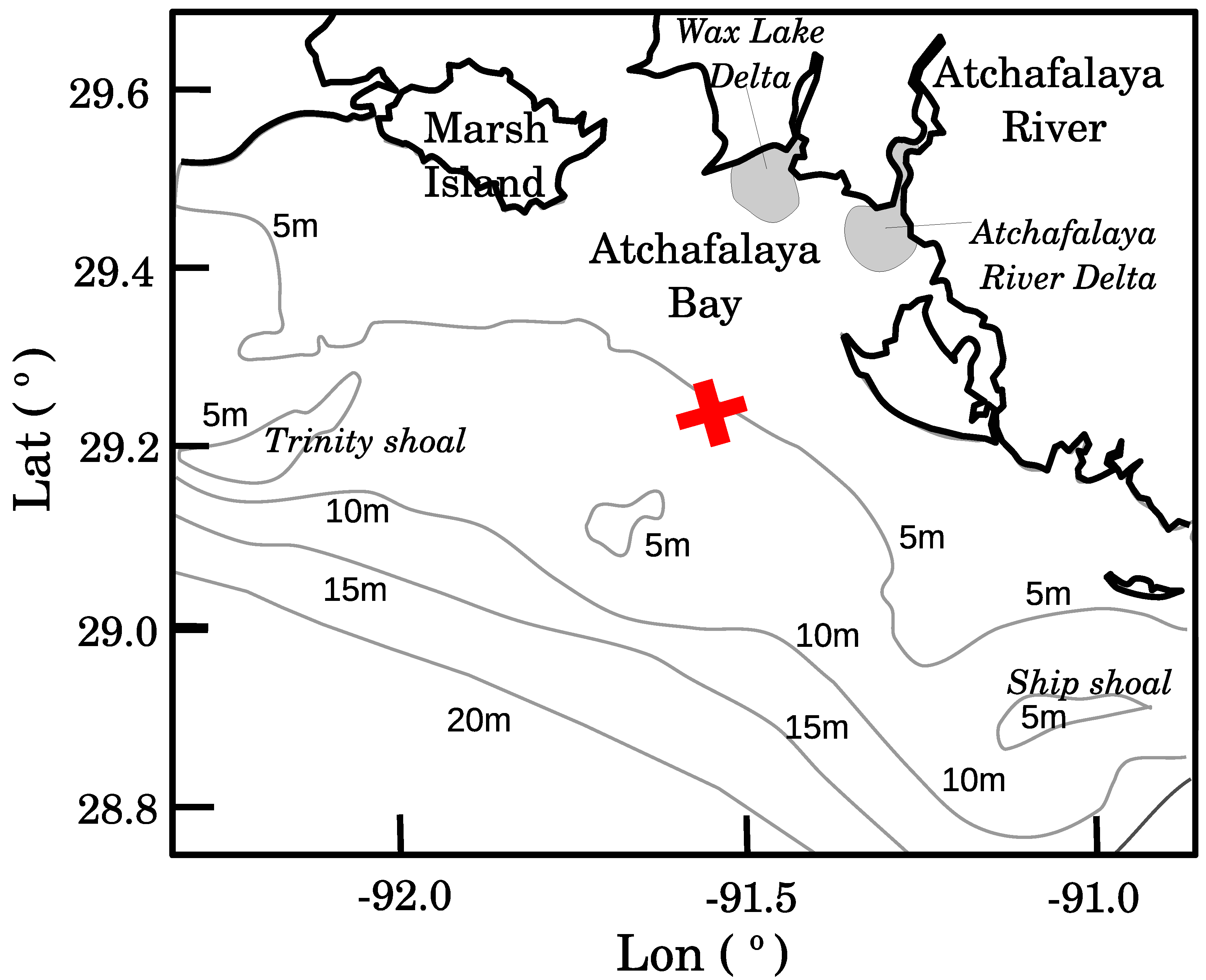
2.1. Study Site

The study site is the muddy Atchafalaya Shelf in the northern Gulf of Mexico, USA (Figure 1). The Atchafalaya Shelf was selected due to its very mild slope (~0.1%) and large mud input to the shelf by the Atchafalaya River. This high discharge of mud is noted to both cause accretion over the shelf and experience net westward transport due to prevailing winds. The two-week-long data set was collected at 5 m water depth between 26 March and 8 April 2008, during spring when waves and currents are energetic in the area due to periodic storms. Flows associated with these winter and early spring storms control the shelf circulation and sediment transport over the shelf. Tides are controlled mainly by a diurnal signal with average water level changes of about 0.6 m amplitude. Bottom sediment, dominated by cohesive sediments with relatively small fine sand content, is characterized with a median primary particle diameter of D 50 = 5 μm, which is classified as very fine silt. For a more detailed description of the atmospheric and oceanic conditions and the sedimentology of the field site, the reader is referred to related references [21,22].

2.2. Field Experiment

The configuration of the instruments on the platform is shown in Figure 2. Two Acoustic Doppler Velocimeters (ADV, SonTek, San Diego, CA, USA) collected synchronized measurements of pressure and three components of velocity at 10 Hz. Both of the ADVs sampled for 10 min every hour. One ADV was upward-pointing with its velocity sampling volume at 145 cm above bed and pressure sensor at 87 cm above bed; the other ADV was downward-pointing with its velocity sampling volume at 17 cm above bed and pressure sensor at 75 cm above bed. The vertical separation between the two velocity sensors ( r s , 128 cm) and the vertical distance of the bottom sensor above the bed ( z b , 17 cm) were set to satisfy the r s / z b > 5 requirement for achieving low cross-sensor correlation of turbulence-induced velocities [23]. Power-spectra were obtained based on these ADV measurements, with a frequency resolution of 0.02 Hz and 22 degrees of freedom, and used for determining bulk wave parameters such as significant wave height, bottom orbital velocity, etc.
A downward-pointing Pulse Coherent Acoustic Doppler Profiler (PC-ADP, Sontek/YSI, San Diego, CA, USA) collected high-resolution observations of pressure and vertical structure of near-bed flows and acoustic backscatter. These near-bed measurements were collected at 2 Hz in 27 bins of 3.2 cm, with a 15 cm blanking distance between the signal transmissing head and the first measurement bin, where no data is available, for the system to recover from acoustic pulse transmission. In synchronization with the PC-ADP, two Optical Backscatter Sensors (OBS-3, D&A Instruments, Port Townsend, WA, USA) measured turbidity. Both OBS-3 sensors were calibrated using field samples of sediment and water, collected at the study site, to estimate suspended sediment concentration. The OBS-3s were mounted at 16 and 42 cm above bed. In addition to these water column measurements, wind velocities above the sea surface were measured using an Onset HOBO station.

2.3. Methods

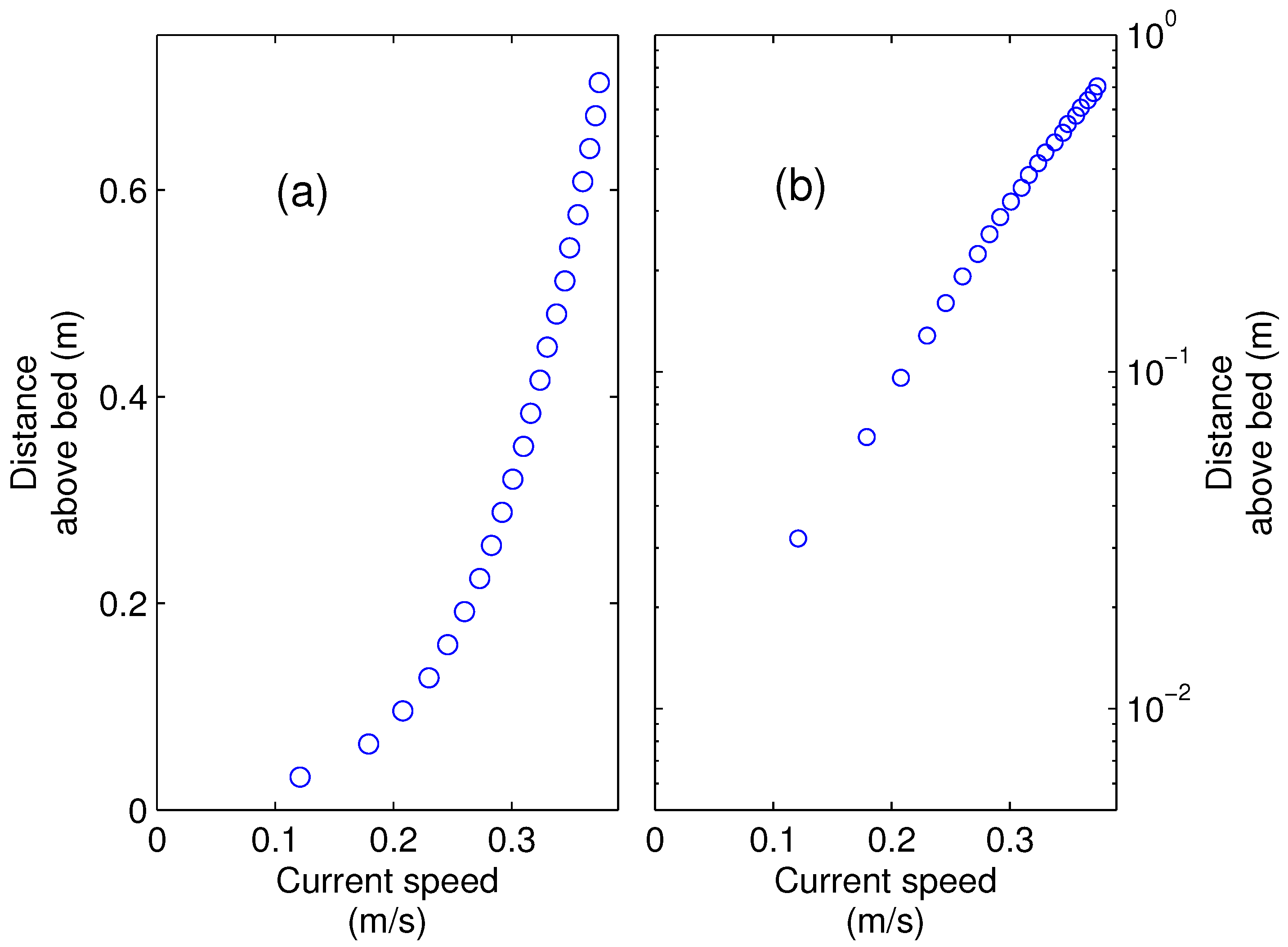
2.3.1. Logarithmic Law of the Wall

The logarithmic law of the wall (log-law) in an unstratified turbulent boundary layer states:
u ( z ) ¯ u * = 1 κ l n z z o
where κ = 0.41 is von Karman’s constant, z is the distance above bed, and z o describes a finite elevation above the bed where the velocity is assumed to be zero. Commonly, z o is defined by relating it to hydraulic roughness as k s = 30 z o [24]. As surface waves enhance the bed drag experienced by currents due to near-bed turbulence within the wave boundary layer [9,10], u * is estimated in this study by reconstructing logarithmic profiles (Equation (1)) in a least-squares sense based on the PC-ADP current velocity profiles ( u ( z ) ¯ ) outside the wave boundary layer of a few cm [25]. The logarithmic fitting is done iteratively; after excluding the first two bins above the bed, it starts by fitting the velocity measurements at the first three bins above those two bins. The first profile is accepted if r 2 > 0 . 9 where r is the correlation coefficient. The bins above the first three bins are added into the logarithmic fit as long as the resulting r 2 increases. Further details on this procedure can be found in the related references [22,26]. Log-law estimates of bottom stress ( τ b = ρ u * 2 ) were obtained from logarithmic layers spanning the entire PC-ADP profiling range for 86% of the experiment duration with an average r 2 = 0.98.

2.3.2. Bottom Boundary Layer Model

A bottom boundary layer model for combined wave-current flow [12] is used here. In this model, turbulence closure is achieved with a two-layer eddy viscosity formulation, where the eddy viscosity is time-invariant and scales with (i) bottom friction velocity due to combined wave-current flow within the wave boundary layer; and (ii) bottom friction velocity due to current flow outside the wave boundary layer. The bottom boundary layer model inputs are the current speed at a given height, bottom wave orbital velocity and excursion amplitude, the angle between current direction and wave direction, and hydraulic roughness, k s . The model procedure to estimate bottom stress τ b is iterative. In the first iteration, current-induced forcing is taken as zero; a wave friction factor is estimated; and a first approximation of bed stress is obtained. The relative importance of waves is updated in the model using this first approximation of stress, and this iterative procedure is repeated until a convergence within 1% is obtained, which is generally achieved within a few iterations. Further details on the physics and operation of the model can be found in the related reference [12]. Here, bottom stress ( τ b ) estimates from the model are obtained for k s = 10 - 5 m, 10 - 4 m, 10 - 3 m, the first of which corresponds to 2 D 50 (Section 2.1), i.e., the roughness due to only the primary sediment particle on the bed [24,27].

2.3.3. Dual-Sensor Method

The dual-sensor approach is based on the assumption that wave- and turbulence-induced velocities are uncorrelated; it also requires the correlation between the two sensors to be low for turbulence-induced velocities and high for wave-induced velocities. The initially proposed method [14] was advanced, to further reduce wave bias, by differencing after mapping the velocities at one of the sensors based on the velocities at the other sensor using linear filtration [28]. Near-bed Reynolds stress is directly estimated as the negative product of the water density and the integral of the real part of the cross-spectrum (i.e., co-spectrum, [29]) of the horizontal velocity difference and the vertical velocity difference between the two sensors:
τ b = - ρ u 1 w 1 ¯ - ρ 0 C o Δ u , Δ w ( f ) d f
Subscripts denote the number of velocity sensor (ADV), C o denotes co-spectrum, f is the frequency, Δ u = u 1 - u 21 and Δ w = w 1 - w 21 , such that subscript 21 denotes the velocity measured at ADV-2 and mapped to ADV-1 using least squares linear adaptive filtering [30]. Mapped velocities are the velocity fluctuations due to wave motion, correlated at the two sensors. Cross-spectra are obtained with a frequency resolution of 0.02 Hz and 22 degrees of freedom, like the spectra used for obtaining bulk wave parameters. For about half of the experiment duration, direct estimates of near-bed stress are obtained [31].
A full description of near-bed stresses would also include the viscous shear stress, i.e., τ ν = ρ ν ( d u / d z ) , where ν is the kinematic viscosity of water. Therefore, τ ν is calculated within the profiling range of the current profiler (which does not resolve the viscous sublayer) and is found to be O (0.001 Pa), much smaller than the near-bed Reynolds stress estimates, and is not shown here. It also needs to be mentioned that while the Reynolds stresses are estimated here in a more direct manner (by taking the actual turbulent fluctuations of velocity into account) compared to the two other methods, there is still the major assumption, for using this Reynolds stress as an estimate of bed stress, that the measurement elevation (17 cm above bed in the case herein) is within the constant stress region.

2.3.4. Wind Stress

In addition to the near-bed stress estimates based on the three methods described above, wind stress at the sea surface is also calculated. For this, the air–sea drag coefficient is calculated [32]. The formulation used herein is based on the results of an eddy correlation method that used open ocean momentum flux measurements. As a function of wind speed, the method gives the air-sea drag coefficient, which is used for estimating wind stress at the sea surface.

3. Results

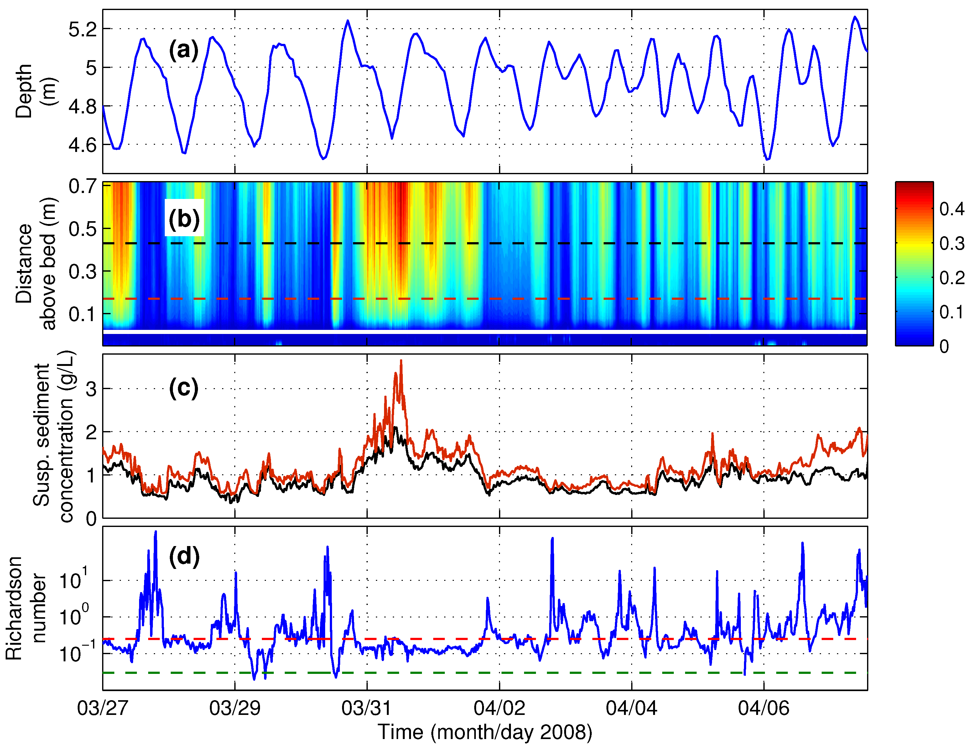
3.1. Field Observations

Figure 3 and Figure 4 summarize the conditions observed during the two-week-long experiment. Part of the ADV observations were presented before [31], so they were briefly discussed here. Winds were northward for most of the experiment (Figure 3a), with an average speed of 5.6 m/s. The sudden shift in wind direction to southward on 5 April (Figure 3a) is a characteristic of the typical atmospheric cold fronts that pass over the Atchafalaya Shelf in early spring. The strongest wind event observed was of moderate energy, with speeds reaching 12 m/s on 31 March (Figure 3a). Short wave energy at frequencies greater than 0.2 Hz (Figure 3b) and significant wave height in this band, with a maximum of 1 m (Figure 3d), are correlated with the wind energy (Figure 3a). The swell band (longer waves defined as frequencies less than 0.2 Hz) mostly had significant wave heights less than 0.25 m but had a spectral peak (Figure 3b) with significant wave heights exceeding 0.5 m on 5 April (Figure 3d), coinciding with the shift in wind direction (Figure 3a). Waves were mostly northward during the experiment (Figure 3c), but they also switched direction on 5 April, similar to the winds. Wave orbital velocities at the bed ( U o r b ) during the swell peak at 5 April were near 0.6 m/s (Figure 3e) and greater than those observed during the strongest wind event. Mean water level changes, dominated by a diurnal tidal signal, were about 0.6 m on average and reached 0.7 m during the strongest wind event (Figure 4a). Near-bed currents show the variability associated with the diurnal tides. The average current speed at 70 cm above bed was 0.19 m/s; winds exceeding 10 m/s on 31 March triggered current speeds of about 0.5 m/s (Figure 4b). The vertical structure of currents on 31 March, 10:00 is shown in Figure 5, in both linear (Figure 5a) and logarithmic (Figure 5b) scales in order to demonstrate the logarithmic layers formed near bed. Near-bed suspended sediment concentrations varied between 0.5 and 4 g/L and reached a maximum on 31 March (Figure 4c), coinciding with the peak of the winds, currents, and wave energy.

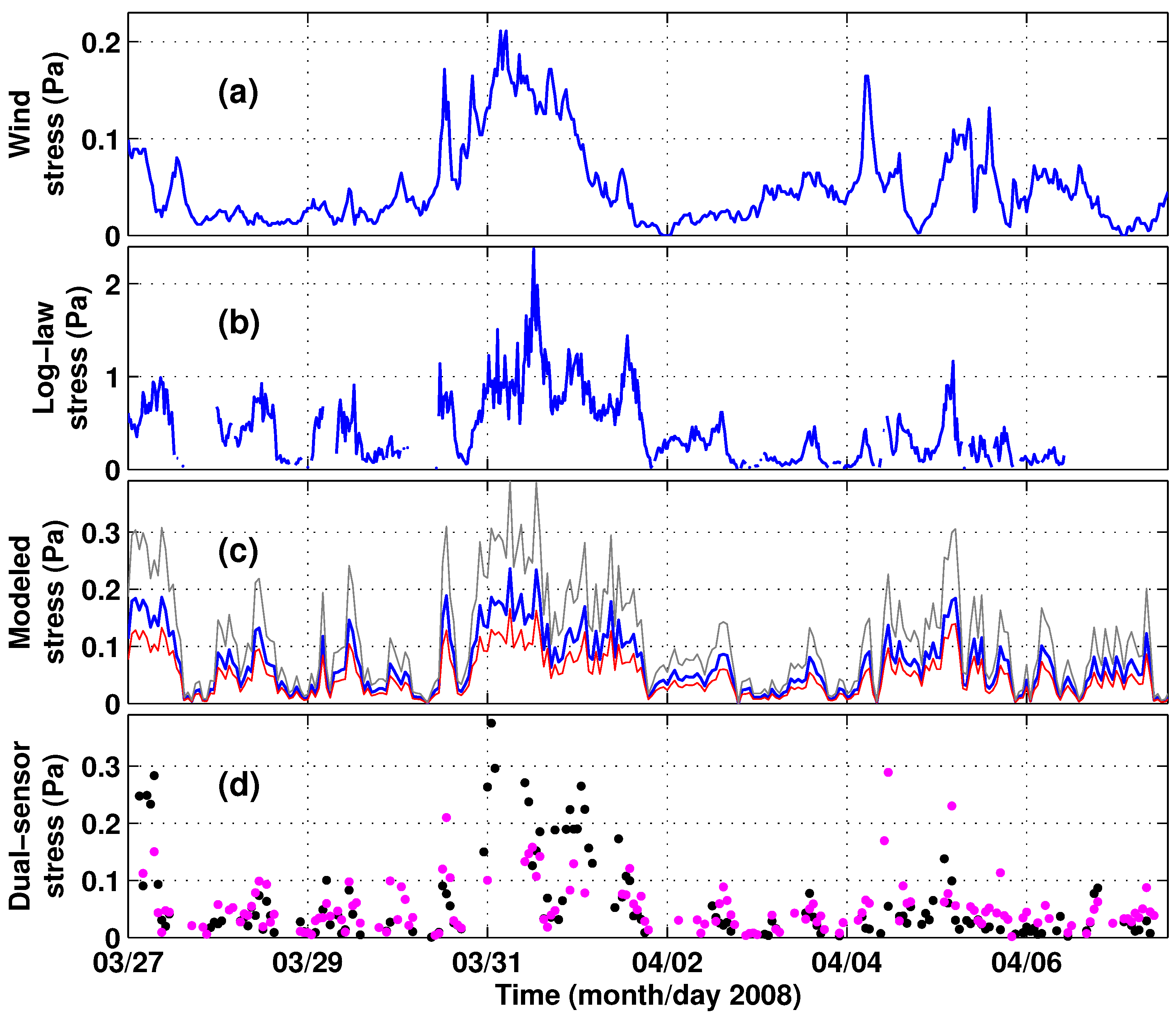
3.2. Stress Estimates

The estimated wind stresses have a maximum of 0.2 Pa (Figure 6a). At the experiment site, which was outside of the surf zone (ratio of significant wave height to depth <0.2 throughout the entire experiment duration), bottom stresses are expected to be the same order of magnitude as the wind stress since the alongshore momentum balance outside the surf zone is expected to be between bottom stress and wind stress [33]. All three methods returned bottom stress estimates that were correlated with each other and also with the wind stress (Figure 6). The stress peaks on 27 March, 31 March, and 4 April all coincide with the periods of relatively strong wave energy (Figure 3), high current speeds (Figure 4b), and near-bed sediment resuspension (Figure 4c). The wind stress, direct estimates of near-bed stress and model results (for all three roughness values tested) are all between 0 and 0.4 Pa (Figure 6a,c,d). The log-law estimates, on the other hand, are consistently greater than all the other estimates (Figure 6b), exceeding 2 Pa on 31 March.
The log-law estimates of bottom stress, wind stress, and model estimates of bottom stress are compared with the direct estimates of near-bed stress (Figure 7). There are about 150 data points in each of these comparisons, since that many measurement bursts provided valid direct stress estimates. Although the direct estimates of stress and the log-law estimates are correlated ( r 2 = 0.43; y intercept of 0.01; Figure 7a), the log-law estimates are greater by a factor of seven. The comparison of the wind stresses with the direct estimates of stress, on the other hand, returns a linear least squares regression slope of 1.03 (with r 2 = 0.38; y intercept of 0.03; Figure 7b). The boundary layer model estimates of bottom stress obtained with k s = 10 - 4 m are correlated with the direct estimates and also return a regression slope close to one (0.93, with r 2 = 0.53; y intercept of 0.004; Figure 7c). Model results obtained with k s = 10 - 5 m underestimate the direct estimates by about 30% on average, and results obtained with k s = 10 - 3 overestimate by about 40%.

4. Discussion

It is known that the indirect estimates of bottom stresses based on the log-law (Equation (1)) are significantly overestimated in stratified boundary layers [20]. To evaluate potential suppression of turbulence by sediment-induced stratification, the suspended-sediment-induced gradient Richardson number is estimated as the ratio of stratification effects to vertical shear effects:
R i = - g ( s - 1 ) ( ϕ / z ) ( u / z ) 2
where g is the gravitational acceleration, s is the specific gravity of sediment, and ϕ is the sediment volume concentration. The stabilizing effects of sediment-induced stratification have been observed to be first-order at R i = 0.03; these effects progressively increase with increasing R i [34,35]. At R i = 0.25, turbulence is significantly suppressed and it can not provide momentum for sediment suspension [34,35]. R i is estimated here based on the velocity and sediment concentration measurements at the elevations of the two OBS-3s. Because R i is found to be greater than 0.03 for the entire duration of the experiment and greater than 0.25 during 60% of the entire duration of experiment (Figure 4d), the overestimation by the log-law is not surprising.
A modified form of the log-law that takes stratification into account is given as [8]:
u ( z ) ¯ u * = 1 κ / ( 1 + A R i f ) l n z z o
where the flux Richardson number is calculated as:
R i f = 0 . 725 [ R i + 0 . 186 - R i 2 - 0 . 316 R i + 0 . 0346 ]
and the value of the coefficient A varies in the literature. Here, the estimations are done based on A = 4.7 and A = 14.7 [5,6,7,8]. A = 4.7 reduced the slope of the comparison between the log-law and Reynolds stress estimates from 7 to 2.8; A = 14.7 reduced it to 1.2 (Figure 7a; green dots and cyan line). This and the R i estimates suggest that the stratification effects on the log-law estimates are strong.
The Reynolds stress estimates here are direct estimates of turbulent vertical transport of horizontal momentum near bed. The sediment-induced stratification discussed above also affects these near-bed stresses [36]. Although the variation of these near-bed stresses versus R i is scattered, it shows an interesting cluster of relatively high stresses at R i < 0 . 25 and relatively small stresses (<0.06 Pa) for R i greater than its critical value of 0.25 (Figure 8). This also indicates the turbulence suppression effect of sediment-induced stratification in the conditions observed here.
Using these direct estimates of near-bed stress (the most fundamental method of the three methods used), the bed drag coefficient is estimated as C d = u * / U c u r 2 through quadratic drag relation. Applying a linear least-square regression between the direct estimates and quadratic estimates (Figure 9) results in average bed drag coefficients of C d = 0.0029 for the East–West component ( r 2 = 0.74) and C d = 0.0023 for the North–South component ( r 2 = 0.66). To get more insight into the variation of bed drag with wave conditions, Figure 10a shows the direct estimates of bed drag as a function of the ratio of current velocity to bottom wave orbital velocity ( U c u r / U o r b ), which is a parameter to quantify the relative importance of waves. For cases with relatively small effect of waves (high U c u r / U o r b ), C d is found to be around 0.0025 (Figure 10a). There is also an overall increasing trend in bed drag with decreasing ratio of current velocity to bottom wave orbital velocity, i.e., relatively strong wave energy (Figure 10a). These results from the muddy study site here are consistent with the previously reported findings in sandy environments [6,15,16,17,19,37]. Recalling that k s = 30 z o , the best model–data agreement obtained with k s = 10 - 4 m (Section 3.2) is also consistent with the z o = 10 - 5 m value reported for a site dominated by silt and clay at San Francisco Bay, USA [38]. However, the observations discussed here indicate no fluid mud formation or muddy bed reworking observed in the study region before [39]. Therefore, how bed drag varies in the presence of much higher concentration fluid mud layers remains to be an open question.
Figure 10b shows the variation of bed drag with Reynolds number, R e = U c u r z / ν . C d has a mostly decreasing trend with increasing R e (i.e., increasing current speed) and it varies within a narrower range as R e increases (Figure 10b), consistent with previous findings [15,20]. To evaluate more directly the effect of wave energy on bed drag, the bed drag estimates are divided into two groups, based on the bottom wave orbital velocities. Cases with bottom orbital velocities greater than the median value of 0.23 m/s (Figure 3e) are defined as high-wave-energy cases; cases with bottom orbital velocities smaller than 0.23 m/s are defined as low-wave-energy cases. High-wave-energy cases are found to be associated with C d values four times greater, on average, than low-wave-energy cases. Wave-induced velocities reaching the muddy bed, which are directly proportional to wave height and period, are enhancing the turbulence near the bed and causing this increase in bed drag [18,40]. It still needs to be stressed that a wave-current interaction formulation implemented in hydrodynamic models without accounting for stress-reducing effects of sediment-induced stratification could be misleading [16,17].

5. Conclusions

The variation of bed drag in a mud-dominated environment under wave action is investigated here, using field observations of waves, currents, and suspended sediment concentration. During diurnal water level changes of 0.6 m average amplitude and moderate wind and wave events at 5 m depth on a mild slope, muddy shelf, winds in excess of 10 m/s generated short waves with 1 m height and longer waves with 0.5 m height. During these windy periods, wind- and tide-induced currents reached 0.5 m/s within the first meter above the bed. Intercomparison of resulting bottom stresses, estimated by three methods (an empirical method, a bottom boundary layer model, and a direct method that uses turbulent velocity fluctuations) is done, followed by the investigation of the variability of direct estimates of bed drag with wave and current conditions.
Although the near-bed structure of current velocities within the first meter above the bed was observed to be logarithmic during the majority of the experiment, the empirical estimates of bottom stress based on log-law are overestimated. This discrepancy was shown to be the result of sediment-induced stratification effects and was significantly reduced by taking these effects into account. The trend and magnitude of the direct estimates of near-bed stress based on the dual-sensor method are similar to the wind stresses. The bottom boundary layer model for combined wave-current flow provides estimates of bottom stress that compare best with these direct estimates when a hydraulic roughness of 10 - 4 m is used in the model. Relatively large and small near-bed stresses are clustered at conditions with R i < 0.25 and R i > 0.25, respectively.
The direct estimates of bed drag coefficients show an overall decrease with increasing current speed, during periods both with and without strong wave energy. The estimated bed drag coefficients are about 0.0025 in relatively strong current flow conditions and increase by a factor of four, on average, in strong wave energy conditions. Although this study’s results on bed drag are from one field site and investigations in other muddy sites may seem necessary, the findings here are consistent with the observations in sandy environments, and they can be used to test the skills of hydrodynamic and sediment transport models in muddy environments by taking into account the effects of both waves and sediment-induced stratification.

Acknowledgments

This research was supported by the Office of Naval Research funding of contracts N00014-07-1-0448, N00014-07-1-0756. Alex Sheremet generously provided full access to the field observations. Cihan Sahin kindly provided a part of the log-law stress analysis. Dan Nowacki, Laura Brothers, and four anonymous reviewers provided valuable feedback which improved the manuscript. Any use of trade, product, or firm names is for descriptive purposes only and does not imply endorsement by the U.S. Government.

Conflicts of Interest

The author declares no conflict of interest.

Abbreviations

ADV
Acoustic Doppler Velocimeter
OBS
Optical Backscatterance Sensor
PC-ADP
Pulse Coherent Acoustic Doppler Profiler

References

  1. Inoue, T.; Glud, R.N.; Stahl, H.; Hume, A. Comparison of three different methods for assessing in situ friction velocity: A case study from Loch Etive, Scotland. Limnol. Oceanogr. 2011, 9, 275–287. [Google Scholar] [CrossRef]
  2. Warner, J.C.; Butman, B.; Dalyander, P.S. Storm-driven sediment transport in Massachusetts Bay. Cont. Shelf Res. 2008, 28, 257–282. [Google Scholar] [CrossRef]
  3. Tennekes, H.; Lumley, J.L. A First Course in Turbulence; The MIT Press: Cambridge, MA, USA, 1972; p. 300. [Google Scholar]
  4. Lueck, R.G.; Lu, Y. The logarithmic layer in a tidal channel. Cont. Shelf Res. 1997, 17, 1785–1801. [Google Scholar] [CrossRef]
  5. Adams, C.E.; Weatherly, G.L. Some effects of suspended sediment stratification on an oceanic bottom boundary layer. J. Geophys. Res. 1981, 86, 4161–4172. [Google Scholar] [CrossRef]
  6. Anwar, H.O. Turbulence measurements in straified and well-mixed estuarine flows. Estuar. Coast. Shelf Sci. 1983, 17, 243–260. [Google Scholar] [CrossRef]
  7. Glenn, S.M.; Grant, W.D. A suspended sediment stratification correction for combined wave and current flows. J. Geophys. Res. 1987, 92, 8244–8264. [Google Scholar] [CrossRef]
  8. Wang, X.H. Tide-induced sediment resuspension and the bottom boundary layer in an idealized estuary with a muddy bed. J. Phys. Oceanogr. 2002, 32, 3113–3131. [Google Scholar] [CrossRef]
  9. Huntley, D.A.; Hazen, D.G. Seabed stresses in combined wave and steady flow conditions on the Nova Scotia continental shelf: Field measurements and predictions. J. Phys. Oceanogr. 1988, 18, 347–362. [Google Scholar] [CrossRef]
  10. Grant, W.D.; Madsen, O.S. Combined wave and current interaction with a rough bottom. J. Geophys. Res. 1979, 84, 1797–1808. [Google Scholar] [CrossRef]
  11. Harris, C.K.; Wiberg, P.L. A two-dimensional, time-dependent model of suspended sediment transport and bed reworking for continental shelves. Comput. Geosci. 2001, 27, 675–690. [Google Scholar] [CrossRef]
  12. Madsen, O.S. Spectral wave-current bottom boundary layer flows. Proc. Int. Conf. Coast. Eng. 1994, 24, 385–398. [Google Scholar]
  13. Benilov, A.Y.; Filyushkin, B.N. Application of methods of linear filtration to an analysis of fluctuations in the surface layer of the sea. Izv. Atmos. Ocean. Phys. 1970, 6, 810–819. [Google Scholar]
  14. Trowbridge, J.H. On a technique for measurement of turbulent shear stress in the presence of surface waves. J. Atmos. Ocean. Technol. 1998, 15, 290–298. [Google Scholar] [CrossRef]
  15. Sternberg, R.W. Friction factors in tidal channels with differing bed roughness. Mar. Geol. 1968, 6, 243–260. [Google Scholar] [CrossRef]
  16. Huntley, D.A.; Huthnance, J.M.; Collins, M.B.; Liu, C.-L.; Nicholls, R.J.; Hewitson, C. Hydrodynamics and sediment dynamics of North Sea sand waves and sand banks. Philos. Trans. R. Soc. Lond. A 1993, 343, 461–474. [Google Scholar] [CrossRef]
  17. Huntley, D.A.; Nicholls, R.J.; Liu, C.; Dyer, K.R. Measurements of the semi-diurnal drag coefficient over sand waves. Cont. Shelf Res. 1994, 14, 437–456. [Google Scholar] [CrossRef]
  18. Signell, R.P.; List, J.H. Effect of wave-enhanced bottom friction on storm-driven circulation in Massachusetts Bay. J. Wtrwy. Port Coast. Ocean Eng. 1997, 123, 233–239. [Google Scholar] [CrossRef]
  19. Bricker, J.D.; Inagaki, S.; Monismith, S.G. Bed drag coefficient variability under wind waves in a tidal estuary. J. Hydraul. Eng. 2005, 131, 497–508. [Google Scholar] [CrossRef]
  20. Sherwood, C.R.; Lacy, J.R.; Voulgaris, G. Shear velocity estimates on the inner shelf off Grays Harbor, Washington, USA. Cont. Shelf Res. 2006, 26, 1995–2018. [Google Scholar] [CrossRef]
  21. Neill, C.F.; Allison, M.A. Subaqueous deltaic formation on the Atchafalaya Shelf, Louisiana. Mar. Geol. 2005, 214, 411–430. [Google Scholar] [CrossRef]
  22. Safak, I.; Allison, M.A.; Sheremet, A. Floc variability under changing turbulent stresses and sediment availability on a wave-energetic muddy shelf. Cont. Shelf Res. 2013, 53, 1–10. [Google Scholar] [CrossRef]
  23. Shaw, W.J.; Trowbridge, J.H. The direct estimation of near-bottom turbulent fluxes in the presence of energetic wave motions. J. Atmos. Ocean. Technol. 2001, 18, 1540–1557. [Google Scholar] [CrossRef]
  24. Nielsen, P. Coastal bottom boundary layers and sediment transport. In Advanced Series on Ocean Engineering; World Scientific: Singapore, 1992; p. 324. [Google Scholar]
  25. Lacy, J.R.; Sherwood, C.R.; Wilson, D.J.; Chisholm, T.A.; Gelfenbaum, G.R. Estimating hydrodynamic roughness in a wave-dominated environment with a high-resolution acoustic Doppler profiler. J. Geophys. Res. 2005, 110. [Google Scholar] [CrossRef]
  26. Sahin, C. Investigation of the variability of floc sizes on the Louisiana Shelf using acoustic estimates of cohesive sediment properties. Mar. Geol. 2014, 353, 55–64. [Google Scholar] [CrossRef]
  27. Kamphuis, J.W. Friction factor under oscillatory waves. J. Wtrwy. Harb. Coast. Eng. Div. 1975, 101, 135–144. [Google Scholar]
  28. Feddersen, F.; Williams, A.J., III. Direct estimation of the Reynolds stress vertical structure in the nearshore. J. Atmos. Ocean. Technol. 2007, 24, 102–116. [Google Scholar] [CrossRef]
  29. Priestley, M.B. Spectral Analysis and Time Series; Academic Press: New York, NY, USA, 1981. [Google Scholar]
  30. Haykin, S. Adaptive Filter Theory; Prentice Hall: New York, NY, USA, 1996; p. 989. [Google Scholar]
  31. Safak, I.; Sheremet, A.; Allison, M.A.; Hsu, T.-J. Bottom turbulence on the muddy Atchafalaya Shelf, Louisiana, USA. J. Geophys. Res. 2010, 115. [Google Scholar] [CrossRef]
  32. Large, W.G.; Yeager, S.G. Diurnal to decadal global forcing for ocean and sea-ice models: The data sets and flux climatologies. In NCAR/TN-460+STR; NCAR: Boulder, CO, USA, 2004; p. 105. [Google Scholar]
  33. Lentz, S.; Guza, R.T.; Elgar, S.; Feddersen, F.; Herbers, T.H.C. Momentum balances on the North Carolina inner shelf. J. Geophys. Res. 1999, 104, 18205–18226. [Google Scholar] [CrossRef]
  34. Soulsby, R.L.; Wainwright, B.L.S.A. A criterion for the effect of suspended sediment on near-bottom velocity profiles. J. Hydraul. Res. 1987, 25, 341–355. [Google Scholar] [CrossRef]
  35. Cacchione, D.A.; Drake, D.E.; Kayen, R.W.; Sternberg, R.W.; Kineke, G.C.; Tate, G.B. Measurements in the bottom boundary layer on the Amazon subaqueous delta. Mar. Geol. 1995, 125, 235–257. [Google Scholar] [CrossRef]
  36. Stacey, M.T.; Monismith, S.G.; Burau, J.R. Observations of turbulence in a partially stratified estuary. J. Phys. Oceanogr. 1999, 29, 1950–1970. [Google Scholar] [CrossRef]
  37. Green, M.O.; McCave, I.N. Seabed drag coefficient under tidal currents in the eastern Irish Sea. Wind-enhanced resuspension in the shallow waters of South San Francisco Bay: Mechanisms and potential implications for cohesive sediment transport. J. Geophys. Res. 1995, 100, 16057–16069. [Google Scholar] [CrossRef]
  38. Brand, A.; Lacy, J.R.; Hsu, K.; Hoover, D.; Gladding, S.; Stacey, M.T. Wind-enhanced resuspension in the shallow waters of South San Francisco Bay: Mechanisms and potential implications for cohesive sediment transport. J. Geophys. Res. 2010, 115. [Google Scholar] [CrossRef]
  39. Safak, I.; Sahin, C.; Kaihatu, J.M.; Sheremet, A. Modeling wave-mud interaction on the central-chenier plain coast, western Louisiana Shelf, USA. Ocean Model. 2013, 70, 75–84. [Google Scholar] [CrossRef]
  40. Green, M.O.; Black, K.P.; Amos, C.L. Control of estuarine sediment dynamics by interactions between currents and waves at several scales. Mar. Geol. 1997, 144, 97–116. [Google Scholar] [CrossRef]
Figure 1. Map of the Atchafalaya Shelf and the bottom isobaths. The "x" indicates the location of the instrumentation platform at about 5 m water depth.
Water 08 00131 g001
Figure 2. Setup of the oceanographic instrumentation. The big white arrow indicates the direction of signal transmission of the Pulse Coherent Acoustic Doppler Profiler (PC-ADP); the thin two-headed arrow indicates the blanking distance between the signal transmissing head and the first measurement bin. The circles denote the sampling volumes of the Acoustic Doppler Velocimeters (ADVs) for velocity measurements; the squares denote the sampling volumes of the ADVs for pressure measurements. OBS-3: Optical Backscatter Sensor.
Water 08 00131 g002
Figure 3. General wind and wave conditions: (a) wind speed and direction (direction indicates where the wind blows towards, measured counter-clockwise from East—i.e., 90 o indicates Northward winds); (b) wave energy spectrum as a function of frequency (in m 2 /Hz; color-scale is logarithmic); (c) peak wave direction (direction indicates where waves propagate towards, measured counter-clockwise from East—i.e., 90 o indicates Northward waves); (d) significant wave height at short-period sea (blue) and long-period swell (red) bands; (e) wave orbital velocity at the bed.
Water 08 00131 g003
Figure 4. (a) Water depth; (b) vertical structure of near-bed current speeds (in m/s; black and dark red dashed lines indicate the levels of suspended sediment concentration (SSC) measurements shown in panel (c); thick white line indicates the bed location); (c) near-bed SSC measurements; (d) estimates of suspended sediment-induced gradient Richardson number (red and green dashed lines indicate R i = 0.25 and R i = 0.03, respectively).
Water 08 00131 g004
Figure 5. Vertical structure of near-bed current measurements as a function of distance above bed in (a) linear scale; and (b) logarithmic scale. The measurements correspond to the peak wind event on 31 March 2008 10:00 with 1 m wave height, 10 m/s winds, and 0.4 m/s currents at 70 cm above bed.
Water 08 00131 g005
Figure 6. Time-series of (a) wind stress; (b) bottom stress estimate based on the log-law of the wall; (c) bottom stress based on the bottom boundary layer model [12] (grey, blue, and red curves correspond to model calculations with k s = 10 - 3 m, 10 - 4 m, 10 - 5 m, respectively); (d) direct estimates of near-bed stress based on the dual-sensor method (black dots denote East–West component of stress; magenta dots denote North–South component of stress).
Water 08 00131 g006
Figure 7. Comparison of the direct estimates of near-bed Reynolds stress with (a) log-law estimates of bottom stress (blue dots and red line correspond to log-law in Equation (1); green dots and cyan line correspond to the log-law estimates that take stratification into account by Equation (4) [8]); (b) wind stress at the sea surface; and (c) bottom stress based on the model [12]. Dashed black lines show the one-to-one relationships; red and cyan lines show the linear least squares regressions.
Water 08 00131 g007
Figure 8. Variation of the direct estimates of near-bed stress with R i . Red dashed line indicates R i = 0.25.
Water 08 00131 g008
Figure 9. Comparison of the direct estimates of near-bed stress with quadratic drag relation. The black and magenta lines are the linear least squares regressions for East–West and North–South components, respectively.
Water 08 00131 g009
Figure 10. Variation of the bed drag coefficient ( C d ) as a function of (a) the ratio of current velocity to bottom wave orbital velocity; and (b) Reynolds number ( R e ). The red dashed lines indicate the canonical value of the bed drag coefficient, C d = 0.0025.
Water 08 00131 g010

