
Characterizing Changes in Streamflow and Sediment Supply in the Sacramento River Basin, California, Using Hydrological Simulation Program—FORTRAN (HSPF)


Abstract
:1. Introduction
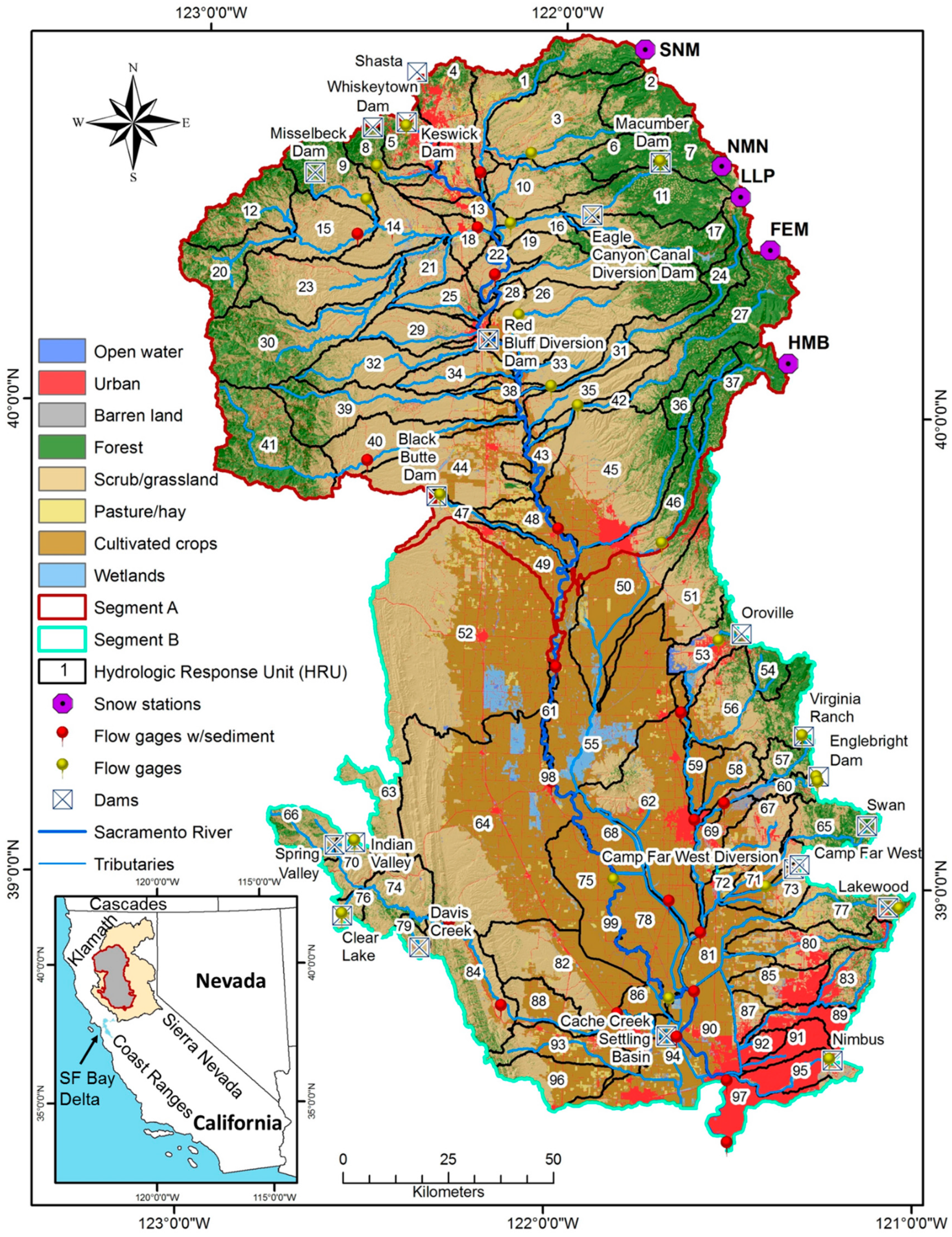
Study Area
2. Methods
2.1. Hydrological Simulation Program—FORTRAN (HSPF)
2.2. HSPF Input
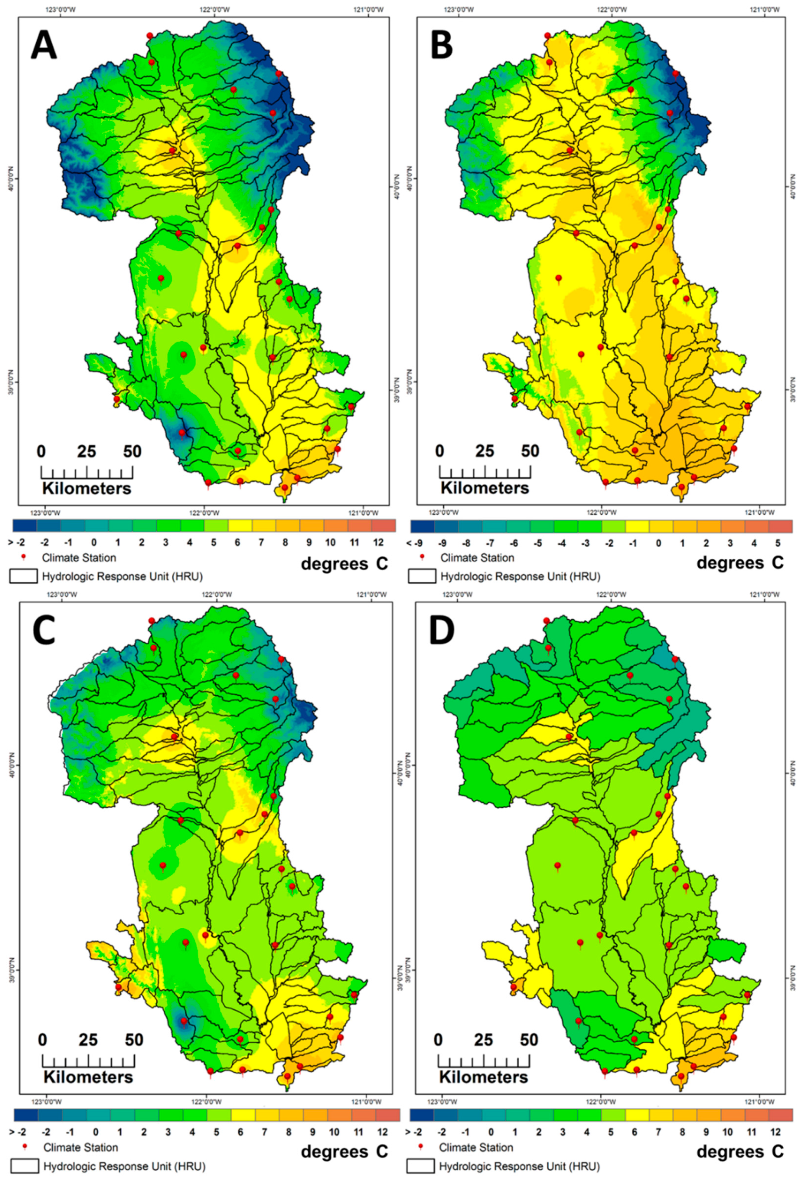
2.2.1. Gridded Meteorological Inputs to HSPF
2.2.2. FTABLE Development
Hydraulic Geometry Method
One-Dimensional Hydraulic Model Method
3. Calibration
3.1. Hydrologic and Sediment Calibration
3.2. Model Performance Evaluation
4. Results
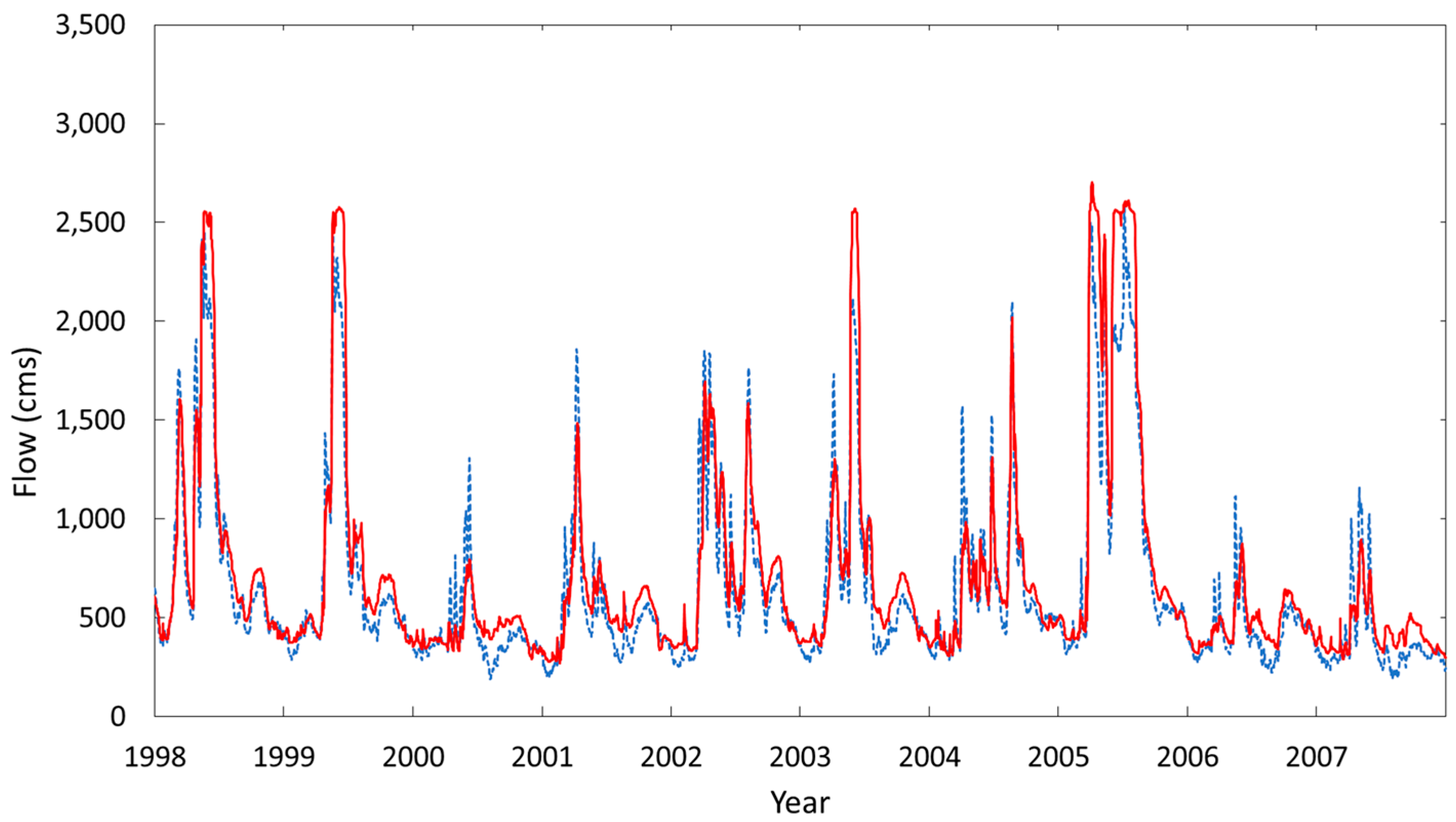
4.1. Hydrology Calibration Results
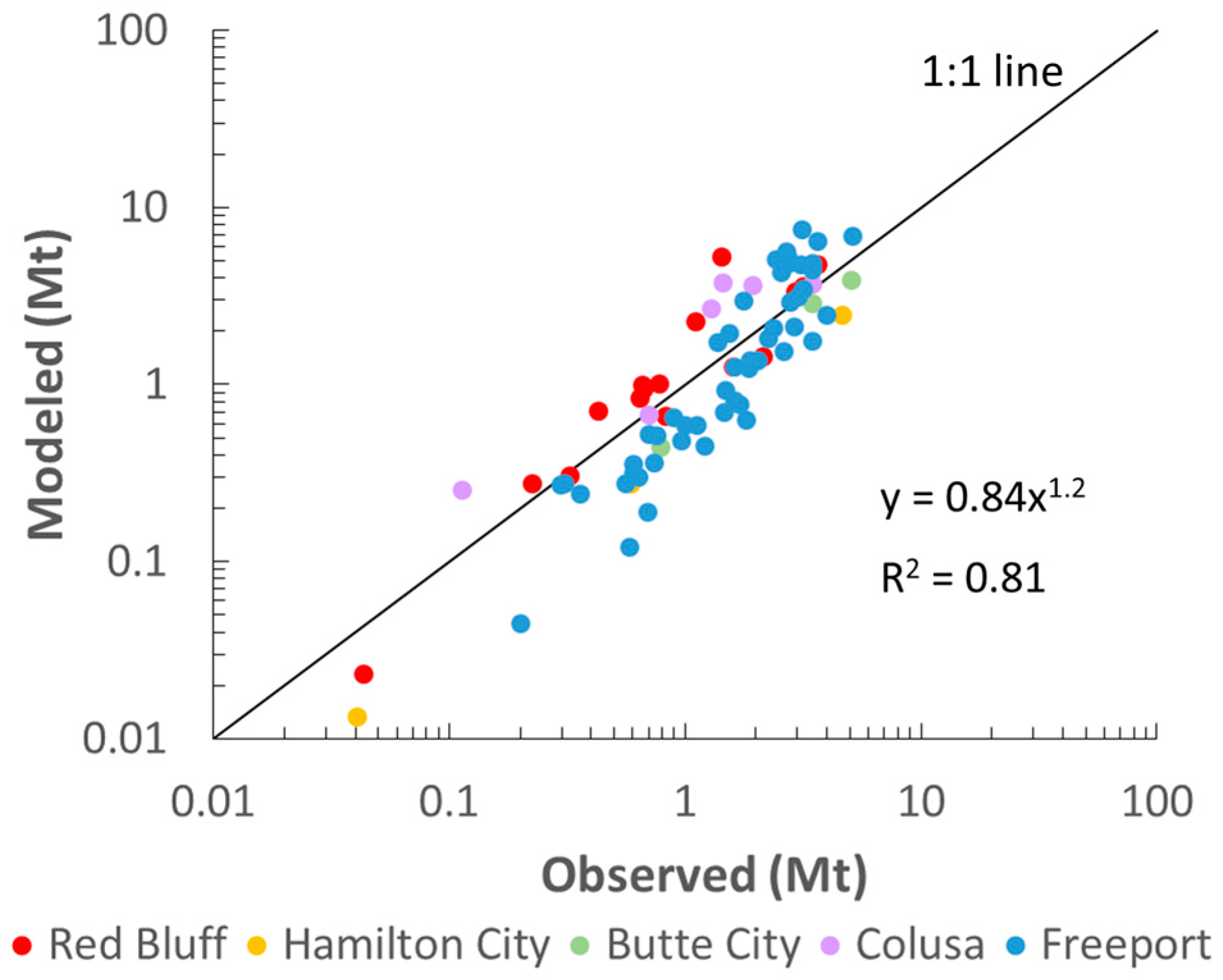
4.2. Sediment Calibration Results
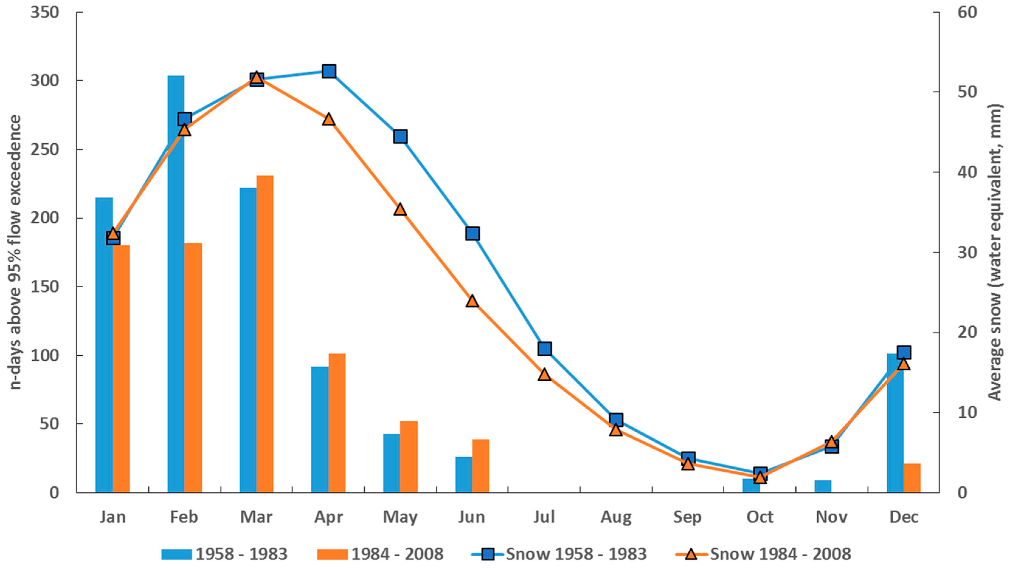
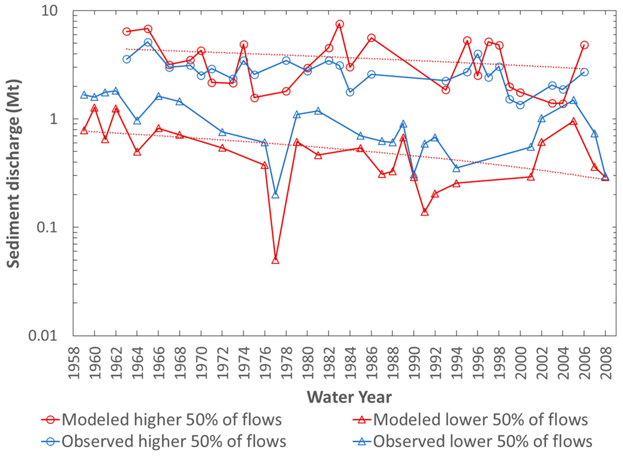
4.3. Historical Trends in Streamflow and Sediment
5. Historical Climate Trends
6. Future Climate Sensitivity Analysis Using Climate Assessment Tool (CAT)
7. Discussion
Model Uncertainty
8. Conclusions
Supplementary Materials
Acknowledgments
Author Contributions
Conflicts of Interest
Abbreviations
| BASINS | Better Assessment Science Integrating Point and Nonpoint Sources program |
| CAT | Climate Assessment Tool |
| CDEC | California Data Exchange Center |
| CIMIS | California Irrigation Management Information System |
| CVFED | Central Valley Floodplain Evaluation and Delineation Program |
| DEM | Digital Elevation Model |
| DWR | California Department of Water Resources |
| FTABLE | Hydraulic Function Table |
| GIDS | Gradient Inverse Distance Squared Interpolation |
| GIS | Geographic Information System |
| HSPF | Hydrological Simulation Program: FORTRAN |
| HRU | hydrologic response unit |
| HSG | Hydrologic Soil Group |
| HUC | USGS Hydrologic Unit (watershed) code |
| IMPLND | Impervious Land Segment |
| INFILT | Index to the Infiltration Capacity of the Soil |
| km | Kilometer |
| m | Meter |
| mm | Millimeter |
| ME% | Mean error percent |
| mg/L | Milligrams per liter |
| Mt | Million metric tons |
| NED | National Elevation Dataset |
| NHD | National Hydrography Dataset |
| NID | National Inventory of Dams |
| NLCD | National Land Cover Dataset |
| NSE | Nash Sutcliffe coefficient of efficiency |
| NWIS | National Water Information System |
| PERLND | Pervious Land Segment |
| PET | Potential Evapotranspiration |
| PRISM | Parameter-elevation Regressions on Independent Slopes Model |
| R | Correlation Coefficient |
| R2 | Coefficient of Determination |
| RCHRES | Modeled Reach or Reservoir |
| SSC | suspended sediment concentration |
| SSURGO | Soil Survey Geographic Database |
| SWE | snow water equivalent |
| UCI | user control input file |
| USGS | United States Geological Survey |
| WY | water year |
References
- Interagency Ecological Program (IEP). Dayflow. 2005. Available online: http://iep.water.ca.gov/dayflow/index.html (accessed on 3 February 2014). [Google Scholar]
- CASCaDE: Computational A of Scenarios of Change for the Delta Ecosystem. Available online: http://cascade.wr.usgs.gov (accessed on 4 April 2016).
- Ganju, N.K.; Schoellhamer, D.H. Decadal-timescale estuarine geomorphic change under future scenarios of climate and sediment supply. Estuar. Coasts 2010, 33, 15–29. [Google Scholar] [CrossRef]
- Wright, S.A.; Schoellhamer, D.H. Trends in the sediment yield of the Sacramento River, California, 1957–2001. San Franc. Estuary Watershed Sci. 2004, 2, 1–14. [Google Scholar]
- Cloern, J.E.; Knowles, N.; Brown, L.R.; Cayan, D.R.; Dettinger, M.D.; Morgan, T.L.; Schoellhamer, D.H.; Stacey, M.T.; van der Wegen, M.; Wagner, R.W.; et al. Projected Evolution of California’s San Francisco Bay-Delta River System in a Century of Climate Change. PLoS ONE 2011, 6, e24465. [Google Scholar] [CrossRef] [PubMed]
- Schoellhamer, D.H.; Wright, S.A.; Drexler, J. A Conceptual model of sedimentation in the Sacramento-San Joaquin Delta. San Franc. Estuary Watershed Sci. 2012, 10, 1–25. [Google Scholar]
- Singer, M.B.; Dunne, T. An empirical-stochastic, event-based program for simulating inflow from a tributary network: Framework and application to the Sacramento River basin, California. Water Resour. Res. 2004, 40. [Google Scholar] [CrossRef]
- Singer, M.B. The influence of major dams on hydrology through the drainage network of the Sacramento River Basin, California. River Res. Appl. 2007, 23, 55–72. [Google Scholar] [CrossRef]
- California Department of Water Resources. California Water Plan Update 2013. Available online: http://www.water.ca.gov/waterplan/docs/cwpu2013/Final/Vol2_SacramentoRiverRR.pdf (accessed on 11 April 2016).
- Bicknell, B.R.; Imhoff, J.C.; Kittle, J.L., Jr.; Donigian, A.S., Jr.; Johanson, R.C. Hydrologic Simulation Program—FORTRAN, User’s Manual for Version 12; U.S. EPA Environmental Research Laboratory: Athens, GA, USA, 2001; pp. 1–755.
- Donigian, A.S.; Bicknell, B.R.; Imhoff, J.C. Hydrological Simulation Program—FORTRAN (HSPF). In Computer Models of Watershed Hydrology; Singh, V.P., Ed.; Water Resources Publications: Highlands Ranch, CO, USA, 1995; pp. 395–442. [Google Scholar]
- Fry, J.A.; Xian, G.; Jin, S.; Dewitz, J.A.; Homer, C.G.; Limin, Y.; Barnes, C.A.; Herold, N.D.; Wickham, J.D. Completion of the 2006 National Land Cover Database for the Conterminous United States. Photogramm. Eng. Remote Sens. 2011, 77, 858–864. [Google Scholar]
- Gesch, D.; Evans, G.; Mauck, J.; Hutchinson, J.; Carswell, W.J. The national map—Elevation. In U.S. Geological Survey Fact Sheet 2009–3053; U.S. Geological Survey: Reston, VA, USA, 2009; p. 4. Available online: http://pubs.usgs.gov/fs/2009/3053/ (accessed on 5 September 2013). [Google Scholar]
- Simley, J.; Carswell, W.J. The National Map—Hydrography; U.S. Geological Survey: Reston, VA USA, 2009; Volume 3054, p. 4.
- Soil Survey Staff. Web Soil Survey. Available online: http://websoilsurvey.nrcs.usda.gov/ (accessed on 5 September 2013).
- Chen, C.W.; Herr, J.W. Comparison of BASINS and WARMF Models: Mica Creek Watershed; Electrcic Power Research Institute: Palo Alto, CA, USA, 2002. [Google Scholar]
- Nigro, J.; Toll, D.; Partington, E.; Ni-Meister, W.; Shihyan, L.; Gutierrez-Magness, A.; Engman, T.; Arsenault, K. NASA-modified precipitation products to improve USEPA nonpoint source water quality modeling for the Chesapeake Bay. J. Environ. Qual. 2010, 39, 1388–1401. [Google Scholar] [PubMed]
- Laroche, A.M.; Gallichand, J.; Lagace, R.; Pesant, A. Simulating atrazine transport with HSPF in an agriculutral watershed. J. Environ. Eng. 1996, 122, 622–630. [Google Scholar] [CrossRef]
- Albek, M.; Ogutveren, U.B.; Albek, E. Hydrological modeling of Seydi Suyu watershed (Turkey) with HSPF. J. Hydrol. 2004, 285, 260–271. [Google Scholar] [CrossRef]
- Kim, S.M.; Benham, B.L.; Brannan, K.M.; Zeckoski, R.W.; Doherty, J. Comparison of hydrologic calibration of HSPF using automatic and manual methods. Water Resour. Res. 2007, 43. [Google Scholar] [CrossRef]
- Tong, S.T.Y.; Sun, Y.; Ranatunga, T.; He, J.; Yang, Y.J. Predicting plausible impacts of sets of climate and land use change scenarios on water resources. Appl. Geogr. 2012, 32, 477–489. [Google Scholar] [CrossRef]
- Hayashi, S.; Murakami, S.; Watanabe, M.; Bao-Hua, X. HSPF simulation of runoff and sediment loads in the Upper Changjiang River Basin, China. J. Environ. Eng. 2004, 130, 801–815. [Google Scholar] [CrossRef]
- Nalder, I.A.; Wein, R.W. Spatial interpolation of climatic normals: Test of a new method in the Canadian boreal forest. Agric. For. Meteorol. 1998, 92, 211–225. [Google Scholar] [CrossRef]
- Flint, L.E.; Flint, A.L. Downscaling future climate scenarios to fine scales for hydrologic and ecological modeling and analysis. Ecol. Process. 2012, 1, 1–15. [Google Scholar] [CrossRef]
- Daly, C.; Halbleib, M.; Smith, J.I.; Gibson, W.P.; Doggett, M.K.; Taylor, G.H.; Curtis, J.; Pasteris, P.P. Physiographically-sensitive mapping of temperature and precipitation across the conterminous United States. Int. J. Climatol. 2008, 28, 2031–2064. [Google Scholar] [CrossRef]
- Priestley, C.H.B.; Taylor, R.J. On the assessment of surface heat flux and evaporation using large-scale parameters. Mon. Weather Rev. 1972, 100, 81–92. [Google Scholar] [CrossRef]
- Bristow, K.L.; Campbell, G.S. On the relationship between incoming solar radiation and daily maximum and minimum temperature. Agric. For. Meteorol. 1984, 31, 159–166. [Google Scholar] [CrossRef]
- Milly, P.C.D.; Dunne, K.A. On the hydrologic adjustment of climate-model projections: The potential pitfall of potential evapotranspiration. Earth Interact. 2011, 15, 1–14. [Google Scholar] [CrossRef]
- U.S. Environmental Protection Agency. BASINS Technical Note 1: Creating Hydraulic Function Tables (FTABLES) for Reservoirs in BASINS; Office of Water: Washington, DC, USA, 2007.
- Leopold, L.B.; Maddock, T., Jr. The Hydraulic Geometry of Stream Channels and Some Physiographic Implications; U.S. Geological Survey Professional Paper 252; U.S. Geological Survey: Reston, VA, USA, 1953; pp. 1–57.
- Gainey, J.; California Department of Water Resources. CVFED Program, Central Valley Floodplain Delineation. Personal communication, 25 February 2014.
- CA DWR Water Supply Information. Available online: http://cdec.water.ca.gov/water_supply.html (accessed on 25 April 2014).
- Fonesca, A.; Ames, D.P.; Yang, P.; Botelho, C.; Boaventura, R.; Vilar, V. Watershed model parameter estimation and uncertainty in data-limited environments. Environ. Model. Softw. 2014, 51, 84–93. [Google Scholar] [CrossRef]
- U.S. Environmental Protection Agency. Estimating Hydrology and Hydraulic Parameters for HSPF: EPA BASINS Technical; Note 6; Office of Water: Washington, DC, USA, 2000; Volume 4305, p. 32.
- Nash, J.E.; Sutcliffe, J.V. River flow forcasting through conceptual models, I, A discussion of principles. J. Hydrol. 1970, 10, 282–290. [Google Scholar] [CrossRef]
- Legates, D.R.; McCabe, G.J. Evaluating the use of “goodness-of-fit” measures in hydrologic and hydroclimatic model validation. Water Resour. Res. 1999, 35, 233–241. [Google Scholar] [CrossRef]
- Donigian, A.J. Watershed model calibration and validation: The HSPF experience. Proc. Water Environ. Fed. 2002, 8, 44–73. [Google Scholar] [CrossRef]
- McKee, L.J.; Ganju, N.K.; Schoellhamer, D.H. Estimates of suspended sediment entering San Francisco Bay from the Sacramento and San Joaquin Delta, San Francisco Bay, California. J. Hydrol. 2006, 323, 335–352. [Google Scholar] [CrossRef]
- U.S. Environmental Protection Agency. BASINS 4.0 Climate Assessment Tool (CAT): Supporting Documentation and User’s Manual; EPA/600/R-08/088F; EPA: Washington, DC, USA, 2009.
- Cayan, D.R.; Maurer, E.P.; Dettinger, M.D.; Tyree, M.; Hayhoe, K. Climate change scenarios for the California region. Clim. Chang. 2008, 87, 21–42. [Google Scholar] [CrossRef]
- Cayan, D.R.; Tyree, M.; Dettinger, M.D.; Hidalgo, H.; Das, T.; Maurer, E.; Bromirski, P.; Graham, N.; Flick, R. Climate Change Scenarios and Sea Level Rise Estimates for California 2008 Climate Change Scenarios Assessment; PIER Research Report, CEC-500-2009-014-D; California Climate Change Center: Sacramento, CA, USA, 2009.
- Dettinger, M.D. Climate change, atmospheric rivers, and floods in California—A multimodel analysis of storm frequency and magnitude changes. JAWRA 2011, 47, 514–523. [Google Scholar] [CrossRef]
- Trenberth, K.E. Conceptual framework for changes of extremes of the hydrological cycle with climate change. Clim. Chang. 1999, 42, 327–339. [Google Scholar] [CrossRef]


| Performance Rating | NSE | R2 | ME% | |||
|---|---|---|---|---|---|---|
| Daily | Monthly | Daily | Monthly | Daily | Monthly | |
| Excellent | ≥0.85 | ≥0.90 | ≥0.85 | ≥0.90 | ≤±10 | ≤±5 |
| Very good | 0.75–0.85 | 0.80–0.90 | 0.75–0.85 | 0.80–0.90 | ±10–±15 | ±5–±10 |
| Good | 0.65–0.75 | 0.70–0.80 | 0.65–0.75 | 0.70–0.80 | ±15–±25 | ±10–±15 |
| Fair | 0.50–0.65 | 0.50–0.70 | 0.50–0.65 | 0.50–0.70 | ±25–±30 | ±15–±25 |
| Poor | <0.50 | <0.50 | <0.50 | <0.50 | ≥±30 | ≥±25 |
| Model Simulation Time Period | NSE | R2 | ME% | ||||
|---|---|---|---|---|---|---|---|
| All Reaches 1 | Sacramento River | All Reaches 1 | Sacramento River | All Reaches 1 | Sacramento River | ||
| Simulation (1958–2008) | daily | 0.69 | 0.90 | 0.79 | 0.92 | −3% | −7% |
| monthly | 0.86 | 0.93 | 0.91 | 0.96 | −7% | −7% | |
| Calibration (1998–2008) | daily | 0.70 | 0.89 | 0.74 | 0.92 | 20% | −10% |
| monthly | 0.78 | 0.92 | 0.84 | 0.96 | 11% | −10% | |
| Validation (1980–1995) | daily | 0.66 | 0.91 | 0.75 | 0.93 | −15% | −11% |
| monthly | 0.83 | 0.94 | 0.88 | 0.97 | −15% | −11% | |
| SSC (mg/L) or Sediment Loads (Tons/Day) | Modeled/Observed | R2 | ME% | ||||
|---|---|---|---|---|---|---|---|
| All Reaches | Sacramento River | All Reaches | Sacramento River | All Reaches | Sacramento River | ||
| Sediment loads | daily | 0.95 | 0.89 | 0.49 | 0.52 | 400% | 21% |
| monthly | 0.97 | 0.91 | 0.72 | 0.74 | 3131% | −9% | |
| SSC | daily | 1.0 | 0.92 | 0.38 | 0.37 | 486% | 55% |
| monthly | 1.0 | 0.95 | 0.64 | 0.56 | 202% | 23% | |
| Location | Variable | 1958–1983 | 1984–2008 | Percent Change |
|---|---|---|---|---|
| Sacramento River at Butte City | precipitation | 476 | 438 | −8% |
| snow | 26.2 | 23.8 | −9% | |
| peak streamflow | 487 | 427 | −12% | |
| Sacramento River at Freeport | precipitation | 481 | 433 | −10% |
| snow | 0.18 | 0.04 | −76% | |
| peak streamflow | 535 | 379 | −29% |
| Scenario | Description | Mean Annual Streamflow (cms) | Mean Annual Sediment Discharge (Tons/Day) | Mean SSC (mg/L) |
|---|---|---|---|---|
| BASE | Reach 97 (1980–2008) | 727 | 8604 | 41.5 |
| Change in Mean Streamflow (Percent) | Change in Mean Sediment Discharge (Percent) | Change in Mean SSC (Percent) | ||
| T1 | Temperature +1.5 °C | −0.5 | −7.7 | −7.9 |
| T2 | Temperature +4.5 °C | −0.7 | −7.9 | −8.3 |
| P1 | Precipitation −10% | +0.5 | +0.5 | +0.6 |
| P2 | Precipitation +10% | +1.9 | +5.1 | +2.2 |
| P3 | Storm magnitude and frequency +10% | +2.6 | +9.0 | +3.3 |
| W1 | Temperature +1.5 °C, precipitation +10% | −0.5 | −7.6 | −7.9 |
| W2 | Temperature +4.5 °C, precipitation +10% | −0.6 | −7.8 | −8.2 |
| W3 | Temperature +1.5 °C, storm magnitude and frequency +10% | −0.6 | −7.7 | −8.0 |
| W4 | Temperature +4.5 °C, storm magnitude and frequency +10% | −0.7 | −7.9 | −8.4 |
| D1 | Temperature +1.5 °C, precipitation −10% | −0.7 | −7.8 | −8.1 |
| D2 | Temperature +4.5 °C, precipitation −10% | −0.8 | −7.9 | −8.5 |
© 2016 by the authors; licensee MDPI, Basel, Switzerland. This article is an open access article distributed under the terms and conditions of the Creative Commons Attribution (CC-BY) license (http://creativecommons.org/licenses/by/4.0/).
Share and Cite
Stern, M.; Flint, L.; Minear, J.; Flint, A.; Wright, S. Characterizing Changes in Streamflow and Sediment Supply in the Sacramento River Basin, California, Using Hydrological Simulation Program—FORTRAN (HSPF). Water 2016, 8, 432. https://doi.org/10.3390/w8100432
Stern M, Flint L, Minear J, Flint A, Wright S. Characterizing Changes in Streamflow and Sediment Supply in the Sacramento River Basin, California, Using Hydrological Simulation Program—FORTRAN (HSPF). Water. 2016; 8(10):432. https://doi.org/10.3390/w8100432
Chicago/Turabian StyleStern, Michelle, Lorraine Flint, Justin Minear, Alan Flint, and Scott Wright. 2016. "Characterizing Changes in Streamflow and Sediment Supply in the Sacramento River Basin, California, Using Hydrological Simulation Program—FORTRAN (HSPF)" Water 8, no. 10: 432. https://doi.org/10.3390/w8100432
APA StyleStern, M., Flint, L., Minear, J., Flint, A., & Wright, S. (2016). Characterizing Changes in Streamflow and Sediment Supply in the Sacramento River Basin, California, Using Hydrological Simulation Program—FORTRAN (HSPF). Water, 8(10), 432. https://doi.org/10.3390/w8100432