1. Introduction
The introduction and enactment of the Water Framework Directive as the main driving frame for the European water policy resulted in a great variety of challenges and complexities for water resources management. This combined with the decrease of water resource availability and quality problems increased the competition for clean water among the various water users and imposed the need to optimize the allocation of available water for each river unit. As the human population continues to grow, water conflicts due to inadequate access and the inappropriate management of scarce freshwater resources force new approaches to long-term water planning and management that incorporate the principles of sustainability and equity [
1,
2,
3]. The basic principles for the allocation of water resources are efficiency, equity and sustainability with the aims of pursuing the maximum benefit for society, the environment and the economy, whilst maintaining fair allocation among regions and people [
4].
A great variety of methodologies has been developed and proposed as thoroughly described in [
1] in order to satisfy the above water management principles and to embody in optimal water allocation the uncertainties of various influencing factors and hydro-system characteristics, such as available water flows, water demands, variations in water supplies, corresponding cost and benefit coefficients and policy regulations. Many optimal water allocation problems require that decisions are made periodically within a time horizon. This can be expressed as two-stage programming (TSP), where a decision is first undertaken before values of random variables are known, and then, after the random events have happened and their values are known, a second decision is made in order to minimize “penalties” that may appear due to any infeasibility [
5]. Various researchers investigated the application of TSP, proposing various advances [
6,
7,
8,
9,
10,
11].
In real-world applications of TSP, some uncertainties are defined as probability density functions (PDFs), while some others as deterministic values followed by post-optimality analyses [
6]. This is explained from the fact that: (1) the quality of information in terms of uncertainty in many practical problems is not good enough to be expressed as PDFs; and (2) the solution of a large TSP model with all uncertain parameters being expressed as PDFs is very difficult and complex, even if these functions are available. Alternatively, methods of post-optimality analysis (such as sensitivity analysis and parametric programming) may be used or best/worst case (BWC) models may be formulated. However, sensitivity analysis is most suitable for problems with few uncertain parameters. If a significant number of parameters is expressed as intervals, various possible combinations of the deterministic values within the intervals should be tested. For large-scale problems, programming this number of combinations may become extremely large [
12]. Despite the fact that parametric programming may help with reducing the number of combinations, it assumes that simultaneous variations occur in the model parameters, which may not be true for real-world applications. In BWC analysis, optimal solutions are determined under best and worst conditions, without necessarily forming stable sets of intervals, and are useful for evaluating the capacity of the system to realize the desired goal. BCW analysis is really a special type of sensitivity analysis for evaluating the responses of model solutions under two extreme conditions.
In order to overcome the above complications in data availability and the solution method, [
6] proposed an inexact two-stage stochastic programming model (ITSP). It is a hybrid method of inexact optimization and TSP [
13] able to handle uncertainties, which cannot be expressed as PDFs. In real-world problems, some uncertainties may indeed exist as ambiguous intervals, since planners and engineers typically find it more difficult to specify distributions than to define fluctuation ranges.
In the present work, an optimal water allocation method under uncertain system conditions is searched for the Alfeios River Basin in Greece. Alfeios is an important river basin in the Peloponnese region in Greece [
14,
15,
16], combining various water uses. These include irrigation, playing a vital social, economic and environmental role associated among others with agricultural income and with water, food and energy efficiency, hydropower generation and drinking water supply. In Alfeios River Basin, as in most Mediterranean countries, water resources management has been focused up to now on an essentially supply-driven approach. It is characterized by a lack of effective operational strategies. Authority responsibility relationships are fragmented, and law enforcement and policy implementations are weak, facts that lead to the difficulty of gathering the necessary data for water resources management or, even worse, to data loss. In some cases, river monitoring, which is crucial for water quantity and quality assessment, if present, is either inefficient with intermittent periods with no measurements or, due to low financial means, the monitoring programs are short and undertaken by a small number of personnel, leading to unreliable and/or short-term data. In this case, some sources of obtaining hydrologic, technical, economic and environmental data required for water resources management come from making additional periodic measuring expeditions, indirectly from expert knowledge, from informal information of the local population or from more general data concerning a wider geographical location (
i.e., country level) from national, European or international databases. Data of this type with a high degree of uncertainty may be easily defined as fluctuation ranges and, therefore, simulated as intervals with lower and upper (deterministic or fuzzy) bounds without the need for any distributional or probabilistic information. Therefore, the ITSP method can be used for optimal water allocation in Alfeios River Basin.
This work is the first part of two papers, which aim at analyzing and applying two similar optimization techniques, in terms of their basic concepts, for optimal water allocation under uncertain system conditions in a real and complex multi-tributary and multi-period water resources system, the Alfeios River Basin. The second methodology, described and discussed in the second paper, extends the ITSP in order to take into account fuzzy boundaries (instead of deterministic) for the variables expressed as intervals, since some intervals are fuzzy in nature. This is called the fuzzy boundary interval-stochastic programming (FBISP) method and is proposed by [
1]. Moreover, the algorithmic process is advanced, including two different solution methods in order to take into account different risk attitudes of decision makers concerning system uncertainties. The reason for organizing these two papers as described above is to facilitate a deeper understanding of this type of methodology through the application of the first method, which is simpler and easier regarding follow up.
The results obtained from this methodology include (1) the optimized water allocation target with a minimized risk of economic penalty from shortages and opportunity loss from spills and (2) an optimized water allocation plan (identification of water allocation and shortages based on the optimized water allocation targets) with a maximized system benefit over a multi-period planning horizon. These types of results are derived as deterministic upper and lower bounds. The system dynamics in terms of decisions for water allocation is mirrored through the consideration of the various equal probability hydrologic scenarios, which have been stochastically generated simultaneously at the positions of the water inflows. The total net system benefits and the benefits and penalties of each main water use for Alfeios are studied and analyzed based on the application of the ITSP method for a baseline scenario and four water and agricultural future scenarios developed within the Sustainability of European Irrigated Agriculture under Water Framework Directive and Agenda 2000 (WADI) project [
17,
18,
19,
20]. These future scenarios cover various possible technical, environmental and socio-economic aspects of the future space for different EU water and agricultural policies, having an impact mainly on agriculture, but also on water resources management. Changes of crop patterns, yields, subsidies, farmer income, variable input costs, market prices per agricultural product, fertilizers and water and hydropower prices are some of the variables described in the narratives of these scenarios, which, in turn, serve as inputs to the optimization algorithm for the evaluation and the estimation of their effect on the water allocation pattern and the system benefits. Finally, for applying the abovementioned optimal water allocation methodology, benefit analysis of each water use, or even better, the determination of economic water value for each water use, identifying the unit benefit and unit penalties of each m
3 of water allocated to each one of the water uses, is undertaken for the Alfeios River.
The paper is organized as follows:
Section 2 includes the presentation of the mathematical background of the ITSP as provided in [
6].
Section 3 describes the Alfeios hydro-system with
Subsection 3.1 focusing on the incorporation of the water inflow dynamics through the simultaneous generation of multiple stochastic hydrologic scenarios at various locations in the Alfeios River Basin.
Section 4 and
Section 5 analyze the benefit and penalty concept of the optimization process for the two main water uses (hydropower and irrigation).
Section 6 analyzes the WADI future scenarios.
Section 7 introduces the formulation of the optimization problem for the Alfeios hydro-system.
Section 8 presents the results and their interpretation, and finally,
Section 9 provides a short discussion and conclusions. In order to facilitate the understanding of the steps of the proposed process and their interactions, a flow chart is also included in
Section 3.1.
2. Mathematical Formulation of the ITSP
The mathematical background of the ITSP model presented in this section is based on [
6]. Let us consider a problem, where a water manager should supply water from various sources to multiple users. The water manager can build the optimization problem as the maximization of the expected value of economic activity in the region. For a water allocation target set for each water user, if this water target is provided, it results in net benefits to the local economy. In the opposite case (nonzero shortages), the desired water target should be obtained from alternative and more expensive water sources, resulting in penalties on the local economy [
5].
Since the total water available is a random variable, the problem can be built as a two-stage stochastic programming model. To solve this problem with linear programming, the distribution of
Q must be approximated by a discrete function. Letting
Q take values
with probability
for
, we have [
5]:
where
= the fixed allocation target for water that is promised to water user
i,
= the maximum allowable allocation amount to user
i,
= the reduction of the net benefit to user
i per unit of water not delivered
,
= the net benefit to user
i per unit of water allocated,
f = the net system benefits,
i = the water user,
m = the number of water users,
= the expected value of a random variable and
is the amount by which water allocation target
is not met when the seasonal flow is
with probability
. The water allocation target (
) and the economic data (
and
) may not be available as deterministic values, but as intervals. This leads to a hybrid ITSP model as follows:
where
,
,
,
,
and
are interval parameters/variables. For example, letting
and
be lower and upper bounds of
, respectively, we have
.
When are known, Model (2) can be transformed into two sets of deterministic submodels, which correspond to the upper and lower bounds of the desired objective function value. This transformation process is based on an interactive algorithm, which is different from normal best/worst case analysis. The resulting solution provides stable intervals for the objective function and decision variables, which can be easily interpreted for generating decision alternatives. The detailed transformation process is as follows.
The first step is to determine values for cost coefficients and decision variables corresponding to the desired bound of the objective function value. For Model (2), is desired, since the objective is to be maximized.
Let
have a deterministic value of
, where
and
. We can then convert Model (2) to:
To put all decision variables at the constraints’ left-hand sides, we can re-write Equations (3b) and (3c) as follows:
For the objective function, we have its upper bound as follows:
Based on Equations (4) and (5), when
approach their upper bounds (
i.e.,
), high benefit could be obtained if the water demands are satisfied, but a high penalty may have to be paid when the promised water is not delivered. Conversely, when
reach their lower bounds (
i.e.,
), we may have a lower benefit, but at the same time, a lower risk of violating the promised targets (and thus, lower penalty). Therefore, it is difficult to determine whether
or
will correspond to the upper bound of the net benefit (
i.e.,
). Thus, if
are considered as uncertain input parameters, existing methods for solving inexact linear programming problems cannot be used directly [
21]. It is proposed that an optimized set of target values can be obtained by having
in Model (5) as decision variables. This optimized set will correspond to the highest possible system benefit given the uncertain water allocation targets.
In the second step, according to [
21], when the constraints’ right-hand sides are also uncertain, the submodel that corresponds to
should be associated with the upper bounds of the right-hand sides (assuming that ≤ relationships exists). Thus, we have the submodel for
as follows:
where
and
are decision variables. The solution for
provides the extreme upper bound of the system benefit given the uncertain inputs of water allocation targets.
In the third step, let
and
be solutions of Model (6). Then, we have the optimized water allocation targets as follows:
In the fourth step according to [
21], we have the submodel for
as follows:
where
are decision variables. Submodels (6) and (8) are deterministic linear programming problems. According to [
22], we have solutions for Model (3) under the optimized water allocation targets as follows:
where
and
are solutions for Submodel (6), and
and
are those of Submodel (8). Thus, the optimal water allocation scheme,
, is defined as the difference of the optimized water allocation targets,
, and the deficits,
:
Solutions under other water allocation target conditions can be obtained by letting be different sets of deterministic values.
3. Description of Alfeios River Basin
The Alfeios River Basin (
Figure 1) has been extensively described in the past [
14,
23,
24]. According to [
14], the Alfeios River is a water resources system of great natural, ecological, social and economic importance for western Greece, since it is the longest watercourse (with a length of 112 km) and has the highest flow rate (absolute maximum and minimum values recorded 2380 m
3/s and 13 m
3/s) in the Peloponnese region in Greece. The main river and its six tributaries represent a significant source of water supply for the region, aiming at delivering and satisfying the expected demands from a variety of water users, including irrigation, drinking water supply, hydropower production and, to a smaller extent, recreation. A plethora of environmental stresses were exerted on its river basin in the last few decades. It drains an area of 3658 km
2. Its annual water yield is estimated to be 2.1 × 10
9 m
3.
The basin constitutes a significant ecosystem and natural resource, providing water, alluvial gravel and lignite to these regions. The soil of the river catchment area consists of alluvial and sandstone deposits, as well as Neogene deposits characterized by discontinuity and heterogeneity. Basin hydrogeology is based on karstic systems, ferrous and manganese content, which makes the groundwater unsuitable for potable use. The prevailing climate in the coastal and flat areas is the marine Mediterranean climate, whereas in the interior, it changes to continental and mountainous types. Precipitation averages 1100 mm annually, ranging from 800 to 1600 mm with occurrences of 80–120 days. The annual basin mean air temperature is 19 °C with a range of variation usually less than 16 °C.
Figure 1.
Alfeios River Basin composed of the main river and the six main tributaries. Representation of the eleven corresponding subcatchments with grey color variations.
Figure 1.
Alfeios River Basin composed of the main river and the six main tributaries. Representation of the eleven corresponding subcatchments with grey color variations.
The primary sector, and mainly the agricultural sector, of the Alfeios region is a significant source of employment and commercial activity. The total agricultural areas constitute 8% of the total agricultural areas of Greece. The mean agricultural area per holding varies between 3.2 and 3.8 ha, characterized as small agricultural units (<5 ha). This sector remains uncompetitive due to high costs, the relatively low product quality, as well as weaknesses in the field of distribution and merchandising. The gross domestic product (GDP) per inhabitant is reaching 51% of the European average index corresponding to one of the lowest among the European regions.
The most important water resource construction works associated with the major water users in the Alfeios River Basin are presented in
Table 1. The main water uses in the basin include: (1) the hydropower production at Ladhon hydropower station (HPS) linked with the Ladhon Dam and reservoir situated in the middle mountainous Alfeios; (2) the agricultural demand of the Flokas scheme linked with the diversion Flokas Dam situated almost 20 km before the discharge of Alfeios into the Kyparissiakos Gulf and very close to Ancient Olympia; (3) the hydropower production at the small HPS at Flokas Dam; and (4) the drinking water supply to the Region of Pyrgos and the neighboring communities from the Alfeios tributary, Erymanthos.
Table 1.
Main water constructions linked to the major water users in the Alfeios River Basin.
Table 1.
Main water constructions linked to the major water users in the Alfeios River Basin.
| Year | Construction Work |
|---|
| 1951 | Gravity Ladhon Dam at Tropaia (reservoir area: 4 km2; storage volume: 46.2 × 10⁶ m3; river basin area: (1) primary 762 km2 and (2) closed secondary 504 km2. |
| 1955 | Hydroelectric power plant of Ladhon (70 GW): 8.6 m downstream of Ladhon Dam (2 vertical Francis turbines with max capacity per turbine: 34.5 MW, 16.9 m3/s). |
| 1967 | Irrigation of the lower Alfeios River Basin (160 km2). |
| Flokas Diversion Dam for irrigation (jumping gravity dam, free spillway; length: 315 m). |
| 2010 | Small hydroelectric power plant at Flokas Dam with max power capacity 6.59 MW (2 Kaplan turbines with max capacity 3.54 MW, 45 m3/s) |
Starting from Ladhon HPS, operated by the Hellenic Public Power Corporation, the two operating purposes of Ladhon reservoir are primarily the satisfaction of irrigation demand at the Flokas irrigation scheme and, secondly, the hydropower production at HPS Ladhon, situated at around 8 km downstream of the Ladhon Dam. Based on these water use priorities, a monthly minimum reservoir level serves as guidance for the operation of the Ladhon HPS. The general rule of thumb is to start at the beginning of January with a minimum level of Ladhon Lake (402 ± 1 m) and then filling up the lake till May with the target reservoir level at 419 ± 1 m, in order to satisfy mainly irrigation demand. It is worth mentioning that the Ladhon River is the most important tributary of the Alfeios River Basin, draining almost one third of the total Alfeios basin area, and it is mainly supplied by karstic sources. Therefore, its contribution to the satisfaction of irrigation demand at Flokas is substantial.
For the application of the ITSP, the upper, lower and maximum allowable bounds of the optimized hydropower production target
(in MWh) at Ladhon are required. These bounds are approximated from the statistical analysis of the monthly time series of hydropower production at Ladhon from 1985–2011. More precisely, it is assumed that the goal of the optimization for this water use is to find the optimized hydropower production target, which ranges between the mean value of the historical time series minus its standard deviation (lower bound) and its mean value plus its standard deviation (upper bound). The maximum allowable hydropower production target is set equal to the maximum monthly registered values of hydropower production (
Table 2).
Focusing on the Flokas irrigation region, the irrigation scheme is connected to the diversion Flokas Dam, draining an area of 3600 km2. It is a jumping gravity dam operating as a free spillway, while water is diverted through side weirs situated (19.7 m) below the elevation of the dam stem (20.7 m). The irrigation water demand extends officially from May to September, whereas in most years, it could be further extended from April up to October, due to the dry climatic conditions. An official agreement for stable water released from the Ladhon HPS in order to satisfy irrigation demand for the months of June, July and August has been arranged between the Hellenic Public Power Corporation and the general irrigation organization responsible for the Flokas irrigation scheme, which is called GOEB Alfeiou-Piniou. In most cases, additional water releases are required. Therefore, the uncertainty of irrigation water demand is not only related to the duration of the irrigation period, but also to the additional unknown short-term extra water demands based on the total irrigation demand and the water availability at Flokas per irrigation month.
The small Flokas HPS is situated directly after the diversion of water from the Flokas Dam and is operated automatically based on the upstream water level. In this way, when the river flow rate is between 9 and 90 m3/s, the entire part of the river flow passes through the Flokas HPS, maintaining the water level of the dam at a stable level. When the river flow rate exceeds 90 m3/s, then the surplus flows over the spillways of Flokas Dam. Whereas for flood water volumes exceeding 300 m3/s, the HPS Flokas closes for security reasons, and the flood volume passes through the spillways of the dam and the opened gateways.
For the application of the ITSP, the upper, lower and maximum allowable bounds of the optimized hydropower production target
(in MWh) at the small Flokas HPS are required. These bounds are approximated also in this case, from the statistical analysis of the monthly time series of hydropower production at Flokas from 2011 to 2015. More precisely, it is assumed that the goal of the optimization for this water use is to find the optimized hydropower production target, which ranges between the mean value of the historical time series minus its standard deviation (lower bound) and its mean value plus its standard deviation (upper bound). The maximum allowable hydropower production target is set equal to the maximum monthly registered values of hydropower production (
Table 3).
Finally, a drinking water supply system for the north and central part of the Region of Hleias has been set into operation in 2013 at Erymanthos River, increasing the complexity of the water allocation pattern. A monthly water flow rate of 0.6 m3/s needs to be diverted from Erymanthos to the water treatment plant and then to the neighboring communities extending up to the city of Pyrgos. Due to the short operation period, this water use, which has the highest priority among the others, is not incorporated into the optimization process as a variable. It is introduced instead as a steady and known water abstraction demand, while for each month, the deficit, if any, based on the considered streamflow at Erymanthos is computed.
Table 2.
Upper (THydroLadhon+) and lower (THydroLadhon−) bound of optimized target for hydropower production and the maximum allowable (THydroLadhonMax) at the hydropower station (HPS) at Ladhon.
Table 2.
Upper (THydroLadhon+) and lower (THydroLadhon−) bound of optimized target for hydropower production and the maximum allowable (THydroLadhonMax) at the hydropower station (HPS) at Ladhon.
| Hydropower Target Limits | Target Limits for Hydropower Production at Ladhon HPS (MWh) |
|---|
| January | February | March | April | May | June | July | August | September | October | November | December | Annual |
|---|
| THydroLadhon− | 11,857 | 12,553 | 11,810 | 11,046 | 11,081 | 8965 | 9077 | 7613 | 5925 | 7387 | 9427 | 8540 | 115,282 |
| THydroLadhon+ | 37,353 | 38,947 | 48,311 | 35,391 | 23,237 | 15,868 | 15,598 | 14,233 | 13,642 | 17,062 | 17,971 | 24,276 | 301,890 |
| THydroLadhonMax | 47,004 | 44,228 | 68,200 | 46,300 | 29,128 | 18,542 | 19,374 | 23,392 | 17,094 | 21,078 | 19,505 | 38,859 | 392,704 |
Table 3.
Upper (THydroFlokas+) and lower (THydroFlokas−) bound of the optimized target for hydropower production and the maximum allowable (THydroFlokasMax) at the HPS at Flokas.
Table 3.
Upper (THydroFlokas+) and lower (THydroFlokas−) bound of the optimized target for hydropower production and the maximum allowable (THydroFlokasMax) at the HPS at Flokas.
| Hydropower Target Limits | Target Limits for Hydropower Production at Flokas HPS (MWh) |
|---|
| January | February | March | April | May | June | July | August | September | October | November | December | Annual |
|---|
| THydroFlokas− | 1244 | 1740 | 2450 | 2045 | 1574 | 437 | 219 | 218 | 232 | 395 | 299 | 1129 | 11,982 |
| THydroFlokas+ | 2379 | 2894 | 3435 | 2840 | 1861 | 773 | 251 | 255 | 571 | 1111 | 1397 | 2097 | 19,865 |
| THydroFlokasMax | 2441 | 3180 | 3536 | 2982 | 1882 | 797 | 257 | 259 | 678 | 1168 | 1662 | 2349 | 21,190 |
Water Inflow Uncertainty for the Alfeios Hydro-System
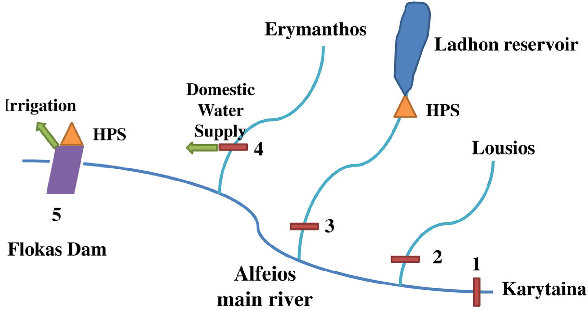
The schematization of the Alfeios River network can be simplified as shown in
Figure 2, including five water inflow locations, where historical time series (rain, temperature and river discharge) are available. For the optimal water allocation problem, one year with a monthly time step (12 stages) is considered. Using the scenario of the tree technique and explicitly considering a number of inflow scenarios, as proposed in [
1], results in an extremely complex scenario tree (taking into account only the first six stages (six months): 2.8 × 10
11 scenarios). For this reason, a different approach for embodying the stochastic uncertainty has been adapted based on the generation of 50 stochastic equal probability hydrologic scenarios simultaneously at the four water inflow location (Cross-section 1–4 in
Figure 2), as is explained below.
The available historical record includes measured time series of mean monthly rain and mean monthly temperature for a 37-year time period, extending from 1959 to 1996, and refers to four main subcatchments of the Alfeios Basin: (1) the Karytaina-Alfeios main river (Cross-section 1 in
Figure 2); (2) the Lousios tributary (Cross-section 2 in
Figure 2); (3) the Ladhon tributary (Cross-section 3 in
Figure 2); and (4) Erymanthos (Cross-section 4 in
Figure 2). For these four subcatchments, time series of measured mean monthly discharge are available, but for a much shorter time period: (1) Karytaina: October 1961–September 1971; (2) Lousios: October 1961–September 1971; (3) Ladhon: October 1996–September 2012; and (4) Erymanthos: October 1961–September 1971.
Figure 2.
The simplified schematic of the Alfeios River Basin.
Figure 2.
The simplified schematic of the Alfeios River Basin.
Based on these hydrologic data, the simple lumped conceptual river basin ZYGOS model [
25,
26], having a similar logic as the HBV model [
27], but requiring less input hydrologic data, has been selected and used for the hydrologic simulation of the four subcatchments. This software models the main hydrological processes of a watershed, using a lumped approach. It implements a conceptual soil moisture accounting scheme, based on a generalization of the standard Thornthwaite model, extended with a groundwater tank. A global optimization procedure, implementing the evolutionary annealing simplex algorithm, is included for the automatic estimation of model parameters, using as the evaluation criterion the coefficient of determination [
28]. It requires rainfall and potential evapotranspiration time series as inputs. The objective function values of the calibration process for the four subcatchments are: (1) Karytaina: 0.892; (2) Lousios: 0.748; (3) Ladhon: 0.906; (4) Erymanthos: 0.854. The Lousios subcatchment discharge is characterized by the high contribution of karstic sources. Moreover, the measured mean monthly discharge record, used for the hydrologic simulation, includes some missing values. Due to these reasons, the calibration efficiency is lower than for the others subcatchments.
The measured rain and temperature time series, as previously mentioned, for 37 years of the four subcatchments serve as inputs into the stochastic software of CASTALIA [
29,
30,
31]. CASTALIA is a system for the stochastic simulation and forecasting of hydrologic variables, including (1) multivariate analysis (for many hydrologic processes, such as rain, temperature and discharge, and geographical correlated locations) and (2) multiple time scales (monthly and yearly) in a disaggregation framework. It enables the preservation of essential marginal statistics up to third order (skewness) and joint second order statistics (auto- and cross-correlations), as well as the reproduction of long-term persistence (Hurst phenomenon) and periodicity. More specifically, an original two-level multivariate scheme was introduced, appropriate for preserving the most important statistics of the historical time series and reproducing characteristic peculiarities of hydrologic processes, such as persistence, periodicity and skewness. At the first stage, the annual synthetic values are generated based on the alternative expression of the backward moving average algorithm [
32] from [
29], resulting in the symmetric moving average (SMA). This modified version extends the stochastic synthesis not only backward, but also forward using the condition of symmetry for the corresponding backward and forward parameters (
aj =
a−j). This model reproduces the long-term persistence and has been further generalized for application to the simultaneous generation of stochastically-dependent multiple variables. This is achieved by generating correlated (multivariable) white noise. At the second stage, the monthly synthetic values are generated placing emphasis on the reproduction of periodicity. A periodic first-order autoregression, abbreviated as PAR (1), model is used, which has been also generalized for multi-variable simulation. The final step is the coupling of the two time scales through a linear disaggregation model [
30].
In the case of Alfeios, the CASTALIA model is applied for the generation of 50 short-time equal probability scenarios for a time length of 10 years and monthly time step (since the future WADI water and agriculture scenarios are based on 10 years after the baseline scenario), simultaneously for the rain and temperature variables at the considered four subcatchments. The stochastically-simulated rain and temperature time series (considering potential evapotranspiration estimated based on the Thornthwaite method) are introduced into the calibrated ZYGOS models for the four subcatchments in order to compute the mean monthly discharges for this 10-year period. The uncertainty from the hydrologic model structure and the parametrization is taken into account through the computation of the standard error between the measured and the simulated water discharge time series. Based on this standard error, the upper bound water inflow time series for all of the hydrologic scenarios (which are used in the f
+ model) and the lower bound (which are used in the f
− model) are created. The steps of this process and the software programs used are presented schematically in the form of a flow chart in
Figure 3.
The last year of each of the 50 stochastic monthly discharge scenarios (since the baseline scenario refers to one year and the future scenarios to the 10th year after the baseline) serve as input inflows into the optimization model for the optimal water allocation of Alfeios River Basin. The monthly discharge at Flokas Dam, which is of interest for the optimization process, since at this position, the available water is diverted to the irrigation canal, is computed as the sum of the four subcatchments multiplied with an area factor in order to enclose also the intermittent subcatchments. As can be seen from
Figure 1, there are some intermittent subcatchments up to Flokas Dam, which have not been included in the described process of the stochastically-computed discharges. The reason for this is the absence of the necessary measured hydrologic data. Their contribution to the sum of the discharges of the four subcatchments is taken into account based on the hydrogeological knowledge for these subcatchments. Ladhon and Lousios subcatchments are mainly supplied by groundwater karstic sources and only limited by the surface runoff. The discharges of the Karytaina and Erymanthos subcatchments are considered to be influenced mainly from the surface runoff. Therefore, the contributions of the unknown intermittent subcatchments to the Flokas discharge, which are also mainly dictated by surface runoff, are roughly approximated by a multiplicative factor based on the drainage area proportion of each subcatchment compared to the Karytaina drainage area. This factor is incorporated into the model increasing the discharge contribution from Karytaina.
Figure 3.
Methodological framework for optimal water allocation of Alfeios River Basin.
Figure 3.
Methodological framework for optimal water allocation of Alfeios River Basin.
4. Unit Benefit and Penalty Analysis for Hydropower Energy
In order to estimate the unit benefit from water allocated to hydropower energy and the corresponding shadow unit penalty, it is worth taking into account the changes in the energy market in Greece based on the illustrative paper of [
33]. As described in this work, until recently, electricity was a monopoly in most countries, including Greece, often government owned, and, if not, highly regulated. As such, electricity prices reflected the government’s social and industrial policy, and any price forecasting that was undertaken was really focused on thinking about underlying costs. In this respect, it tended to be over the longer term, taking a view on fuel prices, technological innovation and generation efficiency. This energy market liberalization has been in effect in Greece since 19 February 2001 with the Law 2773/22.12.1999.
From the above analysis, it is clear that the selling price of hydropower energy, as part of the energy market, has not been fixed and steady since the energy market liberalization. For Greece, it depends on the hourly marginal energy price of the energy system. This price, reflecting the energy price gained by the energy producers, is influenced by, firstly, the combination of the selling price offers and the energy production of each energy production unit and, secondly, by the hourly energy demand of the system. Based on the estimations of the chief engineer responsible for the operation of Ladhon HPS, who was asked to provide minimum and maximum values for the unit benefit from hydropower production at Ladhon under favorable (associated with the maximum benefit from hydropower production) and under unfavorable (associated with the minimum benefit from hydropower production) conditions, an upper and a lower fuzzy boundary interval are defined for the unit benefit from hydropower energy at Ladhon HPS. Due to the absence of the membership function for this fuzzy variable, only the extreme values have been considered in the analysis. Moreover, a study that analyzes statistically the values of the hourly marginal energy prices as provided by the independent Regulatory Authority of Energy (RAE) (which is the organization that controls and regulates the Hellenic energy system) has drawn duration curves of the hourly marginal energy selling prices [
34]. Three zones have been identified based on the operation mode of an energy production unit: base, intermittent and peak. Alternatively, the unit benefit intervals could be derived by making the assumption that the upper bound solution corresponds to the interval values of the intermittent zone of the year with the highest mean hourly marginal energy prices (corresponding to 50% of the time). The lower bound corresponds to the interval of the intermittent zone of the year with the lowest mean hourly marginal energy prices (corresponding to 50% of the time). From the study in [
34], the upper and lower bound intervals based on the above analysis are found to be very close to the estimations of the chief engineer of Ladhon HPS, which are used in this analysis (
Table 4).
Table 4.
Lower and upper fuzzy boundary for the unit benefit (NBHPLadhon and NBHPFlokas) and unit penalty (CHPLadhon and CHPFlokas) for hydropower production at Ladhon and at Flokas.
Table 4.
Lower and upper fuzzy boundary for the unit benefit (NBHPLadhon and NBHPFlokas) and unit penalty (CHPLadhon and CHPFlokas) for hydropower production at Ladhon and at Flokas.
| Variables | NBHPLadhon | NBHPFlokas | CHPLadhon | CHPFlokas |
|---|
| €/MWh | €/MWh | €/MWh | €/MWh |
|---|
| Lower Bound, Minimum | 40 | 87.5 | 120 | 140 |
| Lower Bound, Maximum | 55 | – | 130 | 150 |
| Upper Bound, Minimum | 60 | 80 | 140 | 140 |
| Upper Bound, Maximum | 75 | – | 150 | 150 |
The shadow penalty for the hydropower production at Ladhon is composed of two parts: (1) the penalty due to shortage in comparison to the hydropower production target; and (2) the penalty for the water spilled from the Ladhon Dam, which intends to express the opportunity loss of hydropower energy production. If Ladhon station were the last energy production unit to satisfy the hourly energy demand of the system and, thus, to determine the hourly marginal energy price, then the water lost through spill that could instead satisfy the energy demand is assigned the maximum possible values that the hourly marginal energy price can take. RAE has specified the maximum value (150 €/MWh) that the hourly marginal energy price can obtain. From the hourly selling energy price data by the independent RAE, it is observed that the highest registered value is equal to its maximum possible (150 €/MWh), and this is the value taken as the maximum value of the lower bound interval of the unit penalty at Ladhon. Based again on the estimations of the chief engineer at Ladhon hydropower station, who was asked to provide the highest minimum and maximum values that the Ladhon HPS has gained by selling hydropower energy, the upper and lower bound intervals of
Table 4 for the unit penalty of Ladhon are defined. Following the same concept as described above for the unit benefit based on the duration curves, the unit penalty, assuming now that the intervals of the peak zone correspond to the unit penalty, can be derived. In this case, the derived intervals are lower, ranging from 70 to 110 €/MWh. Since the penalties should be much higher than the unit benefits to force the algorithm to reduce the penalties, the estimations of the chief engineer at Ladhon are used in this study.
The unit benefit and penalty of the small Flokas HPS are approximated in a simpler way, since small hydroelectric power stations are not included in the regulations of the liberalization of the energy market described above. Small HPSs are considered renewable energy systems, and each country is obliged to buy the hydropower energy produced at a steady price. Based on the monthly selling price data of Flokas HPS, the unit benefit is approximated as a single interval (meaning that no upper and lower bound intervals are defined); this value ranges as presented in
Table 4. The unit shadow penalty is approximated as a single interval and is taken as equal to the upper bound solution of the unit penalty of Flokas HPS, as shown in
Table 4.
6. WADI Water and Agriculture Future Scenarios
Under the alternative scenarios of European policy, narratives and quantitative indicator values have been considered as compiled in the WADI Project [
17,
18]. The future agricultural and water scenarios are built on a global and national review of future scenarios developed by the UK “Foresight” program [
14,
15] in an attempt to combine governmental and social preference reflected in water policy. These scenarios have proven to be particularly suitable to explore environmental issues that are defined by processes of long-term and complex change with applications to domains, such as those concerning international trade and water demand. Scenario planning employs qualitative tools to visualize the future. Based on past trends as its starting point, it includes storylines to create representations of alternative worlds that resonate with a range of different individuals. Scenarios are plausible representations of the future based on sets of internally-consistent assumptions, either about relationships and processes of change or about desired end states.
For these future scenarios, first, social and political values and, second, the nature of governance were chosen as the main dimensions of change. Depicting the four scenarios as quartiles of a Cartesian coordinate system, the horizontal axis captures alternative choices made by consumers and policy-makers ranging from the “individual” to the “community”. The vertical governance axis shows alternative structures of political and economic power and decision-making stretching from “interdependence” to “autonomy”.
The four “Foresight” scenarios and the considered agricultural and water scenarios (
Table 11) are connected and briefly described as follows based on [
17,
18]. The world markets scenario is related to private consumption and a highly developed and integrated world trading system. The global sustainability scenario places emphasis on social and ecological values associated with global institutions and trading systems. In comparison to the first scenario, slow, but more equally-distributed growth is considered. Active public policy and international co-operation within the European Union and at a global level are central. The provincial enterprise scenario emphasizes private consumption within the national and regional level to depict local priorities and interests. The dominance of market values is noticed within the national/regional boundaries. The provincial agricultural markets scenario is also characterized by protectionist regimes similar to that under pre-reform Common Agricultural Policy (CAP). People aspire to personal independence and material wealth within a nationally-rooted cultural identity. The local stewardship scenario is focused on strong local or regional governments with emphasis on social values, self-reliance, self-sufficiency and conservation of natural resources and the environment. The local community agriculture scenario emphasizes sustainability at a local level.
Table 11.
Links between Foresight and agricultural future scenarios [
17]. CAP, Common Agricultural Policy; WFD, Water Framework Directive.
Table 11.
Links between Foresight and agricultural future scenarios [17]. CAP, Common Agricultural Policy; WFD, Water Framework Directive.
| Foresight Future Scenarios | Agricultural Policy Scenarios | Intervention Regime |
|---|
| Baseline | Baseline | Moderate: existing price support, export subsidies, with selected agri-environment schemes |
| World Markets | World Agricultural Markets (without CAP) | Zero: free trade, no intervention |
| Global Sustainability | Global Sustainable Agriculture (Reformed CAP) | Low: market orientation with targeted sustainability “compliance” requirements and programs |
| Provincial Enterprise | Provincial Agricultural Markets (Similar to Pre-reform CAP) | Moderate to high: price support and protection to serve national and local priorities for self-sufficiency, limited environmental concern |
| Local Stewardship | Local Community Agriculture | High: locally-defined support schemes reflecting local priorities for food production, incomes and the environment |
| Foresight future scenarios | Water Policy Scenarios | Intervention regime |
| World Markets | Unrestricted Water Markets | Zero: market drivers for water abstraction, use and environment protection, if any |
| Provincial Enterprise | Existing Water Policy (Baseline) | Low: existing water price regimes, including subsidies, with limited environmental controls |
| Global Sustainability | WFD Application | Medium: targeted national programs, environmental targets, cost recovery price. |
| Local Stewardship | Beyond WFD | High: locally-defined support schemes, strict application of protection measures (input use, etc.) |
The WADI project focuses on changes in EU agricultural and water policy as they affect the economic, social and environmental performance of irrigation in the partner countries [
17]. Its aim was to investigate the impacts of policy change on the irrigation sector in Spain, Greece, Italy and the U.K. with a particular focus on the Water Framework Directive and the reform of CAP. The reform of CAP seeks to deliver a market-oriented, internationally-competitive agricultural sector, which supplies quality food for consumers, provides sustainable livelihoods for producers, supports the development of vibrant rural economies and simultaneously protects and enhances the rural environment [
17]. This has been criticized as very challenging, since the agricultural practices and conditions are quite diverse across the EU, and in some cases, the agricultural sector is highly dependent on existing levels of price and income support. The WFD incorporates the concept of sustainable water management, referring to environmental (water quality), social (equal access to water) and economic (water pricing, full cost recovery and liberalization of the world market) dimensions. The baseline is taken as the agricultural policy regime in place in 2001, as determined by CAP at that time. This 2001 baseline is used to provide a relative reference point for the definition of future scenarios. The baseline is also extrapolated to 10 years after 2010 based on predictions (rather than possibilities) of agricultural markets and prices from the EU, the Organization for Economic Co-operation and Development (OCDE) and other sources. The estimates of the main parameters (
Table 12), determined for each future scenario, are used within this paper as inputs in the developed optimal water allocation model based on [
6] under uncertain and vague water system conditions [
16].
Table 12.
Analysis of the Foresight scenarios based on the regional analysis in [
17,
18] Expressed as a percentage of the baseline year at constant values.
Table 12.
Analysis of the Foresight scenarios based on the regional analysis in [17,18] Expressed as a percentage of the baseline year at constant values.
| Parameter Prices | Baseline | World Agricultural Markets | Global Agricultural Sustainability | Provincial Agriculture | Local Community Agriculture |
|---|
| Crop selling prices perceived by the farmers | – | Min | Max | Min | Max | Min | Max | Min | Max |
| Maize | 100 | 85 | 95 | 95 | 105 | 100 | 110 | 100 | 110 |
| Maize area subsidy | 100 | 0 | – | 75 | 85 | 90 | 100 | 85 | 95 |
| Set aside quota | 100 | 0 | – | 95 | – | 100 | – | 105 | – |
| Tomato | 100 | 85 | 95 | 110 | 120 | 100 | 110 | 120 | 130 |
| Potato | 100 | 85 | 95 | 95 | 105 | 105 | 115 | 120 | 130 |
| Watermelons | 100 | 85 | 95 | 95 | 105 | 105 | 115 | 120 | 130 |
| Cotton | 100 | 80 | 90 | 90 | 100 | 85 | 95 | 110 | 120 |
| Cotton subsidy | 100 | 0 | – | 85 | – | 90 | – | 105 | – |
| Olive trees | 100 | 80 | 90 | 85 | 95 | 90 | 100 | 100 | 110 |
| Olive trees area subsidy | 100 | 0 | – | 95 | – | 95 | – | 105 | – |
| Alfalfa | 100 | 80 | 90 | 90 | 100 | 100 | 110 | 110 | 120 |
| Citrus | 100 | 85 | 95 | 95 | 105 | 100 | 110 | 120 | 130 |
| Input prices | – | Min | Max | Min | Max | Min | Max | Min | Max |
| Fertilizers | 100 | 85 | 100 | 140 | 150 | 100 | 110 | 150 | 160 |
| Pesticides | 100 | 110 | 120 | 100 | 105 | 105 | 115 | 95 | 100 |
| Energy | 100 | 85 | 95 | 120 | 130 | 100 | 110 | 130 | 140 |
| Seeds | 100 | 100 | 110 | 110 | 120 | 120 | 130 | 130 | 140 |
| Machinery | 100 | 100 | 115 | 115 | 135 | 100 | 115 | 120 | 140 |
| Contractor services | 100 | 130 | 135 | 120 | 130 | 130 | 140 | 110 | 120 |
| Water prices | 100 | 100 | 110 | 115 | 130 | 100 | 110 | 120 | 140 |
| Irrigation infrastructure | 100 | 100 | 110 | 120 | 130 | 115 | 125 | 130 | 150 |
| Labor | 100 | 90 | 100 | 100 | 110 | 95 | 105 | 110 | 120 |
| Land | 100 | 110 | 120 | 110 | 125 | 100 | 110 | 85 | 95 |
| Other inputs | 100 | 85 | 95 | 125 | 135 | 85 | 95 | 130 | 140 |
| Crop yield changes due to technology | 100 | 110 | 120 | 100 | 115 | 100 | 105 | 85 | 105 |
| Restriction on chemical use | 100 | 130 | 140 | 120 | 130 | 110 | 120 | 100 | 110 |
7. Formulation of the Optimization Problem for the Alfeios River Basin
The goal of this optimization problem is to identify an optimal water allocation target with a maximized economic benefit over the planning period for the Alfeios river basin. Different water allocation targets are related not only to different policies for water resources management, but also to different economic implications (probabilistic penalty and opportunity loss). The objective problem is structured as in Models (3) and (4). The mathematical formulation of the optimization problem is presented thoroughly in the second paper [
44] of this work, which describes and analyzes the FBISP programming method as proposed by [
1].
Article 9 of the EU Water Framework Directive requires Member States to take account of the principle of the recovery of the costs of water services, including environmental and resource costs [
45]. The environmental cost of the water services refers to the environmental consequences from the water use. The EU legislator has effectively assigned the Member States a mathematical task to determine the level of cost recovery achieved for environmental and resource costs. Within the frame of the economic analysis of the water resources systems for Greece, the mean environmental costs per household for Greece has been computed at 33.24 €/year [
46]. For each water body, the environmental costs have been estimated based on the surface water and groundwater quality in terms of pollution from nutrients, nitrate, phosphate and other pollutants. The surface water and groundwater quality for Alfeios River Basin has been evaluated as good, and therefore, the environmental cost is considered to be zero. For this reason, in the valuation of the benefits and costs of each water use, the environmental costs have not been taken into account.
The set of constraints includes: (1) the water volume mass balance for each time period/stage at Ladhon Reservoir, Flokas Dam and Flokas HPS; (2) the minimum and maximum reservoir storage capacity at Ladhon Reservoir; (3) the minimum and maximum release capacity through the turbines for the Ladhon and Flokas HPSs; (4) the minimum environmental flows downstream from the Ladhon and Flokas HPSs; (5) the fish ladder releases at Flokas Dam; (6) the minimum monthly reservoir water level at Ladhon Dam based on its operational curve; (7) the minimum monthly irrigation water demands for the Flokas irrigation scheme; and (8) the steady monthly drinking water abstraction from Erymanthos. Evaporation from the Ladhon Reservoir surface (in m3) is computed by the multiplication of the evaporation rate for Ladhon Reservoir in each time period (in m) with the average of the Ladhon Reservoir areas at the beginning and at the end of each time period. The Ladhon Reservoir area is expressed as a linear function of reservoir water volume as explained in the next paragraph.
In the optimization problem, there are some nonlinear equations, such as the relationship between water flowing through the turbines and the hydropower energy produced. In order to introduce them into the linear programming algorithm, their linear regression equations are considered. The uncertainty resulting from this simplification has not been considered in the process, but it is worth mentioning that in all cases, the R2 of the linear regression takes values ≥0.9. In the Alfeios optimization problem, the following relationships have been linearized: (1) the surface reservoir area (km2) and reservoir water volume (m3) relationship of Ladhon Reservoir; (2) the water flowing through the turbines (named the water volume released) (m3) and hydropower energy produced (MWh) relationship at Ladhon HPS and at Flokas HPS; (3) the unit benefit for each m3 water allocated to irrigation (€/m3) and water volume allocated to irrigation (m3) relationship for the Flokas irrigation scheme; and (4) the unit penalty for each m3 irrigation water deficit (€/m3) and irrigation water deficit (m3) relationship for the Flokas irrigation scheme.
The uncertain variables are: the coefficient of the objective function, including the unit benefits and penalties from the hydropower production of Ladhon (€/MWh) in
Table 4, from the hydropower of Flokas (€/MWh) in
Table 4 and from the Flokas irrigation (€/m
3) in
Table 7 and the initial water level of Ladhon Reservoir at Stage 0 (m
3) (12,362,644.01, 26,783,729.12). The incorporation of water inflow uncertainty has been approximated through the generation of 50 stochastic equal probability scenarios simultaneously at all water inflow locations by using CASTALIA stochastic simulation and forecasting software, as analyzed in the previous section.
For the application of ITSP, the uncertain variables, which are expressed as intervals, should have deterministic bounds. For this reason, the mean values of the minimum and maximum value of the upper and the lower bounds are considered as presented in
Table 13. The initial water level of Ladhon Reservoir at Stage 0 is also set equal to its mean value and is no longer considered as uncertain for the application of ITSP.
Table 13.
Unit benefit and unit penalties for water allocation to the three water users for the application of the inexact two-stage stochastic programming model (ITSP) and uncertain variable combinations for the upper bound solution f+ and the lower bound solution f−.
Table 13.
Unit benefit and unit penalties for water allocation to the three water users for the application of the inexact two-stage stochastic programming model (ITSP) and uncertain variable combinations for the upper bound solution f+ and the lower bound solution f−.
| Variables | NBHPLadhon | NBHPFlokas | NBIrrigationFlokas | CHPLadhon | CHPFlokas | CIrrigationFlokas |
|---|
| €/MWh | €/MWh | €/m3 | €/MWh | €/MWh | €/m3 |
|---|
| Minimum | 47.5 | 80 | 0.171 | 125 | 140 | 1.114 |
| Maximum | 67.5 | 87.5 | 0.196 | 145 | 150 | 1.91 |
| f+ | 67.5 | 87.5 | 0.196 | 125 | 140 | 1.114 |
| f− | 47.5 | 80 | 0.171 | 150 | 150 | 1.91 |
The unit benefit and unit penalty for irrigation for the baseline and the future scenarios are given in
Table 14.
Table 14.
Unit benefit (NBIrrigationFlokas) and unit penalties (CIrrigationFlokas) for water allocated to irrigation, €/m3, for the baseline and the future scenarios for the application of the ITSP.
Table 14.
Unit benefit (NBIrrigationFlokas) and unit penalties (CIrrigationFlokas) for water allocated to irrigation, €/m3, for the baseline and the future scenarios for the application of the ITSP.
| Unit benefit and Penalty | Baseline | FS1 | FS2 | FS3 | FS4 |
|---|
| NBIrrigationFlokas €/m3 | 0.171 | 0.196 | 0.132 | 0.212 | 0.227 | 0.268 | 0.234 | 0.296 | 0.258 | 0.363 |
| CIrrigationFlokas €/m3 | 1.114 | 1.91 | 1.57 | 3.458 | 1.098 | 2.245 | 1.111 | 2.191 | 1.096 | 2.373 |
8. Results
For each of the two models solved (f+ and f−) as described above, (1) the optimized water allocation target for each time stage (the twelve months of the examined year), as well as for total annual (as the summation of the values of the twelve time stages), (2) the probabilistic shortages and allocations for each one of the 50 hydrologic scenarios and for each of the three water users for each time stage (the twelve months of the examined year), as well as for the total annual (as the summation of the values of the twelve time stages) and (3) the total benefits and the benefits and penalties for each of the three water users are derived. The analysis of these results concerns the baseline scenario and also the effect of the different water and agriculture policies represented by the four future scenarios on the benefits and penalties of the baseline scenario.
The results derived from this methodology for the objective function, meaning the net benefits from the water allocated to the three water users, as well as the non-zero water allocation and shortages are expressed as intervals. The resulting solutions provide stable intervals for the objective function and decision variables, which can be easily interpreted for generating decision alternatives [
6]. The values of
and
depict the two extreme conditions of the total net benefit of the system, ranging between their upper and lower bounds. This solution process may result in extremely high system benefits under favorable conditions, but it may also lead to high penalties in the case of shortages in relation to the corresponding water allocation targets. This uncertainty produces broad intervals between the upper and the lower bounds of
.
From the solution of the model f
+ for the Alfeios River Basin, the optimized water allocation targets for the three water uses are computed and presented in
Table 15. Based on the
yi values, the monthly optimized water allocation target values for irrigation are equal to the maximum possible allocation, TIrrigation
+. For the hydropower production at Ladhon, the monthly optimized hydropower production target values are equal to the maximum possible, THydroLadhon
+, for all months except June (60% of its maximum value), September (67% of its maximum value), October (23% of its maximum value) and November (58% of its maximum value). For the hydropower production at Flokas, the monthly optimized hydropower production target values are equal to the maximum possible allocation, THydroLadhon
+, for all months, except May (89% of its maximum value) and June (99% of its maximum value). From these results, it is concluded that the highest priority is set to irrigation, since it has the highest unit benefit, but at the same time also the highest unit penalty. The next two priorities are set to the hydropower production at Flokas, and last, but not least, to the hydropower production at Ladhon, which has the smallest unit benefit.
Table 15.
Monthly and annual optimized water allocation targets.
Table 15.
Monthly and annual optimized water allocation targets.
| Title? | Optimized Water Allocation Targets |
|---|
| Irrigation m3 | Hydropower at Ladhon MWh | Hydropower at Flokas MWh |
|---|
| yi | | yi | | yi |
|---|
| t = 1, January | 0 | 1 | 37,353 | 1 | 2379 | 1 |
| t = 2, February | 0 | 1 | 38,947 | 1 | 2894 | 1 |
| t = 3, March | 16,070,400 | 1 | 48,311 | 1 | 3435 | 1 |
| t = 4, April | 15,552,000 | 1 | 35,391 | 1 | 2840 | 1 |
| t = 5, May | 16,070,400 | 1 | 23,237 | 1 | 1828 | 0.89 |
| t = 6, June | 31,104,000 | 1 | 15,868 | 1 | 770 | 0.99 |
| t = 7, July | 32,140,800 | 1 | 12,997 | 0.60 | 251 | 1 |
| t = 8, August | 32,140,800 | 1 | 14,233 | 1 | 255 | 1 |
| t = 9, September | 15,552,000 | 1 | 11,084 | 0.67 | 571 | 1 |
| t = 10, October | 16,070,400 | 1 | 9618 | 0.23 | 1111 | 1 |
| t = 11, November | 0 | 1 | 14,395 | 0.58 | 1397 | 1 |
| t = 12, December | 0 | 1 | 24,276 | 1 | 2097 | 1 |
| Annual | 174,700,800 | – | 28,5710 | – | 19,828 | – |
The optimized water allocation targets are the same also for the four WADI future scenarios. The four WADI future scenarios mirror four different possible water and agricultural policy alternatives in comparison to the baseline scenario, which may have an impact on the optimal water allocation. The differences between the future scenarios include, among others, changes of hydropower energy prices, water prices, selling prices of the agricultural products, yield functions, subsidies, farmer income variable costs, labor and fertilizers. Therefore, the main impact of these scenarios is on the net benefits from the system.
In
Table 16, (1) the total maximized net benefits (€) based on the optimized water allocation targets for the three water uses and (2) the maximized benefits (€) and penalties (€) of each water use for the baseline and the future scenarios are presented. The total maximized net benefits of the hydro-system range between (131,565,871, 99,636,682) for the baseline scenario. From this table, it is verified that for the lower bound model f
−, the benefits are lower and the penalties are higher in comparison to the corresponding results from the upper bound model f
+. The ratios of the benefits and penalties from the four future scenarios in comparison to the baseline are also given in
Table 16. It is worth mentioning that the highest increase of the total system benefits is observed for the local stewardship scenario ranging from 52% to 59% for the total net system benefit (objective function value). The only decrease of the net benefits compared to the benefits of the baseline scenario occurs for the world market scenario (9%–24%).
Table 16.
Total net benefit (€) from all water uses. OF, objective function.
Table 16.
Total net benefit (€) from all water uses. OF, objective function.
| WADI Scenarios | OF Type | Total Benefit | Benefit HPLadhon | Penalty HPLadhon | Benefit Irrigation | Penalty Irrigation | Benefit HPFlokas | Penalty HPFlokas |
|---|
| Baseline | f+ | 131,565,871 | 19,285,425 | 8,036,313 | 34,293,767 | 487,058 | 86,748,308 | 238,257 |
| f− | 99,636,682 | 13,571,225 | 14,789,609 | 29,856,367 | 7,001,907 | 79,312,739 | 1,312,133 |
| FS1 | f+ | 119,497,839 | 16,392,611 | 6,830,866 | 37,088,980 | 686,429 | 73,736,062 | 202,518 |
| f− | 75,543,823 | 11,535,541 | 12,571,167 | 22,955,685 | 12,676,750 | 67,415,828 | 1,115,313 |
| FS2 | f+ | 183,150,169 | 26,999,594 | 11,250,839 | 46,767,404 | 480,063 | 121,447,631 | 333,560 |
| f− | 138,922,202 | 18,999,715 | 20,705,452 | 39,657,082 | 8,229,990 | 111,037,834 | 1,836,986 |
| FS3 | f+ | 148,932,442 | 19,285,425 | 8,036,313 | 51,659,027 | 485,747 | 86,748,308 | 238,257 |
| f− | 109,560,299 | 13,571,225 | 14,789,609 | 40,810,107 | 8,032,030 | 79,312,739 | 1,312,133 |
| FS4 | f+ | 209,558,476 | 28,928,137 | 12,054,470 | 63,398,920 | 479,188 | 130,122,462 | 357,385 |
| f− | 151,459,561 | 20,356,837 | 22,184,413 | 44,985,456 | 8,699,228 | 118,969,108 | 1,968,199 |
| FS1/Baseline | f+ | 91% | 85% | 85% | 108% | 141% | 85% | 85% |
| f− | 76% | 85% | 85% | 77% | 181% | 85% | 85% |
| FS2/Baseline | f+ | 139% | 140% | 140% | 136% | 99% | 140% | 140% |
| f− | 139% | 140% | 140% | 133% | 118% | 140% | 140% |
| FS3/Baseline | f+ | 113% | 100% | 100% | 151% | 100% | 100% | 100% |
| f− | 110% | 100% | 100% | 137% | 115% | 100% | 100% |
| FS4/Baseline | f+ | 159% | 150% | 150% | 185% | 98% | 150% | 150% |
| f− | 152% | 150% | 150% | 151% | 124% | 150% | 150% |
The results for the annual shortage and the annual allocation (
Table 17) for irrigation, as computed by the optimization algorithm for the 50 hydrologic equal probability scenarios, are provided. In most hydrologic scenarios, the water allocation is equal to the desired target, therefore resulting in zero annual shortages. There are only a few hydrologic scenarios with nonzero shortages. Among these scenarios, Hydrologic Scenario 19 is the worst shortage condition. In this case, the annual water allocation interval is (114,297,023, 1,528,400,127) in m
3 and the corresponding shortage interval (21,860,788, 60,403,777) in m
3. By computing the shortage to target ratio, which varies from 12.5% to 34.6%, it is indicated that the shortage is serious. In this case, if the farmers do not have an alternative water source (such as pumping water from groundwater or wastewater reuse), a yield reduction is highly possible, which is introduced into the objective function as a penalty for irrigation. The solutions of water shortage and allocation for the other hydrologic scenarios can be accordingly interpreted.
Table 17.
Annual water allocation and shortage for irrigation at Flokas (m3).
Table 17.
Annual water allocation and shortage for irrigation at Flokas (m3).
| Hydro Scenarios | Allocation for Irrigation at Flokas m3 | Shortage for Irrigation at Flokas m3 |
|---|
| f+ | f− | f+ | f− |
|---|
| 1 | 174,700,800 | 160,234,637 | 0 | 14,466,163 |
| 2 | 174,700,800 | 174,700,800 | 0 | 0 |
| 3 | 174,700,800 | 174,700,800 | 0 | 0 |
| 4 | 174,700,800 | 174,700,800 | 0 | 0 |
| 5 | 174,700,800 | 174,700,800 | 0 | 0 |
| 6 | 174,700,800 | 172,492,722 | 0 | 2,208,078 |
| 7 | 174,700,800 | 174,700,800 | 0 | 0 |
| 8 | 174,700,800 | 174,700,800 | 0 | 0 |
| 9 | 174,700,800 | 174,618,224 | 0 | 82,576 |
| 10 | 174,700,800 | 174,700,800 | 0 | 0 |
| 11 | 174,700,800 | 174,700,800 | 0 | 0 |
| 12 | 174,700,800 | 165,262,713 | 0 | 9,438,087 |
| 13 | 174,700,800 | 174,700,800 | 0 | 0 |
| 14 | 174,700,800 | 162,728,220 | 0 | 11,972,580 |
| 15 | 174,700,800 | 174,700,800 | 0 | 0 |
| 16 | 174,700,800 | 174,700,800 | 0 | 0 |
| 17 | 174,700,800 | 174,700,800 | 0 | 0 |
| 18 | 174,700,800 | 174,700,800 | 0 | 0 |
| 19 | 152,840,012 | 114,297,023 | 21,860,788 | 60,403,777 |
| 20 | 174,700,800 | 174,700,800 | 0 | 0 |
| 21 | 174,700,800 | 174,700,800 | 0 | 0 |
| 22 | 174,700,800 | 174,700,800 | 0 | 0 |
| 23 | 174,700,800 | 174,700,800 | 0 | 0 |
| 24 | 174,700,800 | 174,700,800 | 0 | 0 |
| 25 | 174,700,800 | 174,700,800 | 0 | 0 |
| 26 | 174,700,800 | 174,700,800 | 0 | 0 |
| 27 | 174,700,800 | 174,700,800 | 0 | 0 |
| 28 | 174,700,800 | 174,637,545 | 0 | 63,255 |
| 29 | 174,700,800 | 150,955,791 | 0 | 23,745,009 |
| 30 | 174,700,800 | 174,700,800 | 0 | 0 |
| 31 | 174,700,800 | 174,700,800 | 0 | 0 |
| 32 | 174,700,800 | 174,700,800 | 0 | 0 |
| 33 | 174,700,800 | 174,700,800 | 0 | 0 |
| 34 | 174,700,800 | 174,700,800 | 0 | 0 |
| 35 | 174,700,800 | 174,700,800 | 0 | 0 |
| 36 | 174,700,800 | 160,776,364 | 0 | 13,924,436 |
| 37 | 174,700,800 | 174,700,800 | 0 | 0 |
| 38 | 174,700,800 | 174,700,800 | 0 | 0 |
| 39 | 174,700,800 | 174,700,800 | 0 | 0 |
| 40 | 174,700,800 | 174,700,800 | 0 | 0 |
| 41 | 174,700,800 | 151,565,626 | 0 | 23,135,174 |
| 42 | 174,700,800 | 174,700,800 | 0 | 0 |
| 43 | 174,700,800 | 174,700,800 | 0 | 0 |
| 44 | 174,700,800 | 158,189,688 | 0 | 16,511,112 |
| 45 | 174,700,800 | 174,700,800 | 0 | 0 |
| 46 | 174,700,800 | 167,355,061 | 0 | 7,345,739 |
| 47 | 174,700,800 | 174,700,800 | 0 | 0 |
| 48 | 174,700,800 | 174,700,800 | 0 | 0 |
| 49 | 174,700,800 | 174,700,800 | 0 | 0 |
| 50 | 174,700,800 | 174,700,800 | 0 | 0 |
The results for the annual shortage and the annual hydropower production at Flokas and Ladhon, as computed by the optimization algorithm for the 50 hydrologic equal probability scenarios, are presented in
Table 18. In most hydrologic scenarios, the hydropower production is not equal to the desired target, therefore resulting in nonzero annual shortages for both hydropower stations. There are only a few hydrologic scenarios with zero shortages. Among these scenarios, Hydrologic Scenario 19 is the worst shortage condition for the HPS at Ladhon. In this case, the annual hydropower production interval is (25,943, 45,515) in MWh and the corresponding shortage interval (240,195, 259,767) in MWh. By computing the shortage to target ratio, which varies from 84% to 90.9%, it is indicated that the shortage is serious. Hydrologic Scenario 28 is the worst shortage condition for the small HPS at Flokas. In this case, the annual hydropower production interval is (5191, 12,729) in MWh and the corresponding shortage interval from the desired target (7099, 14,637) in MWh. By computing the shortage to target ratio, which varies from 35.8% to 73.8%, it is indicated that the shortage is serious.
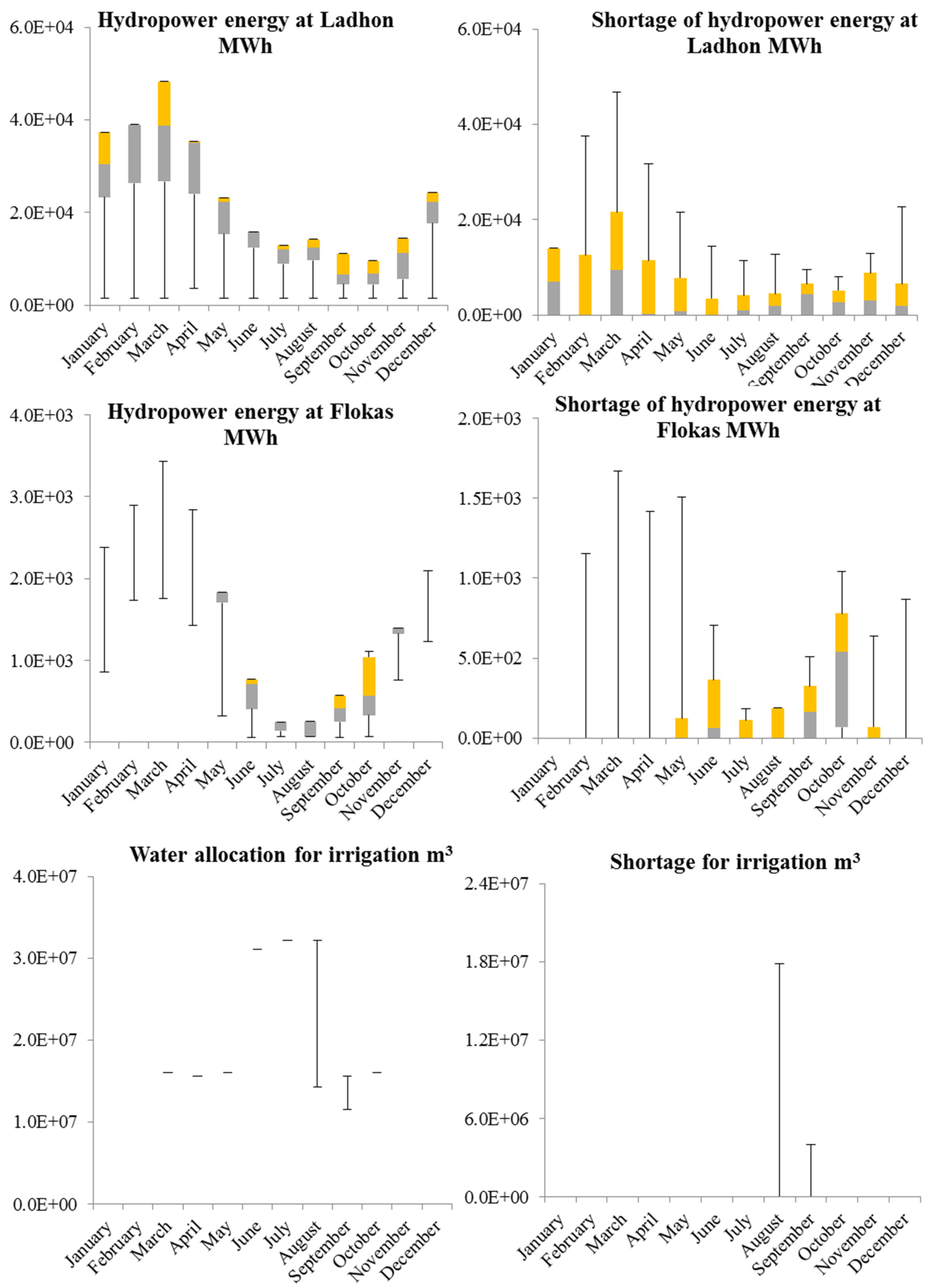
The statistical analysis of the monthly water allocations and corresponding shortages (due to the high amount of data) for all stages (twelve months) for the 50 hydrologic scenarios is graphically presented in
Figure 4 for the model f
+ and the baseline scenarios through the use of box plots for Alfeios River Basin in western Greece. Some very interesting comments from these figures are given as follows. For the irrigation, the shortages take place in August and September. This can be explained by the facts that the flow rate at Flokas Dam for these two months is very low and that the irrigation demand is increased. For the hydropower production at Ladhon, the highest shortages occur from January–April (with the highest in March). This can be justified by the fact that the highest priority in terms of the satisfaction of the desired target is set on irrigation. In order to satisfy the irrigation demand, which starts mainly from May (having only a very low demand also in April), the water volume flowing into the Ladhon Reservoir from December–April should be stored and not released. Therefore, there is a conflict between the two uses for this time period. Finally, for the hydropower production at Flokas, the highest shortages occur from June–October (with the highest in October), which is the irrigation period, revealing a conflict between the two uses. The operation of the small HPS at Flokas is only set in operation after having satisfied irrigation, and this leads to the shortages for these months.
Table 18.
Annual hydropower production and shortage at the HPS at Ladhon and at Flokas (MWh).
Table 18.
Annual hydropower production and shortage at the HPS at Ladhon and at Flokas (MWh).
| Hydro Scenarios | Hydropower at Flokas MWh | Shortage for Hydropower at Flokas MWh | Hydropower at Ladhon MWh | Shortage for Hydropower at Ladhon MWh |
|---|
| f+ | f− | f+ | f− | f+ | f− | f+ | f− |
|---|
| 1 | 17,312 | 8197 | 2516 | 11,632 | 221,215 | 155,351 | 64,495 | 130,359 |
| 2 | 17,620 | 9092 | 2208 | 10,736 | 232,884 | 161,014 | 52,826 | 124,696 |
| 3 | 18,648 | 13,454 | 1181 | 6375 | 274,035 | 189,461 | 11,675 | 96,249 |
| 4 | 17,667 | 9317 | 2161 | 10,511 | 155,143 | 104,477 | 130,567 | 181,233 |
| 5 | 18,322 | 9698 | 1506 | 10,130 | 231,106 | 159,836 | 54,604 | 125,873 |
| 6 | 16,946 | 8826 | 2882 | 11,002 | 254,293 | 176,539 | 31,417 | 109,171 |
| 7 | 19,364 | 12,049 | 464 | 7779 | 218,064 | 150,750 | 67,646 | 134,960 |
| 8 | 18,143 | 8643 | 1685 | 11,185 | 170,452 | 115,188 | 115,258 | 170,522 |
| 9 | 15,513 | 7477 | 4315 | 12,351 | 226,235 | 152,804 | 59,475 | 132,906 |
| 10 | 19,433 | 12,883 | 395 | 6945 | 246,301 | 171,262 | 39,409 | 114,448 |
| 11 | 19,828 | 14,465 | 0 | 5363 | 285,710 | 257,635 | 0 | 28,075 |
| 12 | 14,833 | 7370 | 4996 | 12,458 | 165,092 | 112,055 | 120,618 | 173,655 |
| 13 | 19,504 | 9630 | 324 | 10,198 | 152,388 | 102,994 | 133,322 | 182,716 |
| 14 | 17,919 | 12,054 | 1910 | 7774 | 273,600 | 208,036 | 12,110 | 77,674 |
| 15 | 19,048 | 11,051 | 781 | 8777 | 137,615 | 92,128 | 148,095 | 193,582 |
| 16 | 19,177 | 12,337 | 651 | 7491 | 200,939 | 138,310 | 84,771 | 147,400 |
| 17 | 19,631 | 15,654 | 197 | 4174 | 285,710 | 216,400 | 0 | 69,310 |
| 18 | 19,828 | 18,463 | 0 | 1365 | 285,710 | 285,710 | 0 | 0 |
| 19 | 14,735 | 6187 | 5093 | 13,642 | 45,515 | 25,943 | 240,195 | 259,767 |
| 20 | 18,643 | 10,548 | 1185 | 9280 | 218,878 | 150,693 | 66,832 | 13,5017 |
| 21 | 19,828 | 16,753 | 0 | 3075 | 285,710 | 276,284 | 0 | 9426 |
| 22 | 19,315 | 12,228 | 513 | 7600 | 277,483 | 208,374 | 8227 | 77,336 |
| 23 | 19,522 | 13,042 | 307 | 6786 | 285,710 | 229,235 | 0 | 56,475 |
| 24 | 19,271 | 9797 | 557 | 10,031 | 186,577 | 128,085 | 99,133 | 157,625 |
| 25 | 19,828 | 15,070 | 0 | 4758 | 285,710 | 230,199 | 0 | 55,511 |
| 26 | 18,644 | 14,751 | 1184 | 5077 | 285,710 | 256,258 | 0 | 29,452 |
| 27 | 19,023 | 10,589 | 806 | 9239 | 211,319 | 145,775 | 74,391 | 139,935 |
| 28 | 12,729 | 5191 | 7099 | 14,637 | 137,000 | 91,390 | 148,710 | 194,320 |
| 29 | 16,149 | 8963 | 3680 | 10,865 | 158,772 | 107,545 | 126,938 | 178,165 |
| 30 | 19,171 | 14,077 | 657 | 5751 | 267,256 | 186,023 | 18,454 | 99,687 |
| 31 | 17,610 | 6710 | 2218 | 13,118 | 140,759 | 94,283 | 144,950 | 191,427 |
| 32 | 18,611 | 10,133 | 1217 | 9695 | 285,710 | 240,745 | 0 | 44,964 |
| 33 | 19,081 | 7596 | 747 | 12,233 | 122,468 | 81,566 | 163,242 | 204,144 |
| 34 | 18,633 | 12,200 | 1195 | 7628 | 228,872 | 158,273 | 56,838 | 127,437 |
| 35 | 19,447 | 9264 | 381 | 10,564 | 184,780 | 126,249 | 100,930 | 159,461 |
| 36 | 17,625 | 9684 | 2203 | 10,144 | 224,236 | 154,926 | 61,474 | 130,784 |
| 37 | 19,828 | 16,695 | 0 | 3133 | 285,710 | 285,710 | 0 | 0 |
| 38 | 19,645 | 11,541 | 184 | 8287 | 285,710 | 214,151 | 0 | 71,559 |
| 39 | 19,815 | 15,590 | 14 | 4238 | 285,710 | 252,049 | 0 | 33,661 |
| 40 | 19,134 | 11,653 | 694 | 8175 | 277,902 | 193,062 | 7808 | 92,648 |
| 41 | 14,319 | 4766 | 5509 | 15,062 | 75,762 | 47,475 | 209,948 | 238,235 |
| 42 | 18,144 | 11,109 | 1684 | 8720 | 232,064 | 160,252 | 53,646 | 125,458 |
| 43 | 14,551 | 8533 | 5277 | 11,295 | 233,444 | 159,926 | 52,266 | 125,784 |
| 44 | 13,127 | 5338 | 6702 | 14,490 | 100,684 | 65,209 | 185,026 | 220,501 |
| 45 | 17,837 | 10,446 | 1991 | 9382 | 203,881 | 140,290 | 81,829 | 145,420 |
| 46 | 16,387 | 9386 | 3441 | 10,442 | 247,661 | 171,631 | 38,049 | 114,079 |
| 47 | 19,557 | 9643 | 271 | 10,185 | 182,676 | 125,005 | 103,034 | 160,705 |
| 48 | 18,337 | 14,130 | 1491 | 5699 | 284,013 | 229,194 | 1697 | 56,516 |
| 49 | 19,828 | 19,566 | 0 | 262 | 285,710 | 285,710 | 0 | 0 |
| 50 | 19,206 | 12,189 | 622 | 7639 | 257,469 | 179,217 | 28,241 | 106,493 |
Finally, it is possible to examine alternative scenarios of water allocation targets by changing the deterministic values of the optimized water allocation targets,
. The following two extreme cases are considered: (1) setting these optimized target values for all water uses equal to their minimum possible values,
; and (2) setting these values for all water uses to their maximum possible values,
. For the first case, all
yi are set equal to zero, and therefore, it is assumed that the water manager is pessimistic of water supply to all users and thus promising the lower bound quantities (
Table 19). This results in a plan with lower water allocations and shortages, but also a higher risk of wasting available water. The system net benefit in this case is (63,243,284, 67,659,385) with a corresponding reduction compared to the benefit for the optimized targets ranging from 34% to 49%. For the second case, all
yi are set equal to one with the water manager having the opposite perception (optimistic) for the water supply and the corresponding targets. Thus, in this case, a plan with higher water allocations and shortages, but at the same time with risks of water insufficiency, is derived (
Table 19). The system net benefit in this case is (98,385,953, 131,508,795) with a corresponding reduction compared to the benefit for the optimized targets ranging from 34% to 49%. Under advantageous hydrologic conditions, where all or most of the targets are satisfied, the second plan is very attractive and efficient. Under low flow conditions, the high targets will not be satisfied, leading to high penalties and reduced system benefits.
Figure 4.
Box plots of the annual probabilistic water allocation and shortage for the irrigation in m3 and for the hydropower production at Ladhon and Flokas in MWh for the baseline for the f+.
Figure 4.
Box plots of the annual probabilistic water allocation and shortage for the irrigation in m3 and for the hydropower production at Ladhon and Flokas in MWh for the baseline for the f+.
Table 19.
Annual water allocation and shortage for irrigation and annual hydropower production and shortage at the HPS at Ladhon and at Flokas (MWh) for optimized targets equal to , , .
Table 19.
Annual water allocation and shortage for irrigation and annual hydropower production and shortage at the HPS at Ladhon and at Flokas (MWh) for optimized targets equal to , , .
| Target | Interval Values | Allocation for Hydropower at Ladhon MWh | Shortage for Hydropower at Ladhon MWh | Allocation for Hydropower at Flokas MWh | Shortage for Hydropower at Flokas MWh | Allocation for Irrigation at Flokas m3 | Shortage for Irrigation at Flokas m3 |
|---|
| f+ | f− | f+ | f− | f+ | f− | f+ | f− | f+ | f− | f+ | f− |
|---|
| Min | 45515 | 25943 | 0 | 0 | 12729 | 4766 | 0 | 262 | 152840012 | 114297023 | 0 | 0 |
| Mean | 221747 | 167014 | 63963 | 118696 | 18126 | 11081 | 1702 | 8748 | 174263584 | 171034880 | 437216 | 3665920 |
| Max | 285710 | 285710 | 240195 | 259767 | 19828 | 19566 | 7099 | 15062 | 174700800 | 174700800 | 21860788 | 60403777 |
| Min | 106631595 | 25923 | 0 | 0 | 10164 | 5552 | 0 | 0 | 44750 | 73713804 | 0 | 0 |
| Mean | 108714427 | 107282 | 42507 | 7999 | 11753 | 9652 | 229 | 2330 | 112782 | 108056071 | 2500 | 700863 |
| Max | 108756934 | 115282 | 2125338 | 89359 | 11982 | 11982 | 1818 | 6430 | 115282 | 108756934 | 70532 | 35043129 |
| Min | 45515 | 25943 | 0 | 0 | 12729 | 4766 | 0 | 262 | 152840012 | 114297023 | 0 | 0 |
| Mean | 224587 | 167870 | 77303 | 134020 | 18183 | 11084 | 1682 | 8781 | 174263584 | 171040293 | 437216 | 3660507 |
| Max | 301890 | 301890 | 256375 | 275947 | 19865 | 19603 | 7136 | 15099 | 174700800 | 174700800 | 21860788 | 60403777 |
9. Discussion and Conclusions
This work is the first part of two papers, which aim at analyzing and applying two similar optimization techniques, concerning their basic concepts, for optimal water allocation under uncertain system conditions in a real and complex multi-tributary and multi-period water resources system. The first methodology, which is explained and analyzed here, is an inexact two-stage stochastic programming technique with deterministic boundary (ITSP) intervals proposed by [
6]. It combines an ordinary two-stage programming technique and interval analysis with determinist boundaries. The second methodology is an extension of the first one aiming at considering fuzzy boundaries (instead of deterministic) for the variables expressed as intervals, since some intervals are fuzzy in nature. The solution frame is also advanced in order to take into account different risk attitudes of the decision makers in relation to the system uncertainties. It is called the fuzzy boundary interval stochastic programming method [
1]. The two papers are organized as described above in order to enable a deeper understanding of this type of methodology, beginning with the ITSP method, which is simpler and easier regarding follow up.
As analyzed in [
6], compared to the existing approaches for resolving water resource management problems, the ITSP has advantages in data availability, solution algorithms and computational requirements. In practical water resource problems, the quality of information is in many cases quite uncertain and not good enough to be expressed as a deterministic number or probability distribution. In this case, it may be easier to obtain estimates of upper and lower bounds and to introduce them into the optimization problem as interval numbers. The ITSP accepts this type of variable. It is worth mentioning that even if the probability distributions of all uncertain variables were available, it would be extremely difficult to solve a large multi-stage programming model. The ITSP can efficiently communicate the intervals in a two-stage stochastic optimization problem.
The Alfeios River Basin in Greece is selected for applying the ITSP method for optimal water allocation, because it is characterized by uncertain and limited data, which can be expressed easily as intervals, since the quality of the information is not good enough to be presented as probability distributions. This is also a common problem met in other Mediterranean countries. The total net benefits and the benefits and penalties of the main water uses for Alfeios (hydropower energy and irrigation) are studied and analyzed within the framework of the four WADI water and agricultural future scenarios through investigation of technical, environmental and socio-economic aspects. The hydropower energy market of Greece, crop patterns, yield functions, subsidies, farmer income variable costs, market prices per agricultural product and fertilizers changes are taken into account for the valuation and the estimation of their effect on the hydropower energy and irrigation benefits of the hydro-system.
In terms of the results from this methodology, its goal is, from one side, to spot the desired water allocation target with a minimized risk of economic penalty and opportunity loss and, from the other side, to determine an optimized water allocation plan with a maximized system benefit over a multi-period planning horizon. Deterministic upper and lower bound intervals for the optimal water allocation targets and the probabilistic water allocations and shortages, as well as for the total system benefits for the main water uses are identified. The dynamics in terms of decisions for water allocation are mirrored through the consideration of the various equal probability hydrologic scenarios. The results acquired show that variations in water allocation targets could express different strategies for water resources management and, thus, produce varied economic implications under uncertainty.
The major results through the application of the ITSP methods to optimal water resources allocation in the Alfeios River Basin are the following:
- (1)
The monthly optimized water allocation target values are equal to: (i) the maximum possible allocation, TIrrigation+, for irrigation, (ii) the maximum possible allocation, THydroLadhon+, for all months except June and September–November for the hydropower production at Ladhon and (iii) the maximum possible allocation, THydroLadhon+, for all months except May and June for the hydropower production at Flokas. This sets the highest priority to irrigation with the highest unit benefit and, at the same time, also the highest unit penalty. Then follows the hydropower production at Flokas and last, but not least, the hydropower production at Ladhon with the smallest unit benefit.
- (2)
The optimized water allocation targets for the four WADI future scenarios are the same as the ones for the baseline scenario, since the main impact of these scenarios is on the net system benefits. Based on the comparison of the total system benefits from the four future scenarios to the baseline, the highest increase is observed for the local stewardship scenario and the only decrease for the world market scenario.
- (3)
For irrigation, in most hydrologic scenarios, annual water shortages are zero, since the water allocation is equal to the optimized water allocation target. There are only a few hydrologic scenarios with nonzero shortages, for which, if the farmers do not have an alternative water source, a yield reduction is highly possible. These shortages occur in August and September, which can be justified by the low flow rate at Flokas Dam for these two months in combination with the increased irrigation demand. On the other hand, the hydropower production at Ladhon and Flokas in most hydrologic scenarios deviates from the optimized target, therefore resulting in nonzero annual shortages for both hydropower stations. For the hydropower production at Ladhon, the highest shortages take place from January–April (with the highest in March), since in order to satisfy completely the most important water use, that being irrigation (starting mainly from May), the water volume flowing into the Ladhon Reservoir from December–April should be stored and not released. A conflict between the two uses for this time period is observed. For the hydropower production at Flokas, the highest shortages occur during the irrigation period from June–October (with the highest in October), showing a conflict between the two uses. The small HPS at Flokas is only set in operation after the satisfaction of irrigation demand, driving toward water shortages for these months if the available water at Flokas Dam is not adequate.
According to [
6], some problems associated with the application of the ITSP to large-scale real-world problems are the following. For large-scale problems, including regulating reservoirs, the optimization formulations become very complicated. In some water resources management problems, the complexity of considering the persistence in hydrologic time series is present. Therefore, water availability should be quantified through conditional probabilities. This may lead to non-linearities in system responses. The second difficulty is related to the dynamics of the hydro-systems. The evolution of a water problem in time involves many time stages. More than three stages lead to a very complicated and large optimization model, in fact too big to justify its use. The third problem is met in oversized models, which are complicated and large. In this case, other methods, such as inexact multi-stage programming, nonlinear ITSP and other more sophisticated hybrid processes, should be used.
An attempt to overcome some of the abovementioned weaknesses has been made here by incorporating the water inflow uncertainty (system dynamics) through the simultaneous generation of stochastic equal probability hydrologic scenarios considering stochastically-dependent multiple variables at various locations of water inflows in the river basin. This is enabled by using CASTALIA software for stochastic simulation and forecasting of hydrologic variables, combining not only multivariate analysis, but also multiple time scales (monthly and yearly) in a disaggregation framework. This software permits the preservation of essential marginal statistics up to third order and joint second order statistics (auto- and cross-correlations) and the reproduction of long-term persistence (Hurst phenomenon) and periodicity.
In this application, twelve time periods/stages, one for each month of the examined year, have been defined (whereas in [
6], only one stage has been considered). Fifty equal probability hydrologic scenarios (in [
6], only three flow scenarios: low, medium and high) have been generated. Such a formulation of the ITSP problem includes 12 × 50 = 600 variables for probabilistic shortages and water allocation for each water use. From the analysis of the results, it is clear that due to the space limitations, the monthly results cannot be presented in tabular form and analyzed as thoroughly as in [
6] due to their high number. Alternatively, the monthly shortages and water allocations could be analyzed statistically for the 50 hydrologic equal probability scenarios through the building of box plots separately for each month. It is worth mentioning that an increase of the number of the hydrologic scenarios generated would increase the quality of this statistical analysis, but it would make the analysis of the results even more complicated, setting also the matter of the use of this methodology to a more complex time horizon. The development of more complex models based on ITSP is proposed in order to increase its applicability even further to a higher number of stages.


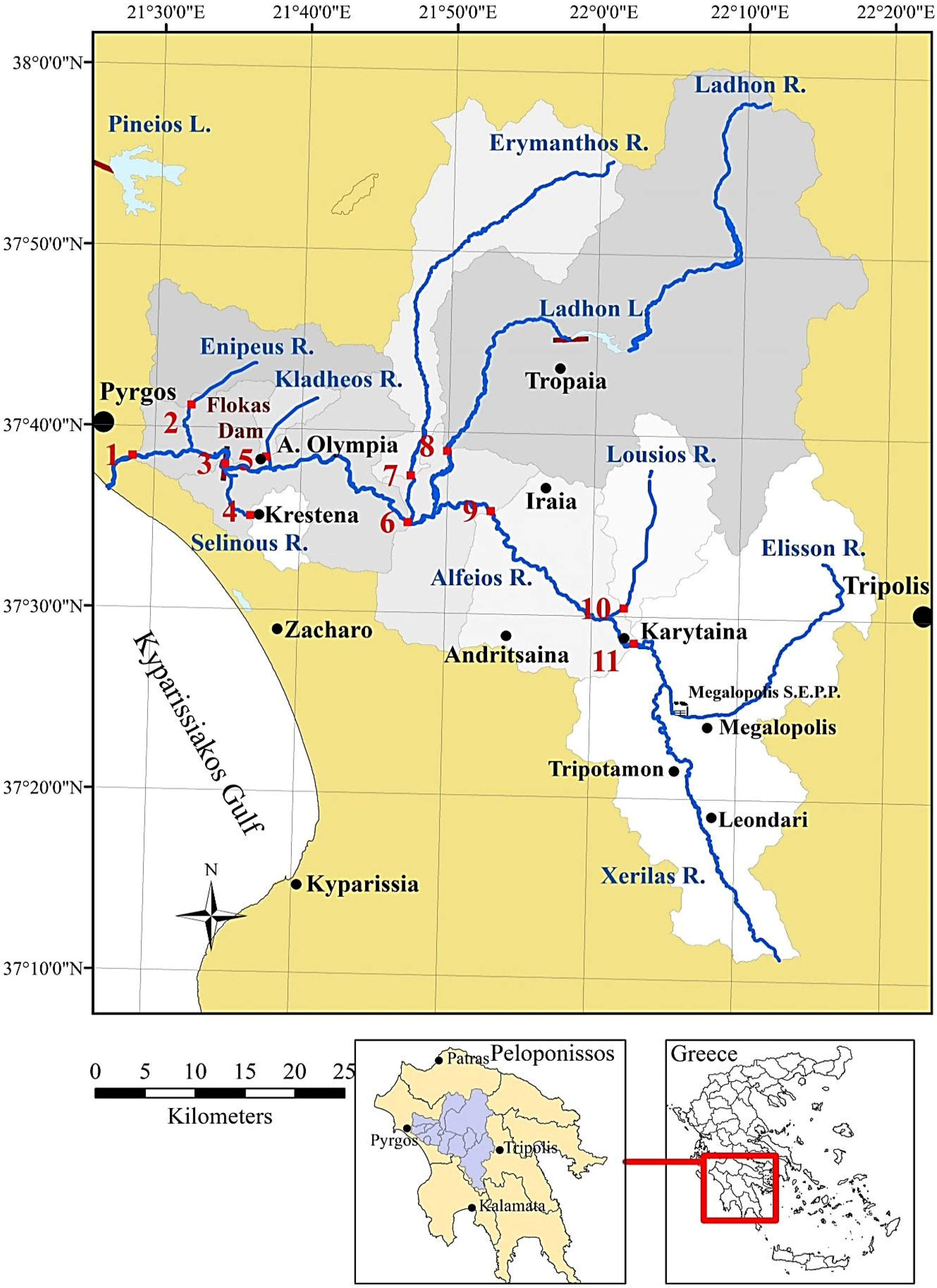

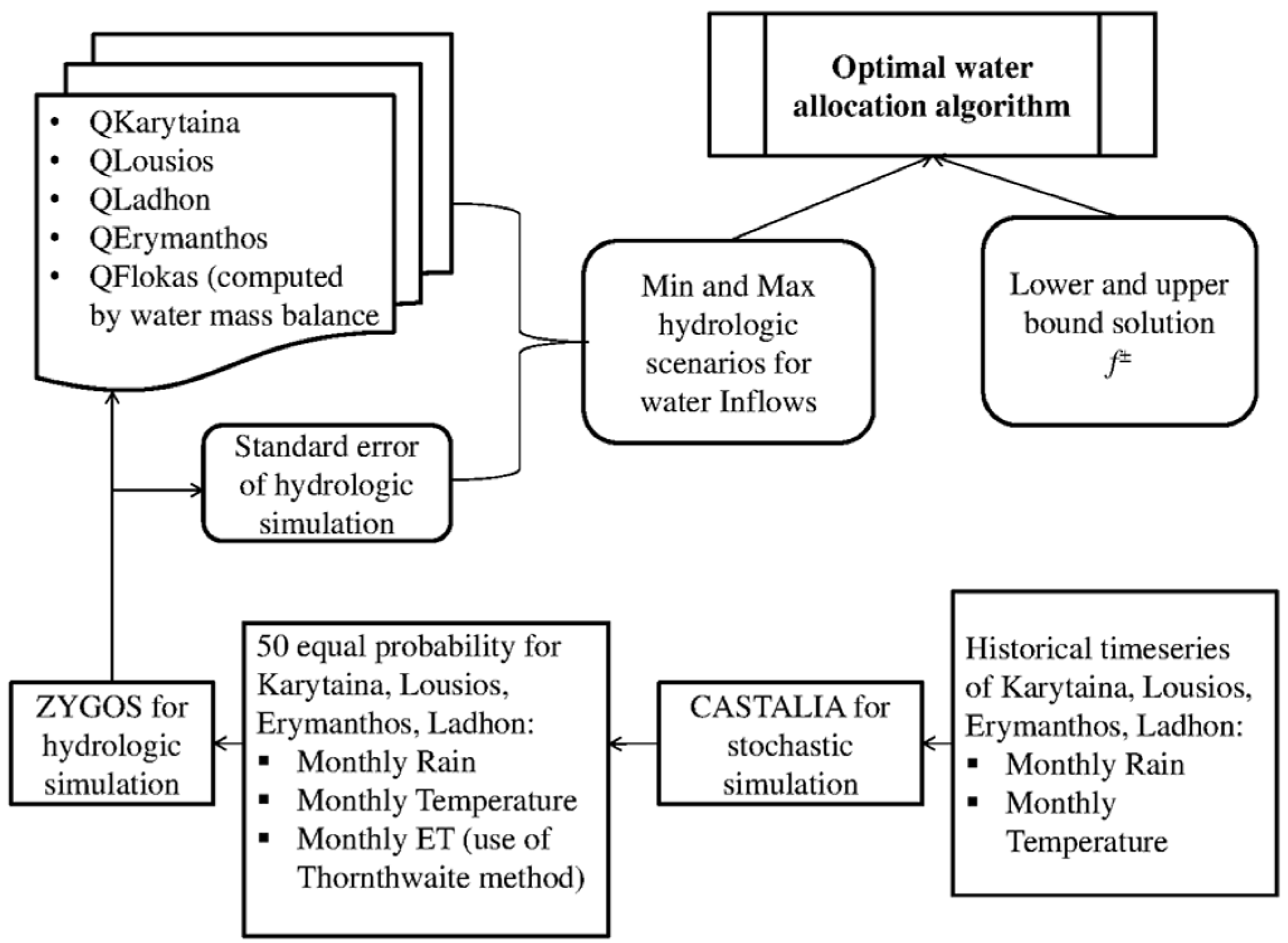