Empirical Formulas for Calculation of Negative Pressure Difference in Vacuum Pipelines

Abstract

The paper presents the analysis of results of empirical investigations of a negative pressure difference in vacuum pipelines with internal diameters of 57, 81, 102 mm. The investigations were performed in an experimental installation of a vacuum sewage system, built in a laboratory hall on a scale of 1:1. The paper contains a review of the literature concerning two-phase flows (liquid-gas) in horizontal, vertical and diagonal pipelines. It presents the construction and working principles of the experimental installation of vacuum sewage system in steady and unsteady conditions during a two-phase flow of water and air. It also presents a methodology for determination of formula for calculation of a negative pressure difference in vacuum pipelines. The results obtained from the measurements of the negative pressure difference Δp_vr in the vacuum pipelines were analyzed and compared with the results of calculations of the negative pressure difference Δp_vr, obtained from the determined formula. The values of the negative pressure difference Δp_vr calculated for the vacuum pipelines with internal diameters of 57, 81, and 102 mm with the use of Formula (19) coincide with the values of Δp_vr measured in the experimental installation of a vacuum sewage system. The dependence of the negative pressure difference Δp_vr along the length of the vacuum pipelines on the set negative pressure in the vacuum container p_vzp is linear. The smaller the vacuum pipeline diameter, the greater the negative pressure difference Δp_vr is along its length.

1. Introduction

The concept of a vacuum sewerage system began in documents in 1866, when a Dutchman, Charles Liernur patented this system with emptying valves for sanitary facilities. Despite the long history of the technical solution of collecting and transport of sewage to a neutralizing place, the literature on the topic is not voluminous. The first ideas of sewage disposal with the use of a pressure lower than the atmospheric pressure were abandoned for a long time after their birth. This was due to a lack of knowledge in the technical development of the time as well as the strong competition from gravitational sewage systems. Only in the 1950s, in Sweden, did the idea return. In this moment the development of modern vacuum sewerage systems began.

In the normative literature [1,2] concerning the construction and design of vacuum sewage systems, there is s lack of information on how to calculate a negative pressure difference in vacuum pipelines. Vacuum pipelines are pipelines where a reduced pressure occurs compared to the atmospheric pressure. The design requirements contained in directives are minimum requirements, which do not comprise full design directives sufficient to design a correctly operating system. The directives do not specify either a detailed range of a design or materials used to build components of the system. Information is given in the European standard [2] indicating that a vacuum sewage system should be individually designed with consideration of recommendations from suppliers of the devices for this system. The elaboration of the design recommendations, the exploitation rules and the range of application of the vacuum sewage system can be found in widely accessible scientific-technical literature [3,4,5,6,7,8,9,10,11].

Basing on the accessible scientific-technical literature, one can state that the hydraulic phenomena occurring during a flow of sewage-air mix in the vacuum sewage system are very weakly recognized. It appears from the performed investigations that they were carried out in single, short, straight and horizontal, vertical or diagonal pipelines and did not directly concern a complex vacuum sewage system [12,13,14,15,16,17,18,19,20]. The investigations were of general character and comprised two-phase (gas-liquid, liquid-solid or gas-solid) flows in stable hydraulic flow conditions. They were being carried out in pipelines with circular or rectangular sections. During these investigations the liquid flow and gas flow, in the majority of cases, were forced by force pumps, not vacuum pumps. It helped to recognize the flow structures in the liquid-gas medium flow in individual short horizontal, vertical or diagonal pipelines. So-called maps of two-phase (liquid-gas) flows were also worked out [12,21,22], but these maps do not have practical application to design vacuum sewage systems.

The investigations on determination of an equation for calculation of negative pressure difference in pipelines during two-phase (liquid-gas) flows [23,24,25] were also carried out. These investigations were also performed on single, short, straight and horizontal, vertical or diagonal sections of pipelines, with small diameters, without slopes (without a saw-type profile for the pipeline) occurring in the pipelines in vacuum sewage systems. Those equations were worked out on the basis of empirical investigations and statistical analysis and have restricted application. They can be applied only for the conditions corresponding to the range of variability of the parameters considered in the investigations. Polish researchers proposed to apply the results of those investigations to hydraulic calculations of pipelines transporting liquid-gas mix type sewages [26,27], but the range of their application in a vacuum sewage system is very restricted. The normative literature does not recommend to apply those equations to hydraulic calculations of pipelines in vacuum sewage systems [1,2].

Chenoweth and Martin [28], Hughmark [29,30] and Hughmark and Pressburg [31] carried out investigations on a pressure drop in vertical and horizontal pipelines during a two-phase flow of liquids and gases. The scope of their investigations encompassed not only water and air but also petroleum and air, gasoline and air, oil mixture and air, naphtha and air, gas oil and air, water and water foam, salt solutions and air. The investigations were carried out for various flow speeds of liquids and air. During these investigations, the liquid and air flow was forced by force pumps, not vacuum pumps.

Ratkovich et al. [20] investigated two-phase flows of gas and Newtonian liquid (air-water, air-pentanol, air-glycerin) as well as gas and non-Newtonian liquid (air and water solutions of sodium) in vertical pipes. The investigations encompassed three stages. The first one consisted in experimental tests of a two-phase flow with cork structure on a built measurement stand. The second stage encompassed simulation tests of a two-phase flow with a cork structure with use of a CFD (Computational Fluid Dynamic) model. The third stage encompassed a comparison of results of the simulation tests and results of the experimental tests as well as empirical formulas existing in the literature. The performed investigations showed that the CFD model can be successfully applied to predict two-phase flow with a cork structure in vertical pipes.

Cazarez-Candia et al. [18] worked out a one-dimensional mathematical model to simulate two-phase liquid-gas flows in pipelines applied to petroleum transport in oil wells. The authors carried out their investigations for cork flows of oil-water-gas mix. The mathematical model was built of the equations of principles of conservation of mass, momentum and energy, whereas the equations themselves were solved by FEM. The simulation tests of the two-phase flows were carried out in the pipelines with slope from 0° till 45° where an annular flow was assumed. It was investigated the influence of the temperature and compression-decompression processes of the gas on the stability of the constructed model. The results obtained from the simulation tests were compared to the results of experiments. It was stated that with use of the constructed mathematical model, 14% lower values were obtained than those from the performed experimental tests.

Irikura et al. [32] investigated the behavior of water in transparent V-shaped pipelines. The scope of their investigations encompassed pipes with diameters of 20, 30 and 40 mm and slope angles of 3°, 5° and 7°. The tests consisted in partially filling a pipe with water, then forcing air into it and observing how the water behaves via a given filling ratio of the pipe. At the beginning the water was at rest, and then it started to flow and formed a wave whose crest filled the whole section of the pipe. Then, as the beginning phase of the water flow was finished, the wave disappeared. The observed phenomenon of wave forming was described by the researchers as hydraulic strokes of the liquid resting in the V-shaped pipes. Based on the obtained results of the tests and after recognition of the wave forming phenomenon, the researchers worked out a three-dimensional mathematical model for simulations of hydraulic strokes of resting liquid in V-shaped pipes.

Skillman [33] who carried out investigations of flow of domestic sewages in a vacuum sewage system in separate pipelines with the diameters of 50, 75 and 100 mm, derived a dependence for a minimal capacity of a vacuum tank and determined a minimal transport velocity of the sewages as 1.05 m·s⁻¹. As the result of the several years’ investigations, he formulated 12 conclusions, and the most important of them are the following:

• The working effectiveness (including energy consuming) of the vacuum pipelines depends mainly on the ratio of the volume of introduced air to the volume of sewage (f), and to a lesser degree on the pipeline diameter and its configuration. The highest effectiveness was shown by the systems with relatively low ratio of f.
• Whirls in emptying wells can cause a 40% reduction of the velocity of sewage flow in pipelines. To avoid this, the well outlet should be placed in the sidewall of the well, not in the bottom.
• The required difference of pressures (negative pressure in the vacuum tank) should take into consideration the total height of elevation, not only the difference between elevations of the beginning and end of the pipeline (net height).
• Coefficients of linear resistance of two-phase mixtures flowing in vacuum pipelines cannot be determined from dependences for one-phase flows, though the latter can be a rough approximation of the former—the nearer to zero the phase volume ratio f is, the better.

However, Li et al. [34] proposed a two-dimensional hydrodynamic model for description of medium transport in vacuum sewage system pipelines, without its verification, on the basis of real hydraulic conditions of medium flow in a vacuum sewage system. The premises assumed in the model to describe the medium flow in the vacuum sewage system pipes were based on the investigations of Dukler and Hubbard [35] who, based on laboratory investigations in horizontal pipes, proposed a similar two-dimensional model for a description of transport of gas and liquid in horizontal pipes.

Attention must be paid to the item [36] concerning design principles of vacuum sewage systems. Bearing in mind the state of the scientific-technical knowledge in that time, one can state that the publication [36] played a pioneering role, because in 1983 no vacuum sewage systems were operated in Poland. However, from the point of view of current knowledge, it must be stated that many premises were assumed in this publication without any experimental grounds. Particularly, one false premise was assumed concerning a type of flow occurring in a saw-type profile vacuum collector.

In a vacuum sewage system, in steady and unsteady conditions, in separate sections of a vacuum pipeline, there occur very diverse structures of a liquid-gas mix flow [37,38]. The flow of liquid-gas mixture in a vacuum sewage system was investigated:

• in steady conditions without air sucking, i.e., during the tests the emptying valve was open all the time and the vacuum pipeline continuously sucked only water with a set flow rate;
• in steady conditions with air sucking, i.e., during the tests the emptying valve was open all the time and the vacuum pipeline continuously sucked water and air with a set flow rates;
• in unsteady conditions, i.e., during the tests the emptying valve was opened in random way (the opening time was set) and the vacuum pipeline sucked water first and then air.

The flow of a liquid-gas mix stream in the vacuum sewage system is very dynamic, unstable and pulsatory. The diversity of structures of medium flow in the vacuum sewage system is forced by the gravity force which aspires to stratify the phases. The diversity of structures of medium flow in the vacuum sewage system pipelines depends on a diameter, profile and height position of the pipeline in the system [37,38]:

• in steady conditions, without air suction, the following occur: bubbly flow, slug air flow, stratified air flow, annular flow, wave flow, air flow, slug flow, intermittent flow (projective);
• in steady conditions, with air suction, the following occur: projective flow, bubbly flow, slug flow, foam flow, wave flow, stratified flow, annular flow;
• in unsteady conditions, the following occur: foam flow, bubbly flow, projective flow (intermittent), slug air flow, stratified air flow, wave flow.

Multiphase flows occur not only in the pipelines of vacuum sewage systems but also, for example, in the pipelines applied for petroleum transport in oil wells, in the pipelines of air lifts, in water-pipe networks during a hydraulic stroke [39,40,41], in the pipelines of heat exchangers, in jet pumps, in pipelines transporting loose materials hydraulically, etc. The two-phase flows (liquid-gas) in the pipelines of air lifts are the best recognized. The investigations performed to date allowed to work out so-called flow structure maps for air lifts and mathematical models for simulations of the flows occurring there [42,43,44,45,46,47,48,49,50,51,52,53]. Investigations of air lifts made of rectangular [54] and crooked [55] pipes were also carried out. The tests performed on air lifts with crooked pipes beyond an air-water mixer show that the pumping capacity of solid bodies significantly falls in the air lifts constructed in such away. However, if only liquid is transported, then the pipe curvature of the air lift does not affect its capacity [56]. The performed investigations show that the air lifts are characterized by low operational efficiency compared to conventional pumps [45,46,57,58].

Multiphase flows occur most frequently in devices in the chemical and petrochemical industry, environmental engineering, in conventional and nuclear power engineering, and in heat engineering. The multiphase flows, however, which occur in the pipelines of technical devices cause a lot of design problems due to very diverse and unstable flow conditions.

Nowadays, during the design of vacuum sewage systems, hydraulic losses (pressure differences) in vacuum pipelines are not being taken into consideration because there is no formula for their calculation [1,2]. If an engineer does not know how to calculate the hydraulic losses (pressure differences) in vacuum pipelines, he/she is not able to select proper pumps for the vacuum sewage system, meaning the pumps chosen for such system are often characterized by improper operational parameters. In practice all users of the vacuum sewage systems complain that they operate improperly and are very energy-consuming. Due to this, there is an urgent necessity to determine a formula for calculation of the negative pressure difference in vacuum pipelines. This will help to make the design directives more precise.

On account of the very diverse hydraulic operating conditions of vacuum sewage systems [37,38] nobody in the world has yet worked out a mathematical model based on differential equations describing a way to calculate of the negative pressure difference along the length of the vacuum pipelines. As is known, if differential equations describing an investigated problem are not known, the dimensional analysis is applied as the first approach in such cases to solve the problem. By reason of this, the main aim of this paper is to present the analysis of results of investigations undertaken to solve this problem and to determine the formula for calculation of the negative pressure difference in vacuum pipelines by using dimensional analysis. The scope of the paper encompasses the derivation of the formula on the basis of empirical investigations performed on the constructed experimental installation of a vacuum sewage system for vacuum pipelines with internal diameters of 57, 81, and 102 mm.

2. Methodology of Derivation of Structural Equation

Taking into consideration that the structure types of air-water mix flow are so different and the operation of vacuum sewage systems is very dynamic and variable in time [9,10,37], it must be stated that the application of the classical mathematical model is currently impossible or at least very hard in order to work out a formula for calculation of difference of negative pressure in the pipelines of vacuum sewage systems. Due to this, dimensional analysis was applied to determine such a formula [59,60,61,62,63,64,65,66,67]. Basing on the performed investigations [37,38] it was assumed that the difference of negative pressure along the vacuum pipeline length depends on the following dimensional variables (Figure 1):

• Δp_vr—difference of negative pressure along the vacuum pipeline length, kg·m⁻¹·s⁻²;
• p_vzp—negative pressure in the vacuum container, kg·m⁻¹·s⁻²;
• d—vacuum pipeline internal diameter, m;
• L—vacuum pipeline length, m;
• Q_w—water flow rate, m³·s⁻¹;
• Q_p—air flow rate, m³·s⁻¹;
• ρ_w—water density, kg·m⁻³;
• ρ_p—air density, kg·m⁻³;
• μ_w—water dynamic viscosity, kg·m⁻¹·s⁻¹;
• μ_p—air dynamic viscosity, kg·m⁻¹·s⁻¹;
• g—gravitational acceleration, m·s⁻²;
• k—absolute roughness coefficient, m.

Figure 1. Calculation scheme for derivation of the structural equation.

Figure 1. Calculation scheme for derivation of the structural equation.

The vacuum pipelines in technical conditions are long (usually over 1 ÷ 2 km) and laid underground without warm insulation [2], so the temperature of gas (air) and liquid (sewage) is close to the ambient temperature. Thus it can be assumed that the gas and liquid temperature is constant along the pipeline length and the liquid and air flow is isothermal, i.e., $\frac{p}{{\mathrm{\rho }}_p}=const$, $\frac{p}{{{\displaystyle \mathrm{\rho }}}_w}=const$. The vacuum pipeline length L is a sum of lengths of ascending and descending sections which are measured along the axis of the vacuum pipeline (Figure 1). The negative pressure difference Δp_vr along the pipeline length is directly proportional to the pipeline length L. Taking the above assumptions into considerations, one can write out a dimensional equation describing the discussed phenomena:

$$f\left(\frac{{{\displaystyle \Delta p}}_{vr}}{L},\frac{{{\displaystyle p}}_{vzp}}{{{\displaystyle \mathrm{\rho }}}_w},\frac{{{\displaystyle p}}_{vzp}}{{{\displaystyle \mathrm{\rho }}}_p},{{\displaystyle \mathrm{\mu }}}_w,{{\displaystyle \mathrm{\mu }}}_p,d,{{\displaystyle Q}}_w,{{\displaystyle Q}}_p,g,k\right)=0$$

(1)

In this equation occurs n = 10 dimensional quantities, whose dimensions contain k = 3 basic units: m, kg, s. According to Buckingham’s II-theorem, this equation can be transformed into a connection of n − k = 7 mutually independent dimensionless parameters π. Three quantities were chosen—μ_w, d, Q_w—containing the given basic units and their dimensional independence was checked:

$${{\displaystyle [kg\cdot {{\displaystyle m}}^{-1}\cdot {{\displaystyle s}}^{-1}]}}^{{{\displaystyle a}}_1}\cdot {{\displaystyle [m]}}^{{{\displaystyle a}}_2}\cdot {{\displaystyle [{{\displaystyle m}}^3\cdot {{\displaystyle s}}^{-1}]}}^{{{\displaystyle a}}_3}=b$$

$${{\displaystyle kg}}^{{{\displaystyle a}}_1}\cdot {{\displaystyle m}}^{{{\displaystyle -a}}_1}\cdot {{\displaystyle s}}^{{{\displaystyle -a}}_1}\cdot {{\displaystyle m}}^{{{\displaystyle a}}_2}\cdot {{\displaystyle m}}^{{{\displaystyle 3a}}_3}\cdot {{\displaystyle s}}^{{{\displaystyle -a}}_3}=b$$

$${{\displaystyle m}}^{{{\displaystyle -a}}_1+{{\displaystyle a}}_2+{{\displaystyle 3a}}_3}\cdot {{\displaystyle kg}}^{{{\displaystyle a}}_1}\cdot {{\displaystyle s}}^{{{\displaystyle -a}}_1-{{\displaystyle a}}_3}={{\displaystyle [m]}}^0\cdot {{\displaystyle [kg]}}^0{{\displaystyle [s]}}^0$$

$$\begin{array}{r}\hfill {{\displaystyle -a}}_1+{{\displaystyle a}}_2+{{\displaystyle 3a}}_3=0\Rightarrow {{\displaystyle a}}_2=0\\ \hfill {{\displaystyle a}}_1=0\Rightarrow {{\displaystyle a}}_1=0\\ \hfill {{\displaystyle -a}}_1-{{\displaystyle a}}_3=0\Rightarrow {{\displaystyle a}}_3=0\end{array}$$

Hence a₁ = a₂ = a₃ = 0, b = 1 (they are dimensionally independent).

A consecutive connection of the remaining quantities with the product of powers of the chosen dimensionally independent quantities allowed us to determine the dimensionless parameters π:

$${{\displaystyle \mathrm{\pi }}}_1=\frac{{{\displaystyle \Delta p}}_{vr}}{L}{{\displaystyle \mathrm{\mu }}}_w^{{{\displaystyle a}}_1}{{\displaystyle d}}^{{{\displaystyle a}}_2}{{\displaystyle Q}}_w^{{{\displaystyle a}}_3}$$

(2)

$${{\displaystyle \mathrm{\pi }}}_2=\frac{{{\displaystyle p}}_{vzp}}{{{\displaystyle \mathrm{\rho }}}_w}{{\displaystyle \mathrm{\mu }}}_w^{{{\displaystyle b}}_1}{{\displaystyle d}}^{{{\displaystyle b}}_1}{{\displaystyle Q}}_w^{{{\displaystyle b}}_3}$$

(3)

$${{\displaystyle \mathrm{\pi }}}_3=\frac{{{\displaystyle p}}_{vzp}}{{{\displaystyle \mathrm{\rho }}}_p}{{\displaystyle \mathrm{\mu }}}_w^{{{\displaystyle c}}_1}{{\displaystyle d}}^{{{\displaystyle c}}_1}{{\displaystyle Q}}_w^{{{\displaystyle c}}_3}$$

(4)

$${{\displaystyle \mathrm{\pi }}}_4={{\displaystyle \mathrm{\mu }}}_p{{\displaystyle \mathrm{\mu }}}_w^{{{\displaystyle d}}_1}{{\displaystyle d}}^{{{\displaystyle d}}_1}{{\displaystyle Q}}_w^{{{\displaystyle d}}_3}$$

(5)

$${{\displaystyle \mathrm{\pi }}}_5={{\displaystyle Q}}_p{{\displaystyle \mathrm{\mu }}}_w^{{{\displaystyle e}}_1}{{\displaystyle d}}^{{{\displaystyle e}}_1}{{\displaystyle Q}}_w^{{{\displaystyle e}}_3}$$

(6)

$${{\displaystyle \mathrm{\pi }}}_6=g{{\displaystyle \mathrm{\mu }}}_w^{{{\displaystyle f}}_1}{{\displaystyle d}}^{{{\displaystyle f}}_1}{{\displaystyle Q}}_w^{{{\displaystyle f}}_3}$$

(7)

$${{\displaystyle \mathrm{\pi }}}_7=k{{\displaystyle \mathrm{\mu }}}_w^{{{\displaystyle g}}_1}{{\displaystyle d}}^{{{\displaystyle g}}_1}{{\displaystyle Q}}_w^{{{\displaystyle g}}_3}$$

(8)

A substitution of the dimensions of the individual quantities and comparison of the power exponents in the basic units of the both sides of consecutive equations (analogically as during checking of the dimensional independence of the quantities) enables us to determine the values of the parameters π:

$${{\displaystyle \mathrm{\pi }}}_1=\frac{{{\displaystyle \Delta p}}_{vr}{{\displaystyle d}}^4}{L{{\displaystyle \mathrm{\mu }}}_w{{\displaystyle Q}}_w}$$

(9)

$${{\displaystyle \mathrm{\pi }}}_2=\frac{{{\displaystyle p}}_{vzp}{{\displaystyle d}}^4}{{{\displaystyle \mathrm{\rho }}}_w{{\displaystyle Q}}_w^2}$$

(10)

$${{\displaystyle \mathrm{\pi }}}_3=\frac{{{\displaystyle p}}_{vzp}{{\displaystyle d}}^4}{{{\displaystyle \mathrm{\rho }}}_p{{\displaystyle Q}}_w^2}$$

(11)

$${{\displaystyle \mathrm{\pi }}}_4=\frac{{{\displaystyle \mathrm{\mu }}}_p}{{{\displaystyle \mathrm{\mu }}}_w}$$

(12)

$${{\displaystyle \mathrm{\pi }}}_5=\frac{{{\displaystyle Q}}_p}{{{\displaystyle Q}}_w}$$

(13)

$${{\displaystyle \mathrm{\pi }}}_6=\frac{g{{\displaystyle d}}^5}{{{\displaystyle Q}}_w^2}$$

(14)

$${{\displaystyle \mathrm{\pi }}}_7=\frac{k}{d}$$

(15)

According to the Buckingham’s theorem, the dimensional Equation (1) can be written in the form of a dimensionless dependence of the parameters π:

$$f({{\displaystyle \mathrm{\pi }}}_1,{{\displaystyle \mathrm{\pi }}}_2,{{\displaystyle \mathrm{\pi }}}_3,{{\displaystyle \mathrm{\pi }}}_4,{{\displaystyle \mathrm{\pi }}}_5,{{\displaystyle \mathrm{\pi }}}_6,{{\displaystyle \mathrm{\pi }}}_7)=0$$

(16)

hence

$${{\displaystyle \mathrm{\pi }}}_1=f({{\displaystyle \mathrm{\pi }}}_2,{{\displaystyle \mathrm{\pi }}}_3,{{\displaystyle \mathrm{\pi }}}_4,{{\displaystyle \mathrm{\pi }}}_5,{{\displaystyle \mathrm{\pi }}}_6,{{\displaystyle \mathrm{\pi }}}_7)$$

(17)

A replacement of the values of π with the terms (9–15) and a rearrangement yields the structural equation:

$${{\displaystyle \Delta p}}_{vr}=f\left(\frac{{{\displaystyle p}}_{vzp}{{\displaystyle d}}^4}{{{\displaystyle \mathrm{\rho }}}_w{{\displaystyle Q}}_w^2},\frac{{{\displaystyle p}}_{vzp}{{\displaystyle d}}^4}{{{\displaystyle \mathrm{\rho }}}_p{{\displaystyle Q}}_w^2},\frac{{{\displaystyle \mathrm{\mu }}}_p}{{{\displaystyle \mathrm{\mu }}}_w},\frac{{{\displaystyle Q}}_p}{{{\displaystyle Q}}_w},\frac{g{{\displaystyle d}}^5}{{{\displaystyle Q}}_w^2},\frac{k}{d}\right)\frac{L{{\displaystyle \mathrm{\mu }}}_w{{\displaystyle Q}}_w}{{{\displaystyle d}}^4}$$

(18)

After the derivation of the structural Equation (18), the experiment was carried out in order to determine numerical coefficients for this equation in steady operating conditions of the experimental installation of a vacuum sewage system.

The dimensional variables in the Equation (18):

• ρ_w, μ_w—determine the physical properties of water,
• ρ_p, μ_p—determine the physical properties of air;
• d, k, L—characterize the object of the investigations, i.e., the vacuum pipelines—these quantities are constant;
• p_vzp, Q_w, Q_p—determine so-called input parameters, enabling the intentional action on the object of the investigations—these quantities are controllable and under control;
• Δ_pvr—determines so-called output parameter—it is the response of the object of the investigations to the input parameters.

The dimensionless variables in the Equation (18):

• π₁—determines the quotient of the forces evoked by the negative pressure difference to the friction forces;
• π₂ and π₃—determines the quotient of the forces evoked by the negative pressure to the dynamic forces;
• π₄—determines the quotient of the air friction (viscosity) forces to the water friction (viscosity) forces;
• π₅—determines the quotient of the air flow to the water flow;
• π₆—determines the quotient of the gravity forces to the dynamic forces evoked by the water flow;
• π₇—determines the relative roughness of the internal surface of the pipeline.

3. Experimental Procedures

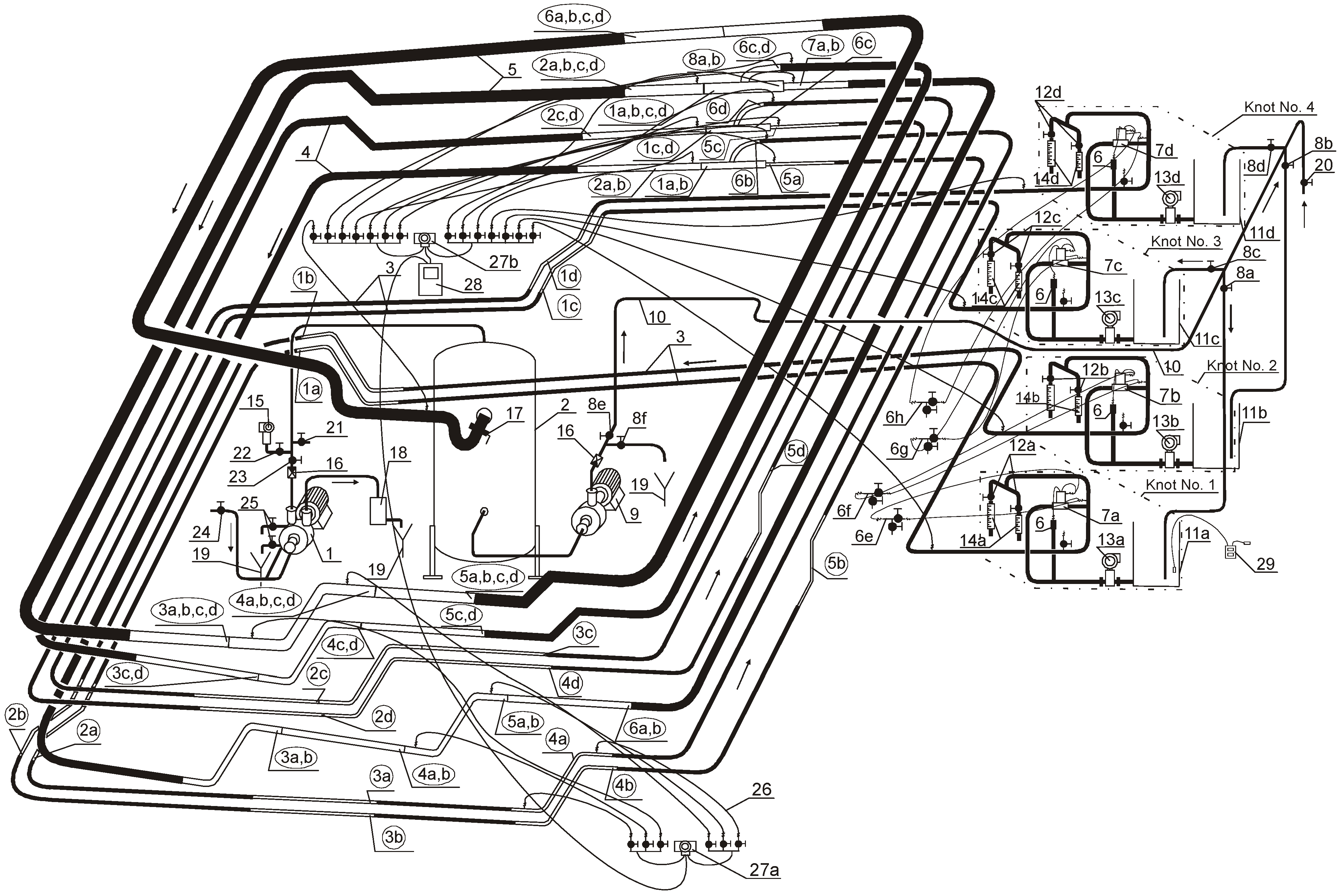
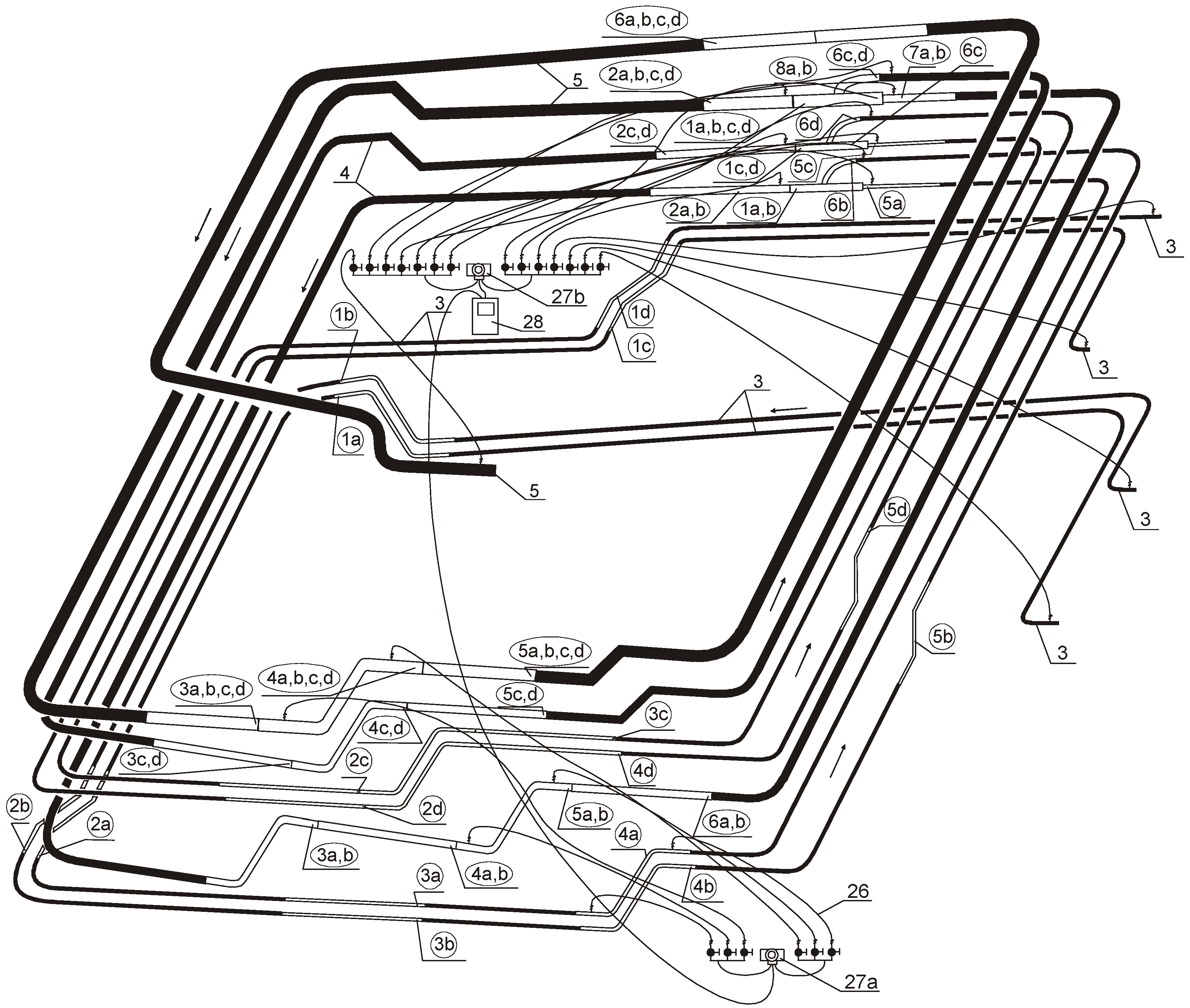
3.1. Description of Experimental Installation of Vacuum Sewage System

The experimental installation of a vacuum sewage system was built in a laboratory hall at a scale of 1:1 (Figure 2), within the context of research project WULS No. 50405250012 “Experimental researches of hydraulic flow conditions in collectors of vacuum sewage system” [38], funded from Scientific Research Committee resources. To build the experimental installation of a vacuum sewage system, typical materials and devices were used, being applied to build sewage systems of that type. There were used four ROEVAC type emptying knots, mounted at various heights. Two emptying knots were installed on the hall floor level and two at the height of 2.0 m over the floor, on scaffolding made of montage rails. As it is recommended that vacuum sewage systems be built on flat terrain, the difference between the pipelines height levels in the experimental installation was small, at 3.0 m [1,2]. The vacuum pipelines of the experimental installation of vacuum sewage system were mounted on appropriately prepared scaffolding made of montage rails. The total length of all vacuum pipeline arms was equal:

• for an internal diameter of 57 mm–96 m;
• for an internal diameter of 81 mm–44 m;
• for an internal diameter of 102 mm–42 m.

At the pipelines with an internal diameter of 57 mm (3) twelve slopes with a height of 0.30 m were applied, at the pipelines with an internal diameter of 81 mm (4)—five slopes with the height of 0.40 m, and at the pipelines with the internal diameter of 102 mm (5)—three slopes with the height of 0.35 m. The number of slopes at the individual vacuum pipelines depends on the height of their position in the experimental installation of a vacuum sewage system.

Figure 2 shows the scheme of the experimental installation of vacuum sewage system. However, Figure 3, Figure 4 and Figure 5 present the main elements that the constructed experimental installation of vacuum sewage system (Figure 2) consists of. The observation stands 1a ÷ 6a,b,c,d were made of transparent PMMA pipes and the remaining net was made of PVC pipes. The transparent sections of the vacuum pipes served to recognize types of medium flow occurring in various conditions as well as to visualize them. The transparent container (18), however, prevented from spoiling water at the laboratory hall when the vacuum pump was being started as well to supervise its function. The applied vacuum container (2) had a capacity of 2.5 m³. The mediums transported in the experimental installation were water and air. The installation was able to work both in a closed system and in the open one as well as under the conditions of steady and unsteady motion.

Figure 2. Scheme of the experimental installation of vacuum sewage system: 1-vacuum pump; 2-vacuum container; 3-vacuum pipeline with diameter of 57 mm; 4-vacuum pipeline with diameter of 81 mm; 5-vacuum pipeline with diameter of 102 mm; 6-sensor pipe; 6e,f,g,h-cutoff valve; 7a,b,c,d-interface valve; 8a,b,c,d,e,f-control valve; 9-water pump; 10-pressure pipeline; 11a,b,c,d-collector well; 12a,b,c,d-air control valve; 13a,b,c,d-electronic liquid flow meter; 14a,b,c,d-rotameter; 15-eelectronic meter of absolute pressure; 16-non-return valve; 17-throttling valve; 18-transparent container; 19-sewerage drain; 20-liquid supplying system cut-off valve; 21-vacuum container negative pressure control valve; 22, 23-vacuum pump air cut-off valve; 24-vacuum pump water cut-off valve; 25-vacuum pump working control valve; 26-impulse hose, 1a-6d-stand for observation of flow structures; 27a,b-electronic meter of pres-sure difference; 28-register of measurement results; 29-electronic termometer.

Figure 2. Scheme of the experimental installation of vacuum sewage system: 1-vacuum pump; 2-vacuum container; 3-vacuum pipeline with diameter of 57 mm; 4-vacuum pipeline with diameter of 81 mm; 5-vacuum pipeline with diameter of 102 mm; 6-sensor pipe; 6e,f,g,h-cutoff valve; 7a,b,c,d-interface valve; 8a,b,c,d,e,f-control valve; 9-water pump; 10-pressure pipeline; 11a,b,c,d-collector well; 12a,b,c,d-air control valve; 13a,b,c,d-electronic liquid flow meter; 14a,b,c,d-rotameter; 15-eelectronic meter of absolute pressure; 16-non-return valve; 17-throttling valve; 18-transparent container; 19-sewerage drain; 20-liquid supplying system cut-off valve; 21-vacuum container negative pressure control valve; 22, 23-vacuum pump air cut-off valve; 24-vacuum pump water cut-off valve; 25-vacuum pump working control valve; 26-impulse hose, 1a-6d-stand for observation of flow structures; 27a,b-electronic meter of pres-sure difference; 28-register of measurement results; 29-electronic termometer.

The operating principle of the experimental installation of a vacuum sewage system (Figure 2) in unsteady flow conditions was following: After the throttling valve (17) had been opened and the vacuum pump (1) had been started, a negative pressure arose in the vacuum container (2) and vacuum pipelines system (3)–(5). When it reached an appropriate value, which was read at the electronic meter of absolute pressure (15), the water pump (9) was started and pressed water from the vacuum container (2) through the pressure pipeline (10) to appropriate collector wells (11a,b,c,d). Then the control valve (8f) was closed and the control valve (8e) as well as appropriate control valves (8a,b,c,d) were opened. The emptying valves were opened automatically in a random way, depending on each collector well being filled with water. When an appropriate collector well (11a,b,c,d) was filled with water, the appropriate pressure arose in the sensor pipe (6) and was passed through the impulse hose to the pneumatic controller, then the interface valve (7a,b,c,d) was opened and the water from the collector well was sucked into the vacuum pipeline net. After the water had been sucked out from the collector well, the emptying valve stayed opened for a couple of seconds, and in this time the air was sucked into the experimental installation. After the air had been sucked into the vacuum pipeline net, the barometric pressure arose in the sensor pipe (6) and was passed through the impulse hose to the pneumatic controller, and then the interface valve (7a,b,c,d) was closed.

Figure 3. Emptying knots acc. Figure 2: 3-vacuum pipeline with diameter of 57 mm; 6-sensor pipe; 6e,f,g,h-cutoff valve; 7a,b,c,d-interface valve; 8a,b,c,d-control valve; 10-pressure pipeline; 11a,b,c,d-collector well; 12a,b,c,d-air control valve; 13a,b,c,d-electronic liquid flow meter; 14a,b,c,d-rotameter; 20-liquid supplying system cut-off valve; 29-electronic thermometer.

Figure 3. Emptying knots acc. Figure 2: 3-vacuum pipeline with diameter of 57 mm; 6-sensor pipe; 6e,f,g,h-cutoff valve; 7a,b,c,d-interface valve; 8a,b,c,d-control valve; 10-pressure pipeline; 11a,b,c,d-collector well; 12a,b,c,d-air control valve; 13a,b,c,d-electronic liquid flow meter; 14a,b,c,d-rotameter; 20-liquid supplying system cut-off valve; 29-electronic thermometer.

In steady flow conditions, however, the working principle of the experimental installation of vacuum sewage system (Figure 2) was the following: After the throttling valve (17) had been opened and the vacuum pump (1) had been started, a negative pressure arose in the vacuum container (2) and vacuum pipelines system (3–5). When it reached an appropriate value which was read at the electronic meter of absolute pressure (15), the appropriate interface valves (7a,b,c,d) were started with help of the cut-off valves (6e,f,g,h) at the distributor. Then the control valve (8f) was closed and the control valve (8e) as well as appropriate control valves (8a,b,c,d) were opened. The water pump (9) was started and pressed water from the vacuum container through the pressure conduit (10) to appropriate collector wells (11a,b,c,d). The air was led into the experimental installation through the rotameters (14a,b,c,d) by opening the appropriate air control valves (12a,b,c,d).

Figure 4. Vacuum pipelines acc. Figure 2: 3-vacuum pipeline with diameter of 57 mm; 4-vacuum pipeline with diameter of 81 mm; 5-vacuum pipeline with diameter of 102 mm; 26-impulse hose, 1a-6d-stand for observation of flow structures; 27a,b-electronic meter of pres-sure difference; 28-register of measurement results.

Figure 4. Vacuum pipelines acc. Figure 2: 3-vacuum pipeline with diameter of 57 mm; 4-vacuum pipeline with diameter of 81 mm; 5-vacuum pipeline with diameter of 102 mm; 26-impulse hose, 1a-6d-stand for observation of flow structures; 27a,b-electronic meter of pres-sure difference; 28-register of measurement results.

Figure 5. Vacuum station acc. Figure 2: 1-vacuum pump; 2-vacuum container; 5-vacuum pipeline with diameter of 102 mm; 8e,f-control valve; 9-water pump; 10-pressure pipeline; 15-eelectronic meter of absolute pressure; 16-non-return valve; 17-throttling valve; 18-transparent container; 19-sewerage drain; 21-vacuum container negative pressure control valve; 22, 23-vacuum pump air cut-off valve; 24-vacuum pump water cut-off valve; 25-vacuum pump working control valve.

Figure 5. Vacuum station acc. Figure 2: 1-vacuum pump; 2-vacuum container; 5-vacuum pipeline with diameter of 102 mm; 8e,f-control valve; 9-water pump; 10-pressure pipeline; 15-eelectronic meter of absolute pressure; 16-non-return valve; 17-throttling valve; 18-transparent container; 19-sewerage drain; 21-vacuum container negative pressure control valve; 22, 23-vacuum pump air cut-off valve; 24-vacuum pump water cut-off valve; 25-vacuum pump working control valve.

3.2. Methodology of Measurements

When the changes and difference in the negative pressure along the length of the vacuum pipelines had been recognized in unsteady conditions, it turned out that the maximum and minimum values of these changes are fairly stable [37,38]. The dependence of the negative pressure and its difference along the length of the vacuum pipelines on the negative pressure in the vacuum container is linear. From the point of view of the design principles, the maximum changes of the negative pressure difference (the emptying valve opening) are more important. The difference of the negative pressure drop in long sections of vacuum pipelines in dependence on the negative pressure changes in a vacuum container is small and fairly stable.

Due to this, an experiment was performed on the experimental installation of a vacuum sewage system (Figure 2) in order to determine a numerical coefficient for structural Equation (18) in steady conditions of operation for the experimental installation.

The investigations of changes of the negative pressure differences Δp_vr along the length of the vacuum pipelines in steady conditions for the set absolute pressures p_zp in the vacuum container and the air flow rate Q_p were performed between the measuring points: 1a and 4a for the internal diameter of 57 mm, 5a and 8b for the internal diameter of 81 mm, 9abcd and 11abcd for the internal diameter of 102 mm (Figure 6), when one emptying knot—No. 1 (Figure 2)—was operating.

Figure 6. Expansion of the experimental installation of vacuum sewerage acc. Figure 2: 1a, …, 11abcd—measuring points on the vacuum pipeline; Wo1, …, Wo4—emptying knot; Zp—vacuum container; a, …, abcd—vacuum pipelines; d = 57 mm—vacuum pipeline internal diameter.

Figure 6. Expansion of the experimental installation of vacuum sewerage acc. Figure 2: 1a, …, 11abcd—measuring points on the vacuum pipeline; Wo1, …, Wo4—emptying knot; Zp—vacuum container; a, …, abcd—vacuum pipelines; d = 57 mm—vacuum pipeline internal diameter.

Before starting each measuring series (Figure 2) and after starting the measuring devices, current barometric pressure p_b was read. When this actual barometric pressure p_b during the measuring series and the absolute pressure p_zp in the vacuum container were known, the negative pressure p_vzp in the vacuum container was calculated. One of the ends of the electronic thermometer (29) was placed in the collector well (11a) in order to measure the current temperature T_w of the liquid (water) supplied to the system, and the other end was led outside to measure the current temperature T_p of the air supplied to the system. The set absolute pressure p_zp in the vacuum container and the set air flow rate Q_p were maintained during the investigations.

When the experimental installation of vacuum sewage system (Figure 2) had been started, the first value of the absolute pressure (p_zp = 20 kPa) in the vacuum container was set with the valve (21) and, with use of the electronic meter of absolute pressure (15), we monitored whether the value of the absolute pressure remains constant in the vacuum container. Then the first value of the air flow rate (Q_p = 4 m³·h⁻¹) was set on the rotameter (14a) with the valve (12a) and, after stabilization of the hydraulic flow conditions in the system, the following quantities were read: on the electronic thermometer (29)—the temperature T_w of the supplied liquid (water) and the temperature T_p of the supplied gas (air); on the electronic liquid flow meter (13a)—the water flow rate Q_w for the set air flow rate Q_p; on the electronic meter of negative pressure difference, for every pipeline diameter (switching appropriately with the cut-off valves (27b) at the distributor)—the negative pressure difference Δp_vr along the length of a given pipeline.

Then the subsequent values of the absolute pressure p_zp (25 kPa, 30 kPa, 35 kPa, 40 kPa, 45 kPa) in the vacuum container were set for a constant value of the air flow rate (Q_p = 4 m³·h⁻¹) and after stabilization of the hydraulic flow conditions in the system, the readings of each measuring devices were read.

When a measuring series was finished, the system operation was stopped. The next measuring series was started for the next set value of the air flow rate (Q_p = 8 m³·h⁻¹) after the system depressurization. The measurements were carried out for the set values of the absolute pressure in the vacuum container p_zp from 20 to 45 kPa with step 5 kPa and for the set values of the air flow rate Q_p from 4 to 40 m³·h⁻¹ with step 4 m³·h⁻¹. For each pipeline diameter as well as for each set value of the air flow rate and the absolute pressure in the vacuum container, nine measuring series were performed.

The level difference between the measuring points of the negative pressure difference Δp_vr for each pipeline diameter was also measured. Then the measured values of the negative pressure difference Δp_vr were corrected with the level difference between the measuring points of the Δp_vr. This allowed us to obtain a real difference of the negative pressure Δp_vr along the pipeline length, resulting only from the existing hydraulic resistance during the air-liquid mix flow.

4. Results and Discussion

Using the results of the measurements performed in the built experimental installation of vacuum sewage system (Figure 2) for steady flow conditions, the dimensionless parameters: π₁ (9), π₂ (10), π₃ (11), π₄ (12), π₅ (13), π₆ (14), π₇ (15) were calculated from the determined structural Equation (18). Depending on the measured temperature of liquid T_w and air T_p, based on the tables [68], the following quantities were determined: water density ρ_w, air density ρ_p, water dynamic viscosity μ_w, air dynamic viscosity μ_p. Then, appropriate data sheets were constructed and, with use of the multiple regression method and the computer program STATISTICA [69], for the internal diameters of 57, 81, and 102 mm, the numerical coefficients were determined for the formula. In order to determine slopes of the straight lines, the additive model of the multiple regression was assumed, because the performed investigations [37,38] showed that the change of the negative pressure difference Δp_vr is of a linear character. The additive model can be applied exactly in the case if a trend function is linear or allows to transfer to linear function.

After substitution of the determined numerical coefficients to the structural Equation (18) and after reduction of the significant digits on account of simplifications in formula application, finally the formula for calculation of the negative pressure difference Δp_vr in vacuum pipelines with internal diameters of 57, 81, and 102 mm for the range $\frac{{{\displaystyle Q}}_p}{{{\displaystyle Q}}_w}=0.26÷8.4$ was determined:

$${{\displaystyle \Delta p}}_{vr}=\left(12100-19.33\frac{{{\displaystyle p}}_{vzp}{{\displaystyle d}}^4}{{{\displaystyle \mathrm{\rho }}}_w{{\displaystyle Q}}_w^2}+0.022\frac{{{\displaystyle p}}_{vzp}{{\displaystyle d}}^4}{{{\displaystyle \mathrm{\rho }}}_p{{\displaystyle Q}}_w^2}-85300\frac{{{\displaystyle \mathrm{\mu }}}_p}{{{\displaystyle \mathrm{\mu }}}_w}+380\frac{{{\displaystyle Q}}_p}{{{\displaystyle Q}}_w}-45\frac{g{{\displaystyle d}}^5}{{{\displaystyle Q}}_w^2}-23518000\frac{k}{d}\right)\frac{L{{\displaystyle \mathrm{\mu }}}_w{{\displaystyle Q}}_w}{{{\displaystyle d}}^4}$$

(19)

where,

• Δp_vr—negative pressure difference in pipeline, Pa;
• p_vzp—negative pressure in vacuum container, kg·m⁻¹·s⁻²;
• d—pipeline internal diameter, m;
• L—pipeline length, m;
• Q_w—water flow rate, m³·s⁻¹;
• Q_p—air flow rate, m³·s⁻¹;
• ρ_w—water density, kg·m⁻³;
• ρ_p—air density, kg·m⁻³;
• μ_w—water dynamic viscosity, kg·m⁻¹·s⁻¹;
• μ_p—air dynamic viscosity, kg·m⁻¹·s⁻¹;
• g—gravitational acceleration, m·s⁻²;
• k—absolute roughness coefficient, m.

The range $\frac{{{\displaystyle Q}}_p}{{{\displaystyle Q}}_w}$ was calculated according to the performed measurements in the experimental installation of a vacuum sewage system (Figure 2). The lower limit of the range was calculated for the negative pressure in the vacuum container p_vzp = 81 kPa for the set air flow rate Q_p = 4 m³·h⁻¹ and the upper limit of the range was calculated for the negative pressure in the vacuum container p_vzp = 55 kPa for the set air flow rate Q_p = 40 m³·h⁻¹.

Figure 7 shows the results of measurements of the negative pressure difference Δp_vr and its calculations with use of the Formula (19) determined for the pipelines with internal diameters of 57, 81, and 102 mm. The functional dependence between the negative pressure difference Δp_vr and the vacuum container pressure p_vzp is of linear character both for the values obtained from the measurements and from the calculations with the use of the determined Formula (19). Deviations between the values of Δp_vr obtained from the calculations and the values of Δp_vr obtained from the measurements are small for the pipelines with the internal diameter of 57, 81 and 102 mm. The regression type is linear for the values of the negative pressure difference Δp_vr obtained from the calculations with use of the determined formula as well as for the values of Δp_vr obtained from the measurements. The trend lines for the negative pressure difference Δp_vr obtained from the calculations are slightly moved compared to the trend lines for the values of Δp_vr obtained from the measurements.

In steady conditions of system operation, the distance between the trend lines (along Y axis) for the pipelines with the internal diameters of 81 and 102 mm is small if compared with the distances between the trend lines for these two pipelines and for the pipeline with the diameter of 57 mm. This relation meets the expectations because, in the pipes with small diameters, the negative pressure differences Δp_vr along the pipe length are greater than in the pipes with large diameters transporting the same quantity of sewage. In the vacuum pipelines with small diameters, the slopes are closed with liquid, and in those with large diameters they are not, so in the pipelines with large diameters the negative pressure along their length is more leveled.

Figure 7. Functional dependence between the negative pressure difference (Δp_vr) and the vacuum container pressure (p_vzp) for the data calculated from the empirical formula and for the measured data.

Figure 7. Functional dependence between the negative pressure difference (Δp_vr) and the vacuum container pressure (p_vzp) for the data calculated from the empirical formula and for the measured data.

To evaluate the accuracy of the calculation results from Formula (19), the values Δp_vr calculated from Formula (19) were compared to the values Δp_vr measured in the experimental installation of vacuum sewage system. It was stated that for the parameters:

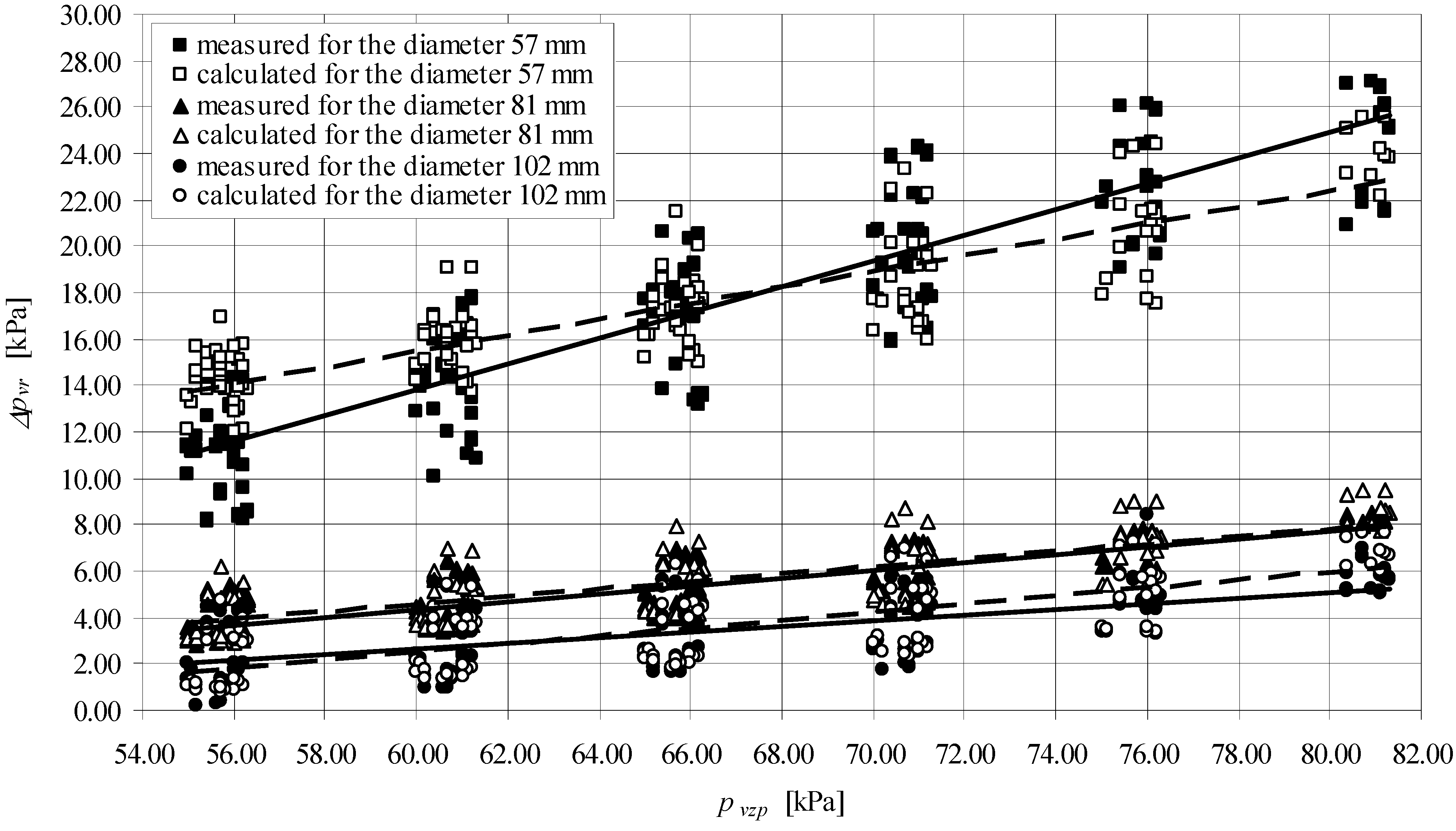
• d = 0.057 m; d = 0.081 m; d = 0.102 m;
• 55 kPa < p_vzp < 81 kPa;
• 4.80 m³·h⁻¹ < Q_w < 15.40 m³·h⁻¹;
• 4.00 m³·h⁻¹ < Q_p < 40.00 m³·h⁻¹;
• 1.2046 kg·m⁻³ < ρ_p < 1.2154 kg·m⁻³;
• 998.2478 kg·m⁻³ < ρ_w < 998.5148 kg·m⁻³;
• 1.0113·10⁻³ kg·m⁻¹·s⁻¹ < μ_w < 1.0788·10⁻³ kg·m⁻¹·s⁻¹;
• 1.7970·10⁻⁵ kg·m⁻¹·s⁻¹ < μ_p < 1.8150·10⁻⁵ kg·m⁻¹·s⁻¹;

the average deviation of Δp_vr does not exceed 18% for the pipeline with an internal diameter of 57 mm, 9% for 81 mm, and 20% for 102 mm (Figure 7).

Moreover, an analysis of the left and right side of the Formula (19) was performed and it showed that the dimensions of both sides of the formula agree with each other.

5. Conclusions

The changes of the negative pressure difference Δp_vr along the length of the vacuum pipelines in dependence on the set negative pressure p_vzp in the vacuum container are linear. The smaller the vacuum pipeline diameter is, the greater the negative pressure difference Δp_vr along the pipeline length. The dispersion of the measured values of Δp_vr is greater if the pipeline internal diameter is smaller. This means that the bigger the pipeline internal diameter is, the more stable the flow conditions of the medium are.

The values of the negative pressure difference Δp_vr calculated for the vacuum pipelines with diameters of 57, 81, and 102 mm with the use of Formula (19) coincide with the values of Δp_vr measured in the experimental installation of a vacuum sewage system. Bearing in mind that the operating conditions of the vacuum sewage system are so very dynamic and diverse, the differences between the measured and calculated values of Δp_vr can be acknowledged as small.

The determined Formula (19) can be applied to calculate hydraulic losses (negative pressure difference) in the vacuum pipelines with internal diameters of 57, 81, and 102 mm, which are commonly used in vacuum sewage systems.

In order to make the determined Formula (19) for calculation of negative pressure difference in vacuum pipelines more precise, further investigations are essential on a rebuilt experimental installation of vacuum sewage system, as well as for low (negative) temperatures of the air sucked into the system.

The application of dimensional analysis allowed us to determine the formula for calculation of the negative pressure difference in vacuum pipelines, a formula which, at this stage, solves the problem being investigated quite well. Owing to this, it should be assumed that, in the future, it will be possible to work out a classical mathematical model for calculations of the negative pressure difference in vacuum pipelines based on differential equations. However, this is not currently possible because the current knowledge concerning the hydraulic operational conditions of vacuum sewage systems is not complete. Further and more detailed experimental investigations on models in laboratories and on real objects in the field are necessary to profoundly apprehend the hydraulic operational conditions of vacuum sewage systems.

References

1. Worksheet A 116, Part 1, Vacuum Drainage Outside of Buildings; ATV-DVWK Rules and Standards; Deutsche Vereinigung fur Wasserwirtschaft, Abwasser und Abfal e.V.: Hennef, Germany, 2004.
2. Vacuum Sewage Systems Outside Buildings; PN-EN 1091; Polski Komitet Normalizacyjny: Warsaw, Poland, 2002. (In Polish)
3. Dolecki, J. Analysis of economical effectiveness of vacuum sewage systems. Ochr. Środo. 1984, 3–4, 78–81. (In Polish) [Google Scholar]
4. Alternative Wastewater Collection Systems; Manual, EPE/625/1-91/024; United States Environmental Protection Agency: Washington, DC, USA, 1991.
5. Grabarczyk, C.; Kanclerz, A. Analysis and mathematical description of operating conditions of vacuum-force pumping station of vacuum sewage system. Zesz. Probl. Postęp. Nauk Rol. 1998, 458, 45–55. (In Polish) [Google Scholar]
6. Kalenik, M. Hydraulic operating conditions of vacuum sewage system. Gaz Woda i Tech. Sanit. 2004, 4, 125–130. (In Polish) [Google Scholar]
7. Kalenik, M.; Ćwiek, A. Investigations of the vacuum sewage net under exploitation in AIRVAC system. Gaz Woda i Tech. Sanit. 2005, 3, 26–30. (In Polish) [Google Scholar]
8. Kalenik, M. Methods of dimensioning of vacuum sewage systems. Inżynieria Ekologiczna 2001, 5, 82–90. (In Polish) [Google Scholar]
9. Kalenik, M. Experimental investigations of hydraulic resistance on lifts in pipelines of a vacuum sewage system. Environ. Prot. Eng. 2008, 34, 59–73. [Google Scholar]
10. Kalenik, M. Experimental investigations of interface valve flow capacity in the RoeVac type vacuum sewage system. Environ. Prot. Eng. 2014, 40, 127–138. [Google Scholar]
11. Kalenik, M. Non-Conventional Sewage Systems; Wyd. SGGW: Warsaw, Poland, 2011. (In Polish) [Google Scholar]
12. Taitel, Y.; Dukler, A.E. A Model for Predicting Flow Regime Transitions in Horizontal and Near Horizontal Gas—Liquid Flow. Am. Inst. Chem. Eng. J. 1976, 22, 47–55. [Google Scholar] [CrossRef]
13. Mamajew, W.A.; Odiszarija, G.E.; Kłanczuk, W.O.; Toczein, A.A.; Semenow, N.I. Flows of Gaseous Mixtures in Pipelines; Nedra: Moscow, Russia, 1978. (In Russian) [Google Scholar]
14. Troniewski, L.; Ulbrich, R. Determination of a type of two-phase gas-liquid flow. Inż. i Aparat. Chem. 1987, 13, 13–16. (In Polish) [Google Scholar]
15. Orzechowski, Z. Two-Phase Flows; PWN: Warsaw, Poland, 1990. (In Polish) [Google Scholar]
16. Uollik, G. One-Dimensional Two-Phase Flows; Izd. Mir: Moscow, Russia, 1986. (In Russian) [Google Scholar]
17. Tchiskholm, D. Two-Phase Flows in Pipelines and Heat Exchangers; Nedra: Moscow, Russia, 1986. (In Russian) [Google Scholar]
18. Cazarez-Candia, O.; Benitez-Centeno, O.C.; Espinosa-Paredes, G. Two-fluid model for transient analysis of slug flow in oil wells. Int. J. Heat Fluid Flow 2011, 32, 762–770. [Google Scholar] [CrossRef]
19. Maron, W.I. Hydraulics of Two-Phase Flow in Pipelines; Łan. Saint-Petersburg: Moscow, Russia; Krasnodar, Russia, 2012. (In Russian) [Google Scholar]
20. Ratkovicha, N.; Majumderb, S.K.; Bentzena, T.R. Empirical correlations and CFD simulations of vertical two-phase gas-liquid (Newtonian and non-Newtonian) slug flow compared against experimental data of void fraction. Chem. Eng. Res. Design 2012. Available online: http://dx.doi.org/10.1016/j.cherd.2012.11.002 (accessed on 30 December 2014). [Google Scholar]
21. Spedding, P.L.; Nguyen, V.T. Regime Maps for Air Water Two Phase Flow. Chem. Eng. Sci. 1980, 35, 779–793. [Google Scholar] [CrossRef]
22. Weisman, J.; Duncan, D.; Gibson, J.; Crawford, T. Effects of fluid properties and pipe diameter on two-phase flow patterns in horizontal lines. Int. J. Multiph. Flow 1979, 5, 437–462. [Google Scholar] [CrossRef]
23. Dukler, A.E.; Wicks, M., III; Cleveland, R.G. Frictional Pressure Drop in Two-Phase Flow: A. A Comparison of Existing Correlations For Pressure Loss and Holdup. Am. Inst. Chem. Eng. J. 1964, 10, 38–43. [Google Scholar] [CrossRef]
24. Dukler, A.E.; Wicks, M., III; Cleveland, R.G. Frictional Pressure Drop in Two-Phase Flow: B. An Approach Through Similarity Analysis. Am. Inst. Chem. Eng. J. 1964, 10, 44–51. [Google Scholar] [CrossRef]
25. Lockhart, R.W.; Martinelli, R.C. Proposed Correlation of Data for Isothermal Two-Phase, Two-Component Flow in Pipes. Chem. Eng. Prog. 1949, 45, 39–48. [Google Scholar]
26. Dolecki, J. Principles of hydraulic calculations of conduits for sewage transport in gas-liquid mix system. Gaz Woda i Tech. Sanit. 1983, 9, 282–284. (In Polish) [Google Scholar]
27. Dolecki, J. Principles of design and possibilities of application of vacuum sewage system. Ochr. Środo. 1986, 1–2, 61–64. (In Polish) [Google Scholar]
28. Chenoweth, J.M.; Martin, M.W. Turbulent Two-Phase Flow. Petrol. Ref. 1955, 34, 151–155. [Google Scholar]
29. Hughmark, G.A. Holdup in gas-liquid flow. Chem. Eng. Prog. 1962, 58, 62–65. [Google Scholar]
30. Hughmark, G.A. Pressure Drop in Horizontal and Vertical Cocurrent Gas-Liquid Flow. Ind. Eng. Chem. Fundam. 1963, 2, 315–321. [Google Scholar] [CrossRef]
31. Hughmark, G.A.; Pressburg, B.S. Holdup and Pressure Drop with Gas-Liquid Flow in a Vertical Pipe. Am. Inst. Chem. Eng. J. 1961, 7, 677–682. [Google Scholar] [CrossRef]
32. Irikura, M.; Maekawa, M.; Hosokawa, S.; Tomiyama, A. Numerical simulation of slugging of stagnant liquid at a V-shaped elbow in a pipeline. Appl. Math. Model. 2014, 38, 4238–4248. [Google Scholar] [CrossRef]
33. Skillman, E.P. Design Criteria for Vacuum Wastewater Transfer Systems in Advanced Base Applications; Civil Engineering Laboratory: Port Hueneme, CA, USA, 1979. [Google Scholar]
34. Li, M.; Tang, Y.; Li, J.; Meng, P. A two-phase hydrodynamic model for transport pipelines in vacuum sewage systems. Appl. Mech. Mater. 2013, 275–277, 508–512. [Google Scholar]
35. Dukler, A.E.; Hubbard, M.G. A Model for Gas—Liquid Slug Flow in Horizontal and Near Horizontal Tubes. Ind. Eng. Chem. Fundam. 1975, 14, 337–347. [Google Scholar] [CrossRef]
36. Dolecki, J. Fundamentals of Design of Vacuum Sewage Systems and Evaluation of Their Economical Usefulness. Ph.D. Thesis, Faculty of Sanitary and Water Engineering, Warsaw Technical University, Warsaw, Poland, 1983. [Google Scholar]
37. Grabarczyk, C.; Kalenik, M.; Kanclerz, A. Theoretical and Experimental Investigations of Hydraulic Operating Conditions of Vacuum Sewage Systems in Rural Settlements; Final Report on the Realization of the Research Project No. 5P06H06719; Scientific Research Committee Resources, Department of Civil Engineering of Warsaw University of Life Sciences: Warsaw, Poland, 2003. (In Polish) [Google Scholar]
38. Kalenik, M. Experimental Researches of Hydraulic Flow Conditions in Collectors of Vacuum Sewage System; Final Report on the Realization of the Research Project of WULS No. 50405250012; Scientific Research Committee Resources, Department of Civil Engineering of Warsaw University of Life Sciences: Warsaw, Poland, 2005. (In Polish) [Google Scholar]
39. Boulos, P.F.; Lansey, K.E.; Karney, B.W. Comprehensive Water Distribution Systems Analiysis Handbook for Engineers and Planners, 2nd ed.; MWH Soft, Inc. Publ.: Pasadena, CA, USA, 2006. [Google Scholar]
40. Bergant, A.; Simpson, A.R.; Tijsseling, A.S. Water hammer with column separation: A historical review. J. Fluids Struct. 2006, 22, 135–171. [Google Scholar] [CrossRef]
41. Collins, R.P.; Boxall, J.B.; Karney, B.W.; Brunone, B.; Meniconi, S. How severe can transients be after a sudden depressurization? J. Am. Water Works Assoc. AWWA 2012, 104, E243–E251. [Google Scholar] [CrossRef]
42. De Cachard, F.; Delhaye, J.M. A slug-churn flow model for small-diameter airlift pumps. Int. J. Multiph. Flow 1996, 22, 627–649. [Google Scholar] [CrossRef]
43. Fan, W.; Chen, J.; Pan, Y.; Huang, H.; Chen, C.-T.A.; Chen, Y. Experimental study on the performance of air-lift pump for artificial upwelling. Ocean Eng. 2013, 59, 47–57. [Google Scholar] [CrossRef]
44. Hanafizadeh, P.; Ghanbarzadeh, S.; Saidi, M.H. Visual technique for detection of gas-liquid two-phase flow regime in the air lift pump. J. Pet. Sci. Eng. 2011, 75, 327–335. [Google Scholar] [CrossRef]
45. Kassab, S.Z.; Kandil, H.A.; Warda, H.A.; Ahmed, W.H. Air-lift pumps characteristics under two-phase flow conditions. Int. J. Heat Fluid Flow 2009, 30, 88–98. [Google Scholar] [CrossRef]
46. Kassab, S.Z.; Kandil, H.A.; Warda, H.A.; Ahmedb, W.H. Experimental and analytical investigations of airlift pumps operating in three-phase flow. Chem. Eng. J. 2007, 131, 273–281. [Google Scholar] [CrossRef]
47. Kim, S.H.; Sohn, C.H.; Hwang, J.Y. Effects of tube diameter and submergence ratio on bubble pattern and performance of air-lift pump. Int. J. Multiph. Flow 2014, 58, 195–204. [Google Scholar] [CrossRef]
48. Mahrous, A.-F. Performance of airlift pumps: Single-stage vs. multistage air injection. Am. J. Mech. Eng. 2014, 2, 28–33. [Google Scholar] [CrossRef]
49. Mahrous, A.-F. Performance study of an air-lift pump with bent riser tube. Wseas Trans. Appl. Theor. Mech. 2013, 2, 136–145. [Google Scholar]
50. Mahrous, A.-F. Numerical Study of Solid Particles-Based Airlift Pump Performance. Wseas Trans. Appl. Theor. Mech. 2012, 3, 221–230. [Google Scholar]
51. Meng, Q.; Wang, C.; Chen, Y.; Chen, J. A simplified CFD model for air-lift artificial upwelling. Ocean Eng. 2013, 72, 267–276. [Google Scholar] [CrossRef]
52. Yoshinaga, T.; Sato, Y. Performance of an air-lift pump for conveying coarse particles. Int. J. Multiph. Flow 1996, 22, 223–238. [Google Scholar] [CrossRef]
53. Wahba, E.M.; Gadalla, M.A.; Abueidda, D.; Dalaq, A.; Hafiz, H.; Elawadi, K.; Issa, R. On the performance of air-lift pumps: From analytical models to large eddy simulation. J. Fluids Eng. 2014, 11, 111301:1–111301:7. [Google Scholar] [CrossRef]
54. Esen, I.I. Experimental investigation of a rectangular air lift pump. Adv. Civil Eng. 2010. Article ID 789547. [Google Scholar] [CrossRef]
55. Fujimoto, H.; Murakami, S.; Amura, A.; Takuda, H. Effect of local pipe bends on pump performance of a small air-lift system in transporting solid particles. Int. J. Heat Fluid Flow 2004, 25, 996–1005. [Google Scholar] [CrossRef]
56. Mahrous, A.-F. Experimental study of airlift pump performance with s-shaped riser tube bend. Int. J. Eng. Manuf. 2013, 1, 1–12. [Google Scholar] [CrossRef]
57. Nicklin, D.J. The air lift pump: Theory and optimization. Trans. Inst. Chem. Eng. 1963, 41, 29–39. [Google Scholar]
58. Kalenik, M. Investigations of hydraulic operating conditions of air lift pump with three types of air-water mixers. Ann. Wars. Univ. Life Sci. SGGW Land Reclam. 2015, 47, 69–85. [Google Scholar] [CrossRef]
59. Kasprzak, W.; Lysik, B. Dimensional Analysis in Experiment Planning; PWN: Wrocław, Poland; Warsaw, Poland; Cracow, Poland; Gdańsk, Poland, 1978. (In Polish) [Google Scholar]
60. Kasprzak, W.; Lysik, B. Dimensional Analysis. Algorithmic Procedures of Experiment Service; WNT: Warsaw, Poland, 1988. (In Polish) [Google Scholar]
61. Kasprzak, W.; Lysik, B. Problems of construction of mathematical model of process in experiment methodology. Stud. Filozof. 1976, 2, 109–120. (In Polish) [Google Scholar]
62. Kasprzak, W.; Lysik, B.; Pomierski, R. Formal principles of construction of mathematical model and object identification. Arch. Autom. i Telemech. 1970, 15, 431–426. (In Polish) [Google Scholar]
63. Kokar, M. Determination of mathematical model form with use of dimensional analysis. Inż. Chem. 1975, 1, 103–124. (In Polish) [Google Scholar]
64. Kokar, M. Outline of procedure of formulation of physical laws in language of dimensional analysis. Inż. Chem. 1979, 9, 361–369. (In Polish) [Google Scholar]
65. Kokar, M. Algorithmization of dimensional analysis. Inż. Chem. 1974, 2, 277–286. (In Polish) [Google Scholar]
66. Mitosek, M. Fluid Mechanics in Environmental Engineering; Warsaw Technical University: Warsaw, Poland, 1999. (In Polish) [Google Scholar]
67. Muller, L. Application of dimensional analysis in investigations of models; Polskie Wydawnictwo Naukowe: Warsaw, Poland, 1983. (In Polish) [Google Scholar]
68. Orzechowski, Z.; Prywer, J.; Zarzycki, R. Problem Book of Fluid Mechanics in Environmental Engineering; WNT: Warsaw, Poland, 2001. (In Polish) [Google Scholar]
69. Statistica 6, Computer Program; StatSoft Polska Sp. z o. o.: Cracow, Poland, 2006.