Wave Transmission and Ice Drift for Ice Floe Under Waves

Abstract

A study was conducted on the interaction of surface gravity waves with a relatively thin, free-floating ice floe compared to the height of the waves. Physical and numerical modeling, as well as analytical research, were used. An overview of scientific works on the research topic is presented. The physical model consisted of an experimental setup (wave flume) with a wooden plate exposed to gravitational harmonic waves of different lengths and periods. The numerical model is based on calculations performed in the LS-DYNA program, where the fluid was simulated using the Euler–Lagrange method, and solid bodies were considered rigid. Analytical studies use the theory of interaction of small-amplitude waves with floating breakwaters. It is shown that as the wave height increases for conditions of interaction between waves and ice floes of almost identical horizontal dimensions, one end of the floating body sinks into the water, which leads to a significant reduction in the drift speed of the ice floe. Formulas have been obtained that express the ratio of the ice floe’s speed to the wave velocity, as well as the ratio of the height of the incident waves to the height of the transmitted waves, depending on the ratio of the wavelength to the horizontal dimensions of the floating ice floe.

1. Introduction

When calculating the impact of drifting ice on hydraulic structures, according to actual normatives [1], one of the important characteristics is the speed of movement of the ice field. It is not difficult to determine this speed for conditions of weak waves, since in this case the speed of the ice floe will directly depend on the speed of the current and wind. However, when taking into account the impact of waves on ice, especially relatively high waves, the influence of wind on the drift speed of the ice floe becomes less obvious compared to the wave impact.

In particular, in a study by M.S. El-Tahan, 1983 [2], based on experimental data on the movement of icebergs, it is noted that currents and wind contribute significantly to the movement of floating bodies, but the significance of this influence changes significantly with increasing wave height. Thus, in an article by P. Wadhams, 1983 [3], based on the analysis of field data, it is shown that for large ice floes, wave action significantly affects the drift speed even under strong winds. Finally, in the work of A.I. Arikainen, 1972 [4], the solution of analytical equations for the distribution of wave energy after waves pass through ice also shows that the effect of waves on the drift speed can be proportional to the influence of wind.

Physical and numerical modeling are mainly used to study the interaction of waves and ice.

Among the works using physical models, we can highlight the research by G. Huang, 2011 [5] and 2013 [6], and D.J. McGovern, 2014 [7], in which it was experimentally demonstrated that the drift velocity of an ice floe is directly proportional to the square of the wave steepness. The experimental data in [5,6,7] were compared with results obtained from mathematical models based on linear wave theory. The comparison showed that the experimental data deviated from the theory in all cases: the theoretical analysis underestimated the effect of high waves on the increase in the ice floe’s speed.

Another noteworthy work is the study by L.G. Bennetts, 2015 [8], which shows that the coefficient of wave passage through a single floating ice floe decreases with increasing wave steepness, which also contradicts existing mathematical models based on linear wave theory.

In the article by M. He, 2016 [9], it was experimentally demonstrated that the drift velocity of an iceberg is proportional to the wave steepness when the size of the floating body is comparable to the wavelength, and at the same time, it is proportional to the square of the wave steepness when the floating body is relatively small compared to the wavelength.

In the study by F. Nelli, 2017 [10], it was experimentally shown that as the steepness of the waves acting on the ice floe increases, the wave transmission coefficient decreases, which the authors of the article attributed to the effects of wave overwash and flooding of an ice floe, which lead to the dissipation of wave energy.

In the articles by A. Toffoli, 2015 [11] and 2022 [12], the wave transmission coefficients through a single ice floe were determined, and it was shown that analytical models based on linear wave theory correlate fairly accurately with experimental data at low wave steepness values, but as this value increases, they increasingly overestimate the wave transmission coefficient values due to the increase in energy dissipation during the interaction of waves and ice. And in the work of H. Li, 2018 [13], it was found that collisions of ice masses under wave action scatter about 10% of the total wave energy due to practically inelastic contacts between ice floes.

In a study by C. Wang, 2020 [14], which examined the effect of wave steepness on changes in ice floe drift velocity, it was demonstrated that wave overwash and the subsequent flooding of the ice floe, which occurs at high wave steepness values, cease to have a significant effect on the ice floe’s drift velocity when the ratio of wave length to ice floe length is equal to 3.

Finally, in the article by S.B. Park, 2022 [15], devoted to the interaction of waves with a single free-floating ice floe, as well as with a multitude of ice floes, it is also demonstrated that wave overwash and submergence of the ice floe have little effect on both the ice floe’s velocity and the wave transmission coefficient at low wave steepness values and high values of the ratio of wave length to the length of the floating plate.

Among the research using numerical models, we can highlight the study by S. Tavakoli, 2022 [16], which shows that the attenuation coefficient of waves passing through ice cover is proportional to the square of the wave frequency for long waves and the fourth power of the wave frequency for short waves, and the developed numerical model, based on finite element and finite volume methods, reproduces the decrease in wave energy attenuation with increasing wavelength quite reliably. In the article by R. Zha, 2023 [17], the drift velocities of circular ice floes with a hole in the center are determined using the Meshfree Particle Method as a function of the ratio of the wavelength to the outer diameter of the body, and it was shown that the edge of the ice floe prevents overflow, while the central hole reduces wave propagation and decreases the drift velocity of ice interacting with short waves. In the work of C. Yu, 2025 [18], the interaction of regular waves with an ice field was modeled using the Arbitrary Lagrangian–Eulerian method. It was shown that at low ice concentrations, their oscillations are synchronized with the waves, and when ice floes occupy 70–90% of the water surface area, the wave transmission coefficient decreases to 20–38%.

Since linear wave theory accurately describes the interaction of low-steeper waves with floating bodies, this study focuses on the effect of high waves on the drift speed of a single floating ice floe and how the ice floe itself changes the amplitude of the passing waves.

This study focuses on the phenomenon of plate oscillations under the influence of high gravitational waves, as a result of which the plate is partially submerged, which affects both its speed of movement and the heights of the waves that pass. Physical, numerical, and analytical modeling was performed based on uniform initial data, and the results obtained were compared and analyzed.

Unlike existing studies, this work examines the interaction of waves with high steepness values and a freely floating plate simulating an ice floe, with the aim not merely of confirming the already known fact that wave steepness has a significant effect on the ice’s velocity and the wave transmission coefficient, but to derive, through physical and numerical modeling as well as analytical studies, calculated relationships that allow us to determine the drift velocity of an ice floe in cases where the horizontal dimensions of the ice floe are larger than or comparable to the wavelength, as well as the wave transmission coefficient using a mathematical model based on linear wave theory, and the empirical submergence coefficient of the ice plate. This study will allow for a more accurate determination of the ice floe’s drift velocity and will answer the question of what wave energy attenuation should be expected when waves interact with ice floes that are much thinner than the wave height.

The purpose of the study is to analyze how the partial flooding of an ice floe under the influence of gravitational waves affects the coefficient of wave passage through the ice floe and the speed of the ice floe’s movement.

The following tasks are undertaken:

• To determine the nature of the change in the speed of drifting ice floes depending on the ratio of the horizontal dimensions of the ice floe and waves for cases where the waves are higher than the thickness of the ice.
• Developing an analytical model that takes into account the effect of ice floe flooding to calculate the coefficient of wave propagation through a free-floating ice floe.

2. Materials and Methods

2.1. Physical Model

2.1.1. Description of the Experiment

Physical modeling was carried out in the research laboratory of hydraulic structures at the National Research Moscow State University of Civil Engineering.

A 1.16 m wide flume with a wave generator was used for physical modeling. The essence of the experiment was to create gravitational waves with a specific set of characteristics on the installation, which act on a freely floating plate, affecting its speed of movement.

The purpose of the experiment was to obtain actual data to understand the patterns of the process and calibrate the numerical and analytical models of wave–ice interaction.

The task of the experiment was to determine the horizontal displacements of a freely floating plate caused by the impact of waves of different periods, and the change in wave amplitude before and after the waves passed through the plate.

Requirements for the laboratory setup were as follows:

• Ability to generate regular surface waves of different periods.
• The length of the flume must be sufficiently large (more than 10 m from the wave generator to the rear edge of the flume). The periods of the generated waves should be in the range of 0.6…1.2 s. The lengths of the generated waves should be in the range of 0.5…2 m. The heights of the generated waves should be in the range of 0.09…0.12 m.
• The walls of the flume should be made of glass so that the movement of the plate can be recorded (for this purpose, a mesh is attached to the other side of the glass), and a wave sensor should be present to determine the wave amplitude.
• The equipment should be capable of determining the displacement of the water level over time and constructing a corresponding graph (in digital form).

The distance from the working body of the wave generator to the working gate was at least 3 wavelengths to establish wave mode. A plate made of birch plywood with a density of ${\mathsf{\rho }}_i$ = 720 kg/m³ was placed on the water surface. The width of the plate was B = 1.14 m, the thickness was t_i = 0.01 m, and the length was L = 1 m. Waterproofing mastic was used to protect the wooden plate from getting wet.

A video camera mounted on the side of the flume was used to measure the horizontal displacement of the plate. The camera was positioned so as not to distort the vertical dimensions (at the water level in the flume), and the vertical calibration was adjusted using the built-in vertical level of the video recording device. A pre-calibrated wave sensor was used to measure the wave amplitude.

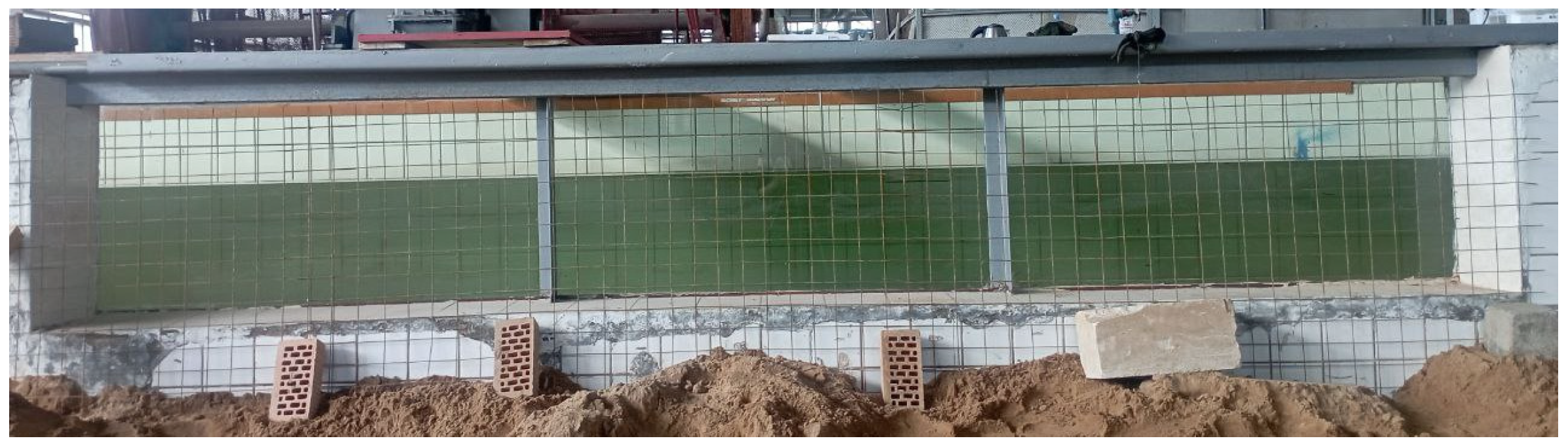
To measure the horizontal displacement of the plate, a metal rod mesh with a cell size of 3 × 3 cm was attached to the side glass wall of the flume (Figure 1).

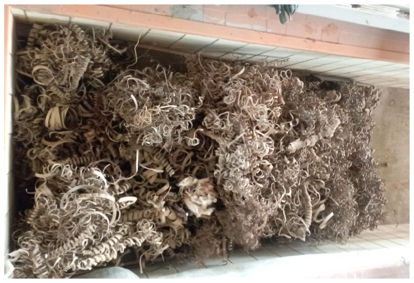
Waves were damped using a damper made of metal filings placed at the rear of the flume (Figure 2). The length of the wave damper corresponded to the maximum wave length.

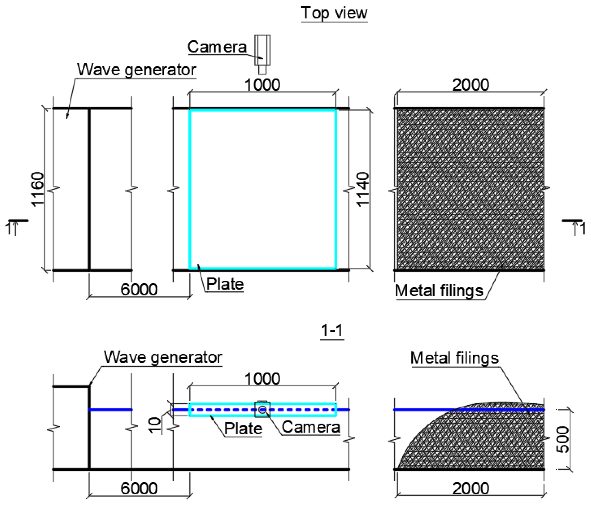
An image of the model is shown in Figure 3.

The system shown in Figure 3 was exposed to regular waves of various periods and lengths (those comparable in dimension to the length of the plate). After that, a camera (and a grid on the glass wall of the flume) was used to record the horizontal displacements of the plate during 1–2 min of wave exposure. The data from the camera was then used to plot graphs showing how the horizontal coordinates of the plate change over time when exposed to various regular waves.

A wave sensor was used to measure the amplitudes of the waves before and after they passed through the floating body.

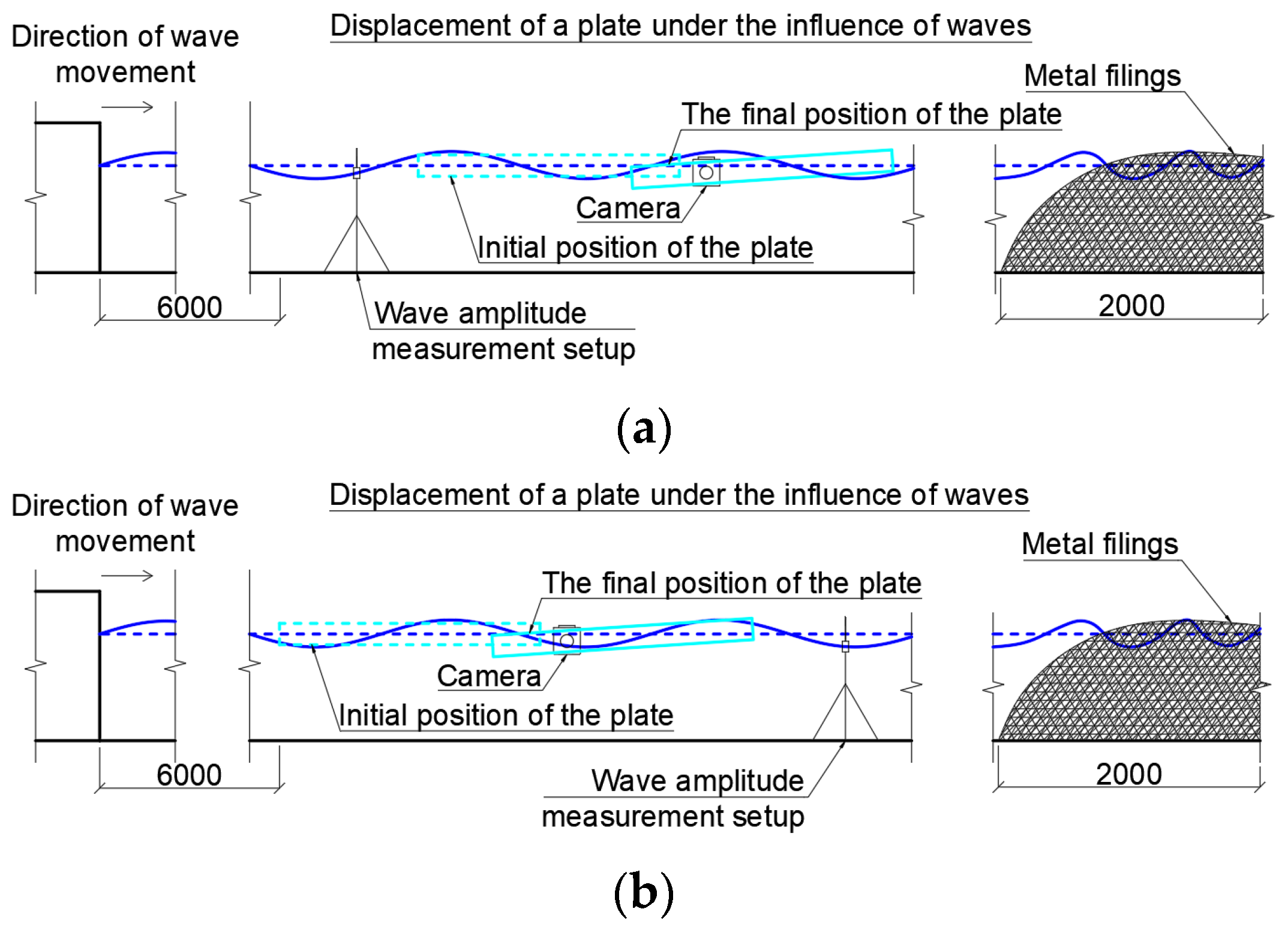
The model’s operation is shown in Figure 4.

After the horizontal displacements of the plate and changes in wave heights were documented for various combinations of periods and wavelengths, the experiment was considered complete.

2.1.2. Selection of Wave Parameters

The scale of the model used in the tests was 1:125 (α = 125). Hydrometeorological data from the Barents Sea [19,20] were taken as the real conditions. All the actual determining parameters from the experiments were converted into model parameters, taking into account the scale and in accordance with the theory of similarity between actual and model objects in the case of wave effects [21].

The range of wave periods at the facility was T_m = 0.5…2 s, the range of wavelengths λ_m was determined by the dispersion law for gravitational waves:

$$\mathsf{\lambda }={\displaystyle \frac{g{T}^2}{2\mathsf{\pi }}}\mathrm{t}\mathrm{h}\left({\displaystyle \frac{2\mathsf{\pi }d}{\mathsf{\lambda }}}\right)$$

(1)

The water depth for the experiment is taken to be d_m = 0.5 m. When d_m = 0.5 m, t_i = 0.01 m, $\mathsf{\rho }$_i = 720 kg/m³, and the density of water is $\mathsf{\rho }$ = 1000 kg/m³, the distance between the bottom of the wave flume and the bottom of the plate is approximately 0.49 m in calm conditions.

At a depth of d_m = 0.5 m and a period of T_m = 0.5 s, the wavelength λ_m according to (1) is equal to 0.39 m. At a depth of d_m = 0.5 m and a period of T_m = 2 s, the wavelength λ_m according to (1) is equal to 4.06 m. Thus, the wavelength range at the facility is λ_m = 0.39…4.06 m.

The experiment was conducted for six possible periods T_m and wavelengths λ_m, presented in

Table 1. Wave parameters selected for the experiment.

Experiment Number	Tm, s	λm, m
1	0.6	0.5
2	0.8	1.0
3	0.9	1.25
4	1.0	1.5
5	1.1	1.75
6	1.2	2.0

. It was necessary to establish how the ratio of wavelengths λ to the horizontal size of the ice floe L affects the attenuation of wave energy with a corresponding decrease in the height of the waves that have passed.

The similarity of model and natural conditions is verified for the case when T_m = 1.2 s and λ_m = 2 m. The average period of natural waves T_n for a storm occurring once every 25 years, according to [19] for the Barents Sea, is equal to T_n = 13.0 s. The natural depth is determined by multiplying d_m by α: d_n = 0.5 × 125 = 62.5 m.

According to (1), the length of natural waves λ_n = 244 m is determined for the selected depth and period. Then:

$${\displaystyle \frac{{\mathsf{\lambda }}_n}{\mathsf{\alpha }}}=1.95 \mathrm{m}\approx {\mathsf{\lambda }}_m=2 \mathrm{m}$$

(2)

The linear relationship between the wavelengths in the experiment and in nature is approximately preserved.

Next, the similarity between T_m and T_n is checked using the Froude criterion Fr [21]:

$$Fr={\displaystyle \frac{L}{g{T}^2}}=const$$

(3)

$${\displaystyle \frac{{\mathsf{\lambda }}_m}{g{T}_m^2}}={\displaystyle \frac{{\mathsf{\lambda }}_n}{g{T}_n^2}}\to T_m\approx \sqrt{{\displaystyle \frac{{\mathsf{\lambda }}_m}{{\mathsf{\lambda }}_n}}}{T}_n=1.18 \mathrm{s}$$

The obtained period is approximately equal to the initially selected one (T_m = 1.2 s); therefore, the calculation is correct.

2.1.3. Self-Similarity

In order for the above conditions to be met, the physical model should be designed so that, with respect to the Froude criterion, all secondary similarity criteria fall within the self-similarity zone. This zone sets the limits of the values of the forces included in the similarity criteria, at which they can be neglected in comparison with the forces of gravity.

Reynolds criterion for compliance with the self-similarity condition [22]:

$${\mathsf{\lambda }}_m>400\sqrt{\mathsf{\nu }{T}_n},$$

(4)

where ν = 1.787 × 10⁻⁶ m²/s is the kinematic viscosity of water at 0 °C.

In order to neglect the influence of surface tension forces on wave processes, restrictions are imposed on the length of the simulated waves during experiments: λ_m > 0.2 m.

The self-similarity condition according to (4):

$${\displaystyle \frac{g{\left(\frac{T_n}{\sqrt{\mathsf{\alpha }}}\right)}^2}{2\mathsf{\pi }}}>400\sqrt{\mathsf{\nu }{T}_n}$$

$${\displaystyle \frac{9.81{\left(\frac{13.0}{\sqrt{125}}\right)}^2}{2\mathsf{\pi }}}=2.11 \mathrm{m}>400\sqrt{1.787\ast {10}^{-6}\ast 13.0}=1.93 \mathrm{m}$$

The Reynolds criterion is within the self-similarity zone.

2.1.4. Selection of Ice Parameters

The main similarity criteria in physical modeling of wave–ice interaction are buoyancy and ice strength.

Buoyancy is ensured by the fact that the density of the experimental ice sheet ${\mathsf{\rho }}_i$ = 720 kg/m³ falls within the density range of natural ice (720–940 kg/m³) [23].

The strength of ice is not considered, since ice floes are considered to be rigid bodies with a high modulus of elasticity, equal to approximately 10 GPa [24].

The behavior of ice floes due to the impact of waves on them is ensured by the equality of the Froude criterion Fr for natural and model parameters:

$$Fr={\displaystyle \frac{v_w^2}{gL}},$$

(5)

where v_w = λ/T is the wave velocity; g = 9.81 m/s² is the acceleration due to gravity.

With λ_m = 2 m, T_m = 1.2 s, L_m = 1 m, λ_n = 244 m, and T_n = 13 s, the natural length of the ice floe L_n according to (5) will be equal to:

$$L_n={L_m\left({\displaystyle \frac{{\mathsf{\lambda }}_n}{{\mathsf{\lambda }}_m}}{\displaystyle \frac{T_m}{T_n}}\right)}^2\approx 130 \mathrm{m}$$

According to [20], ice floes in the Barents Sea can be elongated (ξ < 0.55), oval (0.55 ≤ ξ ≤ 0.85), and rounded (ξ > 0.85), where ξ is the eccentricity of the ice floe:

ξ = L/B

(6)

This work considers rounded ice floes, where the width and length of the ice floe are approximately the same.

The area of ice floe S_i is determined by the formula [20]:

S_i = K₃LB

(7)

where K₃ is the fullness coefficient, showing what part of the area of the described rectangle is occupied by the area of the actual ice floe.

For rounded ice floes, according to [20], K₃ = 0.66.

In order to determine the actual dimensions of a rounded ice floe (with sides $B_n^r$ and $L_n^r$) of the same area as the rectangular one used in the experiment, B_n and L_n should be divided by $\sqrt{K_3}$ = $\sqrt{0.66}$ = 0.812. Thus, $L_n^r$ = 130/0.812 = 160 m.

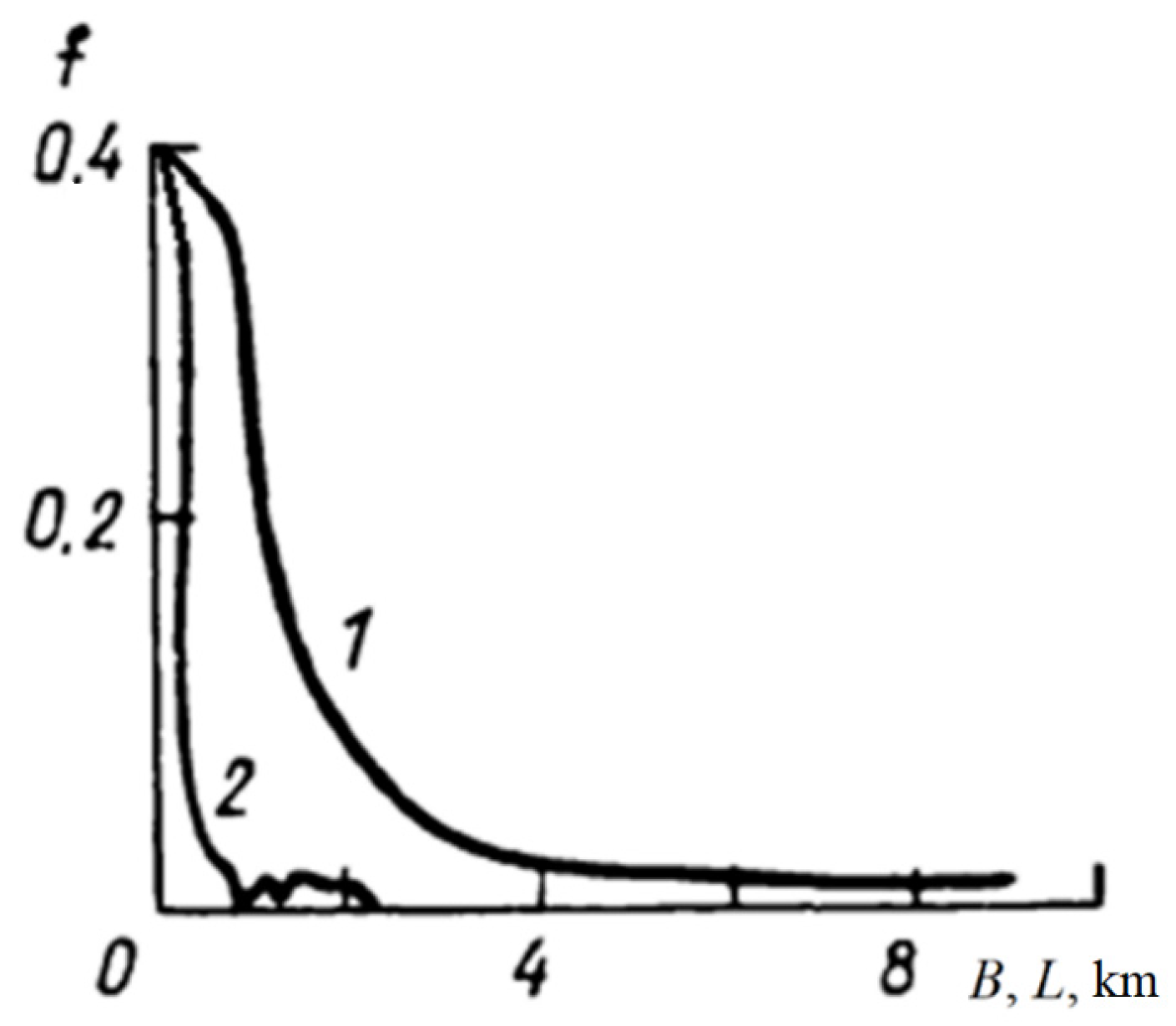
The width of the rounded ice floe $B_n^r$ is determined according to Figure 5 [20]. In Figure 5, f is a dimensionless ice size distribution function that reflects the proportion of ice floes of a given size in the Barents Sea.

With a length $L_n^r$ = 160 m, the width of a rounded ice floe $B_n^r$ according to Figure 5 is approximately $B_n^r$ = 175 m. The selected dimensions satisfy the average eccentricity for rounded ice floes in the Barents Sea, equal to ξ_ave = 0.91 [20] and determined by (6) as:

$${\mathsf{\xi }}_{\mathit{ave}} = L_n^r/B_n^r=160/175=0.91$$

The width of a rectangular ice floe B_n in this case will be determined as B_n = 175 × 0.812 = 143 m.

The model width of the ice floe B_m according to (2):

B_m = B_n/α = 143/125 ≈ 1.14 m

The model length of the ice floe L_m according to (2):

L_m = L_n/α = 130/125 ≈ 1.0 m

The values obtained are identical to the dimensions of the plate selected for the experiments.

2.2. Numerical Model

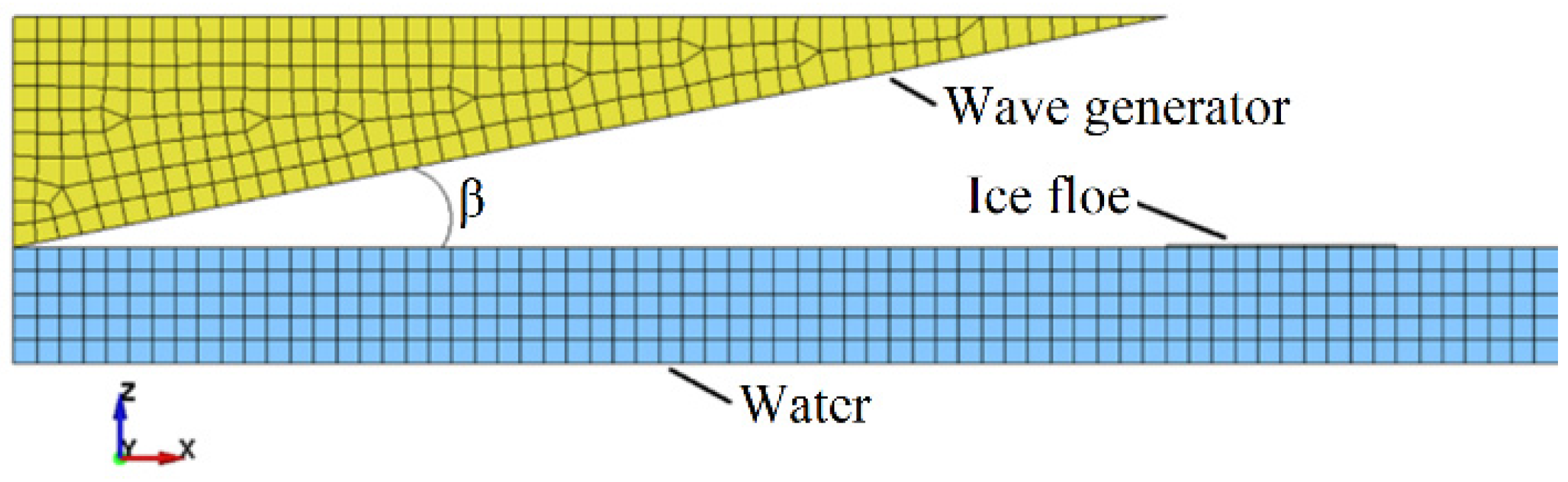
Calculations with the same initial data as in the experiment were performed in a numerical model implemented in the LS-DYNA code (Figure 6).

The main methods for modeling water in LS-DYNA include Computational Fluid Dynamics (CFD), Smoothed Particle Hydrodynamics (SPH), and Arbitrary Lagrangian–Eulerian (ALE) method.

The CFD method is a powerful tool for simulating water and surface waves, enabling a detailed analysis of the dynamic behavior of fluids under various physical conditions. To create realistic water models, the Navier–Stokes equations are used, which describe the motion of a viscous fluid. The method is based on continuous remeshing of the model grid, automatically determining a high-density grid where necessary and a coarser one in less critical areas.

The SPH method is a gridless Lagrangian numerical method used to simulate fluid motion. The SPH method allows for fluid simulation without the use of a traditional mesh, making it particularly useful for problems involving large deformations and complex free surfaces, such as surface waves. The motion of water is governed by the equation of state.

The ALE method is a combination of the Euler and Lagrangian methods.

In the Lagrangian method, the analysis focuses on individual particles of the medium that follow their own trajectories. In this approach, the state of each particle is tracked, including its displacement, velocity, and deformations. Structural analyses are often performed using the finite element method. This is most suitable for systems where it is important to study the behavior of individual particles and the change in their characteristics over time.

The Euler method, on the other hand, focuses on fixed points in space through which material particles pass. Here, the focus is on changes in physical quantities, such as velocity and deformation, at these stationary points. This method is suitable for situations where it is important to understand how changes propagate through the medium, such as in fluid or gas flow modeling.

Water motion in the ALE method is also governed by the equation of state.

According to studies by J. Xu, 2015 [25], D. Varas, 2017 [26], Z. Cai, 2021 [27], and J. Behnen, 2021 [28], the most accessible method for numerically modeling the interaction between waves and free-floating bodies is the ALE method, since it is less resource-intensive compared to the SPH method and less technically complex to use compared to the CFD method, while still providing sufficiently accurate calculation results.

For this reason, the numerical model presented in this article employs the Euler–Lagrange approach.

The dynamic viscosity coefficient of water μ_d was taken to be 0.001 Pa·s.

To create waves in the model, a rigid body with a triangular profile and an angle of inclination to the water surface β equal to β = tg(2h_I/λ) is used (Figure 6). The motion of the body is described by periodic upward and downward movements, during which the body descends into the water to a depth equal to h_I and rises, which leads to the generation of waves. The law of motion of the wave generator:

$$f\left(t\right)={\displaystyle \frac{1}{2}}{h}_I\cos \left(2\mathsf{\pi }{\displaystyle \frac{t}{T}}\right)$$

(8)

Model dimensions: length—20 m; width—0.1 m; height—2 m (water depth—0.5 m; air space height—1.5 m). Finite element size—0.1 m. The floating body is located at a distance equal to the wavelength from the center of wave generation.

A more detailed description of the numerical model, as well as its verification for wave and ice loads, is presented in the works of M.S. Afonyushkin and I.G. Kantarzhi, 2024 [29] and 2025 [30].

2.3. Analytical Model

To calculate the dependence of h_T/h_I on λ/L, an analytical model based on the theoretical analysis of the interaction of waves and floating breakwaters from the work of J.J. Stoker, 1953 [31] is used. Its essence, in the context of the interaction of waves with freely floating rigid bodies, is that the components of the plate’s motion are considered as:

$$\left\{\begin{array}{c}\overline{u}\left(x,t\right)=\overline{x}\left(x\right)e^{i\mathsf{\omega }t},\\ \overline{w}\left(x,t\right)=\overline{\mathsf{\sigma }}\left(x\right)e^{i\mathsf{\omega }t},\\ \overline{v}\left(x,t\right)=\overline{y}\left(x\right)e^{i\mathsf{\omega }t},\end{array}\right.$$

(9)

where $\overline{u}$, $\overline{v}$, and $\overline{w}$ are the functions of the horizontal, vertical, and rotational motion of the plate, respectively; $\overline{x}$, $\overline{y}$, and $\overline{\sigma }$ are constants representing the complex amplitudes of these vibration components; ω = 2π/T is the circular frequency of the waves.

Thus, for the free wave surface function η(x, t) according to [31], we have:

$$\mathsf{\eta }\left(x,t\right)=\left[\overline{y}+\left(x-\overline{x}\right)\overline{\mathsf{\sigma }}\right]e^{i\mathsf{\omega }t}$$

(10)

Since this analytical method is based on linear wave theory for small amplitude waves, the horizontal component of the oscillations $\overline{x}$ is not taken into account:

$$\mathsf{\eta }\left(x,t\right)=\left[\overline{y}+x\overline{\mathsf{\sigma }}\right]e^{i\mathsf{\omega }t}$$

(11)

Bernoulli’s equation for determining hydrodynamic pressure is as follows:

$$p\left(x,t\right)=-\mathsf{\rho }\left({\displaystyle \frac{\partial \mathsf{\Phi }\left(x,t\right)}{\partial t}}+g\mathsf{\eta }\left(x,t\right)\right),$$

(12)

where p(x, t) is the wave hydrodynamic pressure; Φ(x, t) is the function of the water velocity potential on the free surface.

Since the functions Φ(x, t) and η(x, t) represent harmonic oscillations, they can be represented as:

$$\left\{\begin{array}{c}\mathsf{\Phi }\left(x,t\right)=\mathsf{\varphi }\left(x\right)e^{i\mathsf{\omega }t},\\ \mathsf{\eta }\left(x,t\right)=v\left(x\right)e^{i\mathsf{\omega }t},\end{array}\right.$$

(13)

where ϕ(x) is the complex velocity potential function; v(x) is the complex free surface equation function, which, taking into account (11), is equal to:

$$v\left(x\right)=\overline{y}+x\overline{\mathsf{\sigma }}$$

(14)

For a problem with harmonic waves traveling from $x=-\infty$ to $x=+\infty$, where the ice floe occupies the interval from x = 0 to x = L, the conditions for Φ(x, t) and η(x, t) in accordance with [31] are written as follows:

$${\displaystyle \frac{{\partial }^2\mathsf{\varphi }\left(x\right)}{\partial x^2}}+{\displaystyle \frac{{\mathsf{\omega }}^2}{gd}}\mathsf{\varphi }\left(x\right)=0, x\le 0, x\ge L$$

(15)

$${\displaystyle \frac{{\partial }^2\mathsf{\varphi }\left(x\right)}{\partial x^2}}+{\displaystyle \frac{i\mathsf{\omega }}{d}}v\left(x\right)=0, 0\le x\le L$$

(16)

From (16) we determine ${\partial }^2\mathsf{\varphi }\left(x\right)/\partial x^2$, which, taking into account (14), is calculated as:

$${\displaystyle \frac{{\partial }^2\mathsf{\varphi }\left(x\right)}{\partial x^2}}=-{\displaystyle \frac{i\mathsf{\omega }}{d}}\left(\overline{y}+x\overline{\mathsf{\sigma }}\right)$$

(17)

It follows that the function ϕ(x) is a cubic polynomial:

$$\mathsf{\varphi }\left(x\right)=-{\displaystyle \frac{i\mathsf{\omega }}{d}}\left({\displaystyle \frac{\overline{\mathsf{\sigma }}{x}^3}{6}}+{\displaystyle \frac{\overline{y}{x}^2}{2}}\right)+\mathsf{\gamma }x+\mathsf{\delta },$$

(18)

where γ and δ are unknown constants.

To determine the function ϕ(x) for x ≤ 0, x ≥ L, we need to find the general solution of Equation (15), which has the form [31]:

$$\mathsf{\varphi }\left(x\right)=A{e}^{-ikx}+B{e}^{ikx}, x\le 0, x\ge L,$$

(19)

where k = 2π/λ is the wave number; $A{e}^{-ikx}$ is a term of the equation representing a wave moving in the direction of the x-axis; and $B{e}^{ikx}$ is a term of the equation representing a wave moving in the opposite direction.

Given that in this model the direction of wave propagation coincides with the x-axis, we rewrite (19) as:

$$\mathsf{\varphi }\left(x\right)=\left\{\begin{array}{c}{A}_I{e}^{-ikx}+A_R{e}^{ikx}, x\le 0,\\ A_T{e}^{-ikx}, x\ge L,\end{array}\right.$$

(20)

where A_I = h_I/2 is the amplitude of the incident waves; A_R is the amplitude of the reflected waves; A_T is the amplitude of the transmitted waves.

Boundary conditions at x = 0 (end of the ice floe close to the incident waves):

$$\mathsf{\varphi }\left(0\right)=A_I+A_R$$

(21)

$${\displaystyle \frac{\partial \mathsf{\varphi }\left(0\right)}{\partial x}}=ik\left(A_R-A_I\right)$$

(22)

Boundary conditions at x = L (end of the ice floe far from the incident waves):

$$\mathsf{\varphi }\left(L\right)=A_T{e}^{-ikL}$$

(23)

$${\displaystyle \frac{\partial \mathsf{\varphi }\left(L\right)}{\partial x}}=-ik{A}_T{e}^{-ikL}$$

(24)

These four Equations (21)–(24) are not sufficient to determine the six constants: γ, δ, $\overline{y}$, $\overline{\mathsf{\sigma }}$, A_R, and A_T. To do this, we will use the equations of dynamics of a floating rigid body:

$$\left\{\begin{array}{c}F=M\dot{v},\\ S=J\dot{w},\end{array}\right.$$

(25)

where F is the total vertical force acting on the plate; M is the mass of the plate; $\dot{v}$ is the vertical acceleration of the center of gravity of the plate; S is the torque acting on the plate; J is the mass moment of inertia of the plate; $\dot{w}$ is the angular acceleration.

Equation (25), taking into account (9), can be represented as:

$${\int }_0^{L}p\left(x,t\right)dx=M{\displaystyle \frac{{\partial }^2\overline{v}(x,t)}{\partial t^2}}=-M{\mathsf{\omega }}^2\overline{y}{e}^{i\mathsf{\omega }t}$$

(26)

$${\int }_0^{L}p\left(x,t\right)xdx=J{\displaystyle \frac{{\partial }^2\overline{w}(x,t)}{\partial t^2}}=-J{\mathsf{\omega }}^2\overline{\sigma }{e}^{i\mathsf{\omega }t}$$

(27)

Since the pressure p(x, t) is given by Formula (12), taking into account (11), (13) and (18), we have:

$$p\left(x,t\right)=-\mathsf{\rho }\left(i\mathsf{\omega }\left(-{\displaystyle \frac{i\mathsf{\omega }}{d}}\left({\displaystyle \frac{\overline{\mathsf{\sigma }}{x}^3}{6}}+{\displaystyle \frac{\overline{y}{x}^2}{2}}\right)+\mathsf{\gamma }x+\mathsf{\delta }\right)+g\left(\overline{y}+x\overline{\mathsf{\sigma }}\right)\right)e^{i\mathsf{\omega }t}$$

(28)

Taking into account (26) and (27), we integrate the left sides of (28) and reduce both sides by $e^{i\mathsf{\omega }t}$:

$$\begin{array}{c}\mathsf{\gamma }\left({\displaystyle \frac{1}{2}}i\mathsf{\omega }\mathsf{\rho }{L}^2\right)+\mathsf{\delta }\left(i\mathsf{\omega }\mathsf{\rho }L\right)+\overline{y}\left(g\mathsf{\rho }L+{\displaystyle \frac{1}{6}}{\displaystyle \frac{L^3{\mathsf{\rho }\mathsf{\omega }}^2}{d}}+M{\mathsf{\omega }}^2\right)+\\ +\overline{\mathsf{\sigma }}\left({\displaystyle \frac{1}{2}}{L}^{2}g\mathsf{\rho }+{\displaystyle \frac{1}{24}}{\displaystyle \frac{L^4{\mathsf{\rho }\mathsf{\omega }}^2}{d}}\right)=0\end{array}$$

(29)

$$\begin{array}{c}\mathsf{\gamma }\left({\displaystyle \frac{1}{3}}i\mathsf{\omega }\mathsf{\rho }{L}^3\right)+\mathsf{\delta }\left({\displaystyle \frac{1}{2}}i\mathsf{\omega }\mathsf{\rho }{L}^2\right)+\overline{y}\left({\displaystyle \frac{1}{2}}g\mathsf{\rho }{L}^2+{\displaystyle \frac{1}{8}}{\displaystyle \frac{L^4{\mathsf{\rho }\mathsf{\omega }}^2}{d}}\right)+\\ +\overline{\mathsf{\sigma }}\left({\displaystyle \frac{1}{3}}{L}^{3}g\mathsf{\rho }+{\displaystyle \frac{1}{30}}{\displaystyle \frac{L^5{\mathsf{\rho }\mathsf{\omega }}^2}{d}}+J{\mathsf{\omega }}^2\right)=0\end{array}$$

(30)

Taking into account the six boundary conditions (21)–(24), (29) and (30), we obtain six linear equations from (18) to determine the six unknown constants: γ, δ, $\overline{y}$, $\overline{\mathsf{\sigma }}$, A_R, and A_T.

The final system of equations is as follows:

$$\left\{\begin{array}{c}\begin{array}{c}\mathsf{\gamma }\ast \left(0\right)+\mathsf{\delta }\ast \left(1\right)+\overline{y}\ast \left(0\right)+\overline{\mathsf{\sigma }}\ast \left(0\right)+A_R\ast \left(-1\right)+A_T\ast \left(0\right)=A_I\\ \mathsf{\gamma }\ast \left({\displaystyle \frac{i}{k}}\right)+\mathsf{\delta }\ast \left(0\right)+\overline{y}\ast \left(0\right)+\overline{\mathsf{\sigma }}\ast \left(0\right)+A_R\ast \left(1\right)+A_T\ast \left(0\right)=A_I\\ \begin{array}{c}\mathsf{\gamma }\ast \left(L\right)+\mathsf{\delta }\ast \left(1\right)+\overline{y}\ast \left(-{\displaystyle \frac{i\mathsf{\omega }}{d}}{\displaystyle \frac{L^2}{2}}\right)+\overline{\mathsf{\sigma }}\ast \left(-{\displaystyle \frac{i\mathsf{\omega }}{d}}{\displaystyle \frac{L^3}{6}}\right)+A_R\ast \left(0\right)+A_T\ast (-e^{-ikL})=0\\ \mathsf{\gamma }\ast \left({\displaystyle \frac{i}{k}}\right)+\mathsf{\delta }\ast \left(0\right)+\overline{y}\ast \left({\displaystyle \frac{\mathsf{\omega }}{kd}}L\right)+\overline{\mathsf{\sigma }}\ast \left({\displaystyle \frac{\mathsf{\omega }}{kd}}{\displaystyle \frac{L^2}{2}}\right)+A_R\ast \left(0\right)+A_T\ast (-e^{-ikL})=0\\ \begin{array}{c}\mathsf{\gamma }\ast \left({\displaystyle \frac{1}{2}}i\mathsf{\omega }\mathsf{\rho }{L}^2\right)+\mathsf{\delta }\ast \left(i\mathsf{\omega }\mathsf{\rho }L\right)+\overline{y}\left(g\mathsf{\rho }L+{\displaystyle \frac{1}{6}}{\displaystyle \frac{L^3{\mathsf{\rho }\mathsf{\omega }}^2}{d}}+M{\mathsf{\omega }}^2\right)+\\ +\overline{\mathsf{\sigma }}\left({\displaystyle \frac{1}{2}}{L}^{2}g\mathsf{\rho }+{\displaystyle \frac{1}{24}}{\displaystyle \frac{L^4{\mathsf{\rho }\mathsf{\omega }}^2}{d}}\right)+A_R\ast \left(0\right)+A_T\ast \left(0\right)=0\end{array}\end{array}\end{array}\\ \gamma \ast \left({\displaystyle \frac{1}{3}}i\mathsf{\omega }\mathsf{\rho }{L}^3\right)+\mathsf{\delta }\ast \left({\displaystyle \frac{1}{2}}i\mathsf{\omega }\mathsf{\rho }{L}^2\right)+\overline{y}\left({\displaystyle \frac{1}{2}}g\mathsf{\rho }{L}^2+{\displaystyle \frac{1}{8}}{\displaystyle \frac{L^4{\mathsf{\rho }\mathsf{\omega }}^2}{d}}\right)+\\ +\overline{\mathsf{\sigma }}\left({\displaystyle \frac{1}{3}}{L}^{3}g\mathsf{\rho }+{\displaystyle \frac{1}{30}}{\displaystyle \frac{L^5{\mathsf{\rho }\mathsf{\omega }}^2}{d}}+J{\mathsf{\omega }}^2\right)+A_R\ast \left(0\right)+A_T\ast \left(0\right)=0\end{array}\right.$$

(31)

The unknown members of this system of equations are determined using Cramer’s method:

$$\mathsf{\gamma }={\displaystyle \frac{{\Delta }_{\mathsf{\gamma }}}{\Delta }},\mathsf{\delta }={\displaystyle \frac{{\Delta }_{\mathsf{\delta }}}{\Delta }},\overline{y}={\displaystyle \frac{{\Delta }_{\overline{y}}}{\Delta }},\overline{\mathsf{\sigma }}={\displaystyle \frac{{\Delta }_{\overline{\mathsf{\sigma }}}}{\Delta }},A_R={\displaystyle \frac{{\Delta }_R}{\Delta }},A_T={\displaystyle \frac{{\Delta }_T}{\Delta }},$$

(32)

where Δ is the determinant of the matrix of the system of Equation (23); Δ_γ, Δ_δ, ${\Delta }_{\overline{y}}$, ${\Delta }_{\overline{\mathsf{\sigma }}}$, Δ_R, and Δ_T are the determinants of the corresponding unknown variables of the system of Equation (31).

The found values of amplitudes A_R and A_T are checked according to the formula:

$$C_R^2+C_T^2=1,$$

(33)

where $C_R=\left|A_R\right|/\left|A_I\right|$ and $C_T=\left|A_T\right|/\left|A_I\right|$ are the coefficients of reflection and transmission of wave energy, respectively.

The height of the transmitted waves h_T in this case is determined as $h_T=2\left|A_T\right|$.

3. Results

3.1. Analysis of Physical Modeling Results

The experiment was conducted for six model wave periods: $T_m^{\mathsf{\lambda }/L=0.5}=0.63 \mathrm{s}$, $T_m^{\mathsf{\lambda }/L=1.0}=0.81 \mathrm{s}$, $T_m^{\mathsf{\lambda }/L=1.25}=0.92 \mathrm{s}$, $T_m^{\mathsf{\lambda }/L=1.5}=1.03 \mathrm{s}$, $T_m^{\mathsf{\lambda }/L=1.75}=1.10 \mathrm{s}$, and $T_m^{\mathsf{\lambda }/L=2.0}=1.18 \mathrm{s}$.

When converting the model data to actual data using a scale factor α = 125, the following values of actual wave periods were obtained: $T_n^{\mathsf{\lambda }/L=0.5}=7 \mathrm{s}$, $T_n^{\mathsf{\lambda }/L=1.0}=9 \mathrm{s}$, $T_n^{\mathsf{\lambda }/L=1.25}=10 \mathrm{s}$, $T_n^{\mathsf{\lambda }/L=1.5}=11 \mathrm{s}$, $T_n^{\mathsf{\lambda }/L=1.75}=12 \mathrm{s}$, and $T_n^{\mathsf{\lambda }/L=2.0}=13 \mathrm{s}$.

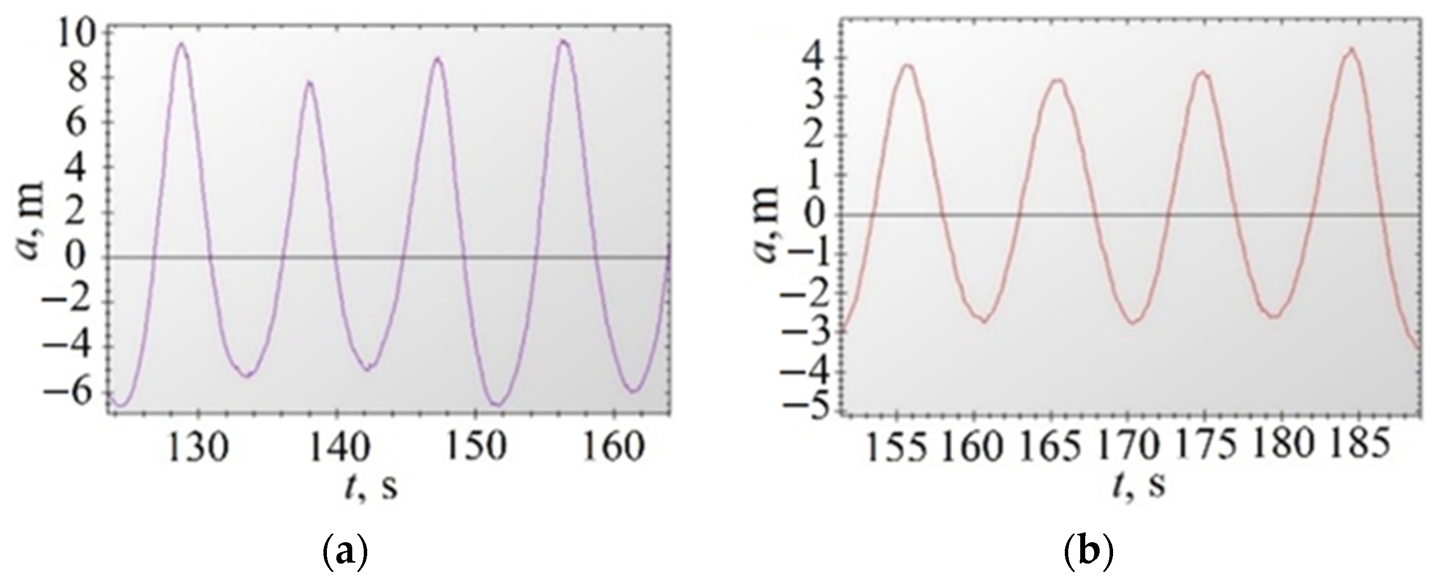
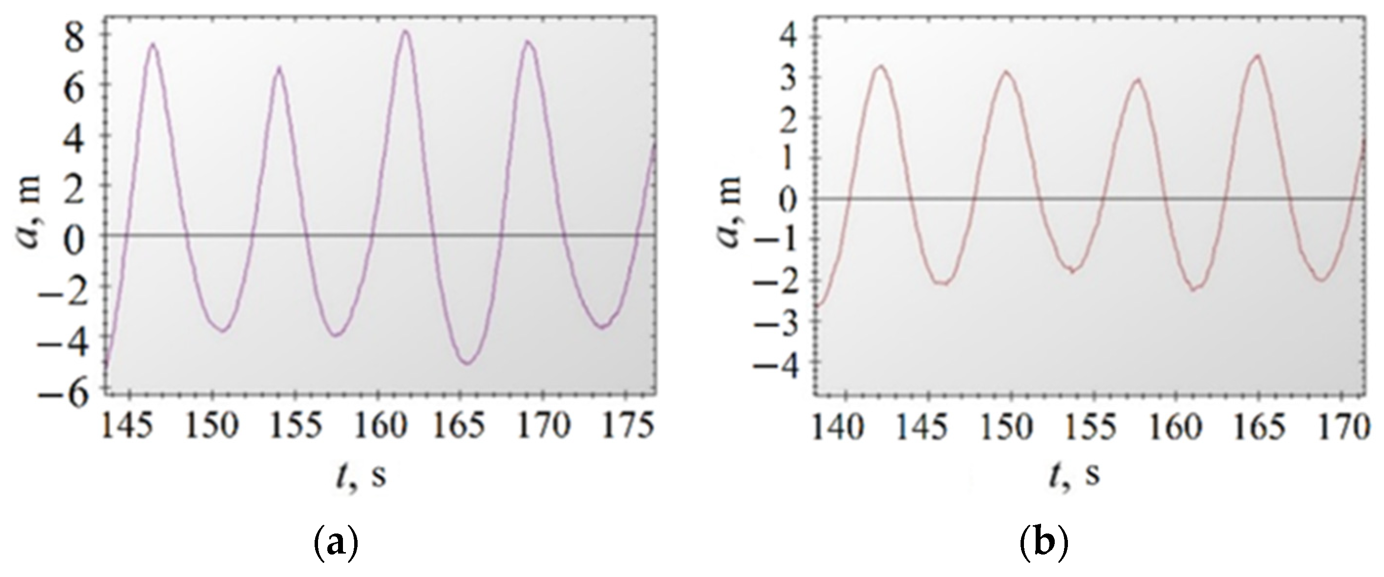
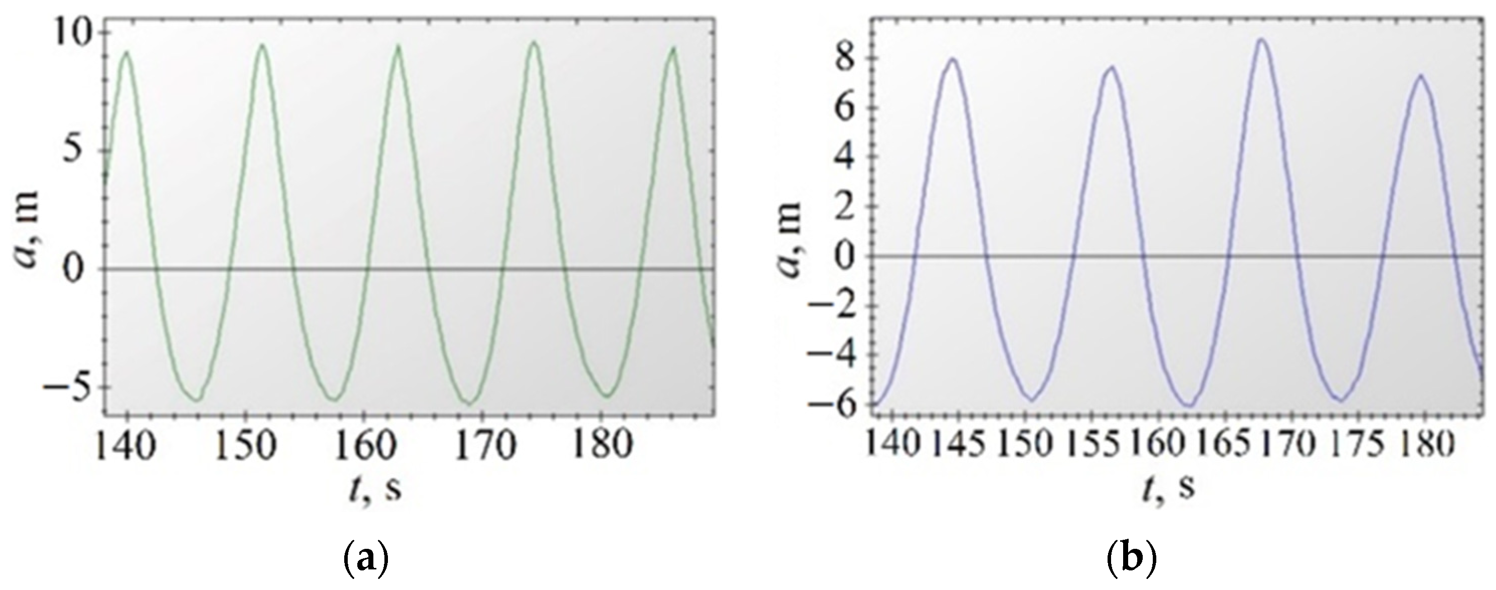
Figure 7, Figure 8 and Figure 9 show the results of changes in wave amplitude a as a function of time t when waves pass through a freely floating plate for three modes of interaction between waves and the plate: at λ/L = 0.5, at λ/L = 1.0, and at λ/L = 2.0.

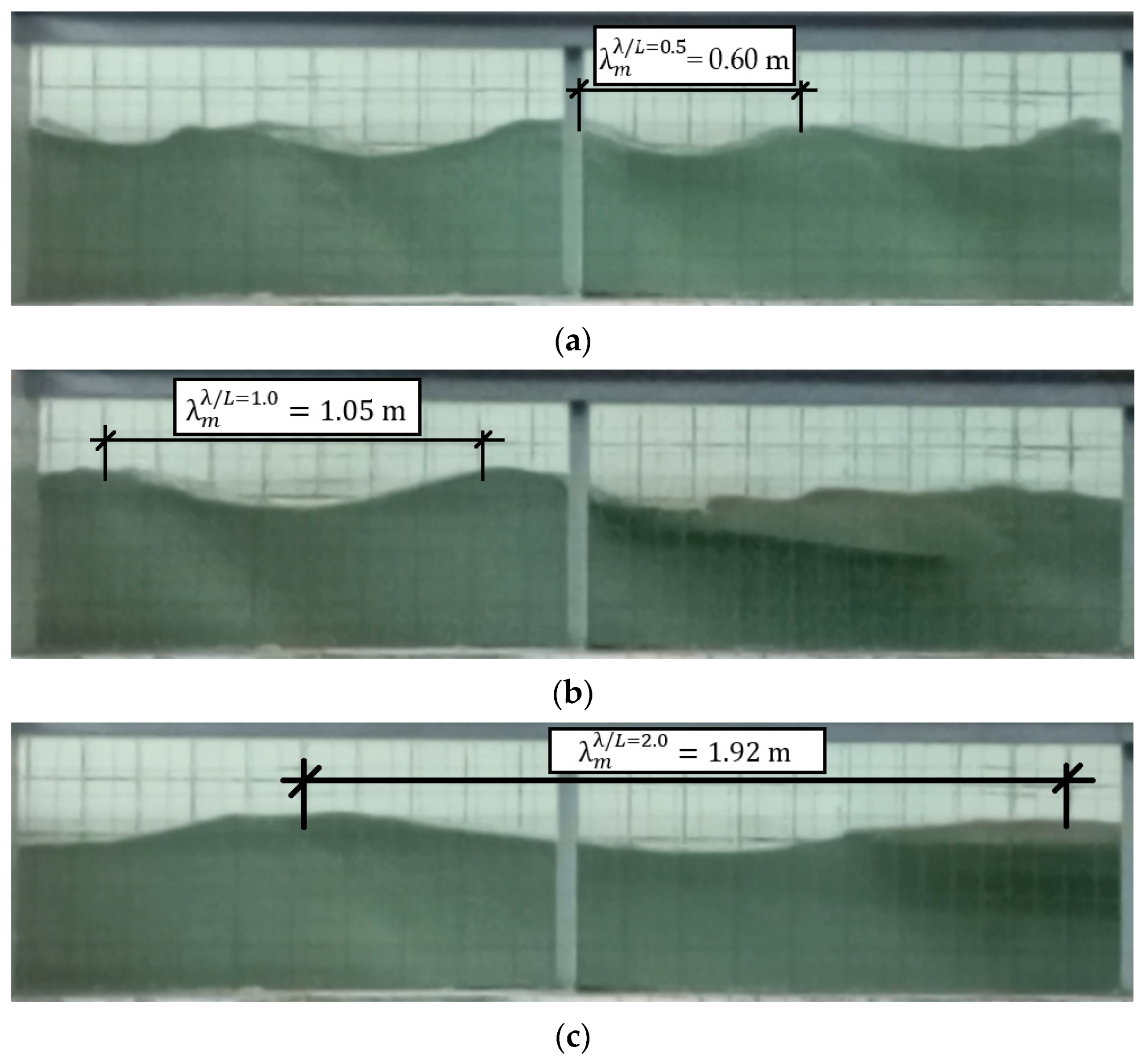
The lengths of the generated model waves at the corresponding λ/L ratios were obtained as follows—${\lambda }_m^{\mathsf{\lambda }/L=0.5}=0.60 \mathrm{m}$, ${\lambda }_m^{\mathsf{\lambda }/L=1.0}=1.05 \mathrm{m}$, ${\lambda }_m^{\mathsf{\lambda }/L=1.25}=1.30 \mathrm{m}$, ${\lambda }_m^{\mathsf{\lambda }/L=1.5}=1.59 \mathrm{m}$, ${\lambda }_m^{\mathsf{\lambda }/L=1.75}=1.78 \mathrm{m}$, and ${\lambda }_m^{\mathsf{\lambda }/L=2.0}=1.92 \mathrm{m}$—which is in fairly good agreement with the initially established values: 0.5 m, 1.0 m, 1.25 m, 1.5 m, 1.75 m, and 2.0 m, respectively. Figure 10 shows the resulting wavelengths for three modes of interaction between the waves and the freely floating plate at λ/L = 0.5, at λ/L = 1.0, and at λ/L = 2.0.

Table 2. Change in wave height when waves pass through a free-floating plate.

λ/L	hI,n, m	hT,n, m	hT,n/hI,n
0.5	11.3	5.2	0.45
1.0	14.0	6.3	0.46
1.25	14.3	9.0	0.63
1.5	14.6	10.4	0.71
1.75	14.9	12.2	0.82
2.0	15.0	13.6	0.91

shows the actual wave heights before (h_I,n) and after (h_T,n) the waves passed through the plate for each of the calculated cases, as well as their calculated ratio h_T,n/h_I,n.

Based on the results of the experiment, the following conclusions can be drawn:

• At λ/L = 2.0, the wave height when waves pass through a thin plate remains virtually unchanged because, as expected, the plate simply floats on the waves, offering little resistance to their movement.
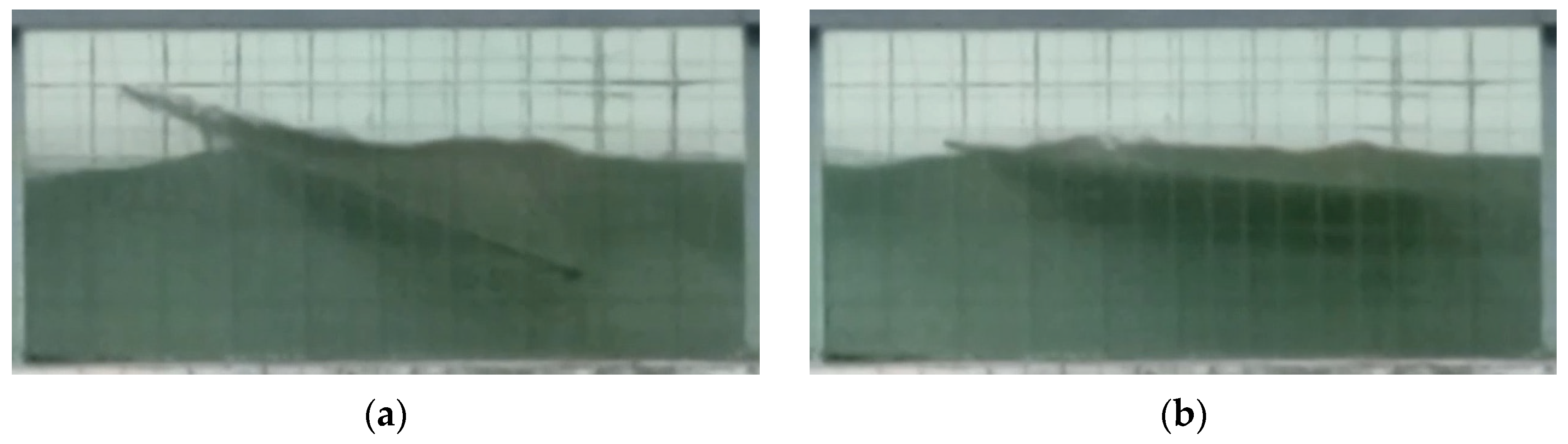
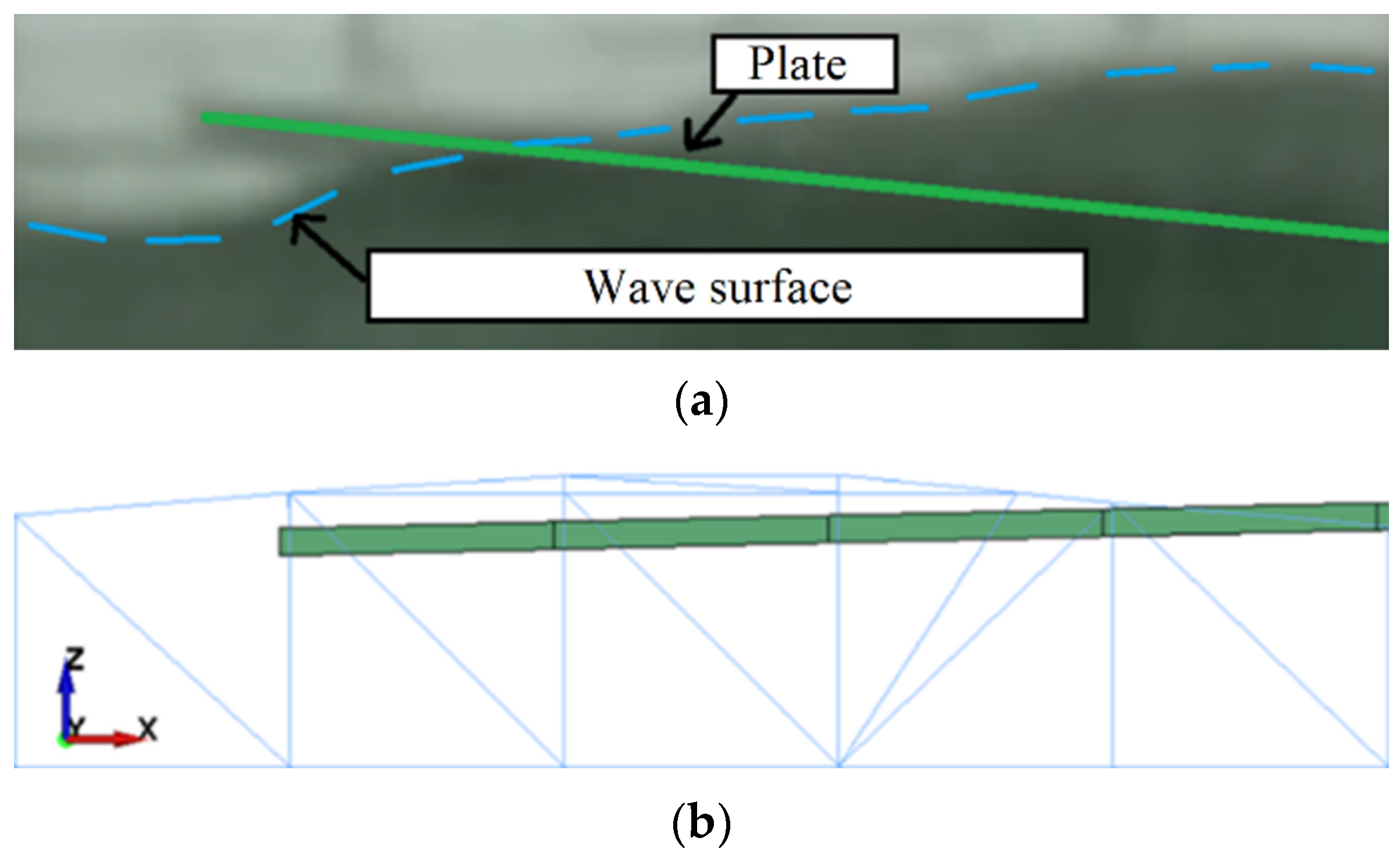
• At λ/L = 1.0, the height of the waves passing through the thin plate decreases by approximately 2 times. This can be explained by the fact that at this mode, both adjacent wave crests coincide with the coordinates of the free ends of the board. Without taking into account attenuation, the plate in this position should move strictly vertically, but due to wave attenuation, its rear part begins to tilt downwards, and the front part constantly interacts with the incident waves. As a result, the board overturns and partially submerges into the water at the rear end (Figure 11a). Due to this interaction, the front edge of the plate takes on the entire force of the incident waves, as a result of which real ice in this mode will break into smaller fragments, leveling the effect of such interaction and contributing to the transition to the mode at λ/L > 1.0.
• In the λ/L = 0.5 mode, the height of the waves passing through the thin plate also decreases by approximately 2 times. At the same time, due to the difference in wave amplitudes in front and behind, the rear part of the plate partially submerges in water, but does not go completely under water, since in the central zone the equilibrium of the plate is maintained by a wave with a larger amplitude than at its rear edge (Figure 11b).
• For the modes λ/L = 1.25, λ/L = 1.5, and λ/L = 1.75, a smooth transition was observed from the λ/L = 1.0 mode to the λ/L = 2.0 mode.

It is also important to note that the obtained values of h_T,n/h_I,n, equal to approximately 0.5 for the modes λ/L = 0.5 and λ/L = 1.0, are consistent with the experimental data from [8], where the authors, conducting laboratory studies to determine the dependence of h_T/h_I on λ/L, obtained average values of h_T/h_I = 0.5 at ratios λ/L = 0.56 and λ/L = 1.00.

Table 3. The values of v_i/v_w found based on the results of physical modeling.

λ/L	Tm, s	λm, m	vi, mm/s	vw, mm/s	vi/vw
0.60	0.63	0.60	95	952	0.100
1.05	0.81	1.05	0	1296	0
1.30	0.92	1.30	71	1413	0.050
1.59	1.03	1.59	91	1544	0.059
1.78	1.10	1.78	87	1618	0.054
1.92	1.18	1.92	84	1627	0.052

lists all the v_i/v_w values obtained for all wave-plate interaction modes, based on the results of physical modeling.

3.2. Analysis of Numerical Simulation Results

The calculation was performed for wave periods T equal to 0.40 s, 0.60 s, 0.70 s, 0.80 s, 1.00 s, 1.20 s, and 1.57 s. Wave lengths λ according to (1) are taken as follows: 0.25 m, 0.50 m, 0.75 m, 1.00 m, 1.50 m, 2.00 m, 3.00 m. Calculations of wave velocities v_w = λ/T and ice velocities v_i, as well as the ratios h_T/h_I and v_i/v_w at d = 0.5 m, L = 1 m, and h_I = 0.05…0.10 m (so that the wave steepness is no more than 0.2) depending on the previously specified wave characteristics λ and T, are presented in

Table 4. The values of v_i/v_w and h_T/h_I found based on the results of numerical modeling.

λ/L	T, s	λ, m	vi, mm/s	vw, mm/s	vi/vw	hT/hI
0.25	0.40	0.25	75	625	0.120	0.10
0.50	0.60	0.50	95	833	0.114	0.30
0.75	0.70	0.75	114	1071	0.106	0.40
1.00	0.80	1.00	0	1250	0	0.50
1.50	1.00	1.50	91	1500	0.061	0.70
2.00	1.20	2.00	84	1667	0.050	0.90
3.00	1.57	3.00	61	1911	0.032	0.95

.

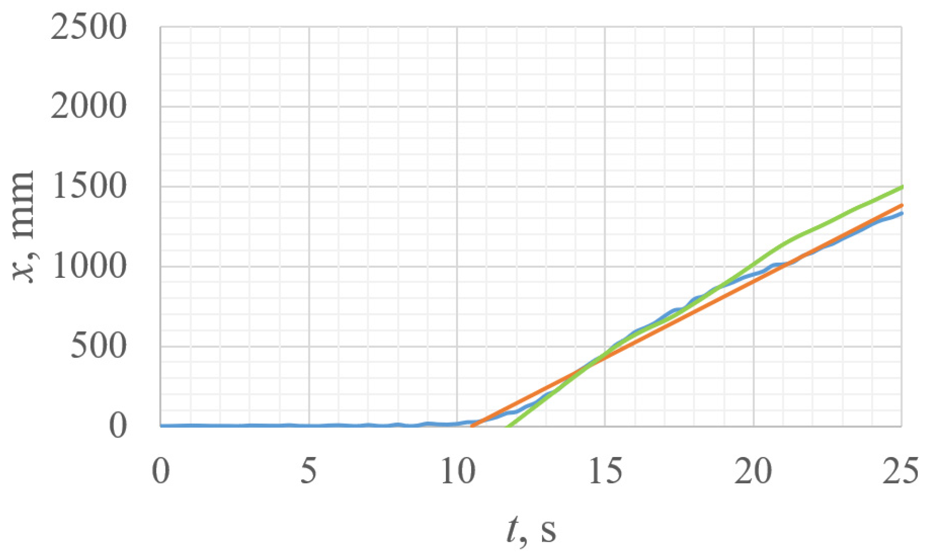
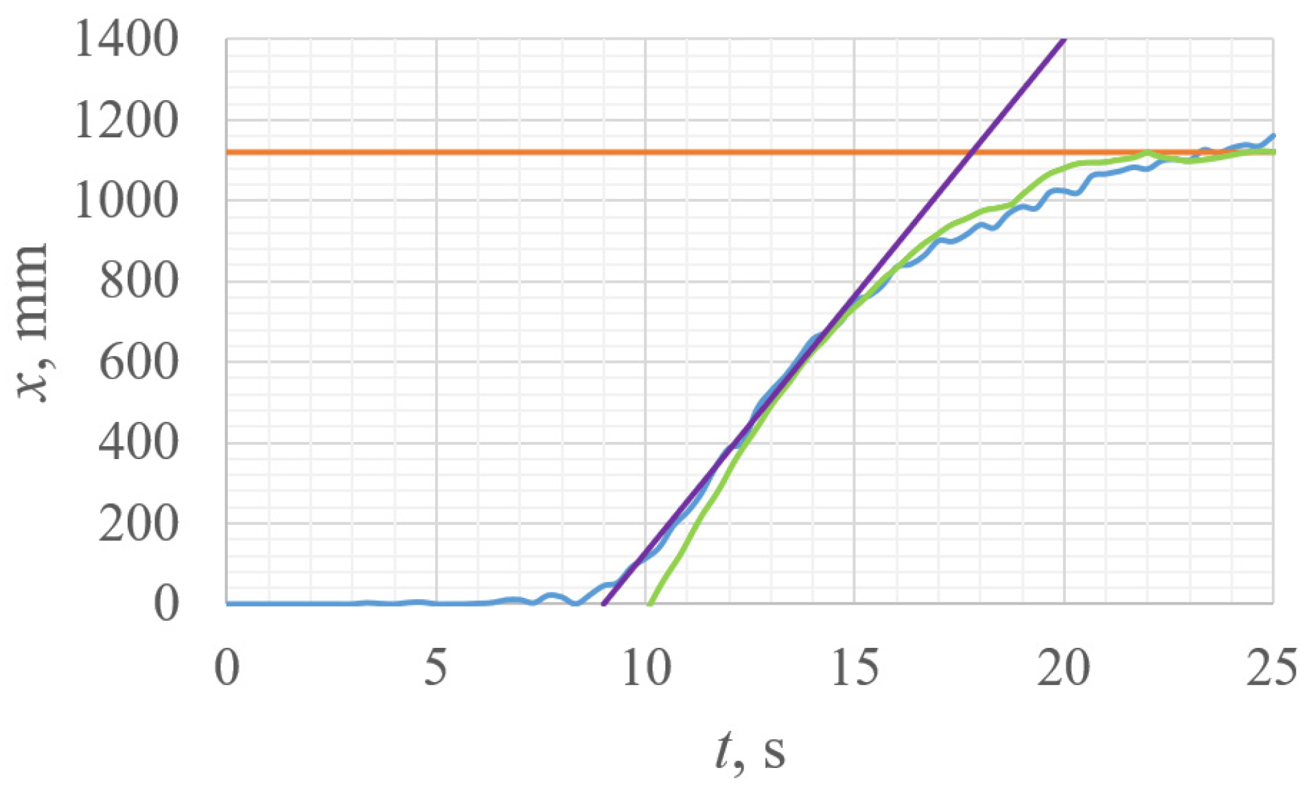
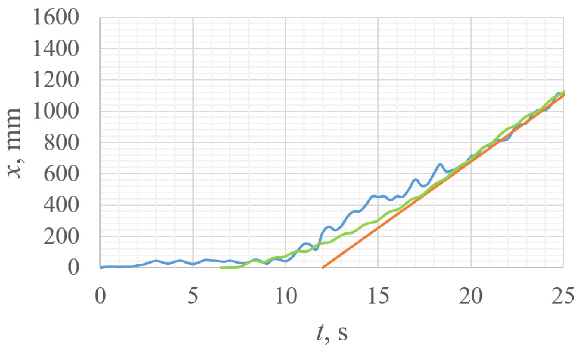
Figure 12, Figure 13 and Figure 14 show the dependencies of the horizontal displacement of the plate x on time t in the numerical model, compared with similar values obtained from the experimental results (using a video recording device) for the modes of interaction between the waves and the plate at λ/L = 0.5, λ/L = 1.0, and λ/L = 2.0.

The value $v_i^{\mathsf{\lambda }/L=2.0} = 84 \mathrm{m}\mathrm{m}/\mathrm{s}$ is close to the value obtained using the empirical formula for calculating the horizontal velocity of a freely moving plate under the influence of waves from the work of V.W. Harms, 1987 [32], which was verified by comparison with the results of laboratory experiments:

$$v_i=\sqrt{gL}\left({\displaystyle \frac{h_I}{\mathsf{\lambda }}}\right){\left({\displaystyle \frac{T}{2.06\mathsf{\pi }\sqrt{\left(\frac{{\mathsf{\rho }}_i}{\mathsf{\rho }}\right)\left(\frac{t_i}{g}\right)}\sqrt{1+0.156\left(\frac{\mathsf{\rho }}{{\mathsf{\rho }}_i}\right)\left(\frac{L}{t_i}\right)}}}\right)}^{1+\ln \left({\displaystyle \frac{h_I}{\mathsf{\lambda }}}\right)},$$

(34)

According to Formula (34), the value of the ice drift velocity v_i at λ = 1.92 m, T = 1.18 s, and h_I = 0.12 m is 0.1 m/s.

For modes λ/L = 0.5 and λ/L = 1.0, the values of v_i calculated using (34) will differ from the values of v_i obtained in the experiment, since Formula (34), according to [32], is applicable only when the conditions d/λ > 0.25 and 0.02 ≤ h_I/λ ≤ 0.10 are satisfied, which is the case for the mode λ/L = 2.0 with d/λ = 0.5/1.92 = 0.26 and h_I/λ = 0.12/1.92 = 0.06.

In addition, Formula (34) is based on the assumption that the effects of wave attenuation and plate flooding (but taking into account its oscillation) are not taken into account in the interaction between waves and a freely floating plate [32]. Therefore, based on this, Formula (34) is only suitable for modes of interaction between waves and ice at λ/L ≥ 2.0 and a small plate thickness.

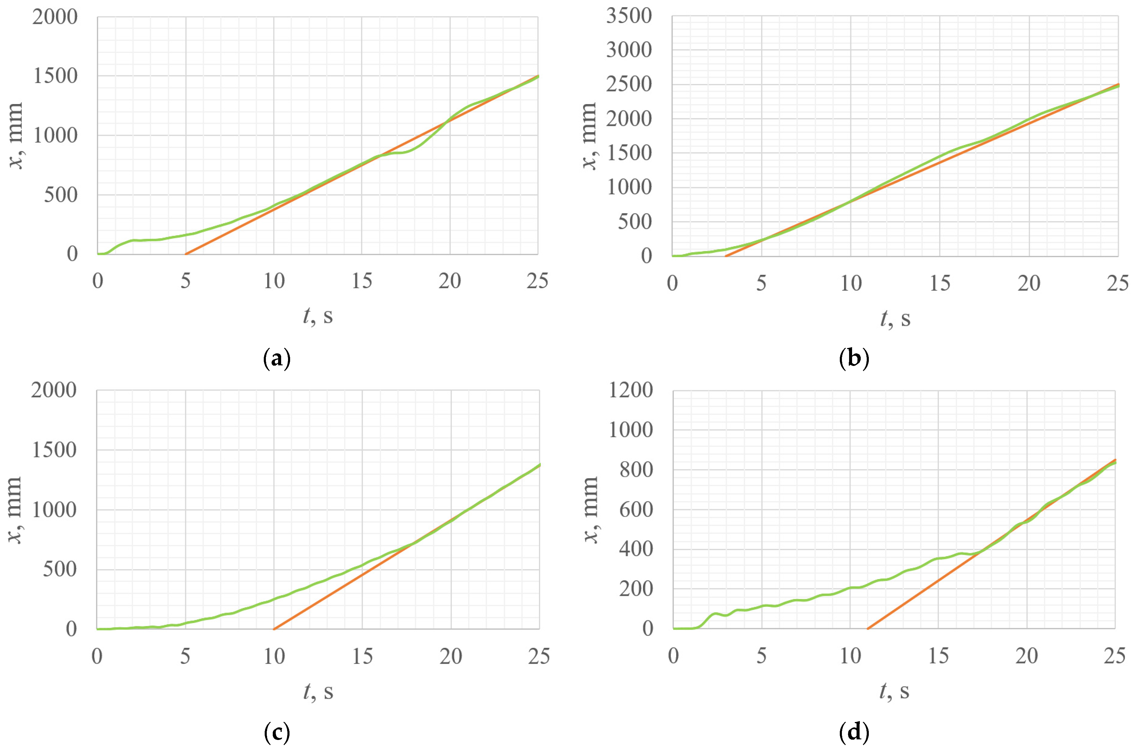
Figure 15 shows graphs of the dependence of the horizontal displacement of the extreme right upper point of the plate x at time t, determined from the results of numerical simulation, for the calculation cases: λ/L = 0.25, λ/L = 0.75, λ/L = 1.5, and λ/L = 3.0.

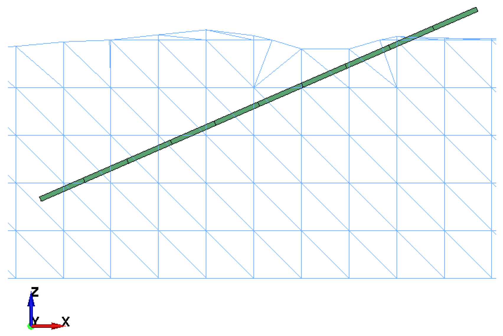
It was not possible to implement clockwise rotation of the board in the numerical model with λ/L = 1.0, since when a thin rigid body interacts with water, using the Euler–Lagrange approach, with sufficiently large dimensions of the finite elements of water and air, these elements partially «pass through» the rigid body, preventing the plate from turning (Figure 16). This drawback can be corrected by reducing the size of the water and air finite elements to approximately half the thickness of the plate (i.e., to 0.005 m), However, this solution would require a significant increase in the time required to solve the problem (up to 500–1000 h of real time for 25 s of numerical calculation, depending on the size of the model), so this option was excluded during the development of the model.

Nevertheless, due to this technical shortcoming, the plate still rotates and is flooded, but not clockwise, but counterclockwise (Figure 17), thanks to which in the numerical model at λ/L = 1.0, as well as in the experiment, the value of the ratio h_T/h_I turned out to be approximately 0.5, and the speed of the board, as can be seen in Figure 13, ultimately reduced to zero.

The results of numerical simulation yield the following approximate law for determining the dependence of v_i/v_w on λ/L at t_i ≪ L and t_i ≪ h_I ≪ λ:

$${\displaystyle \frac{v_i}{v_w}}=\left\{\begin{array}{c}0.167e^{-0.6(\mathsf{\lambda }/L)}, 0\le \lambda /L<0.5;\lambda /L>2.0\\ {\displaystyle \frac{19}{25}}{\displaystyle \frac{\mathsf{\lambda }/L}{\left(1-\mathsf{\lambda }/L\right)-3.7\ln \left(1-\mathsf{\lambda }/L\right)}}, 0.5\le \lambda /L<1\\ \begin{array}{c}0, \mathsf{\lambda }/L=1\\ {\displaystyle \frac{6}{25}}{\displaystyle \frac{\mathsf{\lambda }/L}{10\left(\mathsf{\lambda }/L-1\right)-3.7\ln \left(\mathsf{\lambda }/L-1\right)}}, 1.0<\mathsf{\lambda }/L\le 2.0\end{array}\end{array}\right.$$

(35)

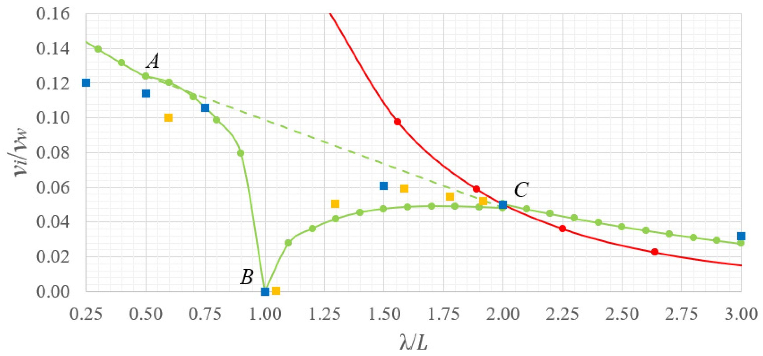
Figure 18 shows a comparison of the values of v_i/v_w = f(λ/L) obtained from (34) and (35), and the results of physical and numerical modeling. A comparison of the current and previous results is shown in a single figure, as this is the most straightforward way to directly assess the differences and similarities between the two calculation methods.

As can be seen, the ratios (35) describe the dependence of v_i/v_w on λ/L quite accurately. In addition, both the left and right parts of the graphs obtained from (35) can be connected by an approximating curve showing the theoretical value of v_i/v_w in the case where the plate did not rotate. The value of v_i/v_w at λ/L = 1.0 without taking into account the flooding of the plate in Figure 18 is approximately 0.1, which corresponds to the ratio of the speed of the plate to its overturning (according to the purple line in Figure 13, v_i = 127 mm/s) to the wave velocity at λ = 1 m and T = 0.8 s (according to Table 4, v_w = 1250 mm/s), i.e., v_i/v_w = 127/1250 $\approx$ 0.1.

The same logic applies to all values of v_i/v_w for the range λ/L = 0.5…2.0, which is described by the curved triangle ABC in Figure 18. It was not possible to establish the exact boundaries of the ABC triangle, since the numerical model proposed in this work, due to the shortcomings of the technology for implementing the interaction of finite elements of water with finite elements of a rigid body, does not accurately describe the oscillations of an ice floe on a wave surface. Based on this, expressions (35) in this work serve solely as a tool to illustrate the possible form of reduction v_i/v_w for the range of values λ/L = 0.5…2.0.

It should be noted that such behavior of a freely floating plate under the action of waves is possible only when the wave height significantly exceeds the thickness of the plate. However, if the wave height is several times greater than the thickness of the ice, the ice floe will break into smaller pieces due to its low flexural strength. Consequently, the ratio v_i/v_w can be determined only using the first expression in (35), which does not account for significant submersion of the plate at λ/L = 0.5…2.0:

$${\displaystyle \frac{v_i}{v_w}}=0.167e^{-0.6(\lambda /L)}$$

(36)

The ratios of the initial ice floe velocity to the wave front velocity for the range λ/L = 0.5…2.0 will most likely be located near the dotted green line. It is also important to note that as the ice floe begins to oscillate more strongly, its velocity will begin to decrease, which will lead to a decrease in the value of v_i/v_w, and the rate of this decrease will depend on how close the value of λ/L is to 1.0.

It can be assumed that as λ/L approaches 0, the value of v_i/v_w will tend towards 1.0, which is also not described by expressions (35), since this sharp upward turn in the graph will only be true for very small values of λ/L, because as λ decreases, the waves on the water surface will take the form of a steady current, and the plate will begin to move at the speed of this current.

When λ/L tends to infinity, the value v_i/v_w will tend to 0, since with very long waves the shape of the wave surface becomes almost flat, due to which the speed of the ice floe compared to the speed of the waves will also be insignificant.

As suggested earlier, empirical Formula (34), according to Figure 18, is indeed best suited for cases where λ/L ≥ 2.0, since for values of λ/L < 2.0, the graph of the dependence of v_i/v_w on λ/L shoots upward, taking values that do not correspond to the observed measurements.

Experimental data from [5,6,7,14,15] are used to validate the derived Formula (36).

In [5], rigid polyethylene plates of oval and square shapes were used as ice floes. The data used are results for square plates (200 × 200 mm) of two different thicknesses (30 mm and 45 mm) with $\mathsf{\rho }$_i = 960 kg/m³ and d = 0.8 m (10 data sets). In [6], the data from [4] were extended, this time for rectangular wooden plates of three different thicknesses (12 mm, 36 mm, 60 mm) at constant values of $\mathsf{\rho }$_i = 720 kg/m³, d = 0.8 m, and L = 1.2 m (102 data sets). In [7], for constant values of $\mathsf{\rho }$_i = 890 kg/m³ and d = 0.9 m, the variation in the drift velocity of rigid plates made of paraffin, of various shapes and sizes, under the influence of regular surface gravity waves was investigated. The data used were results for plates 0.3 m and 0.2 m long with a constant thickness of 0.05 m (51 data sets). In [14], at a constant water depth d = 3.5 m, plates made of wax with a density of $\mathsf{\rho }$_i = 903 kg/m³ and square, circular, and triangular shapes were used as ice floes interacting with waves. The data for this study were taken from the drift results of square plates with dimensions L = 0.6 m and t_i = 9 cm; L = 0.5 m and t_i = 9 cm; L = 0.45 m and t_i = 9 cm; L = 0.6 m and t_i = 5 cm (24 data sets). In [15], plates made of low-density polyethylene ($\mathsf{\rho }$_i = 920 kg/m³) with a length of 0.38 m and a thickness of 0.012 m were used as ice floes (27 data sets). In total, there are 214 data sets.

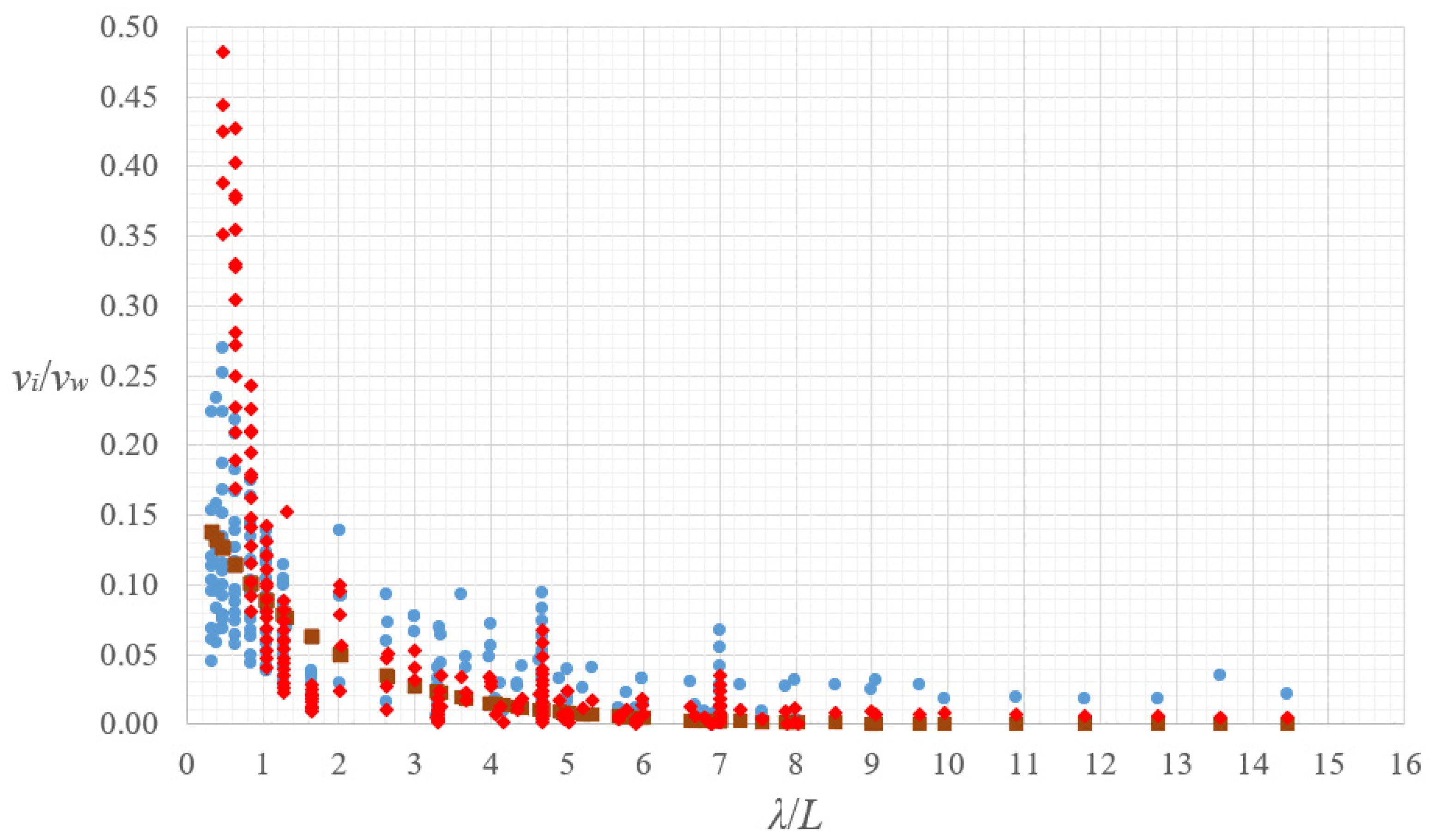
Figure 19 presents a comparison of the v_i/v_w values from [5,6,7,14,15], as well as the calculated v_i/v_w values based on the original data from [5,6,7,14,15] using Formulas (34) and (36). In this case, Formula (36) is used rather than (35) because, according to the data from [5,6,7,14,15], during wave interaction with free-floating plates, no significant submergence of the plates was observed in these studies, since the wave steepness in the studies [5,6,7,14,15] was sufficiently small: h_I/λ = 0.01…0.09.

The accuracy of the formulas is compared for two ranges: λ/L ≤ 2.0 and λ/L > 2.0. The comparison is performed by calculating the coefficient of determination R²:

$$R^2=1-{\displaystyle \frac{\sum _{j=1}^J{\left(O_j-P_j\right)}^2}{\sum _{j=1}^J{\left(O_j-{\overline{O}}_j\right)}^2}}$$

(37)

where O_j denotes the v_i/v_w values from references [5,6,7,14,15]; P_j—calculated values of v_i/v_w; J—total number of v_i/v_w values (J = 214); ${\overline{O}}_j$—arithmetic mean of v_i/v_w from [5,6,7,14,15], calculated as

$${\overline{O}}_j={\displaystyle \frac{1}{J}}{\sum }_{j=1}^J{O}_j$$

(38)

The results of the R² calculations for the v_i/v_w values are presented in

Table 5. R² values obtained by comparing the observed v_i/v_w data from [5,6,7,14,15] with the calculated v_i/v_w values from Equations (34) and (36).

Formula	R2
At λ/L ≤ 2.0
(34)	−38.59
(36)	0.26
At λ/L > 2.0
(34)	0.41
(36)	−0.31

.

As can be seen, the comparison confirms the previously proposed conclusions. Equation (34) yields more accurate results for the range λ/L > 2.0, whereas for the range λ/L ≤ 2.0, more accurate values of v_i/v_w are obtained by calculating using Equation (36).

3.3. Results of Analytical Research

The parameters for calculation were taken as similar model values from the experiment. With a plate material density of ${\mathsf{\rho }}_i$ = 720 kg/m³ and dimensions L = 1 m, B = 1.14 m, t_i = 0.01 m, the plate mass M is equal to M = LBt_i${\mathsf{\rho }}_i$ =1 × 1.14 × 0.01 × 720 = 8.20 kg. The mass moment of inertia of the plate J with the same dimensions is equal to J = M(B² + t_i²)/12 = 8.20 × (1.14² + 0.01²)/12 = 0.89 kg·m². The water depth d = 0.5 m. The density of water $\mathsf{\rho }$ = 1000 kg/m³. The acceleration due to gravity g = 9.81 m/s².

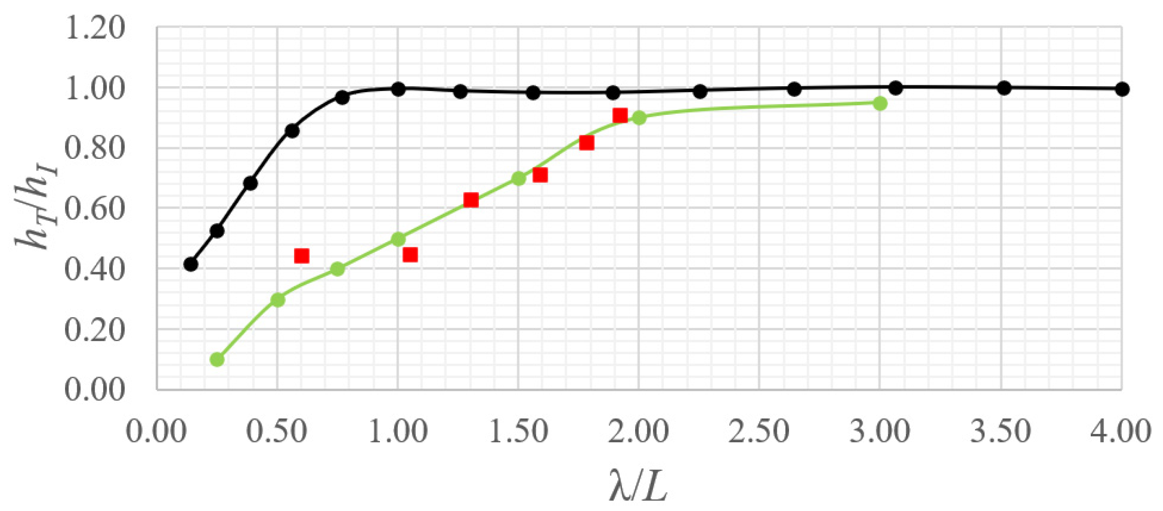
The height of the falling waves is taken to be h_I = 0.1 m. The calculation is performed for a range of wave periods T = 0.3…1.6 s with a step of 0.1 s. The wavelength λ is determined by Equation (1). The values of h_T, C_R and C_T are calculated. The calculation results are presented in

Table 6. Analytical calculation of the C_R and C_T coefficients for the task of determining h_T/h_I.

No.	T, s	λ, m	hT, m	CR	CT
1	0.30	0.14	0.05	0.91	0.42
2	0.40	0.25	0.06	0.85	0.53
3	0.50	0.39	0.08	0.73	0.69
4	0.60	0.56	0.10	0.51	0.86
5	0.70	0.77	0.11	0.24	0.97
6	0.80	1.00	0.11	0.10	0.99
7	0.90	1.26	0.11	0.16	0.99
8	1.00	1.56	0.11	0.19	0.98
9	1.10	1.89	0.11	0.18	0.98
10	1.20	2.25	0.11	0.15	0.99
11	1.30	2.64	0.11	0.09	1.00
12	1.40	3.06	0.11	0.03	1.00
13	1.50	3.51	0.11	0.05	1.00
14	1.60	4.00	0.11	0.11	0.99

.

Figure 20 shows a graph of the analytical calculation of the change in the ratio h_T/h_I as a function of λ/L, as well as the values of h_T,n/h_I,n determined during the experiment and the values of h_T/h_I found using numerical simulation.

As can be seen, the value of h_T/h_I in the analytical model becomes equal to 1.0 at λ/L = 1.0, while according to the experimental data and the numerical model, it becomes equal to 1.0 at approximately λ/L = 2.0. Up to a value of h_T/h_I = 0.5, the calculation using the analytical model decreases only at approximately λ/L = 2.0, while the results of the experiment and the numerical model show a decrease already at λ/L = 1.0.

This discrepancy can be explained by the fact that, since the mathematical model in [31] is based on the linear theory of small-amplitude waves in shallow water, two basic conditions must be satisfied to obtain adequate results: d/λ ≪ 1 and h_I/λ ≪ 1 [31]. Neither of these conditions corresponds to the initial data for the experiment and numerical simulation (since the value of d/λ ranges from 0.17 to 2.00, and the parameter h_I/λ ranges from 0.03 to 0.20).

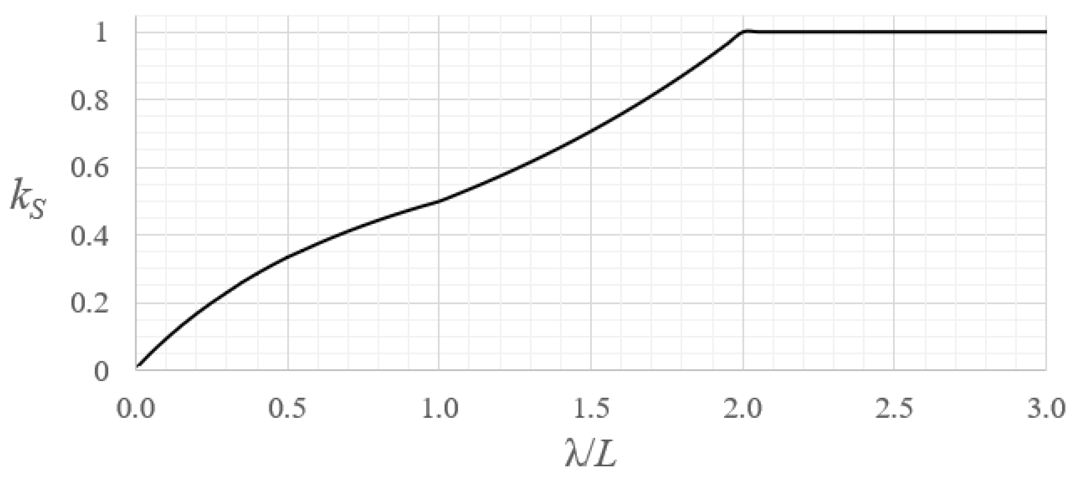
As a result, the analytical model does not take into account the separation of the plate from the water surface, since the movement of the plate itself is determined by the free wave surface equation, as a result of which partial flooding of the plate, as observed in the experiment, is impossible in the analytical model. Because of this, the model does not take into account the additional reflection of waves from the sides and bottom of the plate caused by this effect, as a result of which the model shows overestimated values of h_T/h_I depending on λ/L. To correct this, it is proposed to introduce a correction coefficient k_S for the height of the transmitted waves into the analytical model, which is defined as:

$$k_S=\left\{\begin{array}{c}{\displaystyle \frac{1}{L/\mathsf{\lambda }+1}}, \lambda /L\le 1\\ 2^{\mathsf{\lambda }/L-2}, 1<\lambda /L<2\\ 1, \lambda /L\ge 2\end{array}\right.$$

(39)

The influence of the plate thickness t_i on k_S in (39) is not taken into account, since cases of wave interaction with ice floes having dimensions t_i ≪ L and t_i ≪ h_I are considered.

The dependence of k_S on λ/L is shown in Figure 21.

The boundary values k_S = 1/(L/λ+1) at λ/L ≤ 1.0 and k_S = 1.0 at λ/L ≥ 2.0 were adopted based on the assumptions that:

(1)

The analytical model shows the correct nature of the decrease in h_T/h_I with a decrease in the value of λ/L below 1.0, but does not take into account the phase shift of the waves and ice floes when two wave crests of different amplitudes are formed under the plate, causing the plate to rotate and, as a result, partially flooding its rear edge. It can be assumed that in the case of an even greater number of complete waves fitting under the floating plate, the coefficient k_S will decrease even more and will be inversely proportional to the number of wave crests under the plate base, i.e., k_S~1/(L/λ + 1).

(2)

When interacting with waves more than twice as long as the ice floe, the plate will practically float on the wave surfaces, since it will always interact with only one of the crests of the wave front, thus avoiding the risk of capsizing and partial flooding.

The approximation formula $k_S (\mathsf{\lambda }/L)=2^{\mathsf{\lambda }/L-2}$ at 1.0 < λ/L < 2.0 was derived from the assumption that the function k_S on the interval λ/L = 1.0…2.0 can be described by the exponential law $k_S(\mathsf{\lambda }/L)=A{e}^{B\left(\mathsf{\lambda }/L-1\right)}$, which satisfies the boundary conditions at k_S(1) = 0.5 and k_S(2) = 1.0. In this case, the proposed expression at λ/L = 1.0 will give k_S(1) = A → A = 0.5, and at λ/L = 2.0: k_S(2) = $A{e}^B$ = 0.5$e^B$ = 1.0 → B = ln(2). In this case, $k_S(\lambda /L)=0.5e^{\ln \left(2\right)\left(\lambda /L-1\right)}=2^{\lambda /L-2}$ at λ/L = 1.0…2.0.

The new value of the height of the waves that have passed $h_T^{\prime }$ will then be determined by:

$$h_T^{\prime }={k_{S}h}_T$$

(40)

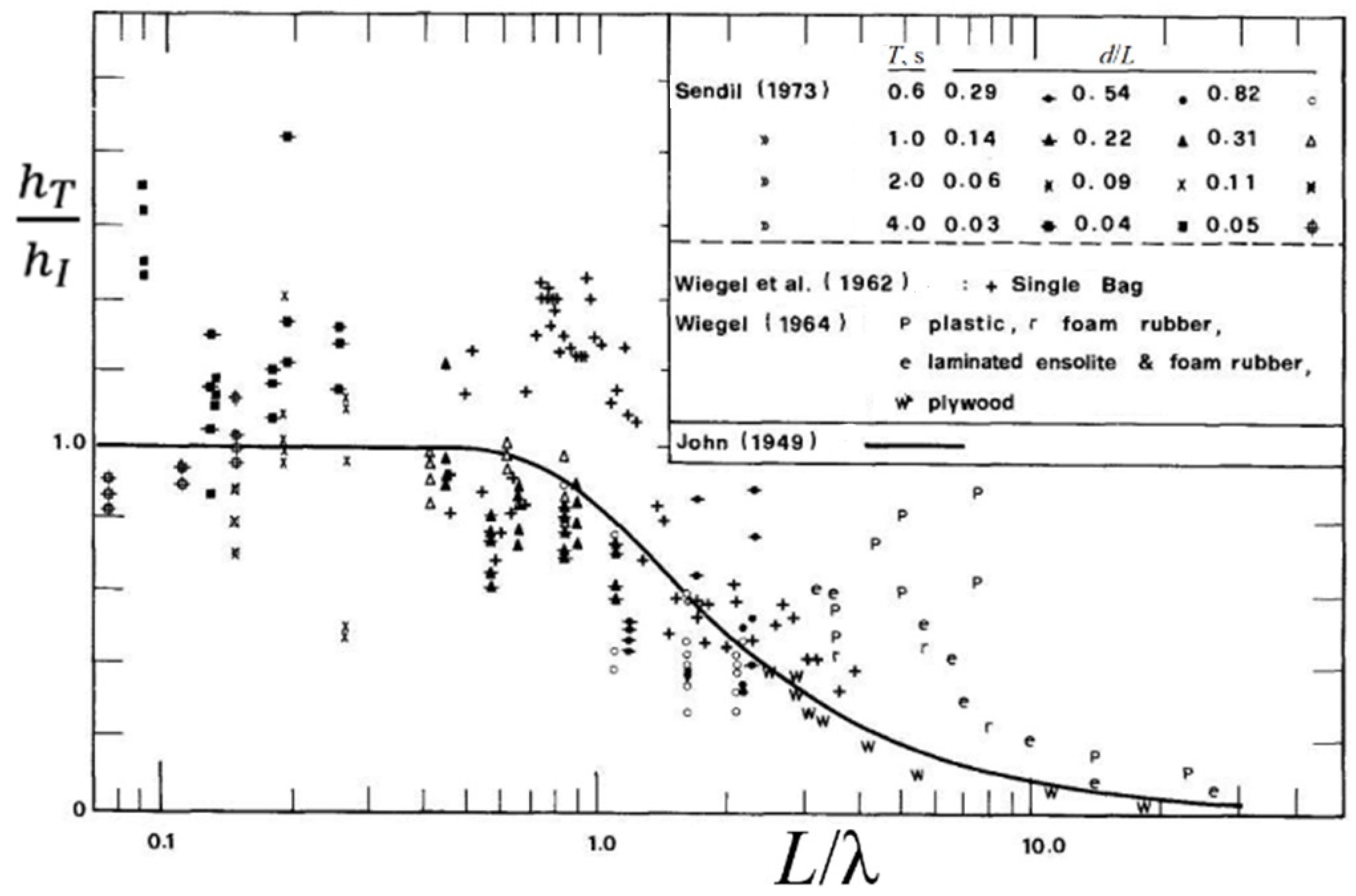
The calculation of h_T/h_I taking into account (39) for the data from Table 6 is compared with the approximate analytical formula for determining the ratio h_T/h_I from the work of F. John, 1949 [33], which was verified in the work of U. Sendil, 1974 [34], based on several laboratory experiments and comparison with the results of other studies on the interaction of waves with floating breakwaters (Figure 22):

$${\displaystyle \frac{h_T}{h_I}}=\sqrt{1-{\left\{{\displaystyle \frac{{\mathsf{\theta }}^5}{45\sqrt{\left[{\left(1-\frac{2}{5}{\mathsf{\theta }}^2\right)}^2+{\mathsf{\theta }}^2{\left(1-\frac{{\mathsf{\theta }}^2}{15}\right)}^2\right]\left[{\left(1-\frac{{\mathsf{\theta }}^2}{3}\right)}^2+{\mathsf{\theta }}^2\right]}}}\right\}}^2},$$

(41)

where θ = πL/λ.

In addition, as indicated in the work of R.R. Rumer, 1979 [37], devoted to the study of the interaction of waves, wind, and freely drifting ice floes, Formula (41) can be used to calculate the change in wave amplitude when waves pass through freely floating ice floes.

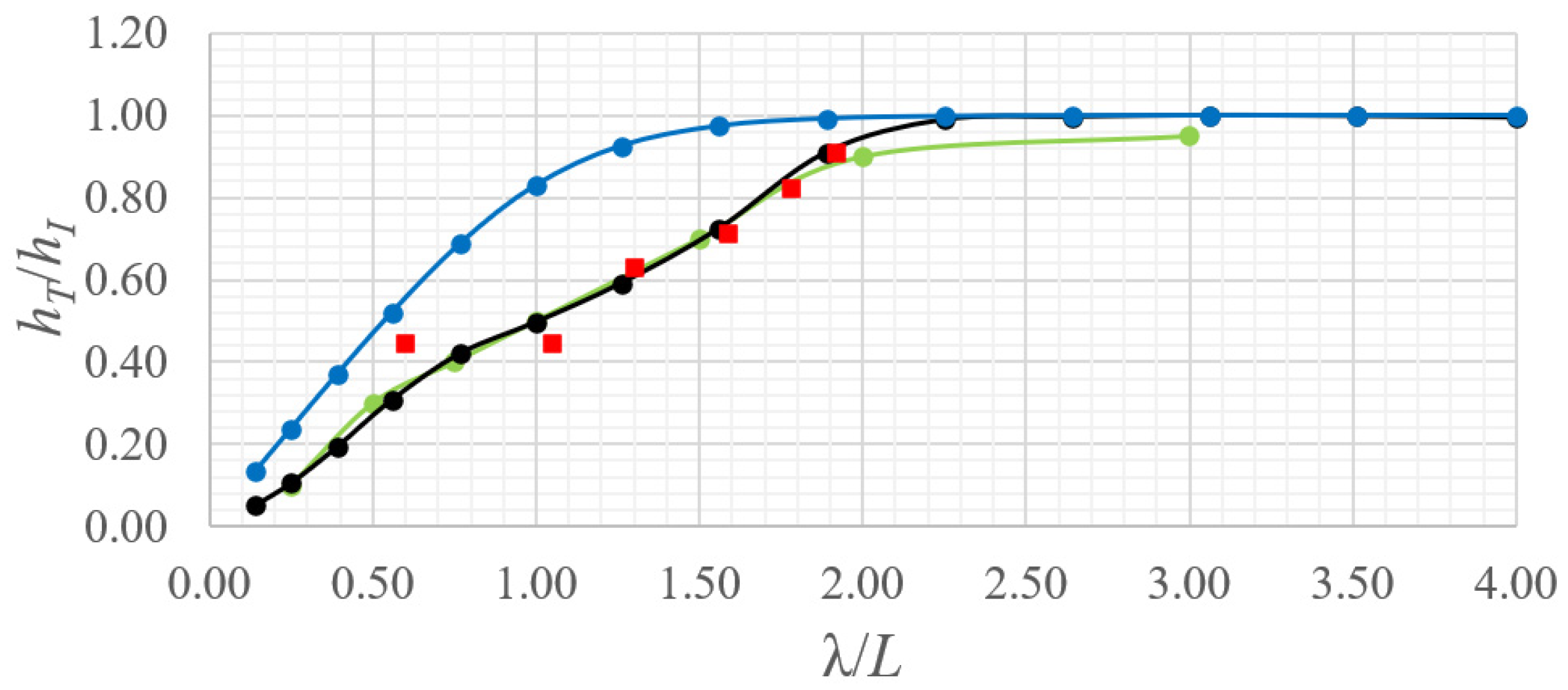
Figure 23 shows a comparison of the graph of the change in h_T/h_I as a function of λ/L, taking into account the application of the coefficient k_S, the calculation of h_T/h_I made using Formula (41), and the values of h_T/h_I obtained from the results of physical and numerical simulations within the framework of this work.

As can be seen in Figure 23, the analytical model now gives results close to those obtained in the experiment and numerical modeling. However, the calculation using Formula (41) does not coincide with the results of the analytical model. This is due to the fact that Formula (41) was calculated analytically for the case of an infinitely small coefficient of settlement of a rectangular body [33], which is why it takes into account wave attenuation but does not take into account the effect of plate flooding.

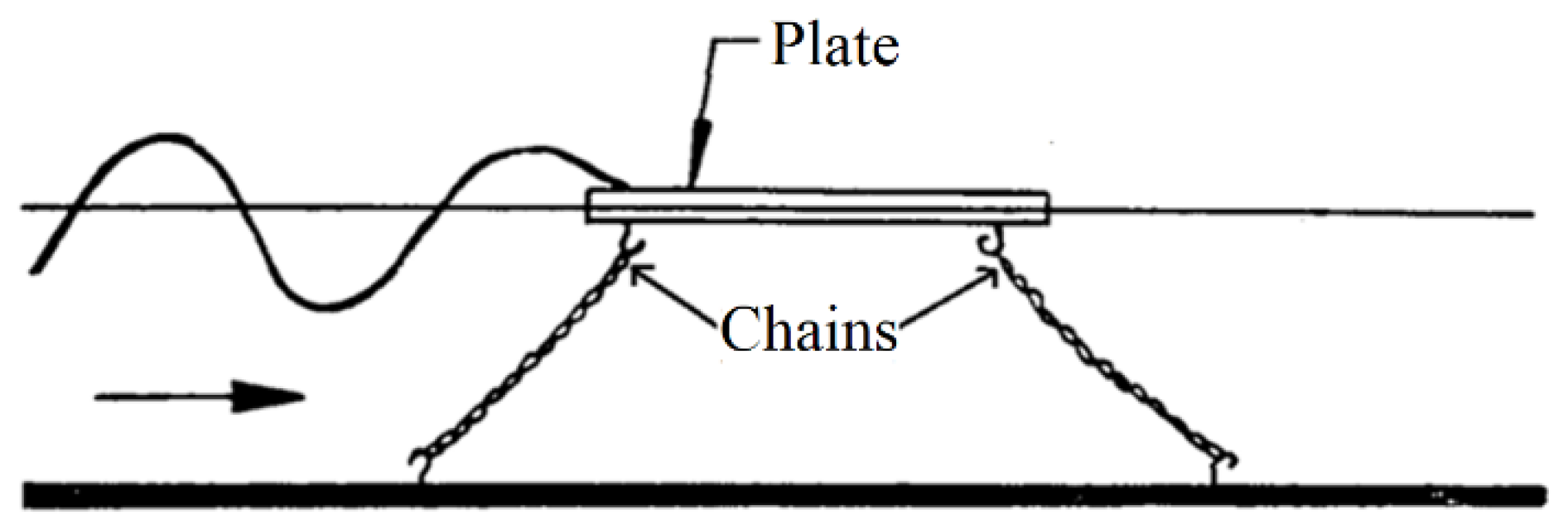
In addition, in the work of U. Sendil, 1973 [35], in Figure 22, Formula (41) was verified for cases of wave interaction with a body whose attachment to the bottom was provided by light chains and hooks (Figure 24). As a result, during the experiments, the floating body was restricted in both horizontal and vertical movements, so that during the experiments there was no significant flooding of the plate at λ/L = 1.0. The same applies to the work of R.L. Wiegel, 1962 [36], where water cushions were used as breakwaters, which were also attached to the sides of the laboratory pool with mooring ropes.

Thus, it can be concluded that the analytical model developed in this work can be used to determine the change in wave height as they pass through free-floating ice floes for conditions satisfying a small relative thickness of the ice floe (compared to the wave height) and the application of linear wave theory. The assumption made in [37] that Formula (41) is suitable for determining the wave transmission coefficient through drifting ice floes proved to be insufficiently correct.

Formula (41) can be used when h_I ≪ λ and t_i ≪ L for cases t_i ≫ h_I, since under such conditions there will be no partial flooding of the plate, while the analytical model developed in this study is suitable for cases t_i ≪ h_I, in which the effect of ice flooding is most likely to occur. Accordingly, it can be assumed that the values of h_T/h_I obtained for the remaining variants of the relationships between t_i and h_I will fall within the range of values obtained using these two calculation methods.

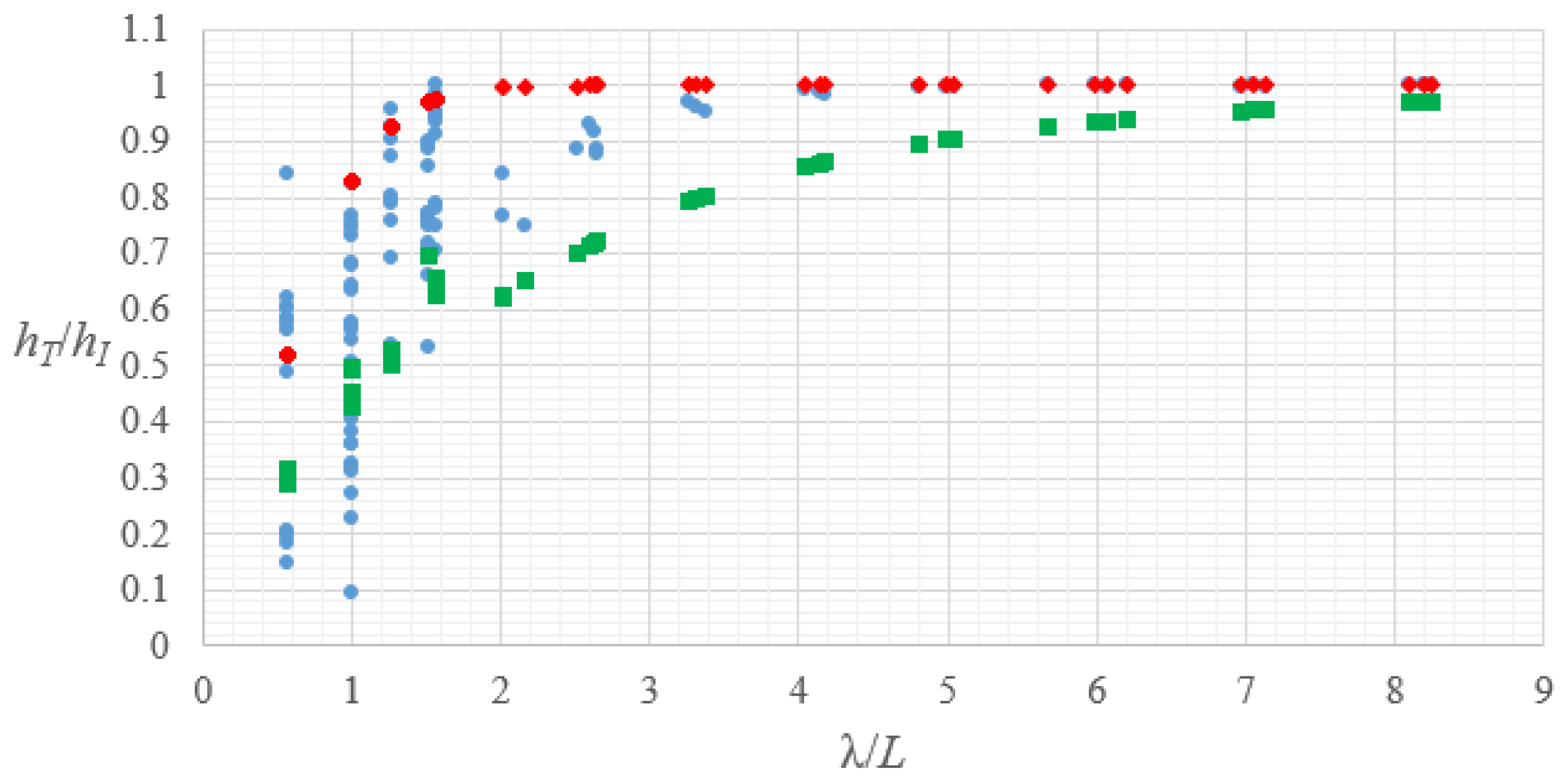
Experimental data from [8,10,11,12,15] are used to validate the developed mathematical model.

In [8], ice floes were represented by plates 1 m long and 5 mm, 10 mm, and 20 mm thick, made of polyvinyl chloride (ρ_i = 500 kg/m³) and polypropylene (ρ_i = 905 kg/m³); however, this study uses data only for polypropylene plates (36 data sets). In [10], wave reflection from floating breakwaters with a rectangular cross-section (L = 1 m, t_i = 10 mm) made of polyvinyl chloride (ρ_i = 569 kg/m³) and polypropylene (ρ_i = 905 kg/m³), both moored to the seabed and freely floating under the action of waves. This study includes results corresponding to the case of a freely floating plate with a density of 905 kg/m³ (15 data sets). In [11], a rectangular polypropylene plate with the following physical and geometric characteristics was used as the freely floating plate: ρ_i = 905 kg/m³, L = 1 m, and t_i = 10 mm (18 data sets). In [12], a square plate 1 m long and 5 mm thick, made of polypropylene with a density of ρ_i = 905 kg/m³, was used as an ice floe (6 data sets). From [14], the same results used to determine the ice floe drift velocity were taken as data (27 data sets). In total, there are 102 data sets.

In the accepted initial data from [8,10,11,12,15], the range of d/λ values is 0.33…1.97 (which is comparable to the d/λ values in the physical and numerical models), and the wave steepness ranges from h_I/λ = 0.006 to h_I/λ = 0.073 (which are, on average, smaller than the wave steepness in the physical and numerical models). Figure 25 presents a comparison of the values of h_T/h_I from [8,10,11,12,15], as well as the calculated values of h_T/h_I based on the initial data from [8,10,11,12,15] using Formula (41) and based on the developed mathematical model, taking into account the inundation coefficient k_s.

As can be seen, Equation (41) roughly describes the upper limit of the data from [8,10,11,12,15] (since it does not account for ice floe submersion), whereas the results of the mathematical model correspond to the lower limit of the data from [8,10,11,12,15] (since it accounts for maximum ice submersion). Thus, it is assumed that the developed mathematical model forms an approximate range of minimum values for h_T/h_I as the values of h_I/λ and h_I/t_i approach infinity.

The only deviation of the observed data from the predicted values is observed at λ/L = 1.0, which is most likely due to the occurrence of a resonance effect between the waves and the ice floe, which is not accounted for in Equation (41) or in the determination of the submergence coefficient k_s using expression (39).

4. Conclusions

• To ensure the safety and reliability of hydraulic structures under wave and ice loads, it is necessary to know the ice drift velocity toward the structure, as well as how free-floating ice floes dissipate wave energy, thereby reducing the height of the passing waves. Currently, there are no adequate analytical models that allow these quantities to be reliably determined. Existing analytical formulas for calculating ice drift velocity are applicable mainly to cases where the wavelength is more than twice the horizontal dimensions of the ice floe. In turn, existing analytical formulas for calculating the wave transmission coefficient through a free-floating ice floe do not account for wave overwash, as well as the submersion of the ice floe, as a result of which they overestimate the height of the transmitted waves.
• To address the above-mentioned shortcomings, this article presents physical and numerical modeling, as well as analytical studies of the interaction of surface waves with a free-floating plate simulating an ice floe. The laboratory experiment involved the interaction of waves generated in a hydraulic flume with a freely floating wooden plate; all similarity criteria were satisfied. For numerical modeling, the LS-DYNA R11.0 software package was used, in which water was modeled using the Euler–Lagrange method, and the ice floe was modeled as a freely floating elastic–plastic plate. In the mathematical model, the linear theory of waves in shallow water was applied, where the free-surface function was used instead of the bending deformation equation for an elastic plate; to account for the effect of plate submergence, an empirical submergence coefficient was introduced into the analysis. The same initial data were used for all three models.
• Physical and numerical simulations have shown that, for sufficiently steep waves whose height exceeds the thickness of the ice plate, a sharp decrease in the ice floe’s velocity is observed in the range λ/L = 0.5…2.0, dropping to zero at λ/L = 1.0. This is explained by the resonance that arises between the motion phases of the ice floe and the wave when the horizontal dimensions of the plate coincide with the wavelength.
• Based on the results of physical and numerical modeling, an empirical formula was derived to determine the ice drift velocity. The results obtained using this formula were compared with calculations based on existing similar formulas, where the results of other studies were used as input and observed data. The comparison showed that the proposed formula yields more accurate results in cases where the wavelength does not exceed twice the horizontal dimensions of the ice plate.
• Based on the results of the mathematical model, supplemented by the submergence coefficient, the lower limit of the wave transmission coefficient through a freely floating plate was determined as a function of λ/L for cases involving steep waves whose height significantly exceeds the plate thickness.

To further develop this topic, it is necessary to continue studying the influence of water depth, wave height, and plate thickness on the drift velocity of the ice floe and the wave transmission coefficient. To this end, more experimental studies and numerical simulations of wave–ice interaction should be conducted, especially for cases where the wavelength does not exceed twice the horizontal dimensions of the ice floe. In the future, once a sufficient amount of data has been accumulated, it will be advisable to apply machine learning methods to solve this problem.

References

1. Code of Rules 38.13330.2018; Loads and Impacts on Hydraulic Structures (Wave, Ice and from Ships). Standartinform Publ.: Moskow, Russia, 2018. (In Russian)
2. El-Tahan, M.S.; EI-Tahan, H.W.; Venkatesh, S. Forecast of iceberg ensemble drift. In Proceedings of the 15th Annual Offshore Technology Conference, Houston, TX, USA, 2–5 May 1983; pp. 151–158. [Google Scholar] [CrossRef]
3. Wadhams, P.; Kristensen, M.; Orheim, O. The response of Antarctic icebergs to ocean waves. J. Geophys. Res. Oceans 1983, 88, 6053–6065. [Google Scholar] [CrossRef]
4. Arikainen, A.I. Wave drift of an isolated floe. AIDJEX Bull. 1972, 16, 125–131. [Google Scholar]
5. Huang, G.; Law, A.W.K.; Huang, Z. Wave-induced drift of small floating objects in regular waves. Ocean Eng. 2011, 38, 712–718. [Google Scholar] [CrossRef]
6. Huang, G.; Law, A.W.K. Wave-induced Drift of Large Floating Objects in Regular Waves. J. Waterw. Port Coast. Ocean Eng. 2013, 139, 535–542. [Google Scholar] [CrossRef]
7. McGovern, D.J.; Bai, W. Experimental study on kinematics of sea ice floes in regular waves. Cold Reg. Sci. Technol. 2014, 103, 15–30. [Google Scholar] [CrossRef]
8. Bennetts, L.G.; Alberello, A.; Meylan, M.H.; Cavaliere, C.; Babanin, A.V.; Toffoli, A. An idealised experimental model of ocean surface wave transmission by an ice floe. Ocean Model 2015, 96, 85–92. [Google Scholar] [CrossRef]
9. He, M.; Ren, B.; Qiu, D. Experimental study of nonlinear behaviors of a free-floating body in waves. China Ocean Eng. 2016, 30, 421–430. [Google Scholar] [CrossRef]
10. Nelli, F.; Bennetts, L.G.; Skene, D.M.; Monty, J.P.; Lee, J.H.; Meylan, M.H.; Toffoli, A. Reflection and transmission of regular water waves by a thin, floating plate. Wave Motion 2017, 70, 209–221. [Google Scholar] [CrossRef]
11. Toffoli, A.; Bennetts, L.G.; Meylan, M.H.; Cavaliere, C.; Alberello, A.; Elsnab, J.; Monty, J.P. Sea ice floes dissipate the energy of steep ocean waves. Geophys. Res. Lett. 2015, 42, 8547–8554. [Google Scholar] [CrossRef]
12. Toffoli, A.; Pitt, J.P.A.; Alberello, A.; Bennetts, L.G. Modelling attenuation of irregular wave fields by artificial ice floes in the laboratory. Phil. Trans. A Math. Phys. Eng. Sci. 2022, 380, 20210255. [Google Scholar] [CrossRef]
13. Li, H.; Lubbad, R. Laboratory Study of Ice Floes Collisions under Wave Action. In Proceedings of the 28th International Ocean and Polar Engineering Conference, Sapporo, Japan, 10–15 June 2018; pp. 1516–1524. [Google Scholar]
14. Wang, C.; Song, M.; Guo, C.; Wang, S.; Tian, T.; Luo, W. Experimental Study of Sea Ice Motion in Waves. J. Cold Reg. Eng. 2020, 34, 04020010. [Google Scholar] [CrossRef]
15. Park, S.B.; Shin, S.Y.; Shin, D.G.; Park, H.; Jung, K.H.; Suh, S.B.; Lee, J.; Lee, S.J.; Kim, H.S. Experimental study of wave transmission and drift velocity using freely floating synthetic ice floes. Ocean Eng. 2022, 251, 111058. [Google Scholar] [CrossRef]
16. Tavakoli, S.; Huang, L.; Azhari, F.; Babanin, A.V. Viscoelastic Wave-Ice Interactions: A Computational Fluid-Solid Dynamic Approach. J. Mar. Sci. Eng. 2022, 10, 1220. [Google Scholar] [CrossRef]
17. Zha, R.; Zhao, W.; Wan, D. Numerical study of wave-ice floe interactions and overwash by a meshfree particle method. Ocean Eng. 2023, 286, 115681. [Google Scholar] [CrossRef]
18. Yu, C.; Tian, Y. Numerical Simulation of Regular Wave and Ice Floe Interaction Using Coupled Eulerian–Lagrangian Method. Water 2025, 17, 1879. [Google Scholar] [CrossRef]
19. Lopatukhin, L.I.; Buhanovskij, A.B.; Degtyarev, A.B.; Rozhkov, V.A. Reference Data of Wind and Waves Climate of the Barents, Okhotsk, and Caspian Seas; Russian Maritime Register of Shipping: Saint-Petersburg, Russia, 2003. (In Russian) [Google Scholar]
20. Terziev, F.S.; Girdyuk, G.V.; Zykova, G.G.; Dzhenyuk, S.L. Hydrometeorology and Hydrochemistry of the USSR Seas; Vol. 1. Barents Sea. Issue 1. Hydrometeorological Conditions; Gidrometeoizdat: Leningrad, Russia, 1990. (In Russian) [Google Scholar]
21. Barenblatt, G.I. Scaling, Self-Similarity, and Intermediate Asymptotics; Cambridge University Press: Cambridge, UK, 1996. [Google Scholar]
22. Lighthill, M.J. Waves in Fluids; Cambridge University Press: Cambridge, UK, 1978. [Google Scholar]
23. Timco, G.W.; Weeks, W.F. A review of the engineering properties of sea ice. Cold Reg. Sci. Technol. 2010, 60, 107–129. [Google Scholar] [CrossRef]
24. Korzhavin, K.N. Action of Ice on Engineering Structures; Publishing House of Siberian Branch of USSR Academy of Sciences: Novosibirsk, Russia, 1962. (In Russian) [Google Scholar]
25. Xu, J.; Wang, J.; Souli, M. SPH and ALE formulations for sloshing tank analysis. Int. J. Multiphys. 2015, 9, 209–224. [Google Scholar] [CrossRef]
26. Varas, D.; Zaera, R.; Lopez-Puente, J. Numerical modelling of the hydrodynamic ram phenomenon. Int. J. Impact Eng. 2009, 36, 363–374. [Google Scholar] [CrossRef]
27. Cai, Z.; Topa, A.; Djukic, L.; Herath, M.T.; Pearce, G.M.K. Evaluation of rigid body force in liquid sloshing problems of a partially filled tank: Traditional CFD/SPH/ALE comparative study. Ocean Eng. 2021, 236, 109556. [Google Scholar] [CrossRef]
28. Behnen, J. Simulation of Wave-Ice-Structure Interaction. Master Thesis, Hamburg University of Technology, Hamburg, Germany, 28 July 2021. [Google Scholar]
29. Kantarzhi, I.G.; Afonyushkin, M.S. Numerical modeling of wave-ice interaction with a single support. Int. J. Comput. Civ. Struct. Eng. 2024, 20, 31–42. [Google Scholar] [CrossRef]
30. Afonyushkin, M.S.; Kantarzhi, I.G. Joint impact of waves and ice on the structure during ice breakup. Proc. VNIIG 2025, 315, 3–14. (In Russian) [Google Scholar]
31. Stoker, J.J.; Fleishman, B.; Weliczker, W.L. Floating Breakwaters in Shallow Water; Courant Institute of Mathematical Sciences, New York University: New York, NY, USA, 1953. [Google Scholar]
32. Harms, V.W. Steady Wave-Drift of Modeled Ice Floes. J. Waterw. Port Coast. Ocean Eng. 1987, 113, 606–622. [Google Scholar] [CrossRef]
33. John, F. On the Motion of Floating Bodies. I. Commun. Pure Appl. Math. 1949, 2, 13–57. [Google Scholar] [CrossRef]
34. Sendil, U.; Graf, W.H. Transmission of Regular Waves Past Floating Plates. In Proceedings of the 14th International Conference on Coastal Engineering, Copenhagen, Denmark, 24–28 June 1974; pp. 1924–1936. [Google Scholar] [CrossRef]
35. Sendil, U. Transmission of Water Waves Past Horizontal Plates. Ph.D. Thesis, Lehigh University, Bethlehem, PA, USA, 26 June 1973. [Google Scholar]
36. Wiegel, R.L.; Shen, H.W.; Cumming, J.D. Final Report on Hovering Breakwater; University of California, Hydraulic Engineering Laboratory, Wave Research Projects: Oakland, CA, USA, 1962. [Google Scholar]
37. Rumer, R.R.; Crissman, R.D.; Wake, A. Ice Transport in Great Lakes; Great Lakes Environmental Research Laboratory, National Oceanic and Atmospheric Administration, U.S. Department of Commerce: Ann Arbor, MI, USA, 1979.
Figure 1. Grid for measuring horizontal plate movements.
Water 18 01091 g001
Figure 2. Wave damper with steel filings at the rear of the flume.
Water 18 01091 g002
Figure 3. Image of the physical model for the task of determining the horizontal displacements of the plate and changes in wave amplitude as waves pass through a freely floating plate. Dimensions are given in mm.
Water 18 01091 g003
Figure 4. Operation of the physical model for the task of determining the plate’s displacements and the amplitudes of: (a) incident waves; (b) transmitted waves. Dimensions are given in mm.
Water 18 01091 g004
Figure 5. Ice size distribution function f for the Barents Sea: 1—width B; 2—length L [20].
Water 18 01091 g005
Figure 6. Numerical model of wave–ice interaction in the LS-DYNA code.
Water 18 01091 g006
Figure 7. Change in water level at T n λ / L = 0.5 = 7   s : (a) before the waves pass through the plate; (b) after the waves pass through the plate.
Water 18 01091 g007
Figure 8. Change in water level at T n λ / L = 1.0 = 9   s : (a) before the waves pass through the plate; (b) after the waves pass through the plate.
Water 18 01091 g008
Figure 9. Change in water level at T n λ / L = 2.0 = 13   s : (a) before the waves pass through the plate; (b) after the waves pass through the plate.
Water 18 01091 g009
Figure 10. The lengths of the waves obtained in the experiment: (a) at T m λ / L = 0.5 = 0.63   s ; (b) at T m λ / L = 1.0 = 0.81   s ; (c) at T m λ / L = 2.0 = 1.18   s .
Water 18 01091 g010
Figure 11. Partial flooding of the plate: (a) at λ/L = 1.0; (b) at λ/L = 0.5.
Water 18 01091 g011
Figure 12. Dependence of x on t at λ/L = 0.5 for physical and numerical models: blue line—results for the physical model; green line—results for the numerical model; orange line—linearized velocity of steady motion of the plate (vi = 95 mm/s).
Water 18 01091 g012
Figure 13. Dependence of x on t at λ/L = 1.0 for physical and numerical models: blue line—results for the physical model; green line—results for the numerical model; orange line—linearized velocity of steady motion of the plate (vi = 0); purple line—linearized velocity of the plate before the start of its rotation (vi = 127 mm/s).
Water 18 01091 g013
Figure 14. Dependence of x on t at λ/L = 2.0 for physical and numerical models: blue line—results for the physical model; green line—results for the numerical model; orange line—linearized velocity of steady motion of the plate (vi = 84 mm/s).
Water 18 01091 g014
Figure 15. The dependence of x on t obtained from the results of numerical modeling (green line) and the linearized velocity of the steady motion of the plate (orange line): (a) at λ/L = 0.25 (vi = 75 mm/s); (b) at λ/L = 0.75 (vi = 114 mm/s); (c) at λ/L = 1.5 (vi = 91 mm/s); (d) at λ/L = 3.0 (vi = 61 mm/s).
Water 18 01091 g015
Figure 16. The difference in the forms of interaction between water and a rigid body at λ/L = 1.0: (a) in the physical model; (b) in the numerical model.
Water 18 01091 g016
Figure 17. Counterclockwise rotation of the plate in the numerical model at λ/L = 1.0.
Water 18 01091 g017
Figure 18. Dependence of vi/vw versus λ/L: red line—calculation according to (34); green solid line—calculation according to (35); green dotted line—connecting section describing the theoretical absence of strong plate rotation at λ/L = 0.5…2.0; blue squares—numerical simulation results; orange squares—physical simulation results.
Water 18 01091 g018
Figure 19. Dependence of vi/vw on λ/L: blue circles—data from [5,6,7,14,15]; red diamonds—calculation using Equation (34); brown squares—calculation using Equation (36).
Water 18 01091 g019
Figure 20. Change in hT/hI depending on the ratio λ/L: black line—results of analytical calculation; green line—results of numerical simulation; red squares—results of the experiment.
Water 18 01091 g020
Figure 21. The dependence of kS on λ/L.
Water 18 01091 g021
Figure 22. Dependence of hT/hI on L/λ [34]. The data is taken from [33,35,36].
Water 18 01091 g022
Figure 23. Change in hT/hI as a function of the ratio λ/L: black line—results of analytical calculation taking into account the application of the submergence coefficient kS; green line—results of numerical modeling; blue line—calculation using Formula (38); red squares—experimental results.
Water 18 01091 g023
Figure 24. Schematic diagram of the interaction between waves and a floating breakwater [35].
Water 18 01091 g024
Figure 25. Dependence of hT/hI on λ/L: blue circles—data from [8,10,11,12,15]; red diamonds—calculation using Equation (41); green squares—calculation using the developed mathematical model, taking into account the submergence coefficient ks.
Water 18 01091 g025