Article

Forecasting Suspended Sediment Concentration and Sediment Flux in the Lower Mekong Delta Using Machine Learning

1
Water Resources Engineering Faculty, College of Engineering, Can Tho University, Can Tho 900000, Vietnam
2
Land Resources Department, College of Environment and Natural Resources, Can Tho University, Can Tho 900000, Vietnam
3
Water Resources Department, College of Environment and Natural Resources, Can Tho University, Can Tho 900000, Vietnam
4
Institute for Global Environmental Strategies, Hayama 240-0115, Japan
*
Author to whom correspondence should be addressed.
Water 2026, 18(8), 923; https://doi.org/10.3390/w18080923
Submission received: 2 March 2026 / Revised: 27 March 2026 / Accepted: 9 April 2026 / Published: 13 April 2026
(This article belongs to the Special Issue Soil Erosion and Sedimentation by Water)

Abstract

Suspended sediment concentration (SSC) and sediment flux (SF) are critical indicators of sediment delivery in the Lower Mekong and underpin deltaic geomorphic stability and ecosystem services. With recent evidence of declining sediment supply caused by upstream regulation and intensive in-channel extraction, there is a pressing need for data-efficient tools to reproduce non-linear sediment dynamics and assist management in the Vietnamese Mekong Delta (VMD). This study evaluates three machine-learning algorithms—Random Forest (RF), Support Vector Machine (SVM), and Extreme Gradient Boosting (XGBoost)—for data-driven prediction of SSC (2009–2023) and SF (2009–2021) at Tan Chau (Viet Nam). The predictive models were developed using daily discharge inputs from Kratie (Cambodia) and local hydrological data, including water levels and discharge, from the Tan Chau station. Across the held-out testing dataset, all models captured substantial variability in both targets, with consistently higher performance for SF than for SSC. RF achieved the highest skill (SSC: R2 = 0.783; SF: R2 = 0.867), followed by XGBoost and then SVM. Variable-importance analysis indicates that upstream discharge at Kratie is the most influential predictor for both SSC and SF, consistent with basin-scale hydrological forcing governing downstream sediment transport capacity. The observed record at Tan Chau further suggests an attenuation of wet-season SSC peaks during 2018–2022 relative to earlier years, signalling potential sediment-starvation dynamics that warrant continued monitoring. Overall, the results demonstrate the utility of ML-based sediment prediction models as a complement to conventional monitoring and as an evidence base to inform sediment-aware river–delta management and risk mitigation in the Lower Mekong.

1. Introduction

Suspended sediment concentration and sediment flux are fundamental, but conceptually distinct, parameters for characterising river sediment dynamics and their downstream geomorphic and ecological effects. SSC describes the mass of suspended sediment per unit volume of water and reflects upstream watershed properties, sediment availability, and climate-driven variability [1]. SF (or suspended sediment load) quantifies the total mass of sediment transported through a river cross-section per unit time and is commonly computed as the product of SSC and discharge (Q) [2,3]. Because flux integrates both concentration and flow, it is particularly sensitive to hydrological regime shifts, including the discharge changes reported for downstream parts of the Mekong Delta in recent years [4,5]. Improving the reliability of SSC and sediment-flux prediction is therefore not only a methodological concern, but also a practical prerequisite for sediment management, river engineering, and environmental conservation in sediment-dependent river–delta systems [6].
This challenge is especially pressing in VMD, where suspended sediment supports floodplain fertility and underpins agricultural and fishery productivity [7]. Historically, the Mekong River delivered among the world’s highest sediment volumes, often cited at approximately 145–160 million tonnes per year [8]. Such supply has long contributed to deltaic aggradation, soil nutrient replenishment, and the maintenance of distributary-channel and coastal morphodynamics. From a risk and resilience perspective, sediment delivery is also a foundational “natural infrastructure” input: sustained sediment deficits can weaken delta-building processes, exacerbate channel incision and riverbank instability, and compound salinity intrusion risks, thereby shifting the delta’s risk profile under sea-level rise and ongoing development pressure [9,10,11,12,13].
Methodologically, approaches to studying sediment dynamics have evolved from reliance on in situ sampling and hydrometric observation towards numerical modelling, satellite-based monitoring, and hybrid workflows [14,15]. This shift reflects both technological progress and the increasing recognition that sediment regimes in large regulated rivers are changing rapidly. In the Mekong system, international concern has grown around the combined effects of climate variability and human interventions on sediment supply, transport pathways, and depositional processes [16]. Recent work increasingly combines hydrodynamic modelling with sediment-transport and morphodynamic analysis to resolve delta-scale interactions between flow regulation, sediment pathways, and channel change [17,18,19,20]. Yet, despite these advances, significant challenges remain in representing fine-scale, non-linear, and non-stationary sediment behaviour within tide-influenced, morphodynamically active delta channels, particularly where monitoring networks are sparse and observations are noisy.
A growing body of evidence indicates substantial reductions in downstream SF at key control points such as Kratie, with upstream hydropower development frequently identified as a dominant driver via sediment trapping [8,21,22]. Basin-scale analyses further suggest that emerging reservoirs along the Mekong have materially increased sediment trapping efficiency, contributing to sediment-starvation signals observed at Kratie and beyond [23,24]. In addition to dam trapping, extensive in-channel sand extraction has been identified as a major, and in some cases under-quantified, driver of sediment deficits and morphological adjustment in the delta distributaries [25,26]. Within the VMD, transport processes are further complicated by strong backwater and tidal influence, evolving channel morphology, and shifting flood-season dynamics [10]. External climatic forcing adds additional variability: flood intensity, seasonal hydrology, and interannual climate modes such as ENSO and tropical cyclones can modulate SC and the timing of sediment pulse [7,27].
While there is broad agreement that upstream regulation and intensive sand extraction contribute to sediment decline, quantifying sediment budgets and resolving spatiotemporal patterns of SF across the Mekong–Tonle Sap–delta continuum remain persistent research challenges, limiting decision support for managing riverbank erosion, navigation dredging, and sediment-dependent ecosystem services in the VMD. Yet predictive tools that remain robust under tide-influenced, increasingly non-stationary sediment regimes, while also offering interpretable evidence of key hydrological controls, remain limited in the Lower Mekong Delta context.
Against this backdrop, machine learning (ML) has emerged as a prominent approach for SSC and sediment-flux prediction because it can approximate complex non-linear relationships without requiring explicit process parameterization [1,28,29]. Comparative studies commonly report that ML algorithms, including RF, XGBoost, SVM, and neural networks, can outperform traditional sediment rating curves, particularly where relationships are non-linear, thresholds are present, or predictor interactions are strong [30]. At the same time, the performance and transferability of ML models remain contingent on the quality and representativeness of training data, the selection of input variables, and basin-specific hydro-geomorphic contexts. These contexts encompass land use characteristics such as the leaf area index and the distribution of plant functional types including forests or croplands. Furthermore, terrain features such as the basin drainage area and stream order play a crucial role in determining both the sediment source availability and the transport capacity of suspended sediments [31,32]. These sensitivities are heightened in deltaic settings, where sediment signals can be shaped by tidal modulation and bathymetric change, producing highly variable, non-stationary time series.
Two issues are therefore central to advancing ML-based sediment prediction. First, because sediment datasets are often sparse, noisy, and heavy-tailed, model benchmarking should rely on transparent and comparable performance metrics (e.g., Root Mean Square Error (RMSE), Mean Absolute Error (MAE), NSE, and R2) to evaluate accuracy and robustness across the full range of conditions [30,33]. Second, the identification of effective predictor combinations is not trivial: while upstream discharge is often a strong control on flux, local water-level dynamics, seasonal hydrology, and tide–river interactions can shape concentrations and thus alter model skill depending on the target variable [1,34]. Existing studies sometimes report contradictory results regarding the “best” algorithm, with performance varying by catchment characteristics and the structure of input variables [3,35]. This reinforces the need for well-scoped, context-specific comparisons that also attend to interpretability (e.g., predictor importance) alongside predictive skill. In this context, this study assesses the applicability of three widely used MLalgorithms, RF, SVM, and XGBoost, for the data-driven prediction of SSC and SF in the VMD, using both upstream and local hydrometric indicators. Model performance is benchmarked using a suite of complementary accuracy metrics, while predictor importance is analysed to identify the dominant controls on sediment variability within the upper VMD’s tide-influenced channel system. In doing so, the study seeks to provide an evidence base for improved sediment monitoring and more risk-aware river–delta management, particularly regarding riverbank erosion and sediment-starvation pathways under declining sediment supply. The study does not seek to develop new ML methods; rather, it aims to benchmark and interpret the performance of established algorithms within the hydro-sedimentary context of the VMD.

2. Materials and Methods

2.1. Study Area

The Mekong River is a major transboundary river system in Southeast Asia, extending approximately 4900 km from headwaters on the Tibetan Plateau through six countries before discharging to the East Sea via the VMD [36,37]. Basin hydrology is strongly seasonal and dominated by the timing and intensity of the Southeast Asian monsoon, producing a characteristic monomodal flood pulse. The flood season (June–November) accounts for approximately 70–80% of total annual flow, with discharge functioning not only as a key water-resource variable but also as the primary carrier of suspended sediment and SF [37,38]. As such, the coupled water–sediment regime of the Mekong is a central determinant of downstream geomorphological stability and deltaic agro-ecosystem productivity.
Over recent decades, this coupled regime has been increasingly influenced by climate variability and intensifying human interventions across the basin and flux [37,38]. Upstream hydropower development has been widely associated with altered flow seasonality and reduced downstream sediment continuity due to reservoir trapping; basin-scale assessments indicate rising sediment-trapping efficiency as storage expands [23,24]. Recent empirical evidence also indicates a long-term weakening of sediment–discharge relationships in the Lower Mekong under hydropower development, consistent with broader concerns about sediment decline [39]. Within the VMD, extensive in-channel sand extraction has further contributed to riverbed incision and bank instability, with evidence from bathymetric surveying and long-term incision analyses documenting substantial channel deepening in recent years [40,41]. Sand-mining impacts are compounded by dyke development and associated changes in flood regimes [42,43], while illegal extraction remains a significant governance challenge [44]. These interacting drivers have been linked to broader downstream consequences, including reduced sediment delivery to coastal waters [45] and heightened concern regarding sediment-starvation pathways that contribute to delta vulnerability and elevation-loss risk [26,42].
Kratie (Cambodia) and Tan Chau (Viet Nam) are strategic hydrometric stations on the Mekong mainstream used extensively for long-term monitoring and regional hydrological and sediment studies (Figure 1). Kratie is commonly treated as a key mainstream control point for characterising hydrological conditions entering the downstream floodplain–delta system. In Viet Nam, Tan Chau (on the Tien River branch of the Mekong) and Chau Doc (on the Bassac/Hau River) are recognised as transboundary monitoring stations that capture the principal inflows into the Vietnamese delta distributaries. The Mekong River Commission has also recently strengthened consistency in mainstream discharge data through updated rating-curve development, including for mainstream stations relevant to downstream monitoring and analysis [46]. In practice, Tan Chau typically conveys a larger share of transboundary inflow than Chau Doc, with subsequent redistribution between branches via the Vam Nao channel [47]. This paired-station configuration, upstream conditions at Kratie and delta-entry conditions at Tan Chau, provides a defensible basis for examining how basin-scale hydrological forcing and delta-channel processes jointly shape downstream suspended sediment behaviour in a tide-influenced delta context.

2.2. Data Sources and Preprocessing

This study uses daily observations of total SSC (2009–2023) and SF (2009–2021) at Tan Chau (Viet Nam), together with daily river discharge and water-level records at Tan Chau and Kratie (Cambodia) (2009–2023). Crucially, the Kratie station is located approximately 310 km upstream from the Vietnamese border and serves as a critical indicator of upstream hydrological forcing. In this modelling framework, SSC and SF measured at Tan Chau are treated as the response variables. Upstream boundary conditions are represented using SSC at Kratie and hydrometric indicators, including mean discharge at Kratie and the minimum, mean, and maximum daily discharge at Tan Chau.
All records were screened for completeness prior to analysis. Days with missing values in any of the required variables were removed to ensure consistent model inputs and outputs. Both SSC and SF datasets were divided chronologically into training, validating and testing subsets using a 70/15/15 split. To reduce skewness and stabilise variance, the response variables (SSC and SF) were log-transformed prior to model training and evaluation. Predictor variables were not transformed. For algorithms sensitive to predictor scaling (notably SVM regression), predictors were standardised (z-scores) using statistics derived from the training data. Tree-based algorithms (RF and XGBoost) were trained using unscaled predictors, reflecting their relative invariance to monotonic scaling.

2.3. Data Partitioning and Validation Strategy

The dataset was randomly split into training and validation subsets using a 70/15/15 partition. The training subset was used for model calibration and hyperparameter tuning, whereas the validation subset was held out entirely from model fitting and optimisation and used exclusively for out-of-sample performance assessment. To improve the robustness of hyperparameter selection and reduce sensitivity to sampling variation, five-fold cross-validation was applied within the training subset for all models. During optimisation, candidate configurations were evaluated using cross-validated RMSE, and the final hyperparameter set was selected by minimising the mean cross-validated RMSE. A fixed random seed was used for data splitting and model training to ensure reproducibility. Given the relatively limited sample size, no additional hold-out subsets were created to avoid excessive data fragmentation. Because the analysis is based on daily observations from a continuous time series, the random split primarily supports algorithm comparison under comparable data availability; future work should additionally test time-aware validation (e.g., blocked or rolling-origin splits) to assess performance under non-stationary conditions.

2.4. Machine Learning Models

Three machine-learning algorithms, RF, Support Vector Regression (SVR; hereafter SVM), and XGBoost, were implemented to model the non-linear relationships between hydrometric predictors and suspended sediment responses at Tan Chau. These methods were selected because they have demonstrated strong performance in hydrological and water-quality prediction tasks, including applications to sediment dynamics, and collectively provide complementary strengths in bias–variance trade-offs, handling nonlinearity, and interpretability (e.g., via variable-importance diagnostics).

2.4.1. Random Forest Regression

Random Forest is a type of ensemble MLalgorithm that was first introduced by Breiman (2001) [48]. It generates a forest of decision trees using bootstrap sampling and random feature selection. For regression problems, RF makes a prediction that averages the predictions from the individual decision trees, as shown in Equation (1).
y ^ = 1 N i = 1 N T i ( x )
where T i ( x ) is the prediction made by the i -th decision tree and N is the total number of trees in the ensemble.
A random feature selection step is deployed at each split, reducing inter-tree correlations and improving model generalisation. The hyperparameters of the RF model used in this study were the number of trees, the number of predictors evaluated at each split, and the minimum node size. The RF model has shown considerable suitability in hydrological modelling owing to its robustness to multicollinearity, ability to handle nonlinear relationships, and resistance to overfitting [48,49].

2.4.2. Support Vector Machine Regression

Support Vector Regression was implemented utilising the ε insensitive loss function proposed by Vapnik (1995) [50]. The objective of SVR is to determine a function f(x) that deviates from the actual obtained targets yi by a value no greater than ε for all training data, while simultaneously remaining as flat as possible. This is expressed as Equation (2).
f x = w T ϕ x + b
To minimise prediction errors and control model complexity, the following optimisation problem is solved in Equation (3).
min w , b , ξ , ξ * 1 2 w 2 + C i = 1 n ( ξ i + ξ i * )
  • y i f x i ε + ξ i
  • f x i y i ε + ξ i *
  • ξ i , ξ i * 0
Here, C is a regularisation parameter, ε is to control the width of the insensitive loss zone, and ξ i , ξ i * serve as slack variables.
In this study, a radial basis function (RBF), a widely used kernel option for hydrology studies, was selected to handle nonlinearities (Equation (4)).
K x i , x j = e x p γ x i x j 2
where parameter γ (rbf sigma) is the kernel width. Furthermore, because SVM performance is highly dependent on feature scaling, all predictors were standardised before model training.

2.4.3. Extreme Gradient Boosting

Extreme Gradient Boosting, developed by Chen and Guestrin (2016) [51], is an optimised gradient boosting framework that builds decision trees sequentially to minimise a regularised objective (Equation (5)),
L = i = 1 N l o s s ( y i , y i ^ ) + k = 1 K Ω ( f k )
where l o s s ( ) is a differentiable loss function, f k represents the k -th regression tree, and the regularisation term is defined as shown in Equation (6).
Ω f = γ T + 1 2 λ ω 2
with T being the number of leaves in a tree and ω the leaf weights.
At each iteration of the boosting algorithm, a new tree is fit to the negative gradient of the loss function, enabling the model to correct mistakes made in the previous iteration. Some important hyperparameters include tree depth, learning rate, minimum node size, and the number of predictors selected at each split. Early stopping based on validation error was used to prevent overfitting and to determine the optimal number of boosting iterations.

2.5. Evaluation Metrics

Several metrics were used to evaluate model performance. Root Mean Square Error and MAE provided essential measures of error magnitude. The coefficients of R2 and NSE were also employed to assess predictive accuracy. These specific indicators are standard benchmarks in hydrology.
The RMSE measures the average difference between prediction and observation values and is defined as shown in Equation (7).
R M S E = 1 n i = 1 n y i y ^ i 2
where y i and y ^ i are the observed and predicted values of the SSC and SF, respectively, and n is the number of data points. Mean Absolute Error quantifies the average magnitude of errors between predicted and observed values. This metric is calculated by dividing the sum of absolute errors by the total sample size, as defined in Equation (8). Legates et al. introduced the coefficient of determination in 1999 to quantify how much of the observed variance is explained by the model.
R 2 = i = 1 n y i y ¯ y i y ^ ¯ i = 1 n y i y ¯ 2 i = 1 n y i y ^ ¯ 2 2
where y ¯ is the mean of observed values and y ^ ¯ is the mean of the predicted data.
The Nash–Sutcliffe Efficiency (NSE), introduced by Nash and Sutcliffe (1970) [52], is the ratio of the model prediction skill to the mean observed data (Equation (9)).
N S E = 1 i = 1 n y i y ^ i 2 i = 1 n y i y ¯ 2
The model was then evaluated using an independent validation set, with performance metrics calculated on the original water level scale.

3. Results

3.1. Statistical Distribution Characteristics

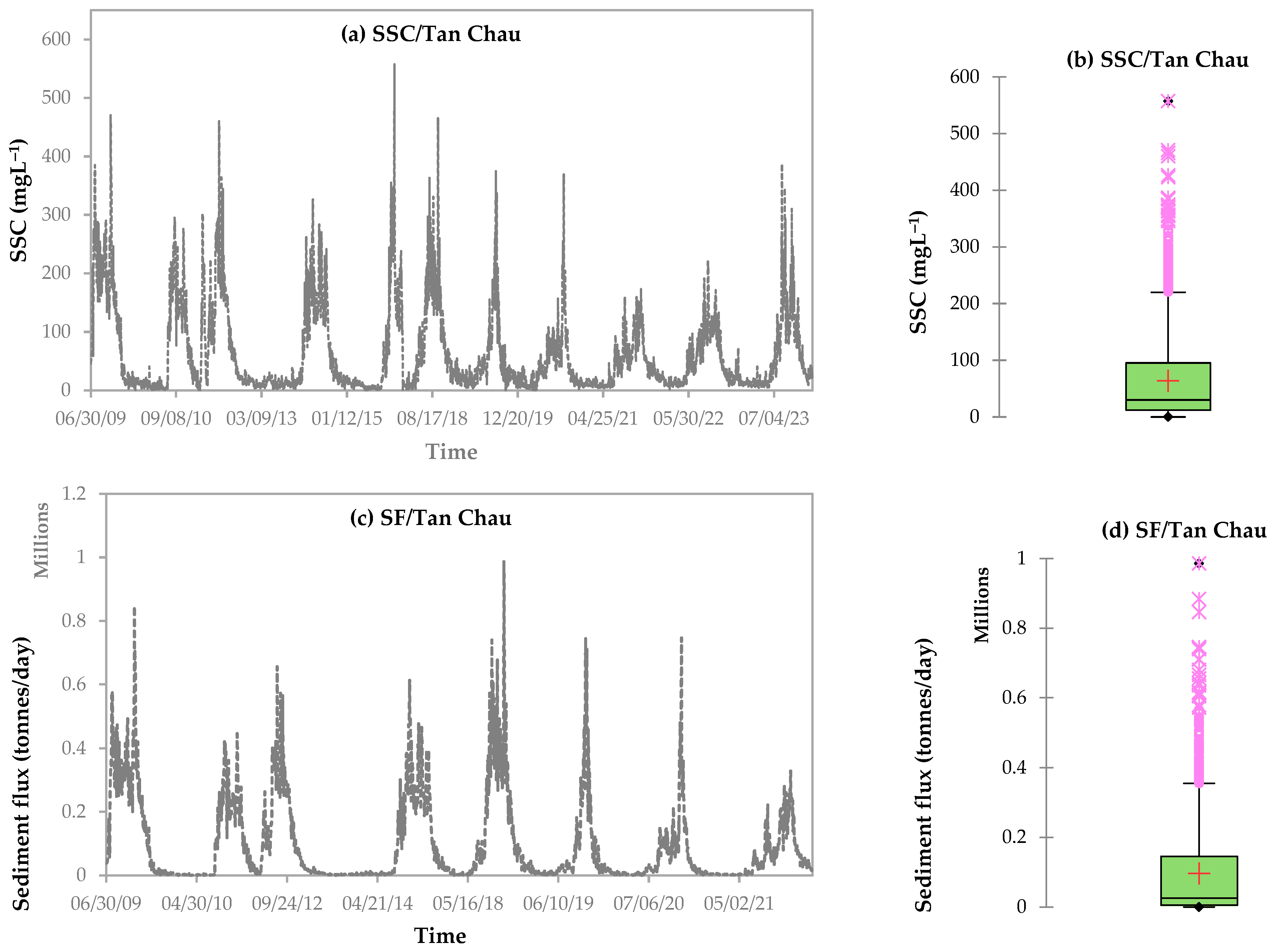
The distribution structure of SSC and SF at Tan Chau station exhibits typical positive skewness, reflecting an asymmetrical hydrological operating state. The median values remain low, with SSC around 30 mg/L and SF approximately 0.03 million tonnes/day, indicating that, for most of the monitoring period, concentrations and sediment load fluctuated only at the minimum baseline. This is reinforced by the internal variation range, in which 50% of the data are concentrated in the low-value range (SSC < 100 mg/L and SF < 0.15 million tonnes/day). These figures demonstrate the stable but sediment-poor state of the river throughout the dry season, which accounts for most of the year.
The dominance of outlier values plays a decisive role in the overall sediment dynamics of the system, with a high density of occurrence extending from the upper turret to the peak values (SSC around 560 mgL−1 and SF around 1.0 million tonnes/day). The continuous occurrence of outlier values, far from the average, clearly demonstrates the impact of hydrological pulses—short-term flood events that are the main factor in sediment mobilisation and transport.
Based on the time series data and empirical distribution plot in Figure 2, SSC and SF at Tan Chau are closely related and directly influenced by the hydrological regime of the Mekong River. Peak values are usually concentrated from July to November, coinciding with flood periods. During the flood season, SSC fluctuates from 200 to 400 mgL−1, driving SF up to 0.4–0.8 million tonnes/day. Notably, the outflow of SF has a significantly wider spread and higher concentration than SSC. This phenomenon confirms that water flow acts as a hydraulic multiplier, amplifying the concentration of suspended sediment into massive downstream loads.
The inter-year variation in flood peaks reflects the impact of extreme meteorological phenomena. During major flood years such as 2009, 2011, and 2018, the Tan Chau station recorded peak SF exceeding 0.8 million tonnes/day. Conversely, during El Niño phases like 2010 and 2015–2016, sediment transport capacity decreased by more than 50%, with peak SF limited to 0.4 million tonnes/day.
A noteworthy phenomenon is the phase difference between concentration and load. For example, although SSC reached a record high at the end of 2015 (>557.5 mgL−1), it did not produce a comparable SF peak in 2018. This confirms that SF is a function of both material concentration and the hydraulic impulse of the flow. Furthermore, the multi-peak structure observed in the SF diagram reflects the river system’s instantaneous response to short-term hydraulic impulses or unusual water regulation from upstream reservoir systems.
In the long term, empirical data from 2018 to 2022 show a clear downward trend in SSC peaks, notably in 2021, when the peak value remained below 200 mgL−1. Although there was a local recovery at the end of 2023 (approaching 400 mgL−1), sediment transport phases are generally showing a narrowing time breadth. This decline is entirely consistent with scientific evidence of sediment trapping at upstream hydropower dams. These empirical signals are vital indicators that must be continuously monitored to assess the future stability of the Mekong Delta’s geological and ecological systems.
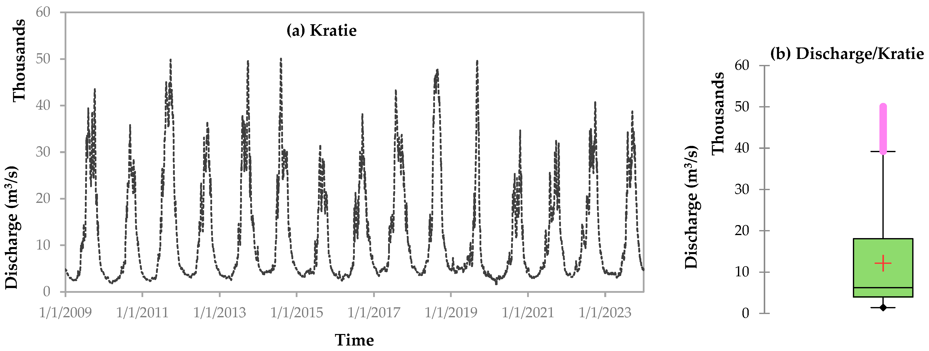
Figure 3a shows a pronounced seasonal cycle in Mekong River discharge at Kratie. Annual flood peaks typically occur between August and October, with discharges reaching approximately 40,000–50,000 m3/s, followed by a prolonged dry season during which discharge commonly falls below 10,000 m3/s. The corresponding box plot indicates a relatively low median discharge (7000–8000 m3/s), implying that for much of the year the river remains in lower-flow conditions, while the upper tail extending to ~50,000 m3/s reflects the magnitude of the monsoon flood pulse.
Across the key variables, discharge at Kratie and SSC and SF at Tan Chau, distributions are strongly right-skewed with long upper tails, consistent with the episodic dominance of high-flow events in driving sediment transport. Flood peaks at Kratie coincide with the largest downstream increases in SSC and SF at Tan Chau. Notably, while discharge at Kratie typically varies by a factor of 5–7 between dry-season conditions and flood peaks, SF at Tan Chau exhibits substantially greater variability, increasing by roughly an order of magnitude or more from typical values (<50,000 tonnes/day) to peak events approaching 1,000,000 tonnes/day. This amplification highlights the nonlinear nature of sediment transport relative to discharge.
Outliers in discharge at Kratie recur regularly and align closely with seasonal forcing. In contrast, high-end outliers in SSC and SF at Tan Chau are more frequent and more dispersed, indicating greater stochasticity in sediment responses. This suggests that predictive modelling of SSC and SF is more challenging than discharge alone, as sediment dynamics depend not only on hydrological forcing but also on sediment availability, antecedent conditions, and channel/floodplain processes that may vary interannually.
Numerous studies indicate that the highest rate of alluvial deposition in the Mekong Delta is concentrated in the river mouths and nearshore continental shelf, exceeding 10 cm/year. However, this figure gradually decreases with distance from the shore: in areas 20–50 km from the river mouth, the deposition rate is only 1–3 cm/year, and further decreases to a minimum of about 0.4 cm/year in the more distant continental shelf [53]. On average over the long term, the deposition rate across the region ranges from a few millimetres to tens of centimetres per year. However, since the 1990s, the deposition rate in the Mekong Delta has seriously declined due to the impact of upstream hydropower dam construction, sand mining, and land reclamation [54,55]. This situation has led to an imbalance between deposition and erosion. It is projected that by 2050–2060, the deposition rate in floodplains could decrease by an average of 40%. In the most extreme scenarios, the rate of sedimentation risks decreasing by as much as 90%, directly threatening the sustainable development of the delta region [55].
Two modelling datasets were prepared to support algorithm development: (i) a Tan Chau SSC dataset for predicting SSC at Tan Chau (denoted SSC_TC in Table 1), and (ii) a Tan Chau sediment-flux dataset for predicting SF at Tan Chau (denoted SF_TC in Table 2). After removing days with missing values across the required predictors and responses, the SSC dataset comprised 3380 complete daily observations (2009–2023), while the sediment-flux dataset comprised 2343 complete daily observations (2009–2021).
As summarised in Table 1, SSC_TC ranges from 0.1 to 557.5 with a mean of 63.8 and standard deviation of 73.7, indicating substantial dispersion relative to the mean (CV = 1.2). For SF (Table 2), SF_TC ranges from 71 to 986,429 with a mean of 96,553 and standard deviation of 136,502 (CV = 1.4), consistent with a strongly right-skewed, event-dominated transport regime.
Both datasets use the same set of hydrometric predictors, including Q_Kratie, Hmean_TC, and the daily minimum, mean, and maximum discharge at Tan Chau (Qmin_TC, Qmean_TC, Qmax_TC), all of which display considerable variability (Table 1 and Table 2). These negative values indicate periods of tidal backwater or reversal flow where the tidal energy overcomes the river discharge, causing water to flow upstream.
Pearson correlation coefficients were computed to quantify pairwise linear associations between the response variables and candidate predictors (Table 3 and Table 4). SSC_TC shows strong positive correlations with all hydrometric predictors, with the highest correlation observed for Q_Kratie (r = 0.793; Table 3). A similar pattern is evident for SF (SF_TC), where Q_Kratie again exhibits the strongest association with the response (r = 0.837; Table 4). These results indicate that upstream discharge at Kratie is a dominant correlate of downstream suspended-sediment dynamics at Tan Chau during the study period. In addition, substantial intercorrelation is evident among the Tan Chau discharge statistics (Qmin_TC, Qmean_TC, and Qmax_TC), reflecting a high degree of collinearity among these closely related flow descriptors. This multicollinearity is expected given that the three metrics are derived from the same daily discharge series and may therefore convey overlapping information.

3.2. Model Training and Hyperparameter Optimisation

The hyperparameter optimisation was performed separately for SSC and SF to ensure a fair comparison between models. The final optimised hyperparameters for all models are listed in Table 5.
For the RF model, hyperparameters were tuned for (i) the number of predictors randomly sampled at each split (mtry) and (ii) the minimum terminal node size (min_n). As summarised in Table 5, the optimal settings for SSC were mtry = 3 and min_n = 3, whereas for SF the optimal configuration was mtry = 5 and min_n = 3.
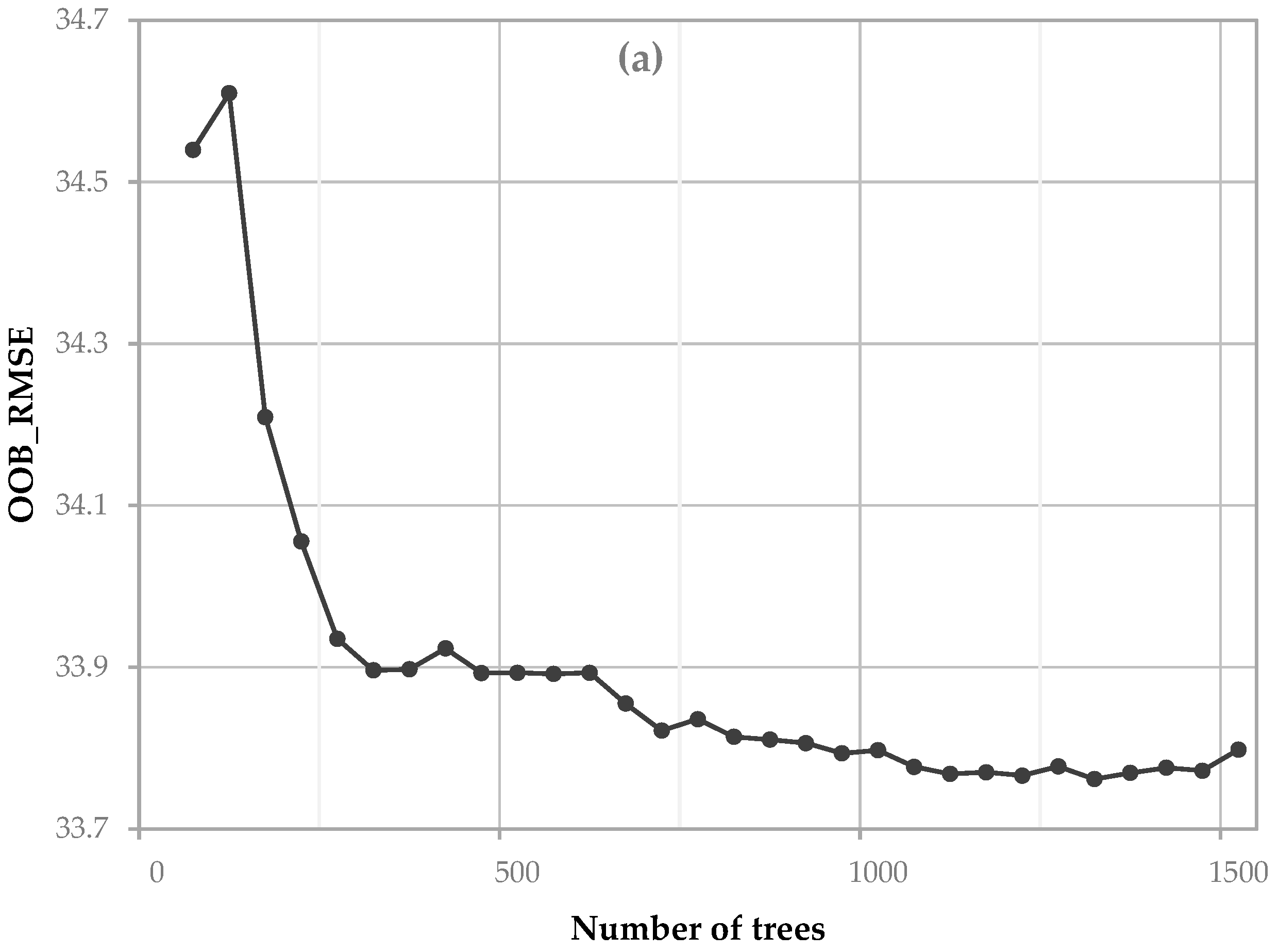
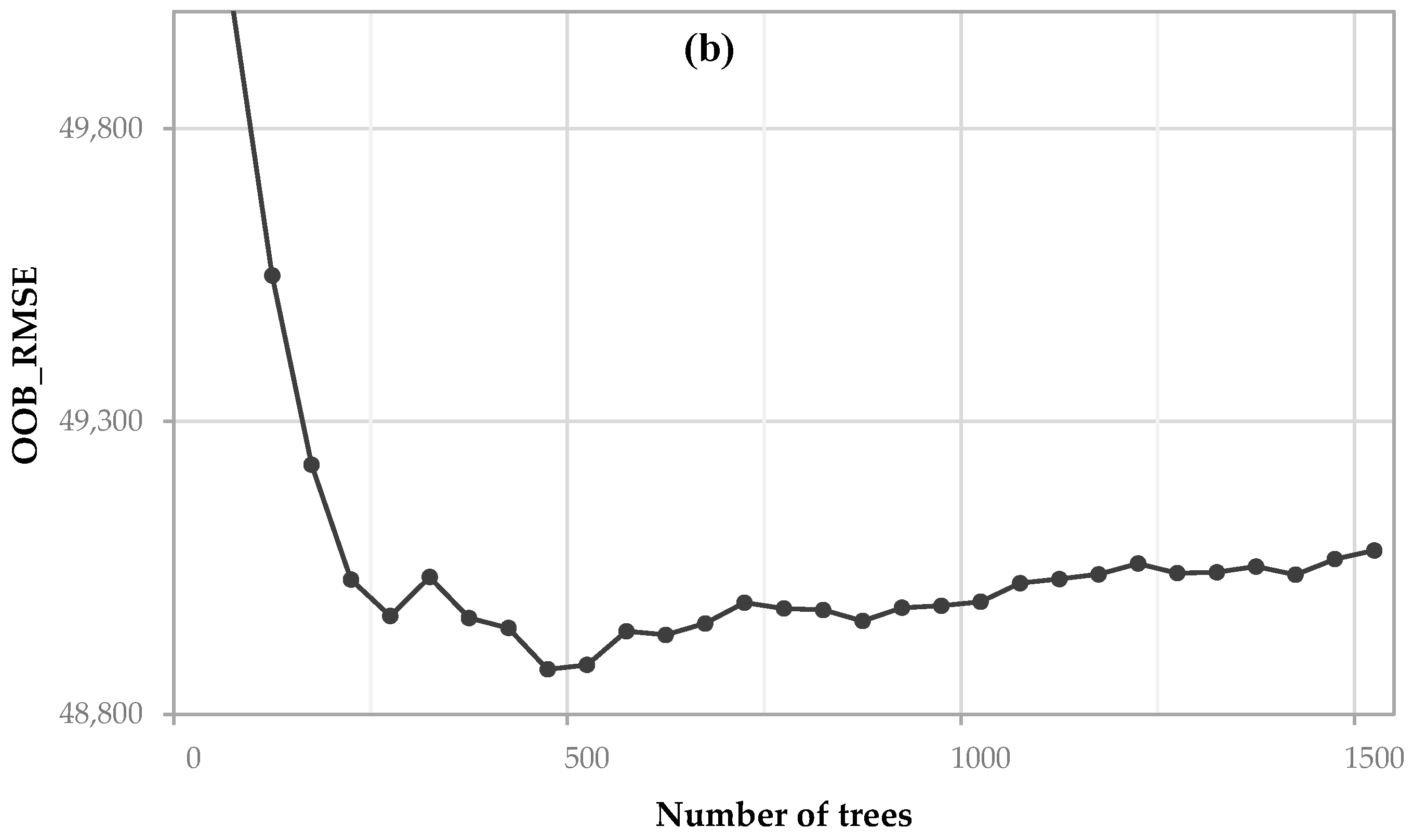
Figure 4 presents the out-of-bag (OOB) RMSE trajectories as the number of trees increases. In both cases, OOB error decreases rapidly during early model growth and then approaches an asymptote as additional trees contribute progressively smaller performance gains. For SC, the lowest OOB RMSE is achieved at approximately 1400 trees (Figure 4a), after which performance stabilises. For SF, the OOB RMSE reaches a local minimum around 450–500 trees (Figure 4b) before increasing slightly thereafter, suggesting diminishing returns and potential stochastic variability in the OOB estimate at higher tree counts.
For the XGBoost model, the hyperparameters including the learning rate (η), the minimum child weight ( w m i n ), and the maximum tree depth ( d m a x ) were systematically tuned to optimise performance. As reported in Table 5, the optimal configuration for the SSC model was η = 0.03, w m i n = 1 , and d m a x = 6 . Similarly, for the SF model, the optimal learning rate was slightly higher (η = 0.05), while the minimum child weight and maximum tree depth remained unchanged.
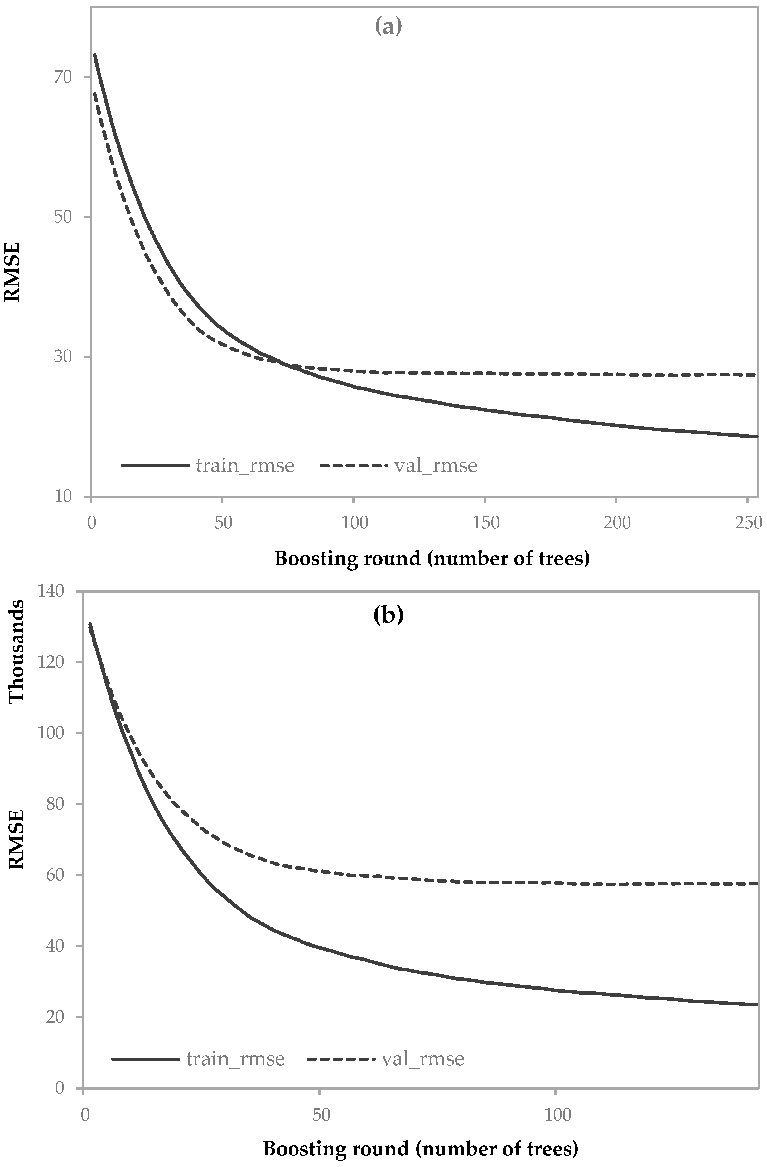
The training curve (Figure 5) illustrates the evolution of RMSE for the XGBoost model as a function of the two variables, SSC and SF. Overall, both models demonstrate rapid learning with high convergence rates in the early stages of training. For the SSC variable (Figure 5a), the RMSE on both the training and validation sets decreased sharply in the first 50 iterations. After approximately 100 iterations, the validation error stabilised at approximately 27.0, while the training error continued to decrease slightly, reaching 18.0 at the 250th iteration. The narrow gap between the two error curves indicates that the SSC model effectively controls overfitting and has the ability to generalise data stably. Conversely, the SF model (Figure 5b) shows a significantly higher absolute error margin due to the large variability of the sediment flow value. The validation error of the SF model reached saturation earlier, around the 75th iteration, and remained stable at approximately 58.0 (thousands). However, the training error curve dropped significantly below 25.0 by the end of the process, creating a wider gap than the SSC model. In both cases, validation error decreases rapidly during the early boosting iterations and then stabilises, indicating convergence. The absence of further improvement after convergence suggests that additional boosting iterations yield negligible generalisation gains under the selected hyperparameters and that model complexity is effectively controlled for the present data and feature set.
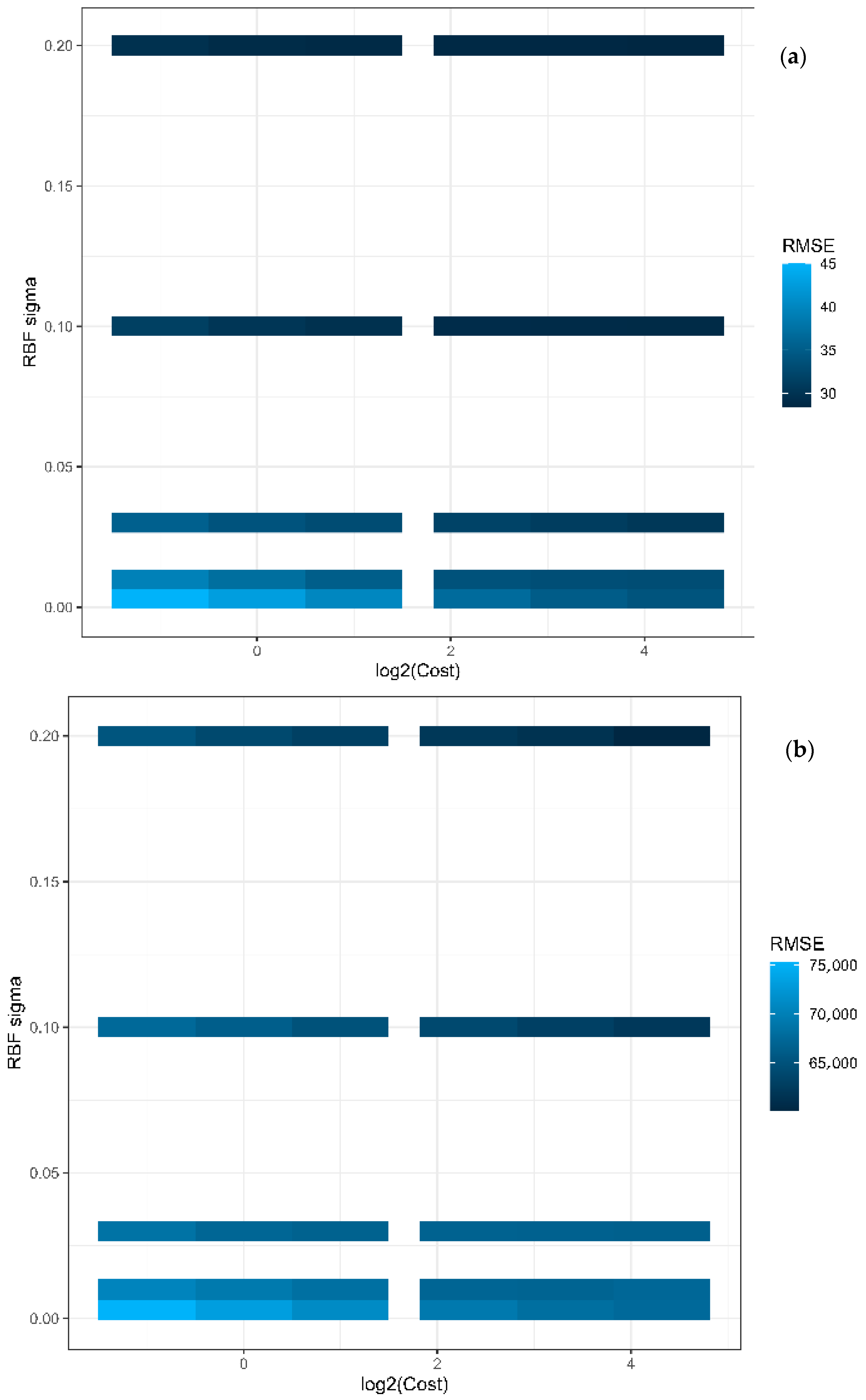
For the SVM model (support vector regression with a radial basis function kernel), hyperparameter tuning was conducted for the regularisation parameter (cost), the kernel width (rbf_sigma), and the ε-insensitive loss parameter (ε, hereafter “margin”) (Figure 6). As shown in Table 5, the optimal configuration was identical for both (SSC and SF: cost = 20, rbf_sigma = 0.2, and ε = 0.1.

3.3. Model Performance on Testing Data

Model performance on the held-out testing dataset is summarised in Table 6. Across all three algorithms, the relatively high R2 and NSE values indicate good agreement between predictions and observations in both variability and overall magnitude for the testing subset. Performance is consistently higher for SF than for SSC across all models. Specifically, SF prediction achieves R2 = 0.841–0.867 and NSE = 0.837–0.866, compared with SC prediction, which achieves R2 = 0.769–0.783 and NSE = 0.761–0.782.
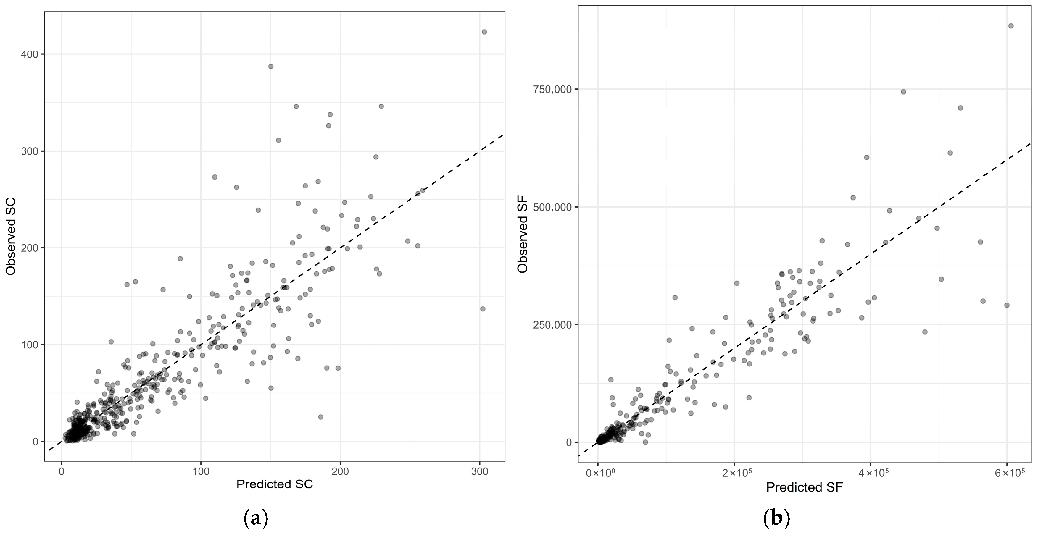
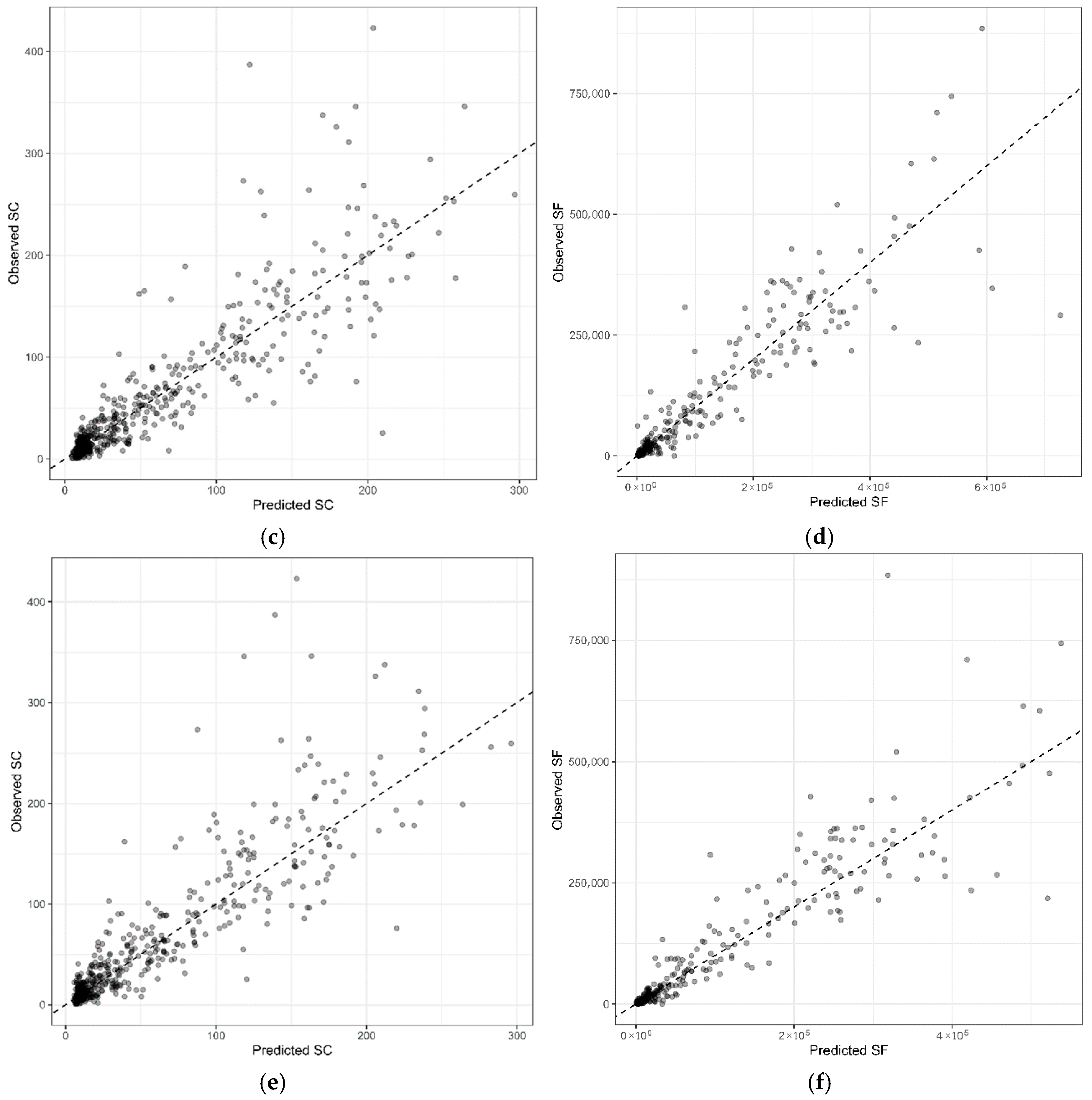
Figure 7 presents scatter plots of observed versus predicted SSC and SF for the testing dataset. For SC, the RF model achieves the best overall performance, with the lowest RMSE (33.643 mgL−1) and the highest R2 (0.783) and NSE (0.782). XGBoost performs comparably, with an RMSE of 34.266 mgL−1 and slightly lower R2/NSE (both 0.774). In contrast, SVM yields the highest RMSE (35.189 mgL−1) and the lowest R2 and NSE among the three models (Table 6). Visually, RF aligns most closely with the 1:1 line across the mid-range of concentrations (Figure 7a), while XGBoost shows slightly greater dispersion (Figure 7c) and SVM exhibits the widest spread across the concentration range (Figure 7e).
For SF, all models perform better than for SSC at Tan Chau station (Table 6). RF again provides the strongest results, with an RMSE of 51,433 tonnes/day and the highest R2 (0.867) and NSE (0.866). XGBoost ranks second (RMSE = 55,236 tonnes/day; R2 = 0.847; NSE = 0.846), followed by SVM (RMSE = 56,831 tonnes/day; R2 = 0.841; NSE = 0.837). The observed–predicted plots indicate that RF exhibits the closest correspondence to the 1:1 line (Figure 7b), with XGBoost showing broadly similar linearity but slightly greater scatter (Figure 7d). SVM displays the greatest dispersion (Figure 7f). Across all models, dispersion increases at higher flux values, indicating that extreme SF events remain the most difficult to reproduce accurately.

3.4. Variable Importance and Predictor Influence

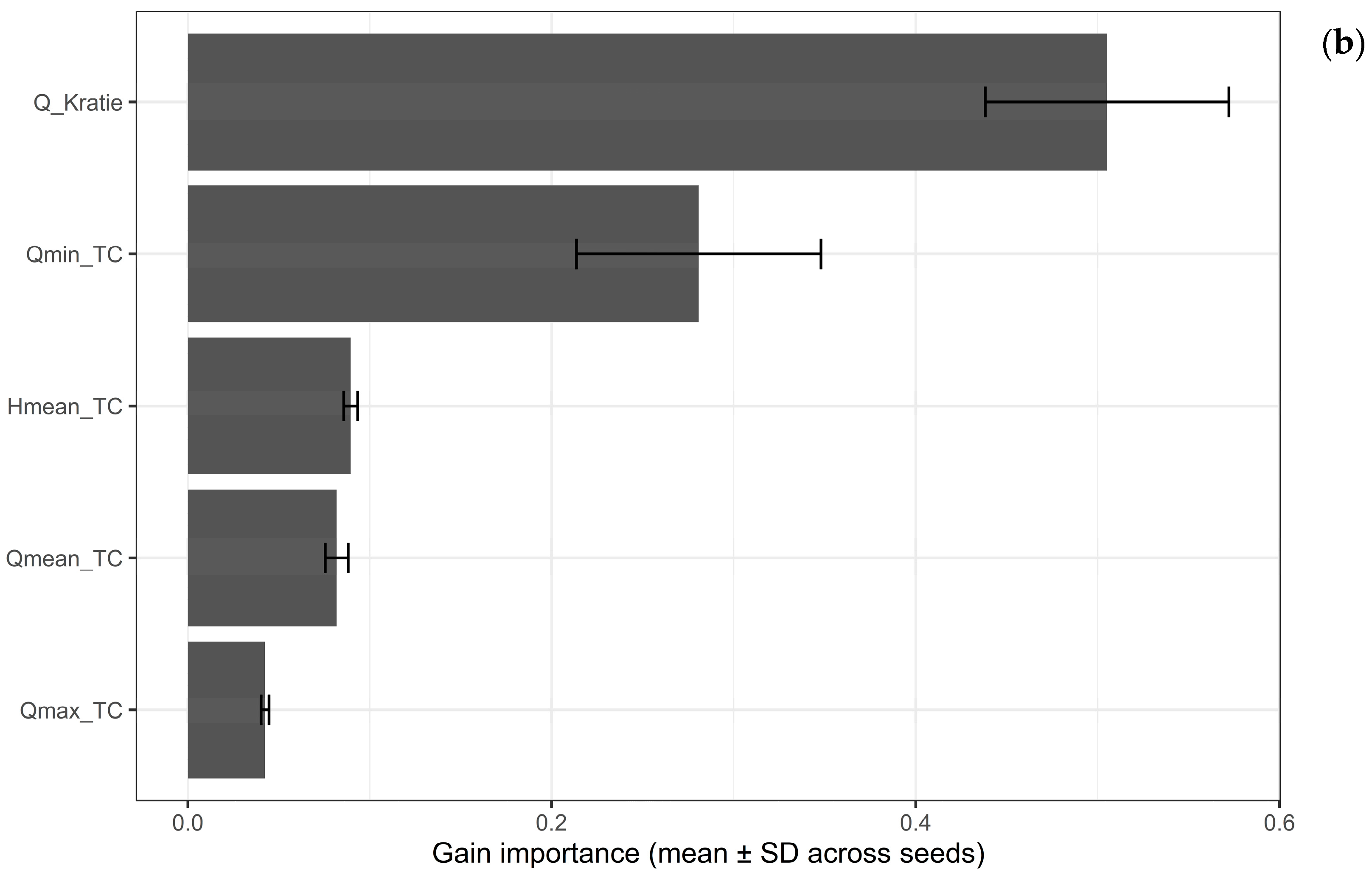
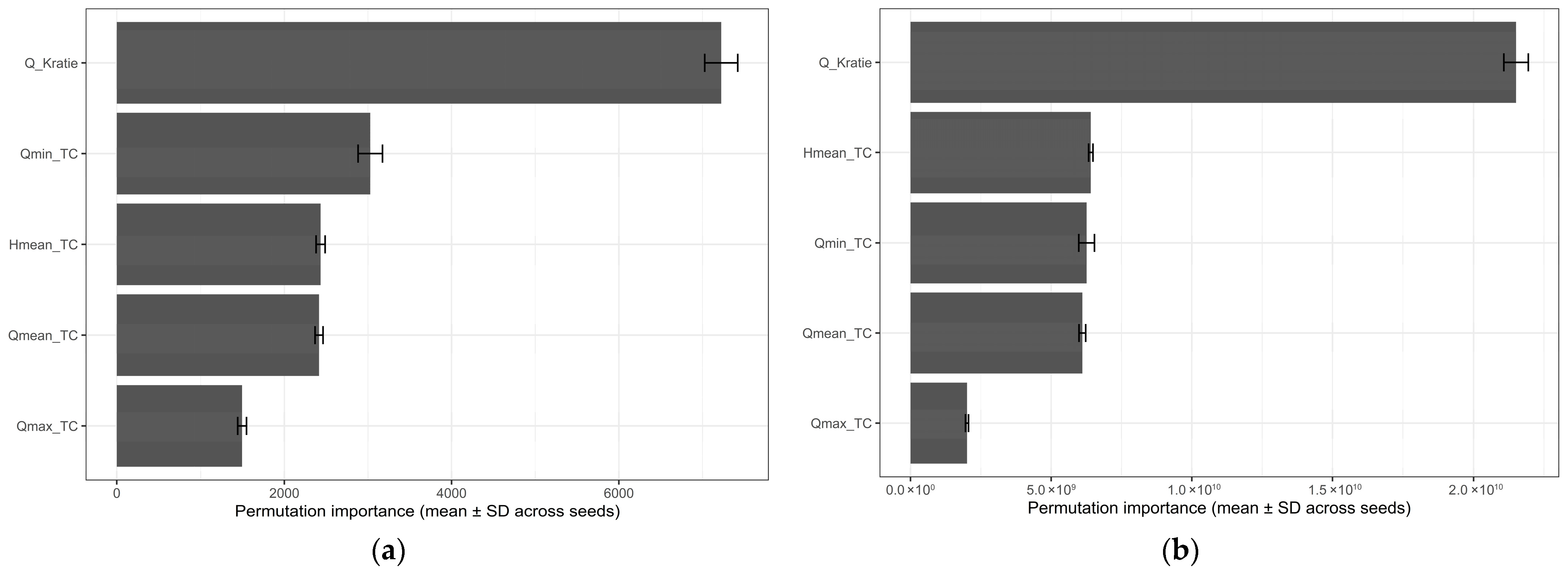
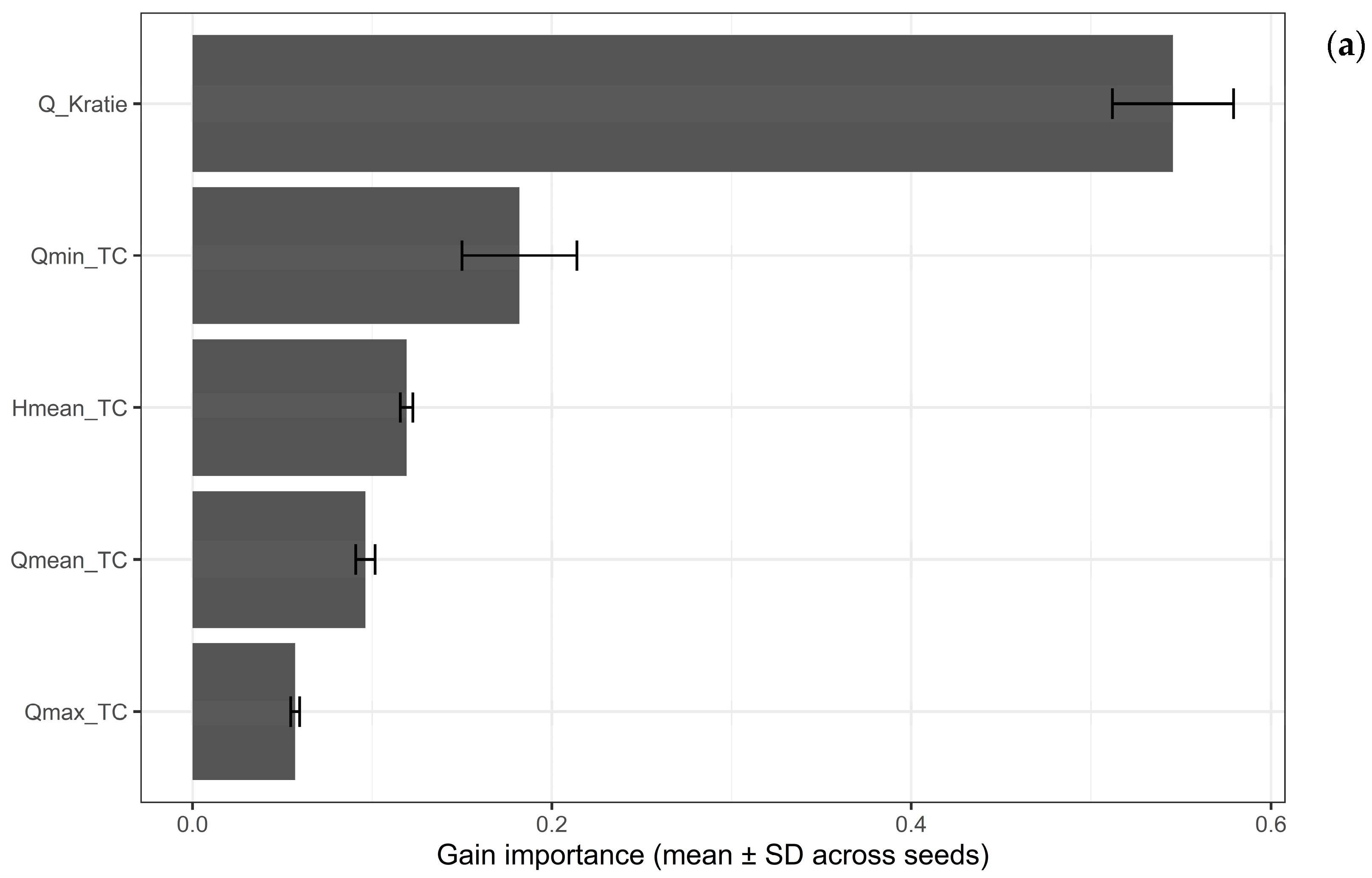
Variable-importance diagnostics were derived for the RF and XGBoost models to examine the relative contribution of each predictor to the prediction of SSC and SF. The resulting rankings are shown in Figure 8 (RF) and Figure 9 (XGBoost).
For SSC prediction, discharge-related predictors dominate in both models. In the RF model (Figure 8a), Q_Kratie and Qmean_TC exhibit the highest importance, followed by Qmin_TC and Qmax_TC, while Hmean_TC contributes comparatively less. In the XGBoost model (Figure 9a), gain is more evenly distributed across predictors, but the overall pattern is consistent with RF: Q_Kratie and Qmean_TC remain dominant, and Hmean_TC shows a more substantive contribution than in the RF ranking. Overall, SSC prediction draws on information from multiple hydrometric indicators (discharge and water level) rather than being controlled by a single predictor.
For SF prediction, predictor importance becomes more concentrated. In the RF model (Figure 8b), Q_Kratie is the most influential variable, with a clearer separation between Q_Kratie and the remaining predictors; Qmean_TC remains the next most important. The relative importance of Qmin_TC and Qmax_TC increases modestly compared with SSC prediction. In the XGBoost model (Figure 9b), gain is concentrated primarily on Q_Kratie and Qmean_TC, with the remaining predictors contributing less than in the SSC case.
Across both modelling frameworks, upstream discharge at Kratie (Q_Kratie) is consistently the highest-ranked predictor for both SSC and SF. Its dominance is more pronounced for SF than for SSC (Figure 8 and Figure 9), consistent with SF being directly conditioned by discharge and concentration dynamics. While RF produces a relatively stable and hierarchical importance ranking, XGBoost distributes importance more flexibly across predictors, reflecting differences in how the two algorithms partition and weight predictor contributions.
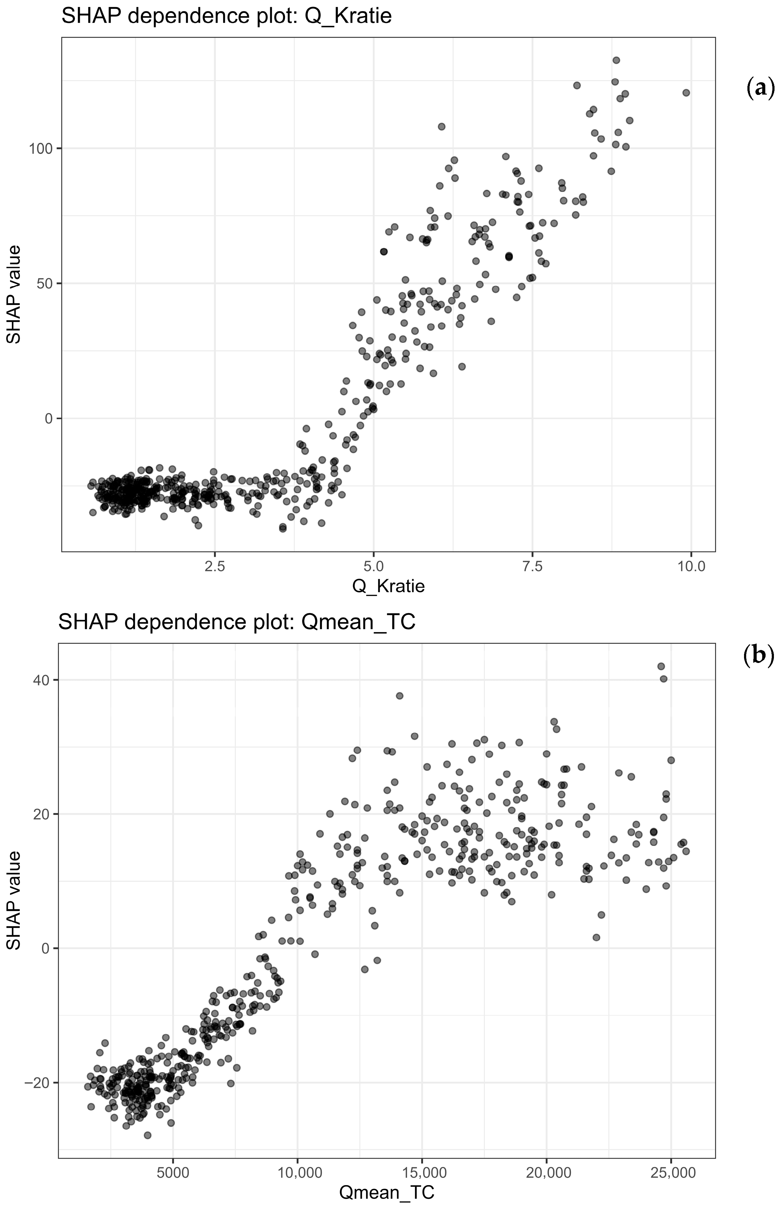
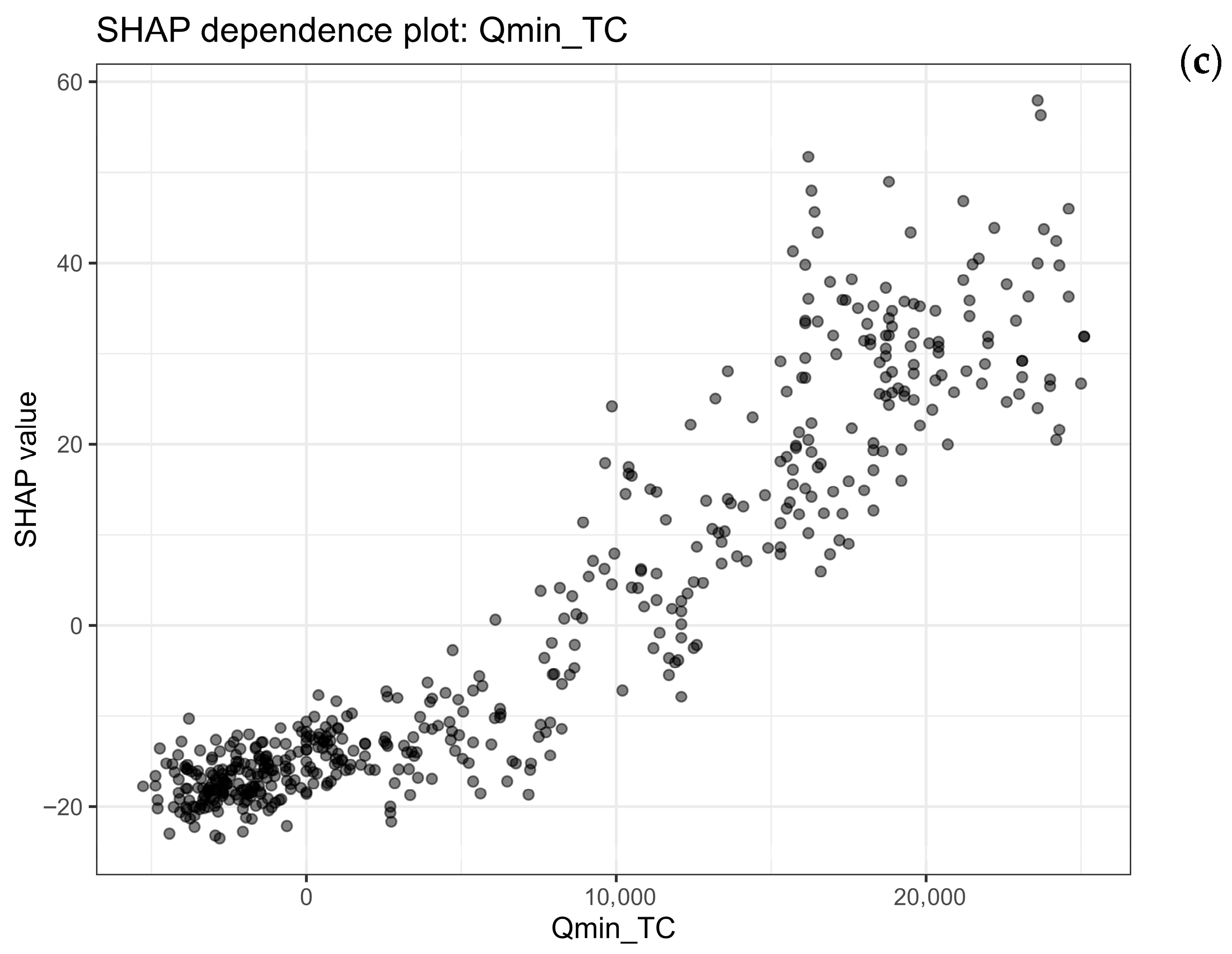
To clarify the model’s operating mechanism and its responsiveness to extreme hydrological scenarios, the study conducted a SHAP dependency analysis (Figure 10) to identify physical thresholds and multivariate interactions under high flow conditions.
The SHAP dependence of the Q_Kratie plot demonstrates the most pronounced non-linear impact on the forecasting model. Specifically (Figure 10a), the results show a critical physical threshold between 4000 and 5000 m3/s; at low flow levels below this threshold, the SHAP value remains stable at negative or near-zero levels, indicating a limited contribution of flow to sediment transport. However, when the flow rate exceeds 5000 m3/s, the SHAP value increases sharply with a steep slope. This phenomenon demonstrates that when flood flow reaches a certain energy level, the sediment transport capacity of the system is strongly activated, confirming the role of Q_Kratie as a key physical factor regulating sediment dynamics in extreme situations in the study area.
The SHAP of the Qmean_TC plot shows a gradual upward trend but with clear signs of saturation. Between flow rates of 5000 and 15,000 m3/s (Figure 10b), the contribution of this variable to the model increases rapidly, reflecting a positive correlation between local flow scale and sediment load. However, when flow rates exceed 15,000 m3/s, the graph tends to flatten, indicating that further increases in average flow at the measurement point no longer have a sudden impact on the forecast results. This characteristic suggests that Qmean_TC only partially reflects the system dynamics; when flood intensity reaches its peak, hydrological signals from upstream (Q_Kratie) become the primary determinant of the significant variations in sediment concentration and load.
The SHAP dependency plot of the Qmin_TC variable shows a continuous, non-linear positive correlation with the model’s forecasting results. Unlike the threshold characteristic of the Q_Kratie variable or the saturation trend after the 15,000 threshold of the Qmean_TC variable, the contribution of Qmin_TC maintains a stable growth momentum across the entire observed range (Figure 10c). This characteristic confirms the dominant and consistent role of minimum flow in determining the output forecast value. However, in the high value segment above 15,000, this variable shows significantly greater vertical dispersion compared to the other variables. This phenomenon reflects the presence of complex interaction effects between Qmin_TC and other input characteristics. This indicates that in high-flow scenarios, the impact of Qmin_TC is no longer linearly independent but becomes a reciprocal component, closely dependent on the overall coordination state of the hydrological system in the model.

4. Discussion

4.1. Comparative Performance of ML Models for Sediment Prediction

This study indicates that data-driven models effectively capture daily variations in SSC and SF at Tan Chau. By utilising discharge data from Kratie and local hydrometric inputs (discharge and water level), these models achieve high predictive accuracy with minimal complexity. Across all models, performance is consistently higher for SF (R2 = 0.84–0.87; NSE 0.84–0.87) than for SSC (R2 = 0.77–0.78; NSE = 0.76–0.78). Field measurements indicate that while streamflow follows predictable seasonal patterns, sediment deposition on floodplains varies drastically from 2.2 to 60 kg/m2/yr [7,8,56]. This variance is linked to localised factors such as the extensive dyke systems in the VMD, which reduce sediment retention to a mere 1–6% compared to 19–23% in natural floodplains [57]. These within-channel and floodplain exchange processes, alongside localised erosion reaching up to 500 m/yr in certain hotspots, confirm that SSC at Tan Chau is heavily influenced by supply-limited dynamics and morphodynamic factors rather than a simple transport-capacity signal [58].
Among the evaluated algorithms, RF provides the best overall predictive skill for both SSC and flux, followed closely by XGBoost, while SVM performs the worst. The RF advantage is consistent with its ensemble structure and its capacity to learn nonlinear relationships in noisy environmental datasets. Specifically, RF can capture complex and threshold-driven dynamics between discharge and SSC as well as multi predictor interactions such as seasonal or tidal modulation of sediment transport without requiring explicit functional forms [48,59].
XGBoost exhibits efficient complexity management and fast convergence, thanks to the optimisation of core hyperparameters such as learning rate ( η ), gamma ( γ ), and subsampling [51]. In other settings, gradient boosting can outperform bootstrap aggregation techniques when subtle interactions and non-linearities dominate; here, the marginal gap between RF and XGBoost plausibly reflects the limited predictor set and the dominance of discharge controls that both algorithms capture well [3,60]. The weaker SVM performance may indicate that the mapping from hydrometric inputs to sediment outcomes is characterised by non-linear threshold behaviour—such as the critical discharge levels required to initiate sediment motion—and complex interaction structures between upstream and local variables. Tree-based ensembles (RF and XGBoost) are inherently better suited to represent these dynamics than a single kernel-based SVM. While SVM attempts to find a global optimal hyperplane, tree models effectively partition the feature space into discrete decision rules (e.g., if Discharge > Threshold), which more naturally capture the abrupt changes in sediment concentration during flash floods or seasonal transitions. Consequently, the tree ensembles can resolve the conditional dependencies between discharge and sediment availability that a single kernel function within the current feature space may fail to approximate [35,61,62].
From an application perspective, the achieved NSE/R2 values indicate performance that would generally be regarded as “good” for hydrological prediction tasks, particularly given the heavy-tailed nature of sediment data [33,63]. This heavy-tailed distribution implies that sediment transport is dominated by infrequent but high-magnitude events, as clearly reflected in the scatter plots in Figure 7. While the models capture the overall trend, there is a visible dispersion at high-flux values, where the points spread farther from the 1:1 line. This residual variance is consistent with event-dominated transport mechanisms, where a small number of extreme events contribute disproportionately to the total sediment load and remain difficult to predict using hydrometric predictors alone [7,27]. Consequently, the model performance in Figure 7 demonstrates a robust capture of baseflow and moderate transport, while highlighting the inherent stochasticity associated with peak sediment concentrations.

4.2. Hydrological Controls and the Meaning of Variable Importance

Variable importance results indicate that discharge controls dominate prediction performance, with upstream discharge at Kratie identified as the most influential predictor for both SSC and SF across both RF and XGBoost rankings. This finding is physically plausible and aligns with the Mekong system understanding, as Kratie acts as a key control point that integrates basin-scale hydrological forcing before flows propagate into the Cambodian floodplain and the Vietnamese delta distributary network [8]. Seasonal flood pulses, modulated by monsoon variability and upstream regulation, govern downstream transport capacity and the timing of sediment delivery. Historically, the Mekong River transported approximately 160 million tonnes of sediment annually, with over 90% of this total load delivered during the high-flow season (June to November) [7,27,64]. The strong correlation between Q_Kratie and both SSC and flux at Tan Chau (r ≈ 0.79 to 0.84) reinforces this role and is consistent with studies that derive or constrain sediment dynamics through discharge-based relationships in the Lower Mekong [65]. These dynamics are characterised by non-linear threshold behaviour and pronounced seasonality, where hydrological energy dictates both the timing and magnitude of sediment delivery.
At the same time, the models provide additional explanatory power by assigning significant predictive weight to local Tan Chau discharge statistics and Hmean_TC, particularly for SSC. SF prediction is more hydraulically driven, whereas SSC prediction is more process mixed: discharge sets the transport envelope, but SSC responds more strongly to sediment availability and local mixing processes [7,57]. While XGBoost typically distributes predictions more broadly across features than the more concentrated importance profiles of RF, both methods identify a consistent hierarchy of controls. The shared prominence of Q_Kratie and Q_meanTC suggests that these variables represent the primary physical drivers of the system. Specifically, Q_Kratie serves as the regional boundary condition that governs total water and sediment influx, while Q_mean_TC acts as a local hydraulic regulator that reflects the interaction between fluvial flow and downstream tidal constraints. This stability across different ML architectures reinforces the physical validity of the model’s selected features.
The dominant role of river discharge in controlling SSC and SF observed in the VMD is consistent with hydrological patterns documented in major deltaic systems globally. In the Mississippi River, historical data indicate that water discharge remains the primary driver of sediment transport capacity, even as total sediment loads have declined due to upstream engineering [66]. Similarly, in the Amazon basin, the largest river system in the world, river discharge accounts for over 90% of the variability in annual SF to the Atlantic Ocean [67,68]. In tide-influenced deltas like the Ganges Brahmaputra, extreme discharge events during the monsoon season are responsible for the vast majority of sediment delivery to the delta plain [69,70]. These global comparisons confirm that while localised factors such as tidal modulation or human interventions like sand mining can alter concentration levels, the fundamental energy for sediment transport is dictated by the upstream discharge regime. Ultimately, the ability of ML-based models to capture these dynamics provides a critical tool for managing sediment starvation and enhancing delta resilience in the face of non-stationary environmental changes.

4.3. Declining Sediment Peaks and Implications for Delta Risk and Management

The observed attenuation of SSC peaks after ~2017 (notably 2018–2022) provides an empirical signal consistent with the broader narrative of sediment decline in the Lower Mekong. Multiple lines of evidence indicate that reservoir trapping, altered hydrological seasonality, and sand extraction have reduced downstream sediment continuity and reshaped sediment pathways across the Mekong–Tonle Sap–delta continuum [21,22,23,24,44,45]. Recent work also documents downstream expressions of this sediment-starvation signal, including reduced sediment delivery to coastal waters and changes in plume dynamics [45], as well as long-term weakening of sediment–discharge relations under hydropower development [39]. While the present study does not attribute causality, the observed time-series behaviour at Tan Chau is consistent with these system-wide pressures.
Within this context of the Lower Mekong Basin, ML-based prediction is not an end in itself but a potential contribution to operational sediment governance. Reliable short-horizon prediction of SSC/flux can support: (i) early warning for high-turbidity events relevant to water intake and treatment in downstream areas; (ii) timing and targeting of navigation dredging and maintenance; (iii) situational awareness for bank-protection planning in erosion-prone reaches; and (iv) improved monitoring of sediment-starvation trajectories that inform sand-mining. The strong influence of upstream discharge also suggests a practical monitoring logic: maintaining high quality hydrometric and sediment observations at key control points such as Kratie and delta entry stations remains foundational for both modelling and management.

4.4. Limitations and Priorities for Future Work

Several limitations should be acknowledged. First, although random 70/15/15 splitting facilitates a controlled comparison across algorithms, daily hydrological series exhibit serial dependence; random splitting can therefore yield optimistic estimates of generalisation when training and test sets contain temporally adjacent observations [71,72]. This is particularly relevant in a system subject to non-stationarity arising from infrastructure expansion, changing sediment availability, and climate variability. Future work should therefore complement random splitting with time-aware evaluation (e.g., blocked or rolling-origin splits) to assess robustness under regime shifts and to better represent operational forecasting conditions [71,72].
Interpretability based on variable importance can be sensitive to predictor correlation and the specific importance metric used; this is especially relevant where multiple discharge descriptors are highly collinear [73,74]. Where decision support requires clearer attribution, future analyses could complement global importance with more diagnostic, local interpretability tools (e.g., SHAP values) to examine how predictors influence predictions across flow regimes and extremes [75].
The strongest prediction errors occur during extreme-flux events, indicating that current predictors may not fully capture event-scale sediment availability, bank-erosion pulses, tidal-phase effects, or rapid land-use change. These limitations motivate three feasible extensions: (i) incorporating tidal descriptors or harmonics in tide-influenced reaches; (ii) adding rainfall, antecedent wetness, or upstream reservoir-operation proxies where available; and (iii) integrating remote-sensing indicators of turbidity/sediment and floodplain inundation dynamics to provide spatial context beyond point stations [15,76]. To extend this study, we intend to incorporate additional factors, such as land-use changes and dam operating schedules, into the ML framework. Furthermore, we plan to test the model’s performance across different time scales, ranging from hourly alerts for high turbidity events to long-term decadal trends of sediment starvation in the VMD. A further limitation of this study is that model validation was conducted using withheld data from the same station rather than fully independent external observations. Although this approach is suitable for assessing internal predictive performance, it does not establish the models’ transferability across the wider VMD, where sediment dynamics exhibit strong spatio-temporal variability. Future research should therefore test model robustness using independent records from other stations, cross-station validation, and, where possible, field-based sediment measurements.
Finally, the modelling framework presented in this paper is intentionally focused and does not incorporate a full sensitivity analysis or a broader range of potential drivers beyond the selected hydrometric predictors. Variables such as rainfall, tidal characteristics, reservoir operation signals, land-use change, and channel morphological dynamics may also influence SSC and SF variability, but were beyond the scope of the current dataset and model design. Future research should extend the framework by incorporating these additional controls and by evaluating their relative influence more systematically.

5. Conclusions

This study demonstrates that RF and XGBoost models effectively capture the daily variability of both SSC and SF at Tan Chau, using a unified set of upstream and local hydrometric predictors. Across the held-out testing data, RF achieved the highest overall performance for both targets, with XGBoost performing comparably and SVM consistently ranking third. The models achieved higher predictive accuracy for SF compared to SSC. This occurs because SF is primarily driven by discharge, whereas SSC involves more complex variables such as sediment availability and exchange processes between the channel and the floodplain.
Variable-importance results indicate that discharge controls dominate prediction performance, with upstream discharge at Kratie emerging as the most influential predictor for both SSC and SF. This finding is physically plausible for the Mekong system and reinforces the role of basin-scale hydrological forcing propagating into the delta distributary network. Importantly, the dominant role of river discharge observed here aligns with global hydrological patterns documented in other major deltaic systems, such as the Mississippi, Amazon, and Ganges-Brahmaputra. In these diverse environments, despite varying degrees of human intervention or tidal influence, the upstream discharge regime remains the fundamental driver of sediment transport energy. At the same time, local Tan Chau discharge descriptors and water level provide additional explanatory power, highlighting the importance of combining upstream boundary conditions with delta-entry hydraulics when modelling sediment dynamics in a tide-influenced environment.
The observed record at Tan Chau shows an attenuation of wet-season SSC peaks during 2018–2022 compared with earlier years, with only partial recovery in 2023. While this study does not attribute causality, the pattern is consistent with broader concerns about reduced sediment continuity in the Lower Mekong, associated with upstream regulation and intensive in-channel extraction. From a risk management perspective, the findings underscore that the continued suppression of upstream sediment delivery exacerbates sediment starvation across the VMD. This deficit, characterised by the dramatic decline in annual sediment load from historical levels to approximately half, directly triggers widespread riverbed incision and chronic bank instability along the Mekong River (Tien River) and Bassac River (Hau River). Consequently, the ongoing loss of mineral sediment deposition weakens the delta’s natural capacity to maintain its elevation, posing a critical threat to delta resilience. These results emphasise the urgent need for integrated management strategies that account for both hydrological changes and sediment supply to safeguard this rapidly developing yet subsiding region.
Overall, the results suggest that ML-based SSC and SF prediction models can complement monitoring efforts and provide actionable evidence to support sediment-aware decision-making in the VMD. Future work should test time-aware validation strategies and incorporate additional predictors relevant to event-scale sediment availability such as tidal descriptors, antecedent rainfall, or remotely sensed turbidity. These additions are expected to strengthen robustness under non-stationary conditions and improve model performance during extreme transport events.

Author Contributions

Conceptualization, N.P.C., N.K.D. and P.K.; methodology, N.P.C., N.K.D., H.V.T.M., T.V.H., P.C.N. and P.K.; software, N.P.C. and P.C.N.; writing—original draft preparation, N.P.C., T.V.H., N.K.D. and P.K.; and writing—review and editing, H.V.T.M., N.K.D. and P.K. All authors have read and agreed to the published version of the manuscript.

Funding

This research received no external funding.

Data Availability Statement

The original contributions presented in this study are included in the article. Further inquiries can be directed to the corresponding author.

Conflicts of Interest

The authors declare no conflicts of interest.

References

  1. Asadi, H.; Dastorani, M.T.; Khosravi, K.; Sidle, R.C. Applying the C-Factor of the RUSLE Model to Improve the Prediction of Suspended Sediment Concentration Using Smart Data-Driven Models. Water 2022, 14, 3011. [Google Scholar] [CrossRef]
  2. Lund, J.W. Using Machine Learning to Improve Predictions and Provide Insight into Fluvial Sediment Transport. Hydrol. Process. 2022, 36, e14648. [Google Scholar] [CrossRef]
  3. Miao, J.; Zhang, X.; Zhang, G.; Wei, T.; Zhao, Y.; Ma, W.; Chen, Y.; Li, Y.; Wang, Y. Applications and Interpretations of Different Machine Learning Models in Runoff and Sediment Discharge Simulations. Catena 2024, 238, 107848. [Google Scholar] [CrossRef]
  4. Minh, H.V.T.; Nam, N.D.G.; Ngan, N.V.C.; Van Thinh, L.; Nam, T.S.; Van Cong, N.; Nhat, G.M.; Lien, B.T.B.; Kumar, P.; Downes, N.K. Is Vietnam’s Mekong Delta Facing Wet Season Droughts? Earth Syst. Environ. 2024, 8, 963–995. [Google Scholar] [CrossRef]
  5. Minh, H.V.T.; Nam, N.D.G.; Nam, T.S.; Van Cong, N.; Kumar, P.; Downes, N.K. Transition of Flooding Patterns and Environmental Flow in the Mekong Delta, Vietnam over the Last 2 Decades. Nat. Hazards 2025, 121, 12665–12694. [Google Scholar] [CrossRef]
  6. Nourani, V.; Gökçekuş, H.; Gelete, G. Estimation of Suspended Sediment Load Using Artificial Intelligence-Based Ensemble Model. Complexity 2021, 2021, 6633760. [Google Scholar] [CrossRef]
  7. Manh, N.V.; Dung, N.V.; Hung, N.N.; Merz, B.; Apel, H. Large-Scale Suspended Sediment Transport and Sediment Deposition in the Mekong Delta. Hydrol. Earth Syst. Sci. 2014, 18, 3033–3053. [Google Scholar] [CrossRef]
  8. Thi Ha, D.; Ouillon, S.; Van Vinh, G. Water and Suspended Sediment Budgets in the Lower Mekong from High-Frequency Measurements (2009–2016). Water 2018, 10, 846. [Google Scholar] [CrossRef]
  9. Erban, L.E.; Gorelick, S.M.; Zebker, H.A. Groundwater Extraction, Land Subsidence, and Sea-Level Rise in the Mekong Delta, Vietnam. Environ. Res. Lett. 2014, 9, 084010. [Google Scholar] [CrossRef]
  10. Eslami, S.; Hoekstra, P.; Nguyen Trung, N.; Ahmed Kantoush, S.; Van Binh, D.; Duc Dung, D.; Tran Quang, T.; van der Vegt, M. Tidal Amplification and Salt Intrusion in the Mekong Delta Driven by Anthropogenic Sediment Starvation. Sci. Rep. 2019, 9, 18746. [Google Scholar] [CrossRef]
  11. Minderhoud, P.S.; Erkens, G.; Pham, V.; Bui, V.T.; Erban, L.; Kooi, H.; Stouthamer, E. Impacts of 25 Years of Groundwater Extraction on Subsidence in the Mekong Delta, Vietnam. Environ. Res. Lett. 2017, 12, 064006. [Google Scholar] [CrossRef]
  12. Minh, H.V.T.; Ngoc, D.T.H.; Lien, B.T.B.; Diep, N.T.H.; Nguyen, P.C.; Thanh, N.T.; Lavane, K.; Downes, N.K.; Kumar, P. Freshwater–Salinity Regime Shifts in the Vietnamese Mekong Delta: Multi-Decadal Trends and Emerging Risks (2000–2024). Environ. Geochem. Health 2026, 48, 139. [Google Scholar] [CrossRef] [PubMed]
  13. Tri, V.P.D.; Yarina, L.; Nguyen, H.Q.; Downes, N.K. Progress toward Resilient and Sustainable Water Management in the Vietnamese Mekong Delta. Wiley Interdiscip. Rev. Water 2023, 10, e1670. [Google Scholar] [CrossRef]
  14. Apel, H.; Hung, N.N.; Long, T.T.; Tri, V.K. Flood Hydraulics and Suspended Sediment Transport in the Plain of Reeds, Mekong Delta; Springer: Dordrecht, The Netherlands, 2012; pp. 221–232. [Google Scholar]
  15. Wackerman, C.; Hayden, A.; Jonik, J. Deriving Spatial and Temporal Context for Point Measurements of Suspended-Sediment Concentration Using Remote-Sensing Imagery in the Mekong Delta. Cont. Shelf Res. 2017, 147, 231–245. [Google Scholar] [CrossRef]
  16. Schmitt, R.; Giuliani, M.; Bizzi, S.; Kondolf, G.M.; Daily, G.C.; Castelletti, A. Strategic Basin and Delta Planning Increases the Resilience of the Mekong Delta under Future Uncertainty. Proc. Natl. Acad. Sci. USA 2021, 118, 2026127118. [Google Scholar] [CrossRef]
  17. Duy, D.V.; Ty, T.V.; Phat, L.T.; Minh, H.V.; Thanh, N.T.; Downes, N.K. Assessing River Corridor Stability and Erosion Dynamics in the Mekong Delta: Implications for Sustainable Management. Earth 2025, 6, 34. [Google Scholar] [CrossRef]
  18. Minh, H.; Kumar, P.; Downes, N.; Toan, N.; Meraj, G.; Nguyen, P.; Le, K.; Ty, T.; Lavane, K.; Avtar, R. Multi-Scale Characteristics of Drought Propagation from Meteorological to Hydrological Phases: Variability and Impact in the Upper Mekong Delta, Vietnam. Nat. Hazards 2024, 121, 2747–2779. [Google Scholar] [CrossRef]
  19. Ty, T.V.; Duy, D.V.; Phat, L.T.; Minh, H.V.T.; Thanh, N.T.; Uyen, N.T.N.; Downes, N.K. Coastal Erosion Dynamics and Protective Measures in the Vietnamese Mekong Delta. J. Mar. Sci. Eng. 2024, 12, 1094. [Google Scholar] [CrossRef]
  20. Van Binh, D.; Kantoush, S.A.; Ata, R.; Tassi, P.; Nguyen, T.V.; Lepesqueur, J.; Abderrezzak, K.E.K.; Bourban, S.E.; Nguyen, Q.H.; Phuong, D.N.L. Hydrodynamics, Sediment Transport, and Morphodynamics in the Vietnamese Mekong Delta: Field Study and Numerical Modelling. Geomorphology 2022, 413, 108368. [Google Scholar] [CrossRef]
  21. Kondolf, G.M.; Annandale, G.W.; Rubin, Z. Sediment Starvation from Dams in the Lower Mekong River Basin: Magnitude of the Effect and Potential Mitigation Opportunities. In Proceedings of the 36th IAHR World Congress, The Hague, The Netherlands, 28 June–3 July 2015. [Google Scholar]
  22. Kondolf, G.M.; Rubin, Z.K.; Minear, J. Dams on the Mekong: Cumulative Sediment Starvation. Water Resour. Res. 2014, 50, 5158–5169. [Google Scholar] [CrossRef]
  23. Bussi, G.; Darby, S.E.; Whitehead, P.G.; Jin, L.; Dadson, S.J.; Voepel, H.E.; Vasilopoulos, G.; Hackney, C.R.; Hutton, C.; Berchoux, T.; et al. Impact of Dams and Climate Change on Suspended Sediment Flux to the Mekong Delta. Sci. Total Environ. 2021, 755, 142468. [Google Scholar] [CrossRef]
  24. Kummu, M.; Lu, X.; Wang, J.-J.; Varis, O. Basin-Wide Sediment Trapping Efficiency of Emerging Reservoirs along the Mekong. Geomorphology 2010, 119, 181–197. [Google Scholar] [CrossRef]
  25. Gruel, C.-R.; Park, E.; Switzer, A.D.; Kumar, S.; Ho, H.L.; Kantoush, S.; Van Binh, D.; Feng, L. New Systematically Measured Sand Mining Budget for the Mekong Delta Reveals Rising Trends and Significant Volume Underestimations. Int. J. Appl. Earth Obs. Geoinf. 2022, 108, 102736. [Google Scholar] [CrossRef]
  26. Park, E. Sand Mining in the Mekong Delta: Extent and Compounded Impacts. Sci. Total Environ. 2024, 924, 171620. [Google Scholar] [CrossRef] [PubMed]
  27. Darby, S.E.; Hackney, C.; Leyland, J.; Kummu, M.; Lauri, H.; Parsons, D.R.; Best, J.L.; Nicholas, A.; Aalto, R. Fluvial Sediment Supply to a Mega-Delta Reduced by Shifting Tropical-Cyclone Activity. Nature 2016, 539, 276–279. [Google Scholar] [CrossRef]
  28. Idrees, M.B.; Jehanzaib, M.; Kim, D.; Kim, T.-W. Comprehensive Evaluation of Machine Learning Models for Suspended Sediment Load Inflow Prediction in a Reservoir. Stoch. Environ. Res. Risk Assess. 2021, 35, 1805–1823. [Google Scholar] [CrossRef]
  29. Mount, N.J.; Abrahart, R.J.; Dawson, C.W. On the Physical and Operational Rationality of Data-Driven Models for Suspended Sediment Prediction in Rivers; Springer: Singapore, 2017; pp. 31–46. [Google Scholar]
  30. Fan, J.S.; Liu, X.; Li, W. Daily Suspended Sediment Concentration Forecast in the Upper Reach of Yellow River Using a Comprehensive Integrated Deep Learning Model. J. Hydrol. 2023, 623, 129732. [Google Scholar] [CrossRef]
  31. Devkota, P.; Feng, D.; Gupta, A.; Gardner, J.; Lucchese, L.V.; Prum, P. Towards Global Estimation of Riverine Suspended Sediment Flux Using Deep Learning. Authorea 2025, in press. [Google Scholar] [CrossRef]
  32. Heddam, S.; Naghibi, A.; Khosravi, K.; Singh, S.K. Suspended Sediment Load Prediction and Tree-Based Algorithms; Elsevier: Amsterdam, The Netherlands, 2024; pp. 257–269. [Google Scholar]
  33. Shojaeezadeh, S.A.; Al-Wardy, M.; Nikoo, M.R. Suspended Sediment Load Modeling Using Hydro-Climate Variables and Machine Learning. J. Hydrol. 2024, 633, 130948. [Google Scholar] [CrossRef]
  34. Asadi, M.; Fathzadeh, A.; Kerry, R.; Ebrahimi-Khusfi, Z.; Taghizadeh-Mehrjardi, R. Prediction of River Suspended Sediment Load Using Machine Learning Models and Geo-Morphometric Parameters. Arab. J. Geosci. 2021, 14, 1926. [Google Scholar] [CrossRef]
  35. Sattari, M.T.; Apaydin, H.; Milewski, A. Kernel-Based Versus Tree-Based Data-Driven Models: On Applying Suspended Sediment Load Estimation. Water 2024, 16, 2973. [Google Scholar] [CrossRef]
  36. Hori, H. The Mekong: Environment and Development; United Nations University Press: Tokyo, Japan, 2000. [Google Scholar]
  37. Renaud, F.G.; Kuenzer, C. The Mekong Delta System: Interdisciplinary Analyses of a River Delta; Springer: Berlin/Heidelberg, Germany, 2012. [Google Scholar]
  38. Jia, S.; Lyu, A.; Zhu, W.; Gojenko, B. Integrated River Basin Management; Springer Nature Singapore: Singapore, 2024; pp. 283–325. [Google Scholar]
  39. Laonamsai, J.; Innanchai, K.; Xu, M.; Sriariyawat, A.; Pakoksung, K.; Inseeyong, N.; Polsomboon, P.; Chuenchum, P. Long-Term Sediment Decline in the Mekong River along Thailand’s Border under Hydropower Development. Sci. Total Environ. 2025, 1007, 180950. [Google Scholar] [CrossRef] [PubMed]
  40. Ahmed, M.F.; Van Binh, D.; Kantoush, S.A.; Park, E.; Doan, N.L.P.; Tuan, L.A.; Dinh, V.N.; Vu, T.H.; Nguyen, B.Q.; Ngoc, T.A. Intensified Susceptibility to Riverbed Incisions under Sand Mining Impacts in the Vietnamese Mekong Delta: A Long-Term Spatiotemporal Analysis. Geomorphology 2025, 470, 109535. [Google Scholar] [CrossRef]
  41. San Lau, R.Y.; Park, E.; Tran, D.D.; Wang, J. Recent Intensification of Riverbed Mining in the Mekong Delta Revealed by Extensive Bathymetric Surveying. J. Hydrol. 2023, 626, 130174. [Google Scholar] [CrossRef]
  42. Park, E.; Ho, H.L.; Tran, D.D.; Yang, X.; Alcantara, E.; Merino, E.; Son, V.H. Dramatic Decrease of Flood Frequency in the Mekong Delta Due to River-Bed Mining and Dyke Construction. Sci. Total Environ. 2020, 723, 138066. [Google Scholar] [CrossRef] [PubMed]
  43. Thanh, V.Q.; Roelvink, D.; Van Der Wegen, M.; Reyns, J.; Kernkamp, H.; Van Vinh, G.; Linh, V.T.P. Flooding in the Mekong Delta: The Impact of Dyke Systems on Downstream Hydrodynamics. Hydrol. Earth Syst. Sci. 2020, 24, 189–212. [Google Scholar] [CrossRef]
  44. Yuen, K.W.; Park, E.; Tran, D.D.; Loc, H.H.; Feng, L.; Wang, J.; Gruel, C.-R.; Switzer, A.D. Extent of Illegal Sand Mining in the Mekong Delta. Commun. Earth Environ. 2024, 5, 31. [Google Scholar] [CrossRef]
  45. Feng, Y.; Park, E.; Wang, J.; Feng, L.; Tran, D.D. Severe Decline in Extent and Seasonality of the Mekong Plume after 2000. J. Hydrol. 2024, 643, 132026. [Google Scholar] [CrossRef]
  46. Mekong River Commission. Development and Update of Water Level and Discharge Rating Curves for the Mekong Mainstream; MRC Secretariat: Vientiane, Laos, 2024. [Google Scholar]
  47. World Bank. Need Assessment and Detailed Planning for a Harmonious Hydrometeorology System for the Sundarbans (Vol. 2 of 3): Looking at Comparable Deltas: Experiences from Mekong; World Bank Group: Washington, DC, USA, 2019. [Google Scholar]
  48. Breiman, L. Random Forests. Mach. Learn. 2001, 45, 5–32. [Google Scholar] [CrossRef]
  49. Tyralis, H.; Papacharalampous, G.; Langousis, A. A Brief Review of Random Forests for Water Scientists and Practitioners and Their Recent History in Water Resources. Water 2019, 11, 910. [Google Scholar] [CrossRef]
  50. Vapnik, V. The Nature of Statistical Learning Theory; Springer: New York, NY, USA; AT&T Bell Laboratories: Murray Hill, NJ, USA, 1995; ISBN 978-1-4757-2440-0. [Google Scholar]
  51. Chen, T.; Guestrin, C. XGBoost: A Scalable Tree Boosting System. In Proceedings of the 22nd ACM SIGKDD International Conference on Knowledge Discovery and Data Mining; Association for Computing Machinery: New York, NY, USA, 2016; pp. 785–794. [Google Scholar]
  52. Nash, J.E.; Sutcliffe, J.V. River Flow Forecasting through Conceptual Models Part I—A Discussion of Principles. J. Hydrol. 1970, 10, 282–290. [Google Scholar] [CrossRef]
  53. DeMaster, D.J.; Liu, J.P.; Eidam, E.; Nittrouer, C.A.; Nguyen, T.T. Determining Rates of Sediment Accumulation on the Mekong Shelf: Timescales, Steady-State Assumptions, and Radiochemical Tracers. Cont. Shelf Res. 2017, 147, 182–196. [Google Scholar] [CrossRef]
  54. Anthony, E.J.; Brunier, G.; Besset, M.; Goichot, M.; Dussouillez, P.; Nguyen, V.L. Linking Rapid Erosion of the Mekong River Delta to Human Activities. Sci. Rep. 2015, 5, 14745. [Google Scholar] [CrossRef] [PubMed]
  55. Van Manh, N.; Dung, N.V.; Hung, N.N.; Kummu, M.; Merz, B.; Apel, H. Future Sediment Dynamics in the Mekong Delta Floodplains: Impacts of Hydropower Development, Climate Change and Sea Level Rise. Glob. Planet. Change 2015, 127, 22–33. [Google Scholar] [CrossRef]
  56. Asselman, N. Fitting and Interpretation of Sediment Rating Curves. J. Hydrol. 2000, 234, 228–248. [Google Scholar] [CrossRef]
  57. Nga, T.N.Q.; Kim, T.T.; Hoai, H.C.; Bay, N.T. The Impact of Sediment Deficiency on Riverbed Evolution in Major Mekong Delta Rivers. J. Water Manag. Model. 2025. [Google Scholar] [CrossRef]
  58. Manh, N.V.; Merz, B.; Apel, H. Sedimentation Monitoring Including Uncertainty Analysis in Complex Floodplains: A Case Study in the Mekong Delta. Hydrol. Earth Syst. Sci. 2013, 17, 3039–3057. [Google Scholar] [CrossRef]
  59. Samadianfard, S.; Kargar, K.; Shadkani, S.; Hashemi, S.; Abbaspour, A.; Safari, M.J.S. Hybrid Models for Suspended Sediment Prediction: Optimized Random Forest and Multi-Layer Perceptron through Genetic Algorithm and Stochastic Gradient Descent Methods. Neural Comput. Appl. 2021, 34, 3033–3051. [Google Scholar] [CrossRef]
  60. Aires, U.R.V.; da Silva, D.D.; Filho, E.I.F.; Rodrigues, L.N.; Uliana, E.M.; Amorim, R.S.S.; da Ribeiro, C.B.M.; Campos, J.A. Machine Learning-Based Modeling of Surface Sediment Concentration in Doce River Basin. J. Hydrol. 2023, 619, 129320. [Google Scholar] [CrossRef]
  61. Chang, M.-J.; Lin, G.-F.; Lee, F.-Z.; Wang, Y.-C.; Chen, P.-A.; Wu, M.-C.; Lai, J.-S. Outflow Sediment Concentration Forecasting by Integrating Machine Learning Approaches and Time Series Analysis in Reservoir Desilting Operation. Stoch. Environ. Res. Risk Assess. 2020, 34, 849–866. [Google Scholar] [CrossRef]
  62. Torabi, H.; Dehghani, R. Comparison and Evaluation of Intelligent Models for River Suspended Sediment Estimation (Case Study: Kakareza River, Iran). Environ. Resour. Res. 2018, 6, 139–148. [Google Scholar] [CrossRef]
  63. Moriasi, D.N.; Arnold, J.G.; Van Liew, M.W.; Bingner, R.L.; Harmel, R.D.; Veith, T.L. Model Evaluation Guidelines for Systematic Quantification of Accuracy in Watershed Simulations. Trans. ASABE 2007, 50, 885–900. [Google Scholar] [CrossRef]
  64. Eslami, S.; Hoekstra, P.; Minderhoud, P.S.; Trung, N.N.; Hoch, J.M.; Sutanudjaja, E.H.; Dung, D.D.; Tho, T.Q.; Voepel, H.E.; Woillez, M.-N. Projections of Salt Intrusion in a Mega-Delta under Climatic and Anthropogenic Stressors. Commun. Earth Environ. 2021, 2, 142. [Google Scholar] [CrossRef]
  65. Thanh, V.Q.; Roelvink, D.; van der Wegen, M.; Reyns, J.; van der Spek, A.; Van Vinh, G.; Linh, V.T.P.; Trung, N.H. A Numerical Investigation on the Suspended Sediment Dynamics and Sediment Budget in the Mekong Delta. Cont. Shelf Res. 2024, 286, 105427. [Google Scholar] [CrossRef]
  66. Meade, R.H.; Moody, J.A. Causes for the Decline of Suspended-Sediment Discharge in the Mississippi River System, 1940–2007. Hydrol. Process. 2010, 24, 35–49. [Google Scholar] [CrossRef]
  67. Filizola, N., Jr.; Guyot, J.-L. Suspended Sediment Yields in the Amazon Basin: An Assessment Using the Brazilian National Data Set. Hydrol. Process. 2009, 23, 3207–3215. [Google Scholar] [CrossRef]
  68. Martinez, J.; Guyot, J.-L.; Filizola, N., Jr.; Sondag, F. Increase in Suspended Sediment Discharge of the Amazon River Assessed by Monitoring Network and Satellite Data. Catena 2009, 79, 257–264. [Google Scholar] [CrossRef]
  69. Goodbred, S.L., Jr. Sediment Dispersal and Sequence Development Along a Tectonically Active Margin: Late Quaternary Evolution of the Ganges-Brahmaputra River Delta; The College of William and Mary: Williamsburg, VA, USA, 1999; ISBN 0-599-20708-6. [Google Scholar]
  70. Lupker, M.; France-Lanord, C.; Lavé, J.; Bouchez, J.; Galy, V.; Métivier, F.; Gaillardet, J.; Lartiges, B.; Mugnier, J. A Rouse-based Method to Integrate the Chemical Composition of River Sediments: Application to the Ganga Basin. J. Geophys. Res. Earth Surf. 2011, 116. [Google Scholar] [CrossRef]
  71. Bergmeir, C.; Benítez, J.M. On the Use of Cross-Validation for Time Series Predictor Evaluation. Inf. Sci. 2012, 191, 192–213. [Google Scholar] [CrossRef]
  72. Roberts, D.R.; Bahn, V.; Ciuti, S.; Boyce, M.S.; Elith, J.; Guillera-Arroita, G.; Hauenstein, S.; Lahoz-Monfort, J.J.; Schröder, B.; Thuiller, W. Cross-validation Strategies for Data with Temporal, Spatial, Hierarchical, or Phylogenetic Structure. Ecography 2017, 40, 913–929. [Google Scholar] [CrossRef]
  73. Strobl, C.; Boulesteix, A.-L.; Zeileis, A.; Hothorn, T. Bias in Random Forest Variable Importance Measures: Illustrations, Sources and a Solution. BMC Bioinform. 2007, 8, 25. [Google Scholar] [CrossRef] [PubMed]
  74. Strobl, C.; Boulesteix, A.-L.; Kneib, T.; Augustin, T.; Zeileis, A. Conditional Variable Importance for Random Forests. BMC Bioinform. 2008, 9, 307. [Google Scholar] [CrossRef] [PubMed]
  75. Lundberg, S.; Lee, S.-I. A Unified Approach to Interpreting Model Predictions. In Proceedings of the 31st Conference on Neural Information Processing Systems (NIPS 2017); University of Washington: Seattle, WA, USA, 2017. [Google Scholar]
  76. Moazenzadeh, R.; Katipoğlu, O.M.; Shateri, A.; Nasiri, H.; Abdallah, M. Designing an Explainable Bio-Inspired Model for Suspended Sediment Load Estimation: eXtreme Gradient Boosting Coupled with Marine Predators Algorithm. Eng. Appl. Comput. Fluid Mech. 2024, 18, 2391449. [Google Scholar] [CrossRef]
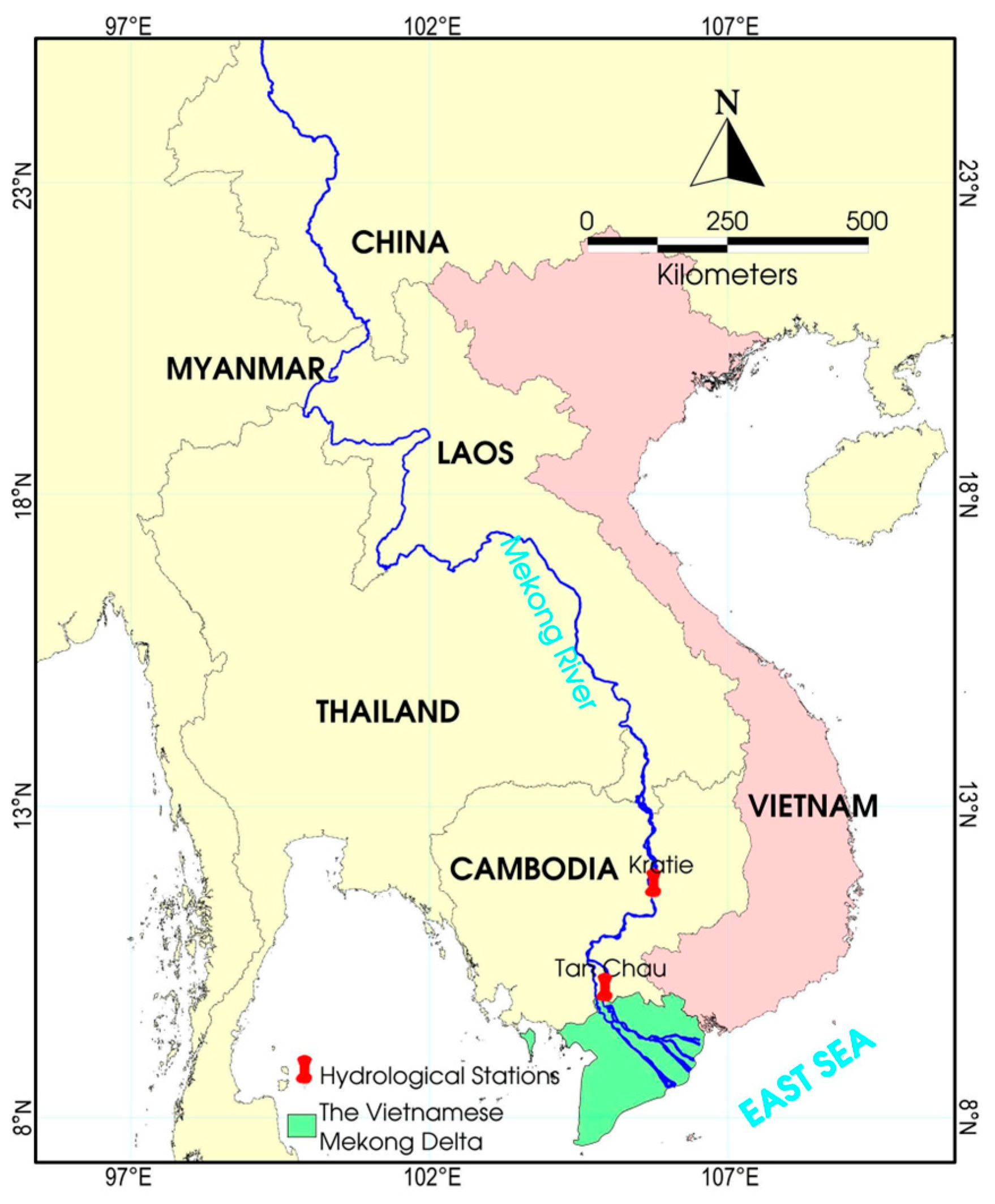
Figure 1. Study area and two hydrological stations (Tan Chau in Viet Nam and Kratie in Cambodia).
Water 18 00923 g001
Figure 2. Time series and box plots of SSC (2009–2023) (a,b) and SF (2009–2021) (c,d) at Tan Chau station, Viet Nam.
Water 18 00923 g002
Figure 3. Temporal variations in water discharge and corresponding box plot at Kratie station for 2009–2023.
Water 18 00923 g003
Figure 4. Random Forest training progress based on OOB error of (a) SC and (b) SF.
Water 18 00923 g004aWater 18 00923 g004b
Figure 5. XGB training curves of (a) SSC and (b) SF.
Water 18 00923 g005
Figure 6. SVM tuning surfaces of (a) sediment concentration and (b) SF.
Water 18 00923 g006
Figure 7. Observed versus predicted SSC (left panels) and SF (right panels) for (a,b) RF, (c,d) XGB, and (e,f) SVM models.
Water 18 00923 g007aWater 18 00923 g007b
Figure 8. RF importance stability for (a) SC and (b) SF.
Water 18 00923 g008
Figure 9. XGB importance stability for (a) SSC and (b) SF.
Water 18 00923 g009aWater 18 00923 g009b
Figure 10. SHAP dependence plots for key discharge variables. (a) Upstream discharge at Kratie (Q_Kratie); (b) mean discharge at Tan Chau (Qmean_TC); and (c) minimum discharge at Tan Chau (Qmin_TC). The y-axis represents the SHAP value, indicating the marginal contribution of each feature to the model’s prediction.
Water 18 00923 g010aWater 18 00923 g010b
Table 1. Summary statistics of variables for predicting SSC (mgL−1).
VariableMinimumMaximumMeanStd. DeviationCoeff. Variation
SSC_TC (mgL−1)0.1557.563.873.71.2
Q_Kratie (m3/s)3209940341123870.7
Hmean_TC (cm)1247914094.10.7
Qmin_TC (m3/s)−626025,60066808942.61.3
Qmean_TC (m3/s)142026,10010,7386769.00.6
Qmax_TC (m3/s)215026,70013,2135515.60.4
Table 2. Summary statistics of variables for predicting SF (tonnes/day).
VariableMinimumMaximumMeanStd. DeviationCoeff. Variation
SF_TC (tonnes/day)71986,42996,553136,5011.4
Q_Kratie (m3/s)4909030359124710.7
Hmean_TC (cm)1640914697.80.7
Qmin_TC (m3/s)−558024,90070058695.71.2
Qmean_TC (m3/s)142025,10010,8056590.20.6
Qmax_TC (m3/s)215025,50012,8815525.70.4
Table 3. Correlation matrix of the data for predicting sediment concentration.
Q_KratieHmean_TCQmin_TCQmean_TCQmax_TCSSC_TC
Q_Kratie1
Hmean_TC0.9801
Qmin_TC0.9640.9281
Qmean_TC0.9480.9160.9891
Qmax_TC0.9040.8840.9460.9681
SSC_TC0.7930.7330.7610.7450.7091
Table 4. Correlation matrix of the data for predicting SF.
Q_KratieHmean_TCQmin_TCQmean_TCQmax_TCSF_TC
Q_Kratie1
Hmean_TC0.9821
Qmin_TC0.9720.9381
Qmean_TC0.9580.9270.9891
Qmax_TC0.9260.9020.9580.9711
SF_TC0.8370.8020.8020.7970.7811
Table 5. Hyperparameter summary.
ModelOptimised Parameter for SSCOptimised Parameter for SF
RFmtrymin_n mtrymin_n
33 53
XGBlearn-ratemin_child_weightmax_depthlearn-ratemin_child_weightmax_depth
0.03160.0516
SVMcostrbf_sigmamargincostrbf_sigmamargin
200.10.1200.20.1
Table 6. Model performances for SC and SF.
ModelSediment ConcentrationSediment Flux
RMSE (mgL−1)R2NSERMSE (tons/Day)R2NSE
RF33.6430.7830.78251,4330.8670.866
XGB34.2660.7740.77455,2360.8470.846
SVM35.1890.7690.76156,8310.8410.837
Disclaimer/Publisher’s Note: The statements, opinions and data contained in all publications are solely those of the individual author(s) and contributor(s) and not of MDPI and/or the editor(s). MDPI and/or the editor(s) disclaim responsibility for any injury to people or property resulting from any ideas, methods, instructions or products referred to in the content.