An Improved Intuitionistic Fuzzy Set TOPSIS Method Based on a New Distance Measure with an Application to Marine Aquaculture Water Quality Evaluation

Abstract

With the rapid development of intensive marine aquaculture, water quality has become a key factor affecting both economic benefits and ecological safety in marine aquaculture. In the process of actual water quality evaluation, due to the great uncertainty and ambiguity of evaluation indicators, experts find it difficult to evaluate in real number form and are more inclined to use linguistic variables to evaluate indicators, which poses challenges for the construction of water quality evaluation models. An intuitionistic fuzzy set (IFS) is an effective tool for dealing with uncertainty and fuzziness in complex problems. Based on a detailed analysis of existing distance measures for IFS, this study proposes a new distance measure that not only considers membership and non-membership information, but also constructs an allocation function for membership and non-membership, introducing hesitation information into distance metrics. We proposed the definitions and proved the properties. The comparative experiments show that the new distance measure can overcome the shortcomings of existing distance measures. Furthermore, based on the newly proposed distance measure, the IFS TOPSIS method is improved in multi-attribute decision-making applications. Finally, a practical application of marine aquaculture water quality evaluation is used. The results illustrate that when $\alpha$ = 1 the closeness declines from 0.741 to 0.432, when =2 the closeness declines from 0.662 to 0.46, and when =6 the closeness declines from 0.566 to 0.82. The convenience and effectiveness of the new method is demonstrated.

1. Introduction

With the rapid development of intensive mariculture, lots of mariculture wastewater containing residual feed and excrement is discharged into marinelands, leading to coastal pollution [1]. Most aquaculture processes require feeding feed, and residual feed and metabolic products of water products produced during aquaculture are some of the main sources of nitrogen and phosphorus pollution in aquaculture systems [2]. The wastewater generated from aquaculture, if discharged directly without purification, will exacerbate the occurrence of red tide. Recently, the environmental problems caused by the discharge of mariculture wastewater have been paid much attention, as have other breeding industries in China [3,4,5,6]. Moreover, the high density of intensive aquaculture often leads to the deterioration of water quality in the later stages of aquaculture, which in turn causes diseases in, or death of, fish and shrimp. So deteriorating water quality has caused massive financial losses to farmers and has become one of the major factors that bottleneck the output and breakage of the production process [7]. Therefore, establishing a method for scientifically evaluating water quality is an important task for culture risk evaluation. Considering the innumerable and complicated variations in water quality (which are often difficult to interpret), monitoring programs and the reliable estimation of water quality play important roles in culture management to provide a thorough understanding of the degree of contamination and to limit its effects [8].

In recent years, due to the complex process of water quality evaluation influenced by multiple indicators and the vague classification boundaries of pollution levels, it is difficult to characterize this uncertainty using traditional methods [9,10,11]. Fuzzy set theory provides a new approach to solving such uncertainty problems. Since Zadeh proposed fuzzy set theory in 1965, various applications based on fuzzy sets have received increasing attention [12]. Fuzzy set (FS) theory reflects the degree of belonging to a certain thing through membership, which is more reasonable than classical set theory when describing fuzziness problems. An enhanced water quality evaluation system was established by Principal Component Analysis/Factor Analysis (PCA/FA), Analytic Hierarchy Process/Entropy Weight Method/Game Theory (AHP/EWM/GT) and Variable Fuzzy Set Theory (VFST). The accuracy of the method was verified by evaluating the water quality of a landfill in a karst area and comparing with the conventional evaluation models [13]. Fang et al. proposed a fuzzy membership model to construct the comprehensive evaluation method of water quality [14]. A new method was developed using a combination of water quality data characteristics and the traditional method of relative membership degree calculation of variable fuzzy sets theory [15]. Considering the influence of temporal and spatial changes on water quality, You et al. proposed an improved fuzzy comprehensive evaluation method for aquaculture water quality evaluation [16]. Current water quality evaluation methods often fail to consider ambiguity and incompleteness with respect to indicator parameters. They may use only membership degree as an evaluation standard, resulting in inaccurate or highly deviated water quality evaluation results. So, it is necessary to develop a new means of water quality evaluation which can describe the uncertainty of indictors comprehensively.

Since FS can effectively depict the fuzzy nature of objective things, research based on fuzzy sets has been widely applied in multi-attribute decision-making, such as map classification, pattern recognition, and other practices since Zadeh proposed FS in 1965 [12]. FS, as proposed by Zadeh, describes ambiguous and indeterminate concepts with indeterminate extensions through membership degrees. Since these FSs can only depict the uncertainty of things through membership degrees, it is difficult to comprehensively describe the fuzziness of things. In 1986, Atanassov [17] proposed the concept of intuitionistic fuzzy sets (IFSs) based on Zadeh’s fuzzy set (FS) theory, representing fuzzy sets with membership functions and non-membership functions, which can simultaneously express information on membership degree, non-membership degree, and hesitation degree. This approach is more flexible and authentic than traditional Zadeh FSs in dealing with conceptual fuzzy uncertainty. According to the characteristics of an IFS, it can not only describe the uncertainty level of fuzzy information but also reflect its unknown degree. Specifically, membership and non-membership indicate the uncertainty level of information, while hesitation reflects the unknown degree of information. The theory of IFSs has thus developed rapidly and become a hot topic of research. In the practice of multi-attribute decision-making, the measurement for IFS information has always been a hot and difficult topic, with distance measures being the most used information measurement tool. Also, it provides a new and effective way to carry out water quality evaluation.

In practical work, we often encounter the problem of comparing two or more fuzzy concepts, which involves comparing the distance between them. In existing methods, the distance measurement for IFSs mainly falls into two aspects: (1) distance for IFSs based on Hamming distance and Euclidean distance; (2) distance for IFSs based on the Hausdorff metric. Atanassov [18] proposed the Hamming distance and Euclidean distance for IFSs based on Zadeh’s FS distance. Bustingce and Burillo proposed the normalized Hamming distance and normalized Euclidean distance [19]. This method only considers membership and non-membership degrees. Wang et al. [20] introduced weights to generalize the Atanassov distance and constructed several distances for IFSs. However, these distances did not consider the hesitation. Szmidt [21] introduced a hesitation degree into Atanassov’s method directly to improve it; subsequently, [22,23] extended the method proposed in [21]. Grzegorzewski [24] and Hung [25] defined the distance for IFSs based on the Hausdorff metric. However, hesitation was not considered in these distance measures. Yang defined the distance for IFSs with the consideration of hesitation directly [26]. Chen et al. proposed an IFS distance formula based on the centroid of a right triangle [27]. However, Shen et al. pointed out certain flaws in [27]. To overcome these flaws, an improved IFS distance formula based on the centroid of a right triangle was proposed [28]. Although both methods consider the level of hesitation in intuitionistic fuzzy numbers, which plays a certain role in measuring the distance between IFSs, and have been applied in practical problems, they still have certain deficiencies in terms of the ability to distinguish the distance between certain intuitionistic fuzzy sets. The distance for IFSs with consideration of width is defined to build quaternary functions [29].

Among the basic information measurement tools for IFSs, either the impact of hesitation is not fully considered, resulting in insufficient differentiation, or the proposed algorithms are difficult to operate, which restricts the application of multi-attribute decision-making. In this study, we propose a new distance measure that not only considers membership and non-membership information, but also constructs an allocation function for membership and non-membership, introducing hesitation information into distance measures. So, we proposed the definitions and proved the properties. The comparative experiments show that the new distance measure can overcome the shortcomings of existing distance measures. Furthermore, based on the newly proposed distance measure, the IFS TOPSIS methods is improved in multi-attribute decision-making applications. Finally, the convenience and effectiveness of the new method is demonstrated through a practical application of marine aquaculture water quality evaluation to illustrate its feasibility and effectiveness.

This paper is organized as follows: In Section 2, we introduce some basic concepts of IFSs, along with definitions and properties of distance measure for IFSs. In Section 3, we analyze the existing distance measures for IFSs in detail. In Section 4, a new distance measure for IFS is proposed, and we compare some existing distance measures for IFSs with the proposed distance measure for IFSs. In Section 5, an improved IFS TOPSIS method based on the proposed distance measure is presented. In Section 6, we apply the proposed method to marine aquaculture water quality evaluation to verify the method. In Section 7, some discussions are presented. In Section 7, finally, we give the conclusion.

2. Preliminary

In this part, we briefly give some concepts of IFSs and operational rules.

Definition 1 

([17]). An IFS $A$ in $X$ is given by

$$A=\{<x,{\mu }_A(x),{\nu }_A(x)|x\in X>\}$$

(1)

where ${\mu }_A(x):X\to [0,1],v_A(x):X\to [0,1]$. With the condition

$$0\le {\mu }_A(x)+{\nu }_A(x)\le 1,\forall x\in X$$

(2)

The numbers ${\mu }_A(x)$, ${\nu }_A(x)\in [0,1]$ denote respectively the degree of membership and non-membership of $x$ to $A$. For convivence, we denote all the IFSs in $X$ by $IFSs(X)$.

$${\pi }_A(x)=1-{\mu }_A(x)-{\nu }_A(x)$$

(3)

For each IFS $A$ in $X$, we identify the intuitionistic index of $x$ in $A$. It is a hesitation degree of $x$ to $A$, and it is obvious that $0\le {\pi }_A\le 1$ for each $x\in X$. Especially, when ${\pi }_A(x)=0$, so ${\mu }_A(x)+{\nu }_A(x)=1$, $A$ degenerates to a Zadeh fuzzy set. Therefore, an IFS can be seen as an extension of a Zadeh FS.

For example, let $A$ be an IFS with membership function ${\mu }_A(x)$ and non-membership function $v_A(x)$ respectively. If ${\mu }_A(x)=0.6$, $v_A(x)=0.3$, then we can get ${\pi }_A(x)=1-0.6-0.3=0.1$. So, it can be interpreted as “the degree that the object $x$ belongs to the intuitionistic fuzzy sets $A$ is 0.6, the degree that the object $x$ doesn’t belong to the intuitionistic fuzzy sets $A$ is 0.3, and the degree of hesitancy is 0.1”.

For convenience’s sake, call $A$ an intuitionistic fuzzy number [19], where

$${\mu }_{\alpha },{\nu }_{\alpha }\in [0,1],0\le {\mu }_{\alpha }+{\nu }_{\alpha }\le 1$$

(4)

Definition 2

([17]). Let $A$, $B$ be intuitionistic fuzzy sets defined in the universe of discourse $X$, where $X=\{x_1,x_2,\dots ,x_n\}$. If $A\subseteq B$, then $\forall x_i\in X$, ${\mu }_A(x_i)\le {\mu }_B(x_i)$ and ${\nu }_A(x_i)\ge {\nu }_B(x_i)$, where $1\le i\le n$.

Definition 3

([26]). Let $D$ be a mapping $D$: $IFSs(X)\times IFSs(X)\to [0,1]$, $D(A,B)$ is said to be a distance for $A\in IFSs(X)$ and $B\in IFSs(X)$, if $D(A,B)$ satisfies the following properties:

(1) 

$0\le D(A,B)\le 1$;

(2) 

$D(A,B)=0$if and only if$A=B$;

(3) 

$D(A,B)=D(B,A)$;

(4) 

if $A\subseteq B \subseteq C$, $A,B,C\in IFSs(X)$, then $D(A,C)\ge D(A,B)$ and $D(A,C)\ge D(B,C)$.

3. Analysis of Distance Measures for IFSs

To simplify the formula for representing the distance for IFSs, this study uses the following symbols for abbreviation. Let $A$, $B$ be intuitionistic fuzzy sets defined in the universe of discourse $X$, where $X=\{x_1,x_2,\dots ,x_n\}$. Note ${\Delta }_{\mu }^{AB}(i)={\mu }_A(x_i)-{\mu }_B(x_i)$, ${\Delta }_{\nu }^{AB}(i)={\nu }_A(x_i)-{\nu }_B(x_i)$, and ${\Delta }_{\pi }^{AB}(i)={\pi }_A(x_i)-{\pi }_B(x_i)$ respectively represent the difference in membership between two IFSs $A$ and $B$, as well as the difference in non-membership and hesitation.

3.1. Hamming Distance and Euclidean Distance for IFSs

Let $A=\{<x_i,{\mu }_A(x_i),{\nu }_A(x_i)>|x_i\in X\}$, $B=\{<x_i,{\mu }_B(x_i),{\nu }_B(x_i)>|x_i\in X\}$ be two IFSs. Based on Zadeh’s fuzzy distance measure, Atanassov [18] proposed Hamming distance $H{D}_{Ata}(A,B)$ and Euclidean distance $E{D}_{Ata}(A,B)$ as follows:

$$H{D}_{Ata}(A,B)={\displaystyle \frac{1}{2}}{\displaystyle \sum _{i=1}^n|{\Delta }_{\mu }^{AB}}(i)|+|{\Delta }_{\nu }^{AB}(i)|$$

(5)

$$E{D}_{Ata}(A,B)=\sqrt{{\displaystyle \frac{1}{2}}{\displaystyle \sum _{i=1}^n|{\Delta }_{\mu }^{AB}}(i){|}^2+|{\Delta }_{\nu }^{AB}(i){|}^2}$$

(6)

Bustince and Burillo [19] proposed the normalized Hamming distance and normalized Euclidean distance as follows:

$$NH{D}_{BB}(A,B)={\displaystyle \frac{1}{2n}}{\displaystyle \sum _{i=1}^n|{\Delta }_{\mu }^{AB}}(i)|+|{\Delta }_{\nu }^{AB}(i)|$$

(7)

$$NE{D}_{BB}(A,B)=\sqrt{{\displaystyle \frac{1}{2n}}{\displaystyle \sum _{i=1}^n|{\Delta }_{\mu }^{AB}}(i){|}^2+|{\Delta }_{\nu }^{AB}(i){|}^2}$$

(8)

Despite there being a linear relationship between hesitation, membership, and non-membership as in Equation (3), we can still get the following results:

$${\Delta }_{\pi }^{AB}(i)\ne |{\Delta }_{\mu }^{AB}(i)+{\Delta }_{\nu }^{AB}(i)|$$

(9)

$${({\Delta }_{\pi }^{AB}(i))}^2\ne |{({\Delta }_{\mu }^{AB}(i))}^2+{({\Delta }_{\nu }^{AB}(i))}^2|$$

(10)

Therefore, if ${\Delta }_{\pi }^{AB}(i)$ and ${({\Delta }_{\pi }^{AB}(i))}^2$ are directly introduced into Hamming distance and Euclidean distance measures, the distance measure results undergo essential changes. So, hesitation cannot be ignored in the distance measures of IFSs. Szmidt and Kacprzyk [23] proposed improved Hamming distance and Euclidean distance as follows:

$$H{D}_{SK}(A,B)={\displaystyle \frac{1}{2}}{\displaystyle \sum _{i=1}^n|{\Delta }_{\mu }^{AB}}(i)|+|{\Delta }_{\nu }^{AB}(i)|+|{\Delta }_{\pi }^{AB}(i)|$$

(11)

$$NH{D}_{SK}(A,B)={\displaystyle \frac{1}{2n}}{\displaystyle \sum _{i=1}^n|{\Delta }_{\mu }^{AB}}(i)|+|{\Delta }_{\nu }^{AB}(i)|+|{\Delta }_{\pi }^{AB}(i)|$$

(12)

$$E{D}_{SK}(A,B)=\sqrt{{\displaystyle \frac{1}{2}}{\displaystyle \sum _{i=1}^n|{\Delta }_{\mu }^{AB}}(i){|}^2+|{\Delta }_{\nu }^{AB}(i){|}^2+|{\Delta }_{\pi }^{AB}(i){|}^2}$$

(13)

$$NE{D}_{SK}(A,B)=\sqrt{{\displaystyle \frac{1}{2n}}{\displaystyle \sum _{i=1}^n|{\Delta }_{\mu }^{AB}}(i){|}^2+|{\Delta }_{\nu }^{AB}(i){|}^2+|{\Delta }_{\pi }^{AB}(i){|}^2}$$

(14)

From (11) to (14), the IFS is represented in three-dimensional coordinate $<{\mu }_i,{\nu }_i,{\pi }_i>$. So, the distance measure proposed by Szmidt and Kacprzyk essentially represents the two three-dimensional vectors, specifically the distance metric between $({\mu }_A(x_i),{\nu }_A(x_i),{\pi }_A(x_i))$ and $({\mu }_B(x_i),{\nu }_B(x_i),{\pi }_B(x_i))$. Therefore, it satisfies Property 1 to 3 in Definition 3. However, directly incorporating the hesitation difference ${\Delta }_{\pi }^{AB}(i)$ into the distance metric may not necessarily satisfy Property 4. Let us conduct a detailed analysis of this.

Let $A$, $B$, $C$ be IFSs defined in the universe of discourse $X$, where $X=\{x_1,x_2,\dots ,x_n\}$.

From Definitions 2 and 3, we can see that if $A$, $B$ and $C$ satisfy $A\subseteq B \subseteq C$, then the corresponding membership degree and non-membership degree satisfy ${\mu }_A(x_i)\le {\mu }_B(x_i)\le {\mu }_C(x_i)$ and ${\nu }_A(x_i)\ge {\nu }_B(x_i)\ge {\nu }_C(x_i)$. This leads to the following conclusion:

$${\Delta }_{\mu }^{AC}(i)\le {\Delta }_{\mu }^{AB}(i)\le 0, {\Delta }_{\nu }^{AC}(i)\ge {\Delta }_{\nu }^{AB}(i)\ge 0$$

(15)

$$|{\Delta }_{\mu }^{AB}(i)|\le |{\Delta }_{\mu }^{AC}(i)|, |{\Delta }_{\nu }^{AB}(i)|\le |{\Delta }_{\nu }^{AC}(i)|$$

(16)

As the relationship between hesitation and membership as well as non-membership is shown in Equation (3), then we can get the following result:

$$|{\Delta }_{\pi }^{AB}(i)|=|{\Delta }_{\mu }^{AB}(i)+{\Delta }_{\nu }^{AB}(i)|$$

(17)

$$|{\Delta }_{\pi }^{AC}(i)|=|{\Delta }_{\mu }^{AC}(i)+{\Delta }_{\nu }^{AC}(i)|$$

(18)

From Equation (18) we can find that $|{\Delta }_{\pi }^{AC}(i)|\ge |{\Delta }_{\pi }^{AB}(i)|$ may not necessarily hold true. This leads to Equations (19)–(22) that follow not necessarily holding true.

$$H{D}_{SK}(A,B)\le H{D}_{SK}(A,C)$$

(19)

$$NH{D}_{SK}(A,B)\le NH{D}_{SK}(A,C)$$

(20)

$$E{D}_{SK}(A,B)\le E{D}_{SK}(A,C)$$

(21)

$$NE{D}_{SK}(A,B)\le E{D}_{SK}(A,C)$$

(22)

So Equations (11)–(14) cannot satisfy Property 4 in Definition 3.

From the above analysis, it can be seen that if IFS $A$, $B$ and $C$ satisfy $A\subseteq B \subseteq C$, then the relationship between $|{\Delta }_{\pi }^{AC}(i)|$ and $|{\Delta }_{\pi }^{AB}(i)|$ cannot be determined. Therefore, directly constructing hesitation differences into three-dimensional space in the distance measure can lead to contradictions in Property 4 of Definition 3.

3.2. Hausdorff Distance for IFS

With respect to the Hausdorff distance, Grzegorzewski [24] and Hung [25] proposed definitions for IFSs as follows. They are generalizations of Hamming distance and Euclidean distance.

$$H{D}_{GH}(A,B)={\displaystyle \sum _{i=1}^n\max (|{\Delta }_{\mu }^{AB}}(i)|,|{\Delta }_{\nu }^{AB}(i)|)$$

(23)

$$NH{D}_{GH}(A,B)={\displaystyle \frac{1}{n}}{\displaystyle \sum _{i=1}^n\max (|{\Delta }_{\mu }^{AB}}(i)|,|{\Delta }_{\nu }^{AB}(i)|)$$

(24)

$$E{D}_{GH}(A,B)=\sqrt{{\displaystyle \sum _{i=1}^n\max (|{\Delta }_{\mu }^{AB}}(i){|}^2,|{\Delta }_{\nu }^{AB}(i){|}^2)}$$

(25)

$$NE{D}_{GH}(A,B)=\sqrt{{\displaystyle \frac{1}{n}}{\displaystyle \sum _{i=1}^n\max (|{\Delta }_{\mu }^{AB}}(i){|}^2,|{\Delta }_{\nu }^{AB}(i){|}^2)}$$

(26)

Yang [26] proposed a three-dimensional distance measure with a consideration of hesitation directly, as follows.

$$H{D}_{Ya}(A,B)={\displaystyle \sum _{i=1}^n\max (|{\Delta }_{\mu }^{AB}}(i)|,|{\Delta }_{\nu }^{AB}(i)|,|{\Delta }_{\pi }^{AB}(i)|)$$

(27)

$$NH{D}_{Ya}(A,B)={\displaystyle \frac{1}{n}}{\displaystyle \sum _{i=1}^n\max (|{\Delta }_{\mu }^{AB}}(i)|,|{\Delta }_{\nu }^{AB}(i)|,|{\Delta }_{\pi }^{AB}(i)|)$$

(28)

$$E{D}_{Ya}(A,B)=\sqrt{{\displaystyle \sum _{i=1}^n\max (|{\Delta }_{\mu }^{AB}}(i){|}^2,|{\Delta }_{\nu }^{AB}(i){|}^2,|{\Delta }_{\pi }^{AB}(i){|}^2)}$$

(29)

$$NE{D}_{Ya}(A,B)=\sqrt{{\displaystyle \frac{1}{n}}{\displaystyle \sum _{i=1}^n\max (|{\Delta }_{\mu }^{AB}}(i){|}^2,|{\Delta }_{\nu }^{AB}(i){|}^2,|{\Delta }_{\pi }^{AB}(i){|}^2)}$$

(30)

Based on the previous analysis, we can get that if IFS $A$, $B$ and $C$ satisfy $A\subseteq B \subseteq C$, then the relationship between $|{\Delta }_{\pi }^{AC}(i)|$ and $|{\Delta }_{\pi }^{AB}(i)|$ cannot be determined. So, Equations (27)–(30) cannot satisfy Property 4 in Definition 3.

Wang combined Hamming distance and Hausdorff distance, with a distance measure proposed as follows:

$$D_{Wa}(A,B)={\displaystyle \frac{1}{n}}{\displaystyle \sum _{i=1}^n\left[\frac{|{\Delta }_{\mu }^{AB}(i)|+|{\Delta }_v^{AB}(i)|}{4}+\frac{\max (|{\Delta }_{\mu }^{AB}(i)|,|{\Delta }_v^{AB}(i)|)}{2}\right]}$$

(31)

Hesitation was not considered in Equation (31).

In summary, the existing distance measurement methods for IFSs primarily combine Hamming, Euclidean, and Hausdorff distances. They are constructed using the absolute value or square of the difference in membership, the difference in non-membership, or the difference in hesitation between two intuitionistic fuzzy sets. Some of these methods only consider the differences in membership and non-membership, ignoring the impact of the difference in hesitation on distance. While others simultaneously consider the three elements of membership difference, non-membership difference, and hesitation difference in distance measurement, due to the special status of hesitation in IFS distances (which is different from the status of membership degrees and non-membership in IFSs), the difference in hesitation is directly introduced into IFSs like the difference in membership and non-membership, often resulting in insufficient discriminative ability. Although the assignment of hesitation has been considered in research, the adoption of an average assignment method overlooks the distinct impacts of membership and non-membership on the distribution of hesitation.

Since both membership and non-membership reflect the degree of uncertainty of information, and the membership (non-membership) clearly depicts the extent to which an element belongs (does not belong) to an uncertain object, they have the same status and role in IFSs. However, hesitation degree reflects the degree of unknowingness of information, which can be interpreted as the degree of ambiguity in a decision-maker’s affirmation or denial of an uncertain object. Therefore, hesitation may contain a degree of partial affirmation, and it may also contain a degree of partial denial. If further explanation or clarification is provided for uncertain objects, the degree of hesitation may be partially or fully converted into membership degree (or non-membership degree). In this sense, the status and role of hesitation degree, membership degree, and non-membership in IFS cannot be treated equally, and hesitation degree has a certain degree of allocation to membership degree and non-membership degree with different weight.

4. A New Distance Measure for IFSs

From the analysis in the above section, we can get that membership and non-membership describe the degree of uncertainty for fuzzy information in IFSs, while hesitation describes the degree of ambiguity. Therefore, the role of hesitation, membership and non-membership in IFSs cannot be treated equally. Therefore, any result obtained by directly introducing hesitation into the distance measure will not satisfy Property 4 in Definition 3. This indicates that the introduction of hesitation cannot be simply equated with the introduction of membership or non-membership in distance measures. Let $A$ be an IFS defined in the universe of discourse $X$, where $X=\{x_1,x_2,\dots ,x_n\}$. It represents the voting of n experts on decision-making scheme $A$. The level of support from Expert $x_i$ for A is expressed as ${\mu }_A(x_i)$, degree of opposition is expressed as ${\nu }_A(x_i)$, and degree of abstention is expressed as ${\pi }_A(x_i)$. If ${\mu }_A(x_i)$ = 0.6, ${\nu }_A(x_i)$ = 0.1, so ${\pi }_A(x_i)$ = 0.3. If, after some persuasion, he may change his entire abstention to support, then the best outcome would be ${\mu }_{A+final}(x_i)=0.6+0.3=0.9$, ${\nu }_A(x_i)$ = 0.1. On the contrary, if he changes the degree of abstention entirely to the opposing part, the result would be ${\nu }_{A+final}(x_i)=0.1+0.3=0.4$ ${\mu }_A(x_i)$ = 0.6. Of course, there are also cases where a portion of the abstention will be voted in favor of, while another portion will be voted against. After some persuasion, support from Expert $x_i$ for A could be any number between 0.6 and 0.9, and degree of opposition could be any number between 0.1 and 0.4. Simultaneously, the condition must be met: ${\mu }_{A+final}(x_i)+{\nu }_{A+final}(x_i)=1$; we called this hesitation allocation. Considering the herd mentality of those who abstain, the difference in the proportion of those who support and oppose will subtly influence the inclination of those who are hesitant. When the number of supporters exceeds the number of opponents, the abstainers are more likely to lean towards support, and vice versa. We can get that membership and non-membership not only have an impact on the distribution of hesitation, but also have their weights. Therefore, based on this idea, this study proposes a new distance measure for IFSs.

4.1. Gaussian Weight Construction

4.1.1. Definition of Gaussian Weight

The Gaussian function (and its derived Sigmoid form) exhibits smoothness and nonlinearity. Compared to linear assignment, the Gaussian function is more sensitive to changes in distance and is differentiable everywhere, which is crucial in optimization and derivation proofs. The Sigmoid form is commonly used in machine learning and artificial neural networks as a nonlinear activation function. It plays a significant role in nonlinearly transforming raw data, amplifying and highlighting the differences between feature data, and is essential in various tasks such as classification, regression, and time series prediction.

Definition 4.

Let$A$be an IFS defined in the universe of discourse$X$, where$X=\{x_1,x_2,\dots ,x_n\}$. So we can get hesitation based on Equation (3). We can also get the Euclidean distance of IFS A to the two ideal points$P_{ture}(1,0)$and$P_{false}(0,1)$as follows:

$$D_{true}^2(A(x_i))={(1-{\mu }_A(x_i))}^2+{\nu }_A{(x_i)}^2$$

(32)

$$D_{false}^2(A(x_i))={\mu }_A{(x_i)}^2+{(1-{\nu }_A(x_i))}^2$$

(33)

Based on this, we proposed the allocation weight of membership${\omega }_{\mu }(A(x_i))$and non-membership ${\omega }_{\nu }(A(x_i))$respectively, as follows:

$${\omega }_{\mu }(A(x_i))={\displaystyle \frac{\exp (-\frac{D_{true}^2(A(x_i))}{2{\sigma }^2})}{\exp (-\frac{D_{true}^2(A(x_i))}{2{\sigma }^2})+\exp (-\frac{D_{false}^2(A(x_i))}{2{\sigma }^2})}}$$

(34)

$${\omega }_{\nu }(A(x_i))=1-{\omega }_{\mu }(A(x_i))$$

(35)

where $\sigma$ is the kernel width parameter, which can be set as a constant.

By substituting $D_{true}^2(A(x_i))$, $D_{false}^2(A(x_i))$ and simplifying, we can obtain the Sigmoid form as follows:

$${\omega }_{\mu }(A(x_i))={\displaystyle \frac{1}{1+\exp (-\frac{{\mu }_A(x_i)-{\nu }_A(x_i)}{{\sigma }^2})}}$$

(36)

$${\omega }_{\nu }(A(x_i))=1-{\omega }_{\mu }(A(x_i))$$

(37)

This method utilizes the Gaussian kernel function to smoothly and reasonably allocate “hesitant” information to either “support” or “oppose” based on the current “support/oppose” trend, thereby constructing an advanced distance measure that satisfies strict monotonicity mathematically and aligns with human intuition in a physical sense. It can enhance distinguishability on sets with minimal differences and holds significant importance for distance measures for IFSs.

4.1.2. Theoretical Basis for Positive Real Number Constraint of the Kernel Width Parameter

Definition 5. 

Kernel width parameter$\sigma$is strictly defined as a positive real number; that is, $\sigma \in {\mathbb{R}}^{+}=\{\sigma \mid \sigma >0\}$.

This constraint is based on the following three theoretical principles:

1. 

Mathematical well-definedness

In Equation (37), the exponential term $\exp (-{\displaystyle \frac{{\mu }_A(x_i)-{\nu }_A(x_i)}{{\sigma }^2}})$ needs to be examined.

If $\sigma =0$:

• • when ${\mu }_A(x_i)\ne {\nu }_A(x_i)$,${\displaystyle \frac{{\mu }_A(x_i)-{\nu }_A(x_i)}{{\sigma }^2}}\to \pm \infty$, this leads to divergence of$\exp (\pm \infty )$.
  • ${\omega }_{\mu }(A(x_i))$ degenerates into a discontinuous step function, as follows:

    $${\omega }_{\mu }(A(x_i))=\left\{\begin{array}{c}0,{\mu }_A(x_i)<{\nu }_A(x_i)\\ undefined,{\mu }_A(x_i)={\nu }_A(x_i)\\ 1,{\mu }_A(x_i)>{\nu }_A(x_i)\end{array}\right.$$

    (38)

If $\sigma <0$:

• • Although  ${\sigma }^2>0$ makes the function formally defined, it violates the physical semantics of the parameters.

2. 

Unification of Gaussian Kernel Theory

In Kernel Methods theory, Gaussian kernel is also known as Radial Basis Function Kernel (RBF Kernel) and its standard form is shown as follows:

$$K(x,y)=\mathrm{e}\mathrm{x}\mathrm{p}(-{\displaystyle \frac{\parallel x-y{\parallel }^2}{2{\sigma }^2}})$$

(39)

$$\sigma =\sqrt{\mathbb{E}\left[\right(X-\mu {)}^2]}\ge 0$$

(40)

where$\sigma$ is bandwidth. In statistics, it corresponds to the standard deviation of a normal distribution. The definition requirement of standard deviation is as follows:

• only when the random variable degenerates to a constant $\sigma =0$. In the non-degenerate case, it must hold that $\sigma >0$.

The Sigmoid form of this study can be regarded as a transformation of the Gaussian kernel, so it inherits the requirement of the Gaussian kernel for $\sigma >0$.

3. 

Physical Interpretability

In signal processing and machine learning, $\sigma$controls the “smoothness” or “sensitivity” of the function.

• • The smaller $\sigma$ is, the more sensitive the function is to input changes (high-frequency response);
  • The larger $\sigma$ is, the more insensitive the function is to input changes (low-frequency response).

As a geometric quantity, “width” does not have a negative value in the physical world. A negative $\sigma$ will lead to “inverse smoothing”, which can be mathematically defined but is uninterpretable in terms of application semantics.

4.1.3. Derivation of Kernel Width Parameter Values Based on Data Precision of IFSs

In practical applications of IFSs, membership and non-membership are typically represented with finite precision. This accuracy constraint imposes clear requirements on the design of the weight function:

• Input accuracy: $\mu ,\nu$ retain two decimal places; that is, $\mu ,\nu \in \left\{0.00,0.01,0.02,\dots ,0.99,1.00\right\}$;
• Smallest discernible difference: ${\Delta }_{\min }=\min \{\left|\mu -\nu \right|:\mu \ne \nu \}=0.01$;
• Output accuracy requirements: ${\omega }_{\mu }$ should be rounded to three decimal places, with an accuracy one order of magnitude higher than the input, to avoid information loss.

1.

Definition of effective working range

Definition 6

(Effective working range). Let $A$ be an IFS defined in the universe of discourse $X$, where $X=\{x_1,x_2,\dots ,x_n\}$. Let ${\omega }_{\mu }(x_i)\in {\omega }_{valid}$ denote the effective working range, where ${\omega }_{valid}=\left[0.001,0.499\right]\cup \left[0.501,0.999\right]$.

This interval excludes three types of degenerate situations shown in

Table 1. Three types of degenerate situations.

Degenerate Situations	Interval	Consequence
Extreme saturation	$[0.0,0.001)\cup (0.999,1]$	Weight tends to be hard 0/1, gradient vanishing, loss of differentiability
Precision blind spot	$(0.499,0.501)$	When the weight is rounded to three decimal places, it is impossible to distinguish between $\mu (x_i)>\nu (x_i)$ and $\mu (x_i)<\nu (x_i)$

Note: Semantic interpretation.

.

• ${\omega }_{\mu }\in \left[0.001,0.499\right]\leftrightarrow \nu$ dominates ($\mu (x_i)<\nu (x_i)$). The membership weight is reasonably suppressed;
• ${\omega }_{\mu }\in \left[0.501,0.999\right]\leftrightarrow \mu$ dominates ($\mu (x_i)>\nu (x_i)$). The membership weight is reasonably increased;
• ${\omega }_{\mu }\approx 0.5\leftrightarrow$ completely neutral state ($\mu (x_i)\approx \nu (x_i)$). However, it should be avoided under limited precision.

2.

Theorem and proof

Theorem 1

(necessary range of values for the kernel width parameter). Let $A$ be an IFS defined in the universe of discourse $X$, where $X=\{x_1,x_2,\dots ,x_n\}$.

Let $\Delta (i)={\mu }_A(x_i)-{\nu }_A(x_i)$ be the difference of membership and non-membership, which satisfies $\left|\Delta (i)\right|\in \left|{\Delta }_{\min },{\Delta }_{\max }\right|=[0.01,1.00]$. For Gaussian Weight function

$${\omega }_{\mu }(\Delta (i))={\displaystyle \frac{1}{1+\exp (-\frac{\Delta (i)}{{\sigma }^2})}}$$

(41)

the range of values for the kernel width parameter $\sigma$ is

$$\sigma \in [{\displaystyle \frac{1}{\sqrt{\ln 999}}},\sqrt{{\displaystyle \frac{{\Delta }_{\min }}{\ln (501/499)}}}]\approx \left[0.380,1.581\right]$$

(42)

when $\left|\Delta (i)\right|\in \left|{\Delta }_{\min },{\Delta }_{\max }\right|$ satisfies ${\omega }_{\mu }(\Delta (i))\in {\omega }_{valid}$. The proof is shown in Appendix A.

4.2. Hesitation Allocation Function Constructing

Based on the allocation weight of membership ${\omega }_{\mu }(A(x_i))$ and non-membership ${\omega }_{\nu }(A(x_i))$,we proposed a hesitation allocation function.

Definition 7. 

(1) Allocation function of membership to hesitation is as follows:

$$M_{\pi \to \mu }({\mu }_A(x_i),{\nu }_A(x_i))={\mu }_A(x_i)+{\omega }_{\mu }(A(x_i))•{\pi }_A(x_i)$$

(43)

(2) Allocation function of non-membership to hesitation is as follows:

$$M_{\pi \to \nu }({\mu }_A(x_i),{\nu }_A(x_i))={\nu }_A(x_i)+{\omega }_{\nu }(A(x_i))•{\pi }_A(x_i)$$

(44)

It is obvious that$M_{\pi \to \mu }({\mu }_A(x_i),{\nu }_A(x_i))+M_{\pi \to \nu }({\mu }_A(x_i),{\nu }_A(x_i))=1$. So, a four-dimensional form of$A$is constructed as follows:

$$A=\left({\mu }_A(x_i),{\nu }_A(x_i),M_{\pi \to \nu }({\mu }_A(x_i),{\nu }_A(x_i)),M_{\pi \to \mu }(({\mu }_A(x_i),{\nu }_A(x_i))\right)$$

(45)

4.3. A New Type of Distance Measure for IFSs

Let $A$ be an IFS defined in the universe of discourse $X$, where $X=\{x_1,x_2,\dots ,x_n\}$. The four-dimensional form consisting of ${\mu }_A(x_i)$, ${\nu }_A(x_i)$, $M_{\pi \to \mu }({\mu }_A(x_i),{\nu }_A(x_i))$, and $M_{\pi \to \nu }({\mu }_A(x_i),{\nu }_A(x_i))$ with each element $x_i$ is a point in the four-dimensional real number space.

Definition 8. 

Let$A=\{<x_i,{\mu }_A(x_i),{\nu }_A(x_i)|x_i\in X>\}$ and $B=\{<x_i,{\mu }_B(x_i),{\nu }_B(x_i)|x_i\in X>\}$ be two IFSs in $X=\{x_1,x_2,\dots ,x_n\}$. They are two points in the four-dimensional real number space, so the distance between IFS$A$ and $B$is defined as follows:

$$D(A,B)=\sqrt{{\displaystyle \frac{1}{4}}\left[{\left|{\Delta }_{\mu }^{AB}\right|}^2+{\left|{\Delta }_{\nu }^{AB}\right|}^2+{\left|{\Delta }_{\pi \to \mu }^{AB}\right|}^2+{\left|{\Delta }_{\pi \to \nu }^{AB}\right|}^2\right]}$$

(46)

where

• ${\Delta }_{\mu }^{AB}(i)={\mu }_A(x_i)-{\mu }_B(x_i)$,
• ${\Delta }_{\nu }^{AB}(i)={\nu }_A(x_i)-{\nu }_B(x_i)$,
• ${\Delta }_{\pi \to \mu }^{AB}(i)=M_{\pi \to \mu }({\mu }_A(x_i),{\nu }_A(x_i))-M_{\pi \to \mu }({\mu }_B(x_i),{\nu }_B(x_i))$,
• ${\Delta }_{\pi \to \nu }^{AB}(i)=M_{\pi \to \nu }({\mu }_A(x_i),{\nu }_A(x_i))-M_{\pi \to \nu }({\mu }_B(x_i),{\nu }_B(x_i))$.

Theorem 2

([26]). Let $A$, $B$, $C$ be IFSs defined in the universe of discourse X. $D(A,B)$ is said to be a distance measure for IFS $A$ and IFS $B$, which $D(A,B)$ satisfies in the following properties:

(1) 

$0\le D(A,B)\le 1$;

(2) 

$D(A,B)=0$if and only if$A=B$;

(3) 

$D(A,B)=D(B,A)$;

(4) 

if$A\subseteq B \subseteq C$,$A,B ,C\in IFSs(X)$, then$D(A,C)\ge D(A,B)$ and $D(A,C)\ge D(B,C)$.

The proof of Theorem 2 for Equation (46) is shown in Appendix B.

Let $A=\{<x_i,{\mu }_A(x_i),{\nu }_A(x_i)|x_i\in X>\}$ and $B=\{<x_i,{\mu }_B(x_i),{\nu }_B(x_i)|x_i\in X>\}$ be two IFSs in $X=\{x_1,x_2,\dots ,x_n\}$. Based on Equation (44) and the Minkowski distance measure in real number space, we can define the Minkowski distance for $A$ and $B$.

Definition 9.

Let $A=\{<x_i,{\mu }_A(x_i),{\nu }_A(x_i)|x_i\in X>\}$ and $B=\{<x_i,{\mu }_B(x_i),{\nu }_B(x_i)|x_i\in X>\}$ be two IFSs in $X=\{x_1,x_2,\dots ,x_n\}$. They are two points in the four-dimensional real number space and based on Equation (46), so the distance between A and B is defined as follows:

$$NMD(A,B)={\left[{\displaystyle \frac{1}{4n}}{\displaystyle \sum _{i=1}^n\left[{\left|{\Delta }_{\mu }^{AB}\right|}^{\alpha }+{\left|{\Delta }_{\nu }^{AB}\right|}^{\alpha }+{\left|{\Delta }_{\pi \to \mu }^{AB}\right|}^{\alpha }+{\left|{\Delta }_{\pi \to \nu }^{AB}\right|}^{\alpha }\right]}\right]}^{1/\alpha }$$

(47)

where $1\le \alpha <+\infty$. From the proof of Equation (46) in Appendix B, following the same reasoning, we can prove Equation (47) satisfies the properties in Theorem 2.

If ${\pi }_A(x_i)={\pi }_B(x_i)=0$, then IFS A and B degenerate into FSs, so for the distance proposed in this study, $NM{D}^{\alpha }(A,B)$:

If $\alpha =1$, then $NM{D}^{\alpha }(A,B)=NH{D}_{FS}(A,B)$;

If $\alpha =2$, $NM{D}^{\alpha }(A,B)=NE{D}_{FS}(A,B)$

So, the proposed distance measure in this study is a generalization of the Zadeh FS distance measure.

4.4. Comparison of Distance Measures for IFSs

We adopt some cases of IFSs used in [29] to compare the results of proposed distance measures with existing distance measures, and the results are shown in Table 2.

(1) In some situations, the existing distance measures cannot make distinctions due to the same results. For example, in case 2, if voting is used, it can be interpreted as: if 10 people vote, {<x, (1, 0)>} indicates that everyone agrees, {<x, (0.5, 0.5)>} indicates that five people agree and five disagree, and {<x, (0, 0)>} indicates that everyone abstains. So, it is reasonable to believe that there is a difference in the distance for {<x, (1, 0)>} and {<x, (0, 0)>} and in the distance for {<x, (0.5, 0.5)>} and {<x, (0, 0)>}. But in the existing distance measure, $H{D}_{Ata}$, $E{D}_{Ya}$ and $H{D}_{SK}$ have the same results, as they treat the roles of membership, non-membership and hesitation equally. For example, in case 1, $H{D}_{Ata}$, $E{D}_{Ata}$, $H{D}_{GH}$ and $E{D}_{GH}$ have the same results because they have the same results in terms of hesitation difference. For the same reason, in case 3, $H{D}_{GH}$ and $E{D}_{GH}$ have the same results.

(2) In some situations, the existing distance measure gets the wrong results. For example, in case 1, we can get {<x, (0.3, 0.4)>} $\subset$ {<x, (0.3, 0.3)>}, {<x, (0.4, 0.4)>} $\subset$ {<x, (0.4, 0.3)>}. Based on Definition 3, the distance for {<x, (0.3, 0.3)>} and {<x, (0.4,0.4)>} is less than the distance for {<x, (0.3, 0.4)>} and {<x, (0.4, 0.3)>}. But $H{D}_{SK}$, $E{D}_{Ya}$ and $E{D}_{SK}$ get the wrong result.

We adopt some cases of IFSs used in [30] for pattern recognition. Let $P_1$, $P_2$ be IFSs defined in the universe of discourse $X=\{x_1,x_2,x_3\}$ respectively, where

$$\begin{gathered} P_1=\left\{<x_1, \left(0.6,0.25\right)>,<x_2, \left(0,0.25\right)>,<x_3, \left(0.3,0.25\right)>\right\} \\ P_2=\left\{<x_1, \left(0.1,0.75\right)>,<x_2, \left(0.15,0.1\right)>,<x_3, \left(0.2,0.35\right)>\right\} \end{gathered}$$

We want to classify an unknown pattern represented by IFS $Q$ into one of the patterns, $P_1$ or $P_2$, where

$$Q=\left\{<x_1, \left(0,0.15\right)>,<x_2, \left(0.325,0.425\right)>,<x_3, \left(0.2,0.25\right)>\right\}$$

Let ${\omega }_i$ be the weight of $x_i$, where ${\omega }_i={\displaystyle \frac{1}{3}}$ and $1\le i\le 3$.

From Table 3, we can get that the distance measure $D_{CC}$ proposed in [30] cannot be determined as $D_{CC}(P_1,Q)$ = 0.1278, $D_{CC}(P_2,Q)$ = 0.1278. We can also get $NM{D}^1(proposed)(P_1,Q)$ > $NM{D}^1(proposed)(P_2,Q)$, $NM{D}^2(proposed)(P_1,Q)$ > $NM{D}^2(proposed)(P_2,Q)$ and $NM{D}^6(proposed)(P_1,Q)$ > $NM{D}^6(proposed)(P_2,Q)$. Then the unknown pattern represented by IFS $Q$ is classified into pattern $P_2$. The result coincides with the result in [28].

Table 2. Comparison of distance measures for IFS A and B.

Distance Measures	Case 1		Case 2		Case 3
	A = <x, 0.3, 0.3> B = <x, 0.4, 0.4>	A = <x, 0.3, 0.4> B = <x, 0.4, 0.3>	A = <x, 1, 0> B =<x, 0, 0>	A = <x, 0.5, 0.5> B = <x, 0, 0>	A = <x, 0.4, 0.2> B = <x, 0.5, 0.3>	A = <x, 0.4, 0.2> B = <x, 0.5, 0.2>
$H{D}_{Ata}$ [20]	0.1000	0.1000	0.5000	0.5000	0.1000	0.0500
$E{D}_{Ata}$ [20]	0.1000	0.1000	0.7071	0.5000	0.1000	0.7007
$H{D}_{SK}$ [23]$, E{D}_{Ya}$ [13]	0.2000	0.1000	1.0000	1. 0000	0.2000	0.1000
$E{D}_{SK}$ [23]	0.1732	0.1000	1.0000	0.8660	0.1732	0.1000
$H{D}_{GH}$ [26,27]	0.1000	0.1000	1.0000	0.5000	0.1000	0.1000
$E{D}_{GH}$ [26,27]	0.1000	0.1000	1.0000	0.5000	0.1000	0.1000
$NM{D}^1(proposed)$	0.0500	0.1757	0.5000	0.2500	0.0902	0.0394
$NM{D}^2(proposed)$	0.0710	0.1913	0.6124	0.3536	0.0908	0.0540
$NM{D}^6(proposed)$	0.0900	0.2241	0.7978	0.4454	0.0927	0.0794

Notes: The gray background color denotes results that do not make distinctions due to the same results. The orange background color denotes wrong results.

Table 2. Comparison of distance measures for IFS A and B.

Distance Measures	Case 1		Case 2		Case 3
	A = <x, 0.3, 0.3> B = <x, 0.4, 0.4>	A = <x, 0.3, 0.4> B = <x, 0.4, 0.3>	A = <x, 1, 0> B =<x, 0, 0>	A = <x, 0.5, 0.5> B = <x, 0, 0>	A = <x, 0.4, 0.2> B = <x, 0.5, 0.3>	A = <x, 0.4, 0.2> B = <x, 0.5, 0.2>
$H{D}_{Ata}$ [20]	0.1000	0.1000	0.5000	0.5000	0.1000	0.0500
$E{D}_{Ata}$ [20]	0.1000	0.1000	0.7071	0.5000	0.1000	0.7007
$H{D}_{SK}$ [23]$, E{D}_{Ya}$ [13]	0.2000	0.1000	1.0000	1. 0000	0.2000	0.1000
$E{D}_{SK}$ [23]	0.1732	0.1000	1.0000	0.8660	0.1732	0.1000
$H{D}_{GH}$ [26,27]	0.1000	0.1000	1.0000	0.5000	0.1000	0.1000
$E{D}_{GH}$ [26,27]	0.1000	0.1000	1.0000	0.5000	0.1000	0.1000
$NM{D}^1(proposed)$	0.0500	0.1757	0.5000	0.2500	0.0902	0.0394
$NM{D}^2(proposed)$	0.0710	0.1913	0.6124	0.3536	0.0908	0.0540
$NM{D}^6(proposed)$	0.0900	0.2241	0.7978	0.4454	0.0927	0.0794

Notes: The gray background color denotes results that do not make distinctions due to the same results. The orange background color denotes wrong results.

Table 3. Comparison of distance measures for pattern recognition.

Distance Measures	$\mathbf{D}({\mathbf{P}}_1,\mathbf{Q})$	$\mathbf{D}({\mathbf{P}}_2,\mathbf{Q})$
$D_{CC}$	0.1278	0.1278
$NM{D}^1(proposed)$	0.3609	0.1131
$NM{D}^2(proposed)$	0.4087	0.1390
$NM{D}^6(proposed)$	0.5071	0.1828

Note: The gray background color denotes results that do not make distinctions due to the same results.

Table 3. Comparison of distance measures for pattern recognition.

Distance Measures	$\mathbf{D}({\mathbf{P}}_1,\mathbf{Q})$	$\mathbf{D}({\mathbf{P}}_2,\mathbf{Q})$
$D_{CC}$	0.1278	0.1278
$NM{D}^1(proposed)$	0.3609	0.1131
$NM{D}^2(proposed)$	0.4087	0.1390
$NM{D}^6(proposed)$	0.5071	0.1828

Note: The gray background color denotes results that do not make distinctions due to the same results.

In summary, there are some problems in the existing distance measures. This is mainly because some methods only consider the membership and non-membership of IFSs, without considering the impact of hesitation on the distance for IFSs. However, although some methods consider all three elements of membership degree, non-membership degree, and hesitation in the distance measurement for IFSs, the way hesitation is introduced into the distance measurement for IFSs is unreasonable, resulting in a final distance measurement method that does not meet the conditions of Definition 3. Therefore, inconsistent results may occur when calculating the distance of certain special IFSs. Based on the above comparison of distance measures for IFSs, we can see that the distance measure proposed in this study can overcome the drawbacks of the existing distance measures.

5. An Improved IFS TOPSIS Method Based on the Proposed Distance Measure

5.1. Determination of Weights Based on Entropy

For an evaluation decision-making problem with the indicator value of an intuitionistic fuzzy number, let $D$ be a set of alternatives, where $D=\{D_1,D_2,\dots ,D_m\}$. Let $C$ be a set of indicators, where $C=\{C_1,C_2,\dots ,C_n\}$. Let the matrix be $X={(({\mu }_{ij},{\nu }_{ij}))}_{m\times n}$, where ${\mu }_{ij}$ represents the degree of membership of the alternative $D_i$ satisfying indicator $C_j$, where ${\nu }_{ij}$ represents the degree of non-membership of the alternative $D_i$ not satisfying indicator $C_j$, and where ${\mu }_{ij}\in [0,1]$, ${\nu }_{ij}\in [0,1]$, and $0\le {\mu }_{ij},{\nu }_{ij}\le 1$, $i=1,2,\cdots ,m$, $j=1,2,\cdots ,n$. The weight of indicator $C_j$ is denoted by ${\omega }_j$. $\omega ={({\omega }_1,{\omega }_2,\cdots ,{\omega }_n)}^T$ is completely unknown, and it satisfies ${\omega }_j\in [0,1]$ and ${\displaystyle \sum _{i=1}^n{\omega }_i}=1$.

Weight reflects the importance of decision indicators, objective weight reflects the information of the indicator object itself, and entropy weight is the representative method. The basic idea of the entropy weight method is that entropy reflects the average uncertainty of the source. The greater the entropy is, the more uncertain the information or the more dispersed the value will be, and the greater the weight is. This method reflects the differences caused by decision indicator information. Therefore, first convert the indicator comments into intuitionistic fuzzy numbers, then calculate the entropy weight of each indicator to determine the weight, and finally aggregate the attribute values of each scheme to sort by the comprehensive score function value.

The intuitionistic fuzzy entropy weight is defined as follows:

$${\omega }_j={\displaystyle \frac{{\displaystyle {\sum }_{j=1}^n\frac{1}{2}[(1-{\mu }_{ij}-{\nu }_{ij})+(1-|{\mu }_{ij}-{\nu }_{ij}|)]}}{{\displaystyle {\sum }_{i=1}^m{\displaystyle {\sum }_{j=1}^n\frac{1}{2}[(1-{\mu }_{ij}-{\nu }_{ij})+(1-|{\mu }_{ij}-{\nu }_{ij}|)]}}}}$$

(48)

5.2. Methodology of IFS TOPSIS

Based on the improved distance measure proposed in this study, TOPSIS (Technique for Order Preference by Similarity to Ideal Solution) is used in multi-criteria decision-making. The TOPSIS method is proposed by Hwang [30]. TOPSIS is a method for multi-attribute decision-making using relative closeness. Its main idea is to construct positive and negative ideal solutions, respectively, and then calculate the closeness of each evaluation object based on the distance measure of the alternative to the positive and negative ideal solutions, and make decisions accordingly.

Step 1: Obtain IFS matrix.

Obtain the IFS matrix for n alternatives over m indicators.

$$X={(x_{ij})}_{m\times n}=\begin{array}{ccccc}& C_1& C_2& \cdots & C_n\\ D_1& x_{11}& x_{12}& \cdots & x_{1n}\\ D_2& x_{21}& x_{22}& \cdots & x_{2n}\\ ⋮& ⋮& ⋮& \cdots & ⋮\\ D_m& x_{m1}& x_{m2}& \cdots & x_{mn}\end{array}$$

Step 2: Establish positive and negative ideal solutions.

For each indicator, we establish the positive and negative ideal solutions, as follows:

$$G_i^{+}={(1,0)}_{1\times n}$$

(49)

$$G_i^{-}={(0,1)}_{1\times n}$$

(50)

The positive ideal solution is $G_i^{+}$, which represents the optimal condition, while the negative ideal solution is $G_i^{-}$, which represents the worst condition.

Step 3: Calculate the weight of each intuitionistic fuzzy number ${\omega }_{\mu }(x_{ij}),{\omega }_{\nu }(x_{ij})$.

Step 4: Calculate the hesitation allocation function for each intuitionistic fuzzy number.

Step 5: Calculate the weighted distance measure of each alternative $D_i$ in terms of both positive ideal solution $G_i^{+}$ and negative ideal solution $G_i^{-}$.

According to the improved distance measure function of Equation (47), we get the weighted improved distance of each alternative $D_i$ to positive ideal solution $G_i^{+}$ as follows:

$$D(D_i,G_i^{+})={\left[{\displaystyle \frac{1}{4n}}{\displaystyle \sum _{i=1}^n\left[\left({\left|{\Delta }_{\mu }^{D_i{G}_i^{+}}\right|}^{\alpha }+{\left|{\Delta }_{\nu }^{D_i{G}_i^{+}}\right|}^{\alpha }+{\left|{\Delta }_{\pi \to \mu }^{D_i{G}_i^{+}}\right|}^{\alpha }+{\left|{\Delta }_{\pi \to \nu }^{D_i{G}_i^{+}}\right|}^{\alpha }\right)\ast \omega j\right]}\right]}^{1/\alpha }$$

(51)

where $1\le \alpha <+\infty$, $i=1,2,\dots ,m$, $j=1,2,\dots ,n$

• ${\Delta }_{\mu }^{D_i{G}_i^{+}}(i)={\mu }_{D_i}(x_i)-{\mu }_{G_i^{+}}(x_i)$, ${\Delta }_{\nu }^{D_i{G}_i^{+}}(i)={\nu }_{D_i}(x_i)-{\nu }_{G_i^{+}}(x_i)$,
• ${\Delta }_{\pi \to \mu }^{D_i{G}_i^{+}}(i)=M_{\pi \to \mu }({\mu }_{D_i}(x_i),{\nu }_{D_i}(x_i))-M_{\pi \to \mu }({\mu }_{G_i^{+}}(x_i),{\nu }_{G_i^{+}}(x_i))$,
• ${\Delta }_{\pi \to \nu }^{D_i{G}_i^{+}}(i)=M_{\pi \to \nu }({\mu }_{D_i}(x_i),{\nu }_{D_i}(x_i))-M_{\pi \to \nu }({\mu }_{G_i^{+}}(x_i),{\nu }_{G_i^{+}}(x_i))$.

Similarly, we get the improved generalized distance of each alternative $D_i$ to negative ideal solution $G_i^{-}$ as follows:

$$D(D_i,G_i^{-})={\left[{\displaystyle \frac{1}{4n}}{\displaystyle \sum _{i=1}^n\left[\left({\left|{\Delta }_{\mu }^{D_i{G}_i^{-}}\right|}^{\alpha }+{\left|{\Delta }_{\nu }^{D_i{G}_i^{-}}\right|}^{\alpha }+{\left|{\Delta }_{\pi \to \mu }^{D_i{G}_i^{-}}\right|}^{\alpha }+{\left|{\Delta }_{\pi \to \nu }^{D_i{G}_i^{-}}\right|}^{\alpha }\right)\ast \omega j\right]}\right]}^{1/\alpha }$$

(52)

where $1\le \alpha <+\infty$, $i=1,2,\dots ,n$

• ${\Delta }_{\mu }^{D_i{G}_i^{-}}(i)={\mu }_{D_i}(x_i)-{\mu }_{G_i^{-}}(x_i)$, ${\Delta }_{\nu }^{D_i{G}_i^{-}}(i)={\nu }_{D_i}(x_i)-{\nu }_{G_i^{-}}(x_i)$,
• ${\Delta }_{\pi \to \mu }^{D_i{G}_i^{-}}(i)=M_{\pi \to \mu }({\mu }_{D_i}(x_i),{\nu }_{D_i}(x_i))-M_{\pi \to \mu }({\mu }_{G_i^{-}}(x_i),{\nu }_{G_i^{-}}(x_i))$,
• ${\Delta }_{\pi \to \nu }^{D_i{G}_i^{-}}(i)=M_{\pi \to \nu }({\mu }_{D_i}(x_i),{\nu }_{D_i}(x_i))-M_{\pi \to \nu }({\mu }_{G_i^{-}}(x_i),{\nu }_{G_i^{-}}(x_i))$.

Step 6: Calculate the closeness of each alternative $M(D_i)$.

Further, we calculate the closeness of each alternative $D_i$ as follows:

$$M(D_i)={\displaystyle \frac{D(D_i,G_i^{-})}{D(D_i,G_i^{+})+D(D_i,G_i^{-})}}$$

(53)

The bigger $M(D_i)$ is, the better the performance of alternative $D_i$ will be.

5.3. Comparison of IFS TOPSIS

We use the proposed improved IFS TOPSIS method to recompute the examples with other IFS TOPSIS methods, with the results shown in

Table 4. Comparison between the proposed improved IFS TOPSIS and other IFS TOPSIS methods.

IFS Example	Original Result	Improved IFS TOPSIS Result $\mathit{\alpha }=1$
Distance measure	A2 > A3 > A5 > A1 > A4	A2 > A5 > A3 > A1 > A4
Entropy	A3 > A1 > A4 > A2	A3 > A1 > A2 > A4
Weighted Score function and weighted accuracy function	A3 > A4 > A2 > A1	A3 > A2 > A4 > A1

. In [28], the projection model for IFSs is as follows: (1) Establish an IFS matrix; (2) determine the weights of criteria; (3) compute the positive ideal solution and negative ideal solution; (4) compute the weighted distance measure of each alternative to both the positive ideal solution and negative ideal solution; (5) for each alternative, calculate the ratio of the distance from the positive ideal solution and negative ideal solution; (6) rank the alternative. In [31], IFS entropy is used as follows: (1) Establish an IFS matrix; (2) determine the weights of criteria based on the entropy of IFS and construct a weighted IFS matrix; (3) compute the positive ideal solution and negative ideal solution; (4) calculate the distance measure from IFPIS and IFNIS; (5) calculate the relative closeness and rank the alternatives. In [32], the weighted score function and weighted accuracy function are used as follows:

(1) Establish an IFS matrix; (2) according to the decision-maker’s risk attitude, choose the specific decision function; (3) compute the overall value of each alternative by the corresponding decision function; (4) rank the alternatives by their overall values and choose the best one.

6. Marine Aquaculture Water Quality Evaluation Application

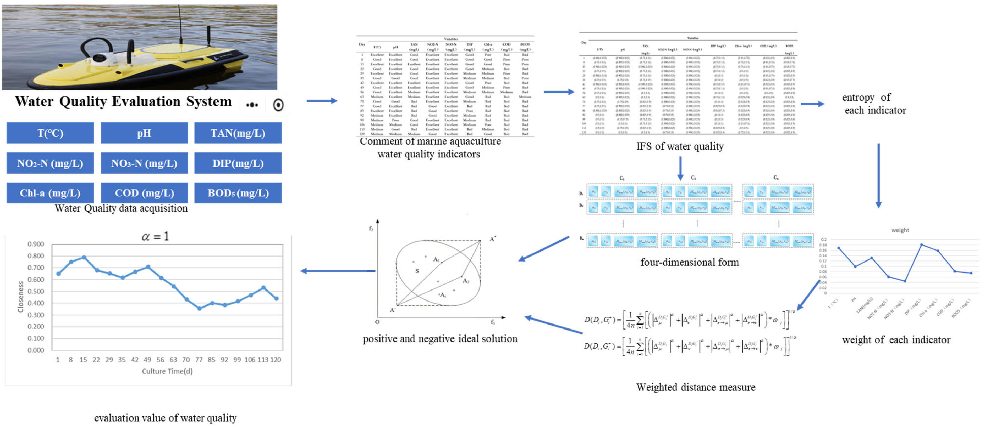
In this section, we will use the same example shown by Ma [33] to apply the evaluation model proposed in this study. The overall methodology of marine culture water quality evaluation is shown in Figure 1.

6.1. Obtain IFS of Marine Aquaculture Water Quality

In this section, we will use the same example shown by Ma [33] to apply the evaluation model proposed in this study. Ma used a modified water quality indicator to evaluate the marine water quality of intensive culture. Similarly, we can apply our improved method to solve the evaluation problem. Nine indicators, namely, TAN, NO₂-N, NO₃-N, DIP, Chl-a, COD, BOD5, pH, and T, were chosen for the evaluation. The basic statistics of water quality are summarized in

Table 5. Mean of water quality indicators determined weekly from 1 July to 28 October 2008, in the marine culture system.

Day	Variables
	T (°C)	pH	TAN (mg/L)	NO2-N (mg/L)	NO3-N (mg/L)	DIP (mg/L)	Chl-a (mg/L)	COD (mg/L)	BOD5 (mg/L)
1	28.6575	8.3	0.0342	0.0022	0.0301	0.1473	0.1088	5.02	4.425
8	26.7225	7.905	0.0473	0.0783	0.0167	0.2921	0.0181	2.6018	3.325
15	29.3575	8.0225	0.0172	0.0037	0.0157	0.1024	0.0233	3.451	3.3
22	30.285	7.7625	0.0424	0.0008	0.014	0.1558	0.0334	6.958	6.35
29	27.5675	7.73	0.0583	0.0234	0.0521	0.3391	0.0337	2.3873	6.725
35	30.8625	7.6625	0.0251	0.034	0.0186	0.2042	0.0264	8.7415	3.725
42	28.8625	7.8725	0.0068	0.0018	0.0361	0.1429	0.1293	8	4.575
49	32.17	7.7525	0.0145	0.0028	0.0239	0.0999	0.0307	2.3965	5.2
56	25.6025	7.9275	0.0721	0.0143	0.0213	0.2419	0.035	1.557	6.925
63	24.9475	8.0525	0.1032	0.1646	0.1403	0.186	0.1622	5.897	2.75
70	27.6925	7.6125	0.8301	0.0295	0.0714	0.2825	0.1861	4.948	5.475
77	25.3475	7.7075	0.4408	0.5185	0.457	1.2834	0.1948	6.1235	5.825
85	29.325	7.8275	0.9874	0.541	0.238	0.8596	0.3234	4.7098	7.925
92	21.6175	7.8125	0.2025	0.4387	0.1365	0.2016	0.1704	8.8915	8.15
99	20.6575	7.14	0.0341	0.3695	0.3227	0.4645	0.2149	16.037	11.9
106	21.6975	7.3175	0.0448	0.3442	0.5815	0.3978	0.1049	12.9953	13.25
113	24.445	7.5225	0.3137	0.3724	0.0201	1.7985	0.0966	8.1792	7.7
120	22.8175	7.3475	0.0671	0.3836	0.2932	1.7985	0.023	12.3805	12.9375

. Ma proposed five interval classes for each indicator. The limits among classes were determined considering the natural variation of these properties in marine culture systems and previous ecological data obtained from experiments about optimal marine culture conditions. The classifications attributed to the classes ranged from I to V, which reflects gradients of suitability for marine culture. These indicators are considered in terms of the development of marine culture and they should also be maintained within appropriate limits in the culture ponds. The five interval classes of the selected water quality variables can be given as shown in

Table 6. The five interval classes (I, II, III, IV, and V) in the selected marine culture water quality indicators.

	Limits of Shrimp Water QUALITY Classes
	I Excellent	II Good	III Medium	IV Poor	V Bad
TAN (mg/L)	<0.02	0.02–0.065	0.065–0.11	0.11–0.155	0.155–0.2
NO2-N (mg/L)	<0.38	0.38–1.38	1.38–2.38	2.38–3.38	3.38–4.38
NO3-N (mg/L)	<1	1–2	2–3	3–4	4–5
DIP (mg/L)	<0.05	0.05–0.2	0.2–0.5	0.5–1	1–1.5
Chl-a (mg/L)	<0.01	0.01–0.026	0.026–0.064	0.064–0.16	0.16–0.4
COD (mg/L)	<0.5	0.5–1	1–2	2–4	4–8
BOD5 (mg/L)	<1	1–2	2–3	3–4	4–5
pH	7.7–8.3	7.5–7.69 or 8.29–8.5	7.3–7.49 or 8.51–8.7	7–7.29 or >8.7	<7 or >8.7
T (°C)	27–30	25–26.9 or 30.1–33	20–24.9 or 33.1–36	18–19.9	<18 or >36

. On the basis of Ma’s research, we construct the comment set, shown in

Table 7. Comments with respect to marine aquaculture water quality indicators determined weekly.

Day	Variables
	T (°C)	pH	TAN (mg/L)	NO2-N (mg/L)	NO3-N (mg/L)	DIP (mg/L)	Chl-a (mg/L)	COD (mg/L)	BOD5 (mg/L)
1	Excellent	Excellent	Good	Excellent	Excellent	Good	Poor	Bad	Bad
8	Good	Excellent	Good	Excellent	Excellent	Good	Good	Poor	Poor
15	Excellent	Excellent	Excellent	Excellent	Excellent	Good	Good	Poor	Poor
22	Good	Excellent	Good	Excellent	Excellent	Good	Medium	Bad	Bad
29	Excellent	Excellent	Good	Excellent	Excellent	Medium	Medium	Poor	Bad
35	Good	Good	Good	Excellent	Excellent	Medium	Medium	Bad	Poor
42	Excellent	Excellent	Excellent	Excellent	Excellent	Good	Poor	Bad	Bad
49	Good	Excellent	Excellent	Excellent	Excellent	Good	Medium	Poor	Bad
56	Good	Excellent	Medium	Excellent	Excellent	Medium	Medium	Medium	Bad
63	Medium	Excellent	Medium	Excellent	Excellent	Good	Bad	Bad	Medium
70	Good	Good	Bad	Excellent	Excellent	Medium	Bad	Bad	Bad
77	Good	Excellent	Bad	Good	Excellent	Bad	Bad	Bad	Bad
85	Excellent	Excellent	Bad	Good	Excellent	Poor	Bad	Bad	Bad
92	Medium	Excellent	Bad	Good	Excellent	Medium	Bad	Bad	Bad
99	Medium	Poor	Good	Excellent	Excellent	Medium	Bad	Bad	Bad
106	Medium	Medium	Good	Excellent	Excellent	Medium	Poor	Bad	Bad
113	Medium	Good	Bad	Excellent	Excellent	Bad	Medium	Bad	Bad
120	Medium	Medium	Medium	Good	Excellent	Bad	Good	Bad	Bad

. There are eighteen days’ worth of marine aquaculture water quality indicators, with each represented by the IFS $D=\{D_1,D_2,\dots ,D_{18}\}$ in the nine indicator spaces $C=\{C_1,C_2,\dots ,C_9\}$.

We convert the comment set into a corresponding IFS according to certain rules and indicator characteristics, shown in

Table 8. Level conversion table of language indicators.

Comment	Intuitionistic Fuzzy Number
Excellent	(0.900, 0.025)
Good	(0.750, 0.150)
Medium	(0.500, 0.500)
Poor	(0.150, 0.750)
Bad	(0.025, 0.900)

. The indicators of water quality $C=\{C_1,C_2,\dots ,C_m\}$ belong to benefit indicators. So, the attribute of indicators in Table 5 is that the higher the indicator is, the better the water quality will be. Based on Property 4 in Definition 3, we give the results in Table 8. Then we can obtain an intuitive fuzzy matrix $X={(({\mu }_{ij},{\nu }_{ij}))}_{18\times 9}$ for evaluating marine aquaculture water quality. The IFSs of marine aquaculture water quality are shown in Appendix C.

6.2. Establishing Positive and Negative Ideal Solutions

All the water quality indicators belong to benefit indicators. So, for each indicator, we establish positive and negative ideal solutions according to Equations (49) and (50). The results are shown in

Table 9. Positive and negative ideal solutions with respect to marine aquaculture water quality indicators.

Indicators	Negative Ideal Solution ${\mathit{G}}_{\mathit{i}}^{+}$	Positive Ideal Solution ${\mathit{G}}_{\mathit{i}}^{-}$
T (°C)	(1, 0)	(0, 1)
pH	(1, 0)	(0, 1)
TAN (mg/L)	(1, 0)	(0, 1)
NO2-N (mg/L)	(1, 0)	(0, 1)
NO3-N (mg/L)	(1, 0)	(0, 1)
DIP (mg/L)	(1, 0)	(0, 1)
Chl-a (mg/L)	(1, 0)	(0, 1)
COD (mg/L)	(1, 0)	(0, 1)
BOD5 (mg/L)	(1, 0)	(0, 1)

.

6.3. Calculating the Weight and Allocation of Each Intuitionistic Fuzzy Number

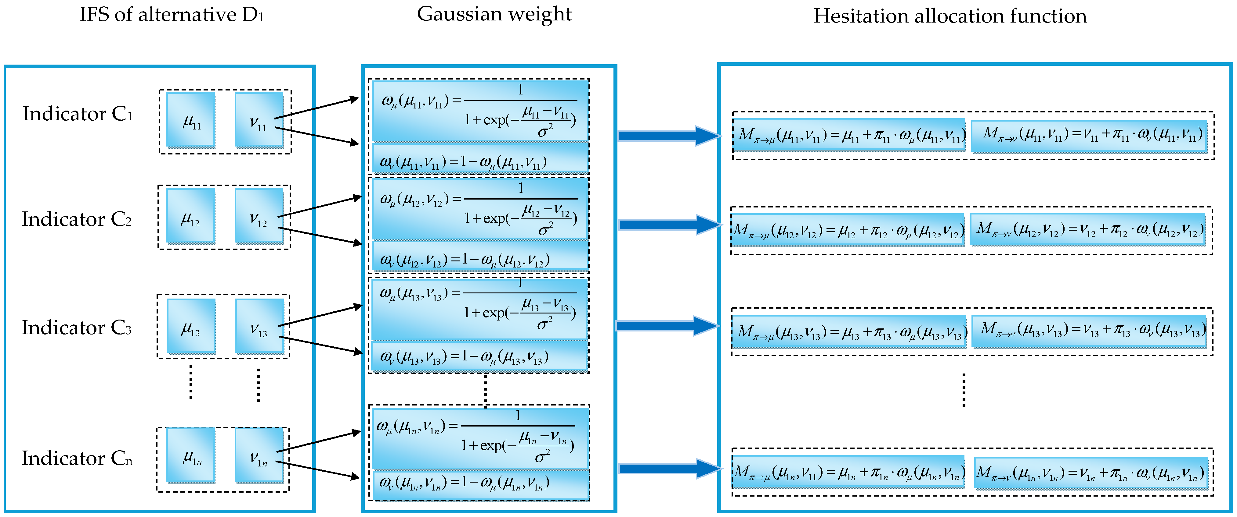
For the intuitionistic fuzzy number of $X={(({\mu }_{ij},{\nu }_{ij}))}_{18\times 9}$, according to Equations (37) and (38), we can calculate the weight of each intuitionistic fuzzy number ${\omega }_{\mu }(x_{ij}),{\omega }_{\nu }(x_{ij})$. The allocation function of membership and non-membership to hesitation $M_{\pi \to \mu },M_{\pi \to \nu }$ can be calculated according to Equations (43) and (44), and we can get the four-dimensional form of each intuitionistic fuzzy number. The process is shown in Figure 2.

6.4. Objective Variable Weight Determination

Based on Equation (48), the weight is shown in

Table 10. Weight of aquaculture water quality variables.

Indicators	T (°C)	pH	TAN (mg/L)	NO2-N (mg/L)	NO3-N (mg/L)	DIP (mg/L)	Chl-a (mg/L)	COD (mg/L)	BOD5 (mg/L)
Weight	0.168	0.099	0.131	0.061	0.045	0.181	0.158	0.081	0.075

. NO₃-N has the lowest weight and DIP has the highest weight. The ranking of weights is DIP > T > Chl-a > TAN > PH > COD > BOD₅ > NO₂-N > NO₃-N.

6.5. Calculating the Weighted Distance Measure of Each Alternative $D_i$ in Terms of Both Positive Ideal Solution $G_i^{+}$ and Negative Ideal Solution $G_i^{-}$

According to Equations (51) and (52), we get the weighted improved distance of each alternative to the positive ideal solution and negative ideal solution, respectively. The results are shown in

Table 11. Weighted distance measure of each alternative in terms of both the positive ideal solution and the negative ideal solution.

Day	Distance
	$\mathit{\alpha }=1$ $\mathbf{D}({\mathbf{D}}_{\mathbf{i}},{\mathbf{G}}_{\mathbf{i}}^{+})$$\mathbf{D}({\mathbf{D}}_{\mathbf{i}},{\mathbf{G}}_{\mathbf{i}}^{-})$		$\mathbf{\alpha }=2$ $\mathbf{D}({\mathbf{D}}_{\mathbf{i}},{\mathbf{G}}_{\mathbf{i}}^{+})$$\mathbf{D}({\mathbf{D}}_{\mathbf{i}},{\mathbf{G}}_{\mathbf{i}}^{-})$		$\mathbf{\alpha }=6$ $\mathbf{D}({\mathbf{D}}_{\mathbf{i}},{\mathbf{G}}_{\mathbf{i}}^{+})$$\mathbf{D}({\mathbf{D}}_{\mathbf{i}},{\mathbf{G}}_{\mathbf{i}}^{-})$
1	0.039	0.072	0.021	0.035	0.067	0.092
8	0.028	0.083	0.012	0.038	0.034	0.089
15	0.023	0.088	0.011	0.040	0.033	0.095
22	0.036	0.075	0.016	0.035	0.044	0.086
29	0.039	0.073	0.019	0.033	0.051	0.085
35	0.043	0.069	0.020	0.030	0.051	0.075
42	0.037	0.074	0.020	0.036	0.067	0.092
49	0.033	0.079	0.015	0.036	0.043	0.087
56	0.043	0.068	0.020	0.029	0.051	0.074
63	0.051	0.060	0.026	0.028	0.078	0.079
70	0.063	0.048	0.030	0.025	0.081	0.073
77	0.072	0.039	0.037	0.022	0.097	0.073
85	0.067	0.045	0.034	0.025	0.089	0.083
92	0.069	0.043	0.032	0.021	0.081	0.055
99	0.065	0.046	0.030	0.022	0.079	0.059
106	0.059	0.052	0.027	0.023	0.069	0.059
113	0.052	0.059	0.024	0.031	0.064	0.091
120	0.062	0.049	0.031	0.023	0.091	0.068

with $\alpha =1,2,6$. In the distance definition mentioned in Section 3, $\alpha =1$ represents the Hamming distance, $\alpha =2$ represents the Euclidean distance, and $\alpha =6$ represents the higher-order distance. In their application to marine aquaculture water quality, they correspond to different evaluation strategies:

• $\alpha =1$: Treat all deviations in water quality indicators equally. They are applicable to situations where a comprehensive assessment of overall water quality deviation is required. Even if each indicator is off by just a little, the cumulative effect can still reveal issues.
• $\alpha =2$: While comprehensively considering all indicators, naturally give more attention to those with significant deviations. This balances the overall consistency and sensitivity to key deviations, and it is the most common choice in practice.
• $\alpha =6$: Only focus on the metric with the largest deviation. This has strong practical significance in water quality safety, meaning that even if only one indicator is seriously out of limits (for example, NO₃-N suddenly spikes), it may cause the widespread death of fish and shrimp. This corresponds to the idea that “the weakest link determines the safety”.

6.6. Calculating the Closeness of Each Alternative $M(D_i)$

According to Equation (53), we get the closeness of each alternative $M(D_i)$, shown in

Table 12. Closeness of each alternative.

Day	Closeness
	$\mathit{\alpha }=1$	$\mathit{\alpha }=2$	$\mathit{\alpha }=6$
1	0.650	0.631	0.577
8	0.751	0.765	0.726
15	0.790	0.792	0.739
22	0.679	0.687	0.661
29	0.653	0.630	0.625
35	0.617	0.605	0.595
42	0.667	0.638	0.579
49	0.707	0.701	0.670
56	0.614	0.589	0.591
63	0.544	0.518	0.505
70	0.432	0.455	0.474
77	0.355	0.377	0.429
85	0.401	0.423	0.483
92	0.383	0.392	0.401
99	0.415	0.431	0.428
106	0.468	0.463	0.460
113	0.532	0.563	0.585
120	0.438	0.434	0.428

. As the indicators belong to benefit indicators, the bigger $M(D_i)$ is, the better the water quality of alternative $D_i$ will be.

The closeness distributed into five classes (I, II, III, IV, V) indicating the suitability of marine aquaculture water quality is shown in

Table 13. The closeness distributed into five classes (I, II, III, IV, V) indicating the suitability of the marine aquaculture water quality.

Water Condition	Evaluation Classes	$\mathit{\alpha }=1$	$\mathit{\alpha }=2$	$\mathit{\alpha }=6$
Excellent	I	0.680–0.790	0.702–0.792	0.671–0.739
Good	II	0.545–0.679	0.606–0.701	0.576–0.670
Medium	III	0.469–0.544	0.464–0.605	0.506–0.575
Poor	IV	0.402–0.468	0.393–0.463	0.430–0.505
Bad	V	0.355–0.401	0.377–0.392	0.401–0.429

. Figure 3 is the water quality closeness of each alternative within the whole culture period. Although the value of water quality closeness varies, the trend is consistent. The early stage of culture time is rated as excellent or good. When $\alpha$ is 1, the water quality closeness value for the first 56 days of aquaculture is between 0.741–0.626. When $\alpha$ is 2, the water quality closeness value for the first 56 days of aquaculture is between 0.662–0.583. When $\alpha$ is 6, the water quality closeness value for the first 56 days of aquaculture is between 0.566–0.529. After 63 days, the water quality closeness begins to decline, with a rating of medium to bad. When $\alpha$ is 1, the water quality closeness value for the latter 60 days of aquaculture is between 0.589–0.432. When $\alpha$ is 2, the water quality closeness value for the latter 60 days of aquaculture is between 0.56–0.46. When $\alpha$ is 6, the water quality closeness value for the latter 60 days of aquaculture is between 0.524–0.482. The results indicate that water management should be intensified in the later culture period. The result coincides with that of Ma’s [33]. However, Ma used the water quality index for marine aquaculture water quality evaluation, which is a complex process that needs voluminous calculations. The method proposed in this study reduces computational complexity and is easy to apply in many fields.

7. Discussion and Conclusions

Based on the comparison of distance measures for IFSs in Section 4, we can get that the improved distance measure proposed in this study can overcome the drawbacks of existing distance measures. It is an effective and rational method for IFS distance measuring, with improved accuracy. Based on its application to marine aquaculture water quality evaluation in Section 6, the results demonstrate that the improved IFS TOPSIS based on the proposed distance measure has the following advantages: (1) The data process is relatively simple and keeps the original information; (2) evaluation output data is understandable and acceptable; (3) the method has a wide range of applications, such as pattern recognition, image processing, and medical diagnosis. For further research, it will be necessary to consider the construction of hesitant fuzzy sets to address more complex situations and to improve the evaluation model.

The marine aquaculture environment is complex and ever-changing, with various types of water quality indicators. Therefore, the rapid quantitative evaluation of aquaculture water has always been considered a complex decision-making process. So, this study applies IFSs to describe the uncertainty and ambiguity of marine aquaculture water evaluation indicators.

Based on a detailed analysis of existing distance measures for IFSs, this study proposes a new distance measure that not only considers membership and non-membership information, but also constructs an allocation function for membership and non-membership, introducing hesitation information into distance metrics. We proposed the definitions and proved their properties. The results indicate that IFSs can describe the fuzzy characteristics of expert comments, and the improved distance measure solves the problem of introducing hesitation allocations. Weekly marine water quality tests from 1 July to 28 October 2008 are used as examples. TAN, NO₂-N, NO₃-N, DIP, Chl-a, COD, BOD5, pH, and T are chosen as water quality indicators. The ranking of weights is DIP > T > Chl-a > TAN > PH > COD > BOD5 > NO₂-N > NO₃-N. Although the value of water quality closeness varies, the trend is consistent. In the first 56 days of aquaculture, the level of water quality is excellent or good. Over the latter 60 days, the water quality closeness begins to decline. The level of water quality moves from medium to bad. Both the theoretical analysis and practical application demonstrate that the proposed distance measure can overcome the drawbacks of existing distance measures and get rational results.

In this study, the IFS TOPSIS method based on the proposed distance measure has been proposed and verified with respect to marine aquaculture water quality evaluation. The results demonstrate that the proposed method in this study reduces computational complexity and can be easily applied to many fields. Of course, there are some limitations in this study. Specifically, when faced with more complex decision-making processes, such as in group decision-making, the proposed method is not applicable. Moreover, there is a lack of consideration for hesitation data in the research process. In practical evaluations, experts may have limited understanding of the evaluated object due to their own professional knowledge and may not be able to provide definitive comments on all indicators. This can manifest as hesitation in criticizing a certain event or object, or even as multiple different evaluation values for indicators. In further research, it is necessary to consider constructing hesitant fuzzy sets to solve more complex situations and improve the evaluation model.

References

1. Xin, N.; Zhang, S.; Yang, Y.; Xin, K. Analysis on development process and current situation of Tianjin industrial marine aquaculture. Fish. Mod. 2019, 46, 1–6. [Google Scholar]
2. Wang, Y.; Huang, T.; Tian, X.; Chen, W.; Xiao, M. Optimized Design and Energy Consumption Analysis of an Improved Feeding Equipment Structure Based on Numerical Simulation. J. Comput. Methods Sci. Eng. 2024, 24, 3531–3544. [Google Scholar] [CrossRef]
3. Cao, L.; Wang, W.; Yang, Y. Environmental impact of aquaculture and countermeasures to aquaculture pollution in China. Environ. Sci. Pollut. Res.–Int 2007, 14, 452–462. [Google Scholar] [PubMed]
4. Martinaiou, P.; Manoli, P.; Boti, V.; Hela, D.; Makou, E.; Albanis, T.; Konstantinou, I. Quality Control of Emerging Contaminants in Marine Aquaculture Systems by Spot Sampling-Optimized Solid Phase Extraction and Passive Sampling. Sustainability 2022, 14, 3452. [Google Scholar] [CrossRef]
5. Kan, W.; Fan, D.; Zhang, Q.; Tu, J. Seasonal Variation and Assessment of Water Quality in Bohai in Tianjin Shore Sea Areas. Trans. Oceanol. Limnol. 2016, 1, 25–29. [Google Scholar]
6. Wang, Y.; Zhang, Y.; Ma, F.; Tian, X.; Ge, S.; Man, C.; Xiao, M. Research on Precise Feeding Strategies for Large-Scale Marine Aquafarms. J. Mar. Sci. Eng. 2024, 12, 1671. [Google Scholar] [CrossRef]
7. Xu, Y.; Wei, X.; Li, J.; Wu, X.; Ma, Y.; Sun, W. Characteristics of Environment Parameters and Eutrophication Assessment of Seawater in Laizhou Bay in Spring and Summer, 2013. Environ. Monit. China 2016, 32, 63–69. [Google Scholar] [CrossRef]
8. Ferreira, N.C.; Bonett, C.; Seiffert, W.Q. Hydrological and water quality indices as management tools in marine shrimp culture. Aquaculture 2011, 318, 425–433. [Google Scholar] [CrossRef]
9. Zhang, X.; Zhang, Y.; Zhang, Q. Evaluation and Analysis of Water Quality of Marine Aquaculture Area. Int. J. Environ. Res. Public Health 2020, 17, 1446. [Google Scholar] [CrossRef]
10. Zhao, E.; Kuo, Y.; Chen, N. Assessment of water quality under various environmental features using a site-specific weighting water quality index. Sci. Total Environ. 2021, 783, 146868. [Google Scholar] [CrossRef]
11. Nong, X.; Shao, D.; Zhong, H.; Liang, J. Evaluation of water quality in the South-to-North Water Diversion Project of China using the water quality index (WQI) method. Water Res. 2020, 178, 115781. [Google Scholar] [CrossRef]
12. Zadeh, L.A. Fuzzy sets. Inf. Control. 1965, 8, 338–353. [Google Scholar] [CrossRef]
13. Yang, Y.; Li, B.; Li, C.; Liu, P.; Li, T.; Luo, Y.; Yang, L.; Che, L.; Li, M. Spatiotemporal comprehensive evaluation of water quality based on enhanced variable fuzzy set theory: A case study of a landfill in karst area. J. Clean. Prod. 2024, 450, 141882. [Google Scholar] [CrossRef]
14. Fang, Y.; Zheng, X.; Peng, H.; Wang, H.; Xin, J. A new method of the relative membership degree calculation in variable fuzzy sets for water quality assessment. Ecol. Indic. 2019, 98, 515–522. [Google Scholar]
15. Liang, G.; Jia, Z.; Gao, Y. Water quality evaluation of the mainstream of Liaohe River based on fuzzy membership model. J. Environ. Eng. Technol. 2021, 11, 693–700. [Google Scholar]
16. You, G.; Xu, B.; Su, H.; Zhang, S.; Pan, J.; Hou, X.; Li, J.; Ding, R. Evaluation of Aquaculture Water Quality Based on Improved Fuzzy Comprehensive Evaluation Method. Water 2021, 13, 1019. [Google Scholar] [CrossRef]
17. Atanassov, K.; Stoeva, S. Intuitionistic fuzzy sets. Fuzzy Sets Syst. 1986, 31, 343–349. [Google Scholar]
18. Atanassov, K. Intuitionistic Fuzzy Sets: Theory and Applications; Springer: Berlin/Heidelberg, Germany, 1999; pp. 15–26. [Google Scholar]
19. Bustince, H.; Burillo, P. Correlation of interval-valued intuitionistic fuzzy sets. Fuzzy Sets Syst. 1995, 74, 237–244. [Google Scholar] [CrossRef]
20. Wang, W.; Xin, X. Distance measure between intuitionistic fuzzy sets. Pattern Recognit. Lett. 2005, 13, 2063–2069. [Google Scholar] [CrossRef]
21. Szmidt, E.; Kasprzyk, J. Distances between intuitionistic fuzzy sets. Fuzzy Sets Syst. 2000, 114, 505–518. [Google Scholar] [CrossRef]
22. Xu, Z. Some similarity measures of intuitionistic fuzzy sets and their applications to multiple attribute decision making. Fuzzy Optim. Decis. Mak. 2007, 6, 109–121. [Google Scholar] [CrossRef]
23. Liu, H. New similarity measures between intuitionistic fuzzy sets and between elements. Math. Comput. Model. 2005, 42, 61–70. [Google Scholar] [CrossRef]
24. Grzegorzewski, P. Distances between intuitionistic fuzzy sets and/or interval-valued fuzzy sets based on the Hausdorff metric. Fuzzy Sets Syst. 2004, 148, 319–328. [Google Scholar] [CrossRef]
25. Hung, W.; Yang, M. Similarity measures of intuitionistic fuzzy sets based on Hausdorff distance. Pattern Recognit. Lett. 2004, 25, 1603–1611. [Google Scholar] [CrossRef]
26. Yang, Y.; Chiclana, F. Consistency of 2D and 3D distances of intuitionistic fuzzy sets. Expert Syst. Appl. 2012, 39, 8665–8670. [Google Scholar] [CrossRef]
27. Chen, S.; Cheng, S.; Lan, T. A novel similarity measure between intuitionistic fuzzy sets based on the centroid points of transformed fuzzy numbers with applications to pattern recognition. Inf. Sci. 2016, 343, 15–40. [Google Scholar] [CrossRef]
28. Shen, F.; Ma, X.; Li, Z. An extended intuitionistic fuzzy TOPSIS method based on a new distance measure with an application to credit risk evaluation. Inf. Sci. 2017, 428, 105–119. [Google Scholar] [CrossRef]
29. Li, X.; Suo, C.; Li, Y. Width-based distance measures on interval-valued intuitionistic fuzzy sets. J. Intell. Fuzzy Syst. 2021, 40, 8857–8869. [Google Scholar] [CrossRef]
30. Hwang, C.; Yoon, K. Multiple Attribute Decision Making; Springer: Berlin/Heidelberg, Germany, 1981; pp. 15–19. [Google Scholar]
31. Joshi, D.; Kumar, S. Intuitionistic fuzzy entropy and distance measure based TOPSIS method for multi-criteria decision making. Egypt. Inform. J. 2014, 15, 97–104. [Google Scholar] [CrossRef]
32. Chen, Z.; Yang, W. A new multiple criteria decision-making method based on intuitionistic fuzzy information. Expert Syst. Appl. 2012, 39, 4328–4334. [Google Scholar] [CrossRef]
33. Ma, Z.; Song, X.; Wan, R.; Lei, G. A modified water quality index for intensive shrimp ponds of Litopenaeus vannamei. Ecol. Indic. 2013, 24, 287–293. [Google Scholar] [CrossRef]
Figure 1. Overall methodology of marine culture water quality evaluation.
Water 18 00712 g001
Figure 2. Process of weight and allocation function calculation for each intuitionistic fuzzy number.
Water 18 00712 g002
Figure 3. The closeness of each alternative within the whole culture period, generated over 120 days (from 1 July to 28 October 2008). Data are expressed as the closeness of water quality versus the number of culture days with α = 1 , 2 , 6 , respectively.
Water 18 00712 g003