Comparison of Improved Fisher Discriminant Analysis and Random Forest for Mine Water Inrush Source Identification: Performance in Single-Mine and Multi-Mine Scenarios

Abstract

Rapid and accurate identification of water inrush sources is essential for the prevention and control of coal mine water hazards. Fisher discriminant analysis and random forest are widely applied, but their performance comparison and applicability under single-mine and multi-mine scenarios remain to be investigated. This study takes the Tunlan Mine in Shanxi Province, China, as an example and evaluates both models using accuracy, precision, recall, F1-score, and confusion matrix. A joint discrimination scheme is used to explore their generalization ability. In the single-mine scenario, the improved Fisher algorithm achieves an overall accuracy of 93% and the random forest model achieves 87%, indicating that the former has greater advantages when data distribution is relatively linear. In the multi-mine joint discrimination scenario, the random forest model yields accuracies of 77–98%, far exceeding those of the Fisher algorithm and demonstrating clear superiority in handling complex nonlinear data. The results show that model performance depends primarily on data quality and feature distribution rather than solely on sample size. This study provides a scientific basis for selecting water source identification algorithms in different scenarios and has practical value for improving coal mine water hazard prevention and control.

1. Introduction

China has a massive scale of coal resource extraction, but mine water inrush accidents associated with mining pose a major threat to coal mine safety and production due to their sudden onset and severe destructiveness [1,2,3]. Mine water inrush accidents often occur abruptly with substantial damage, posing a significant threat to the lives of underground personnel and presenting enormous challenges for emergency response and disaster management. Any effective measure for mine water hazard prevention and control has as its primary prerequisite the rapid and accurate identification of water inrush sources [4]. Traditional methods largely rely on expert experience and simplified hydrogeochemical analysis; however, when confronted with similar chemical characteristics or mixed water sources from multiple aquifers, discrimination is often ambiguous, readily leading to delays in prevention and control measures [5].

Traditional methods typically depend on expert experience and hydrogeochemical analysis, and they struggle to provide unequivocal conclusions when dealing with similar chemical characteristics or mixed water sources originating from multiple aquifers. To overcome the limitations of traditional methods, researchers have developed a series of quantitative discrimination models based on hydrochemical data, with iterative advancements manifesting as the expansion and integration from classical statistical methods to modern machine learning and deep learning approaches [6].

First, classical statistical methods represented by Fisher discriminant analysis and their optimizations are characterized by model transparency and strong interpretability, serving as the cornerstone of mine water source identification. Early studies focused on enhancing the performance of traditional mathematical models are as follows: Wu et al. [7] integrated groundwater dynamic response, geothermal gradient calculation, and a combination of Piper diagram-Fisher discriminant analysis-chloride mass balance to achieve quantitative evaluation of multi-source mixed water. Bi et al. [8] incorporated fuzzy clustering and factor analysis to reduce seven ion indicators to four independent variables, improving cross-validation discrimination accuracy from 86.5% to 89.2%. Sun et al. [9] employed the centroid distance evaluation method to assist Fisher discriminant analysis, quantitatively increasing discrimination accuracy from 60% to 83.3%. Dong et al. [10] proposed an intelligent water inrush source identification model combining Fisher feature extraction with SVM, achieving a 12.1% accuracy improvement over traditional SVM and confirming strong hydraulic connectivity between two aquifers in the Wuhai mining area.

Other mathematical methods also exhibit distinct characteristics in the discrimination process. For instance, Bayesian discriminant analysis demonstrates high efficiency with small sample sizes and interfering data; Li et al. [11] applied Bayesian methods combined with hydrogen and oxygen stable isotope theory to achieve quantitative calculation of mixed water sources in the Longfeng Coal Mine. Qian et al. [12] employed Bayesian discriminant analysis and geostatistical methods, attaining a Bayesian discrimination accuracy of 86.09% while revealing that aquifer mixing reduces model accuracy. Gray relational analysis [13] and dynamic weight-entropy weight membership models for water inrush source identification [14] have also been successfully applied. However, the performance of these mathematical methods largely depends on the linear separability of the data.

With advances in computational technology, machine learning and deep learning models have gradually become the frontier and mainstream of research due to their powerful nonlinear fitting capabilities. Support vector machines (SVM) represent an early exploration direction; Lu et al. [15] proposed a hybrid model integrating kernel principal component analysis with an improved sparrow search algorithm-optimized SVM, achieving a test set accuracy of 90.48% in the Gubei Coal Mine. In recent years, ensemble learning and deep learning models have shown particularly outstanding performance. As a representative ensemble algorithm, random forest (RF) was introduced by Yang et al. [16] for mine water source discrimination, achieving an identification accuracy of 87% for five water source types in the Pingdingshan mining area and identifying Ca²⁺ as the most important discriminant indicator; Max et al. [17] combined laser-induced fluorescence spectroscopy with RF, reaching 100% identification accuracy for seven mixed samples. Gradient boosting models perform equally well; Wang et al. [18] integrated tree-structured Parzen estimator with LightGBM, attaining a model accuracy of 93.1%; Yang et al. [19] constructed a gradient boosting decision tree model that achieved 95.8% identification accuracy on 24 unknown samples in the Pingdingshan mining area. In the deep learning domain, Jiang et al. [20] first introduced deep feedforward networks to process big data from 1952 water samples, achieving a test accuracy of 96.68% in the Panxie mining area; Cui et al. [21] combined swarm intelligence optimization algorithms with deep feedforward neural networks, yielding a GWO-DFNN model identification accuracy of 95.92%. Additionally, Li et al. [22] pioneered the use of ultraviolet-visible absorption spectroscopy combined with a GA-XGBoost model, achieving an average accuracy of 94% for mixed water source identification; Fang [23] proposed a convolutional neural network-based method that attained a spectral data identification rate of 91.07%. Although these intelligent algorithms exhibit strong performance, their “black-box” nature also poses challenges to interpretability.

To further enhance performance and address specific issues, hybrid models and innovative technical approaches continue to emerge. For example, Wei et al. [24] integrated Fisher discriminant analysis, self-organizing maps, and gray wolf algorithm-optimized SVM (GWOSVM), achieving 100% identification on 20 test samples in the Zhaogezhuang Coal Mine. Zeng et al. [25] innovatively combined groundwater level response, hydrochemistry, random forest, transient electromagnetics, and other techniques to propose a dual verification and quantitative traceability method. Ju et al. [26] developed a dynamic water source identification model incorporating exponential whitening functions and CRITIC-weighted gray situational decision-making, with accuracy exceeding 85%. Li et al. [27] proposed three mixing degree calculation models based on the geometric distribution of mixed water samples, providing new tools for mixed water source analysis.

Among the diverse methods, Fisher discriminant analysis and random forest algorithms represent typical parametric linear models and nonparametric nonlinear ensemble models, respectively, forming a sharp contrast in principles, performance, and interpretability [28,29]. However, existing studies predominantly focus on the application and optimization of individual algorithms or evaluate them solely in single-mine scenarios. Systematic empirical research is still lacking regarding their performance comparison, applicability boundaries, and complementary advantages/disadvantages across different application scenarios, such as single-mine and multi-mine joint discrimination.

Therefore, taking the Tunlan Mine in Shanxi Province as an example, this study aims to systematically compare the effectiveness of improved Fisher discriminant analysis and random forest algorithms in mine water inrush source identification. The research comprehensively employs multiple metrics, including accuracy, precision, recall, F1-score, and confusion matrix, to evaluate the baseline performance of the two models in a single-mine scenario. Furthermore, multi-mine joint discrimination experiments are conducted to investigate their generalization ability and robustness, with the goal of providing a scientific basis for algorithm selection under varying hydrogeological conditions and data scenarios.

2. Materials and Methods

2.1. Study Area

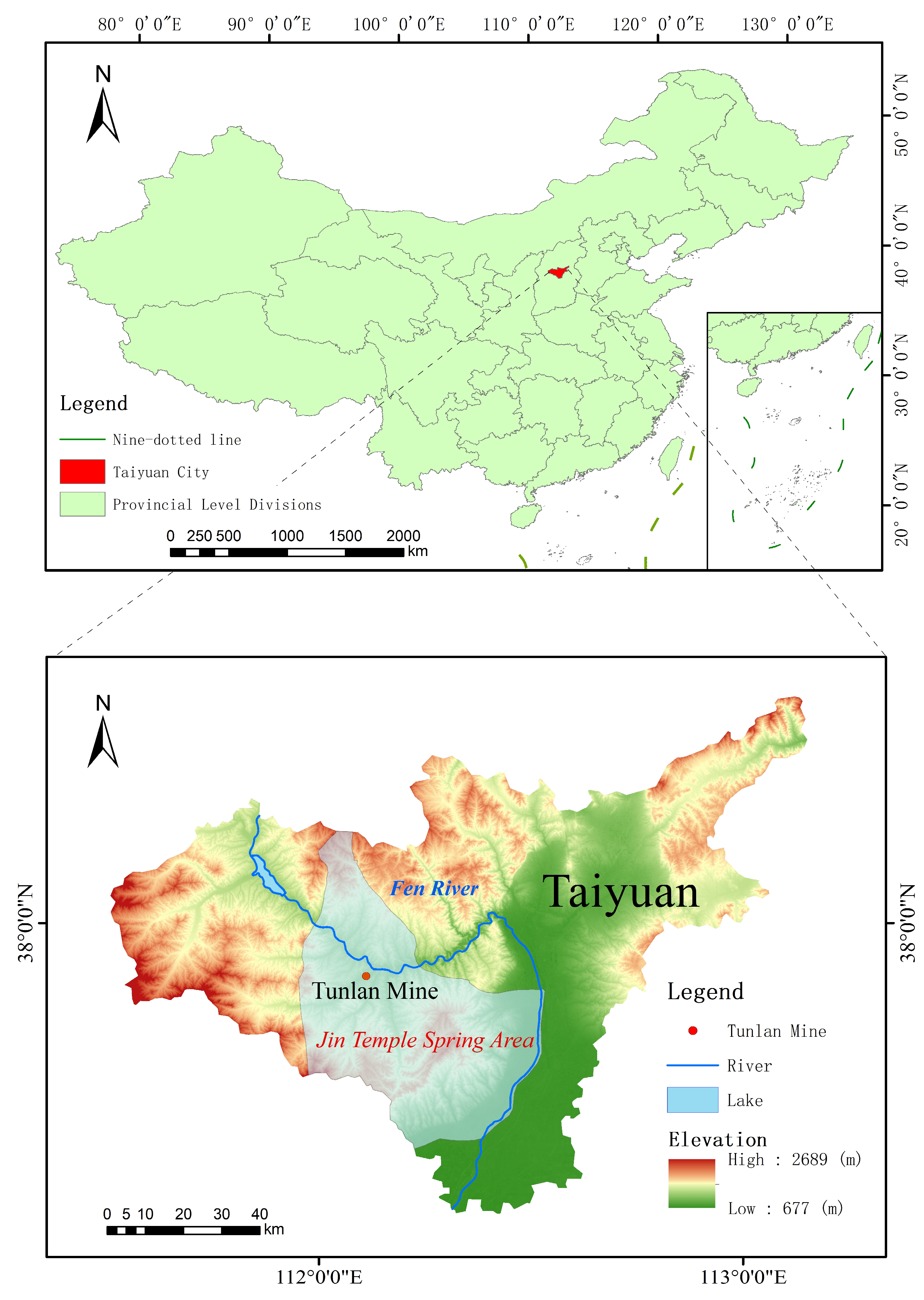
The Tunlan Coal Mine is located in the northwestern part of the Xishan Coalfield in Taiyuan, Shanxi Province, China, on the eastern limb of the Malan Syncline. The topography is generally higher in the southwest and lower in the northeast. The annual average precipitation in the area is approximately 460 mm, primarily concentrated from July to September. Tributaries of the Fen River, including the Tunlan River, Yuanping River, and Dachuan River, flow through the mining field and provide certain recharge to groundwater. The extent of the Jinci Spring domain, within which the Tunlan Mine is located and from which water samples were collected for this study, is outlined. To facilitate understanding of the study area’s location, the following diagram is provided as Figure 1. Figures were prepared using OriginPro 2024 (64-bit) SR1 10.1.0.178, ArcMap 10.8, and CorelDRAW 2024 (v25.0.0.230).

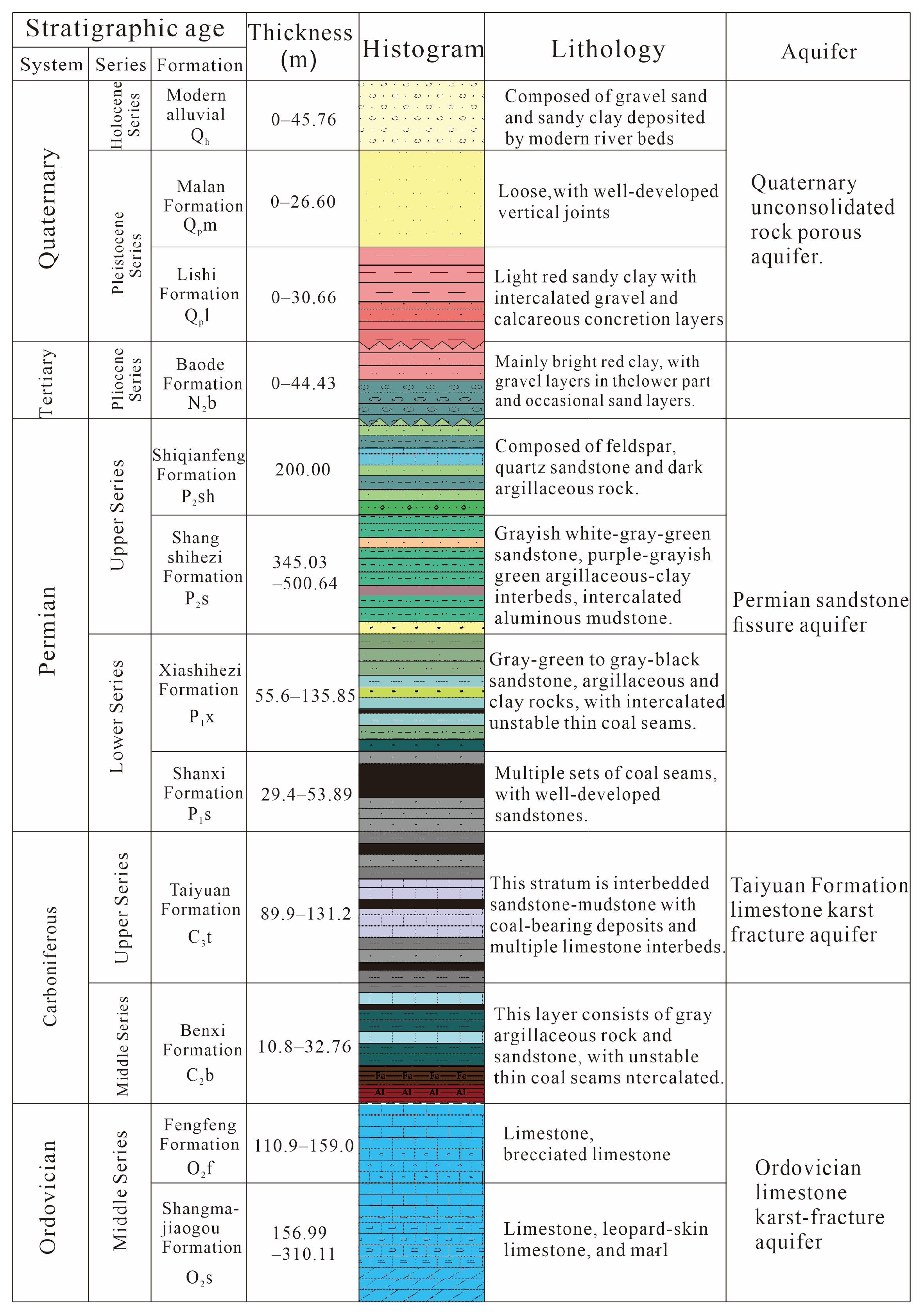
Figure 2 presents the stratigraphic column of the Tunlan Mine area, from the Quaternary at the top to the Middle Ordovician at the base. This succession corresponds to the strata referred to in the text: the Neogene and Quaternary systems; the Upper Permian Upper Shihezi and Shiqianfeng Formations and the Lower Permian Lower Shihezi and Shanxi Formations; the Upper Carboniferous Taiyuan Formation and the Middle Carboniferous Benxi Formation; and the Middle Ordovician Series. The column also indicates the main aquifer and aquitard units: the Quaternary Holocene sand and gravel porous aquifer; the Permian Shihezi and Shanxi Formations sandstone fissure aquifer; the Carboniferous Taiyuan Formation sandstone–limestone fissure aquifer; and the Ordovician limestone karst aquifer. The Benxi Formation (aluminous mudstone, shale, and sandstone) between the coal floor and the top of the Ordovician forms the key aquitard that normally blocks upward flow of Ordovician limestone water; in areas where faults or collapse columns are developed, this barrier may be compromised and form potential water-conducting pathways.

The aquifer system in the mining area mainly comprises the Quaternary Holocene sand and gravel porous aquifer group, the Permian Shihezi and Shanxi Formations sandstone fissure aquifer group, the Carboniferous Taiyuan Formation sandstone interbedded with thin limestone fissure aquifer group, and the Ordovician limestone karst aquifer group. The Quaternary sand and gravel aquifer is distributed in the valleys of the Fen River and its tributaries and exhibits strong permeability, readily receives recharge from precipitation and surface water, and has high water abundance. The sandstone fissure aquifers in the Shihezi and Shanxi Formations generally have weak water abundance. The limestone in the Taiyuan Formation also exhibits poor water yield. The Ordovician karst aquifer group serves as the primary water-filled aquifer for mining of the lower coal group and represents a potential source of floor water inrush, posing a confined pressure threat to lower group coal mining. Goaf water originates from accumulated water in historical goaf areas of the upper and lower coal groups, with complex distribution and variable hydrochemical characteristics. These two sources pose the greatest threat to mine safety and production and are the primary targets for water inrush source identification. The aquitards in the area mainly consist of mudstone, sandstone, and limestone assemblages with good impermeable performance. The Benxi Formation’s aluminous mudstone, shale, and sandstone between the coal floor and the top of the Ordovician system constitute the key aquitard blocking upward flow of Ordovician limestone water. However, in areas where faults, collapse columns, and other structures are developed, the integrity and impermeable performance of these layers may be compromised, potentially forming water-conducting pathways that require particular attention. This study primarily focuses on the Tunlan Mine within the Jinci Spring domain, with data from other mining areas incorporated for model validation and comparison.

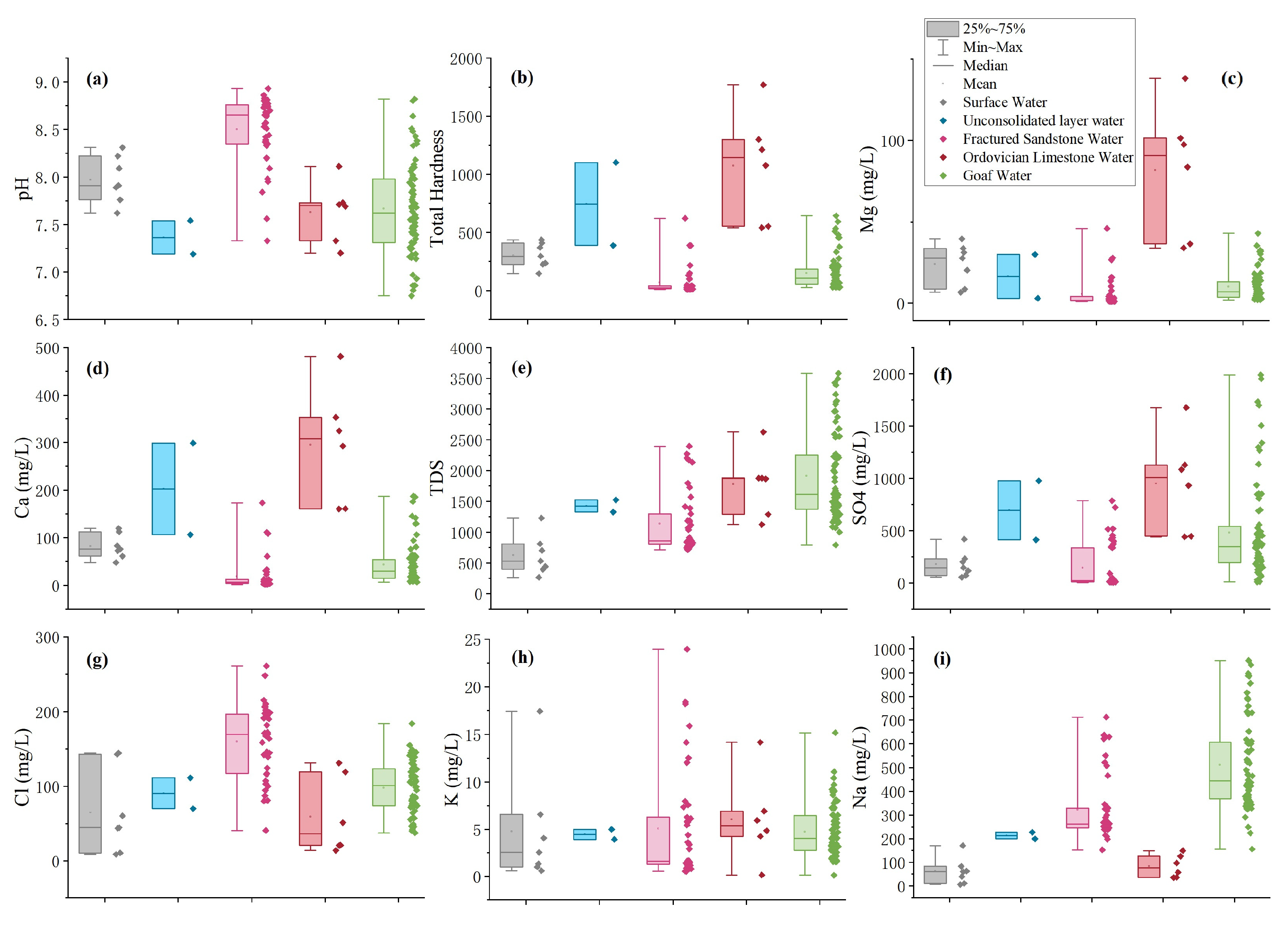
Hydrochemical measurements were obtained using an ion chromatograph (ICS-2100; Thermo Fisher Scientific (China) Co., Ltd., Shanghai, China), a UV–Vis spectrophotometer (UV2800; Shanghai Sunny Hengping Scientific Instrument Co., Ltd., Shanghai, China), and an ICP-MS instrument (iCAP RQ plus; Thermo Fisher Scientific (China) Co., Ltd., Shanghai, China). Prior to analysis, outlier removal was performed in three steps: (1) exclusion of samples marked as anomalous during fieldwork or analysis; (2) removal of samples with values outside plausible physicochemical ranges (e.g., pH, negative concentrations); and (3) exclusion of samples whose cationic–anionic balance error exceeded 5%, computed as |(Σ cations − Σ anions)/(Σ cations + Σ anions)| × 100% in meq/L. The following box plots present statistical analyses of the water sample data after this outlier removal.

In Figure 3, in each small picture from left to right, the water types are surface water, unconsolidated layer water, fractured sandstone water, Ordovician limestone water, and goaf water. Analysis reveals that parameters for surface water and unconsolidated layer water exhibit limited variation and concentrated distributions, distinctly differing from other water samples. In contrast, parameters for fractured sandstone water, Ordovician limestone water, and goaf water generally show broad and scattered distributions, with considerable overlap in certain data (e.g., TDS, K⁺, pH). In particular, the composition of goaf water, influenced by long-term hydrochemical processes, exhibits high overlap with other water samples, often leading to confusion in identification. These data indicate that the Tunlan Mine not only features diverse water quality types but also substantial intra-type variation in ion concentrations with wide coverage ranges, rendering discrimination based solely on hydrochemical data highly challenging. Therefore, appropriate alternative methods are required to develop water source identification models suitable for the aforementioned water sources.

In this study, the classification target is the water source type, i.e., the class label of each water sample. It is encoded as a categorical variable Y with five classes: 0 = surface water, 1 = unconsolidated layer water, 2 = Permian sandstone fissure water, 3 = Ordovician limestone water, and 4 = goaf water. The input features (FEATURES) are the hydrochemical indicators used for discrimination. For the improved Fisher discriminant model, the selected features are total hardness (X₁), pH (X₂), K⁺ (X₃), K⁺% (X₄), Na⁺% (X₅), Cl⁻% (X₆), SO₄²⁻ (X₇), and HCO₃⁻% (X₈). For the random forest model, the feature set additionally includes other measured ions and derived indices (e.g., Na⁺, temporary hardness, TDS). Thus, the discrimination task is to predict the water source label (Y) from the hydrochemical feature vector (X).

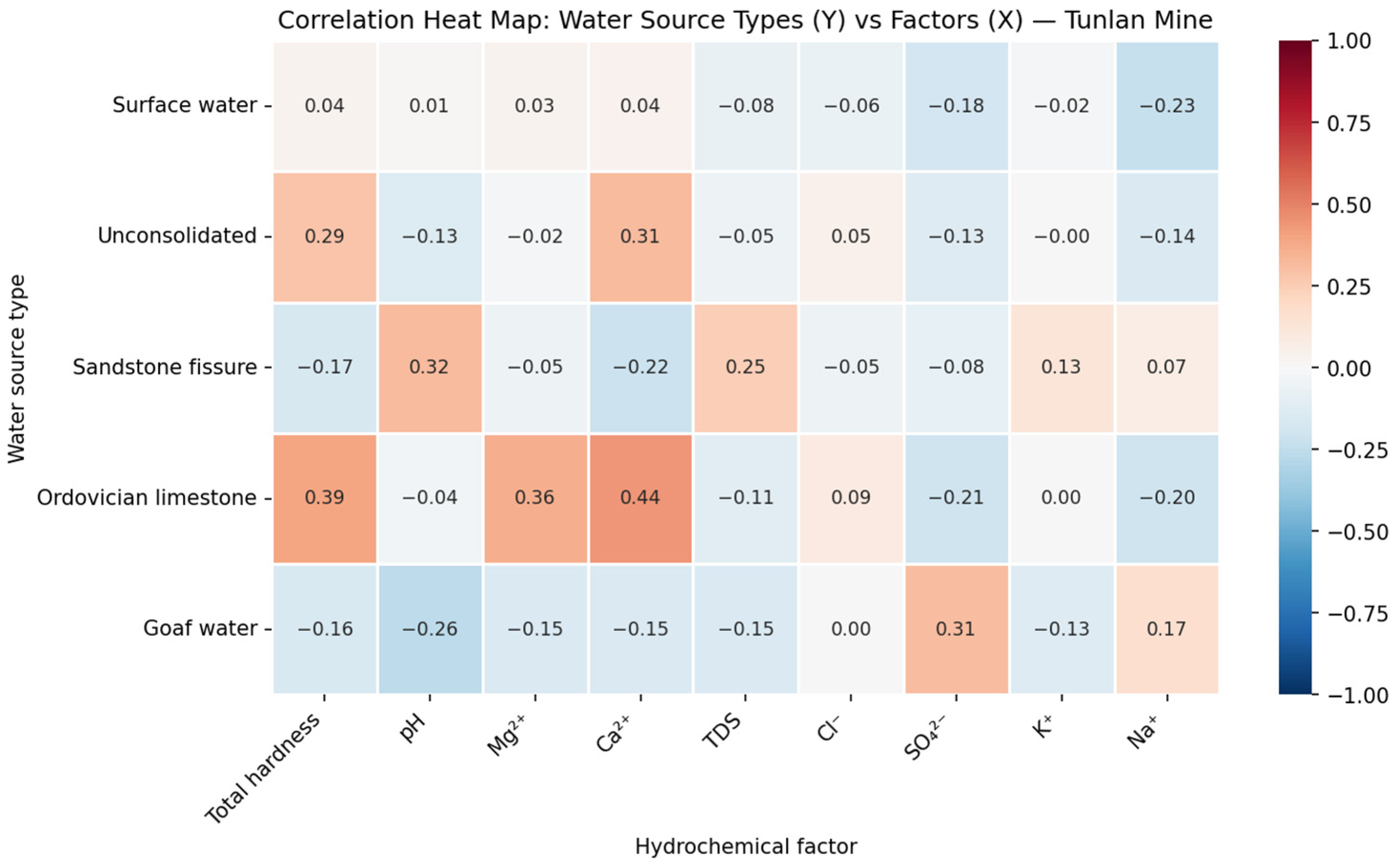
To further illustrate the relationship between the target variable (water source type) and the input features (hydrochemical indicators), a correlation heat map was constructed with the five water source types (surface water, unconsolidated layer water, Permian sandstone fissure water, Ordovician limestone water, and goaf water) on the vertical axis and nine factors (total hardness, pH, Mg, Ca, TDS, Cl, SO₄²⁻, K⁺, and Na⁺) on the horizontal axis (Figure 4).

The correlation coefficients between individual ions or indices and each water source type are generally moderate in magnitude rather than strongly linear. This pattern indicates that the relationship between hydrochemistry and water source identity in the Tunlan Mine is complex: no single factor alone can reliably separate the five types, and discrimination depends on the joint effect of multiple variables and possibly nonlinear combinations. Such complexity underscores the necessity of using multivariate discriminant algorithms—such as the improved Fisher discriminant analysis and random forest applied in this study—rather than relying on one or two hydrochemical indicators for water inrush source identification.

2.2. Model Construction

Models were implemented in Python 3.9.13 within Conda 23.7.4 (Spyder 5.2.2).

2.2.1. Fisher Discriminant Analysis

(1)

Principles of Fisher Discriminant Analysis and Model Improvement

The core principle of the Fisher classification algorithm is linear discriminant analysis (LDA). Its objective is to identify an optimal projection direction that maximizes between-class distance while minimizing within-class distance, thereby achieving dimensionality reduction by projecting the data onto this direction. In the resulting low-dimensional space, the Fisher discriminant function is obtained and compared with the centroid of each class to yield the classification result [16].

Suppose there are c classes in total, with corresponding sample sets denoted as X₁, X₂, …, X_c. The sample set of the i-th class is

$$X_i=\left.\left\{x_1^{\left(i\right)},x_2^{\left(i\right)},\dots ,x_{n_i}^{\left(i\right)}\right.\right\}$$

(1)

where (i) denotes the i-th class, $n_i$ is the number of samples in the i-th class, $x_{n_i}^{\left(i\right)}$ represents the ni-th sample of the i-th class, and $X_i$ denotes the sample set of the i-th class. The mean vector for each class is then calculated as:

$${\mu }_i = {\displaystyle \frac{1}{n_i}}{\sum }_{j = 1}^{n_i}{x}_j^{\left(i\right)}$$

(2)

$$\mu ={\displaystyle \frac{1}{N}}{\sum }_{i=1}^c{\sum }_{j=1}^{n_i}{x}_j^{\left(i\right)}$$

(3)

where ${\mu }_i$ denotes the mean vector of the i-th class, $\mu$ denotes the global mean vector of all samples, j is the sequential index of a sample within its class, and $x_j^{\left(i\right)}$ represents the j-th sample in the i-th class. Here, $N = {\sum }_{\mathrm{i}=1}^{\mathrm{c}}{\mathrm{n}}_{\mathrm{i}}$, where N is the total number of samples. The scatter matrices are then computed as follows:

$$S_{\omega }={\sum }_{i=1}^c{\sum }_{j=1}^{n_i}(x_j^{\left(i\right)}-{\mu }_i\left)\right(x_j^{\left(i\right)}-{\mu }_i{)}^T$$

(4)

$$S_b={\sum }_{j=1}^c{n}_i({\mu }_i-\mu \left)\right({\mu }_i-\mu {)}^T$$

(5)

where $S_{\omega }$ denotes the within-class scatter matrix and $S_b$ denotes the between-class scatter matrix.

The Fisher criterion function is thereby defined as [28]:

$$J(\omega ) = {\displaystyle \frac{{\omega }^T{S}_b\omega }{{\omega }^T{S}_{\omega }\omega }}$$

(6)

where J(ω) denotes the Fisher criterion function and ω represents the projection direction vector.

To maximize J(ω), the vector ω should be the eigenvector corresponding to the largest eigenvalue $\mathit{xj} = 1, 2, \dots , c-1$. Here, y represents the projected low-dimensional vector, and ${\mathrm{y}}_{\mathrm{j}}$ denotes its j-th component. The class membership of x is then determined by calculating the Euclidean distance from y to the projected mean vector of each class in the subspace; the sample is assigned to the class for which this distance is minimal.

In the conventional Fisher discriminant analysis applied to mine water inrush source identification, a fixed combination of ions is typically selected for discrimination. However, hydrogeological conditions vary significantly among mines, and mining activities continually alter water chemistry characteristics [30]. Employing a fixed ion combination often results in low discrimination accuracy across different mines and lacks flexibility when applied to new datasets. To address these limitations, the present study introduces an automated discriminant factor screening procedure into the conventional Fisher algorithm. When confronted with complex hydrogeological conditions, the improved Fisher algorithm systematically generates and evaluates all possible combinations of input variables, automatically identifies and stores the ion combination yielding the highest accuracy for each specific mine, and subsequently employs this optimal combination for classification. This enhancement markedly increases identification accuracy and flexibility by adaptively selecting the most effective discriminant factors based on local hydrogeological conditions, thereby resolving the issue of low discrimination rates in mines with complicated water chemistry environments.

After automatic selection of optimal factors, the improved Fisher algorithm yields the best combination of discriminant factors for the Tunlan Mine: total hardness, pH, K⁺, K⁺%, Na⁺%, Cl⁻%, SO₄²⁻, and HCO₃⁻%. Based on these factors, four discriminant functions are constructed; Y₁ to Y₄ denote the projected values along the four discriminant directions, and X₁–X₈ denote the corresponding standardized factor values, with the coefficient of each X_i reflecting its contribution to that function. The expressions are:

Y₁ = −0.0630·X₁ + 0.2422·X₂ − 0.1334·X₃ + 0.1428·X₄ − 0.9464·X₅ + 0.0305·X₆ − 0.0364·X₇ + 0.0365·X₈

Y₂ = 0.3850·X₁ − 0.5584·X₂ − 0.3349·X₃ + 0.2302·X₄ + 0.2200·X₅ − 0.5420·X₆ − 0.0193·X₇ + 0.1796·X₈

Y₃ = 0.7385·X₁ + 0.0837·X₂ + 0.0896·X₃ − 0.0863·X₄ + 0.5161·X₅ − 0.0558·X₆ − 0.3553·X₇ − 0.1909·X₈

Y₄ = 0.1950·X₁ − 0.1237·X₂ − 0.2792·X₃ + 0.2177·X₄ + 0.2965·X₅ − 0.2985·X₆ − 0.6465·X₇ − 0.4758·X₈

The four discriminant functions are obtained by solving the generalized eigenvalue problem involving the between-class and within-class scatter matrices defined in Equations (4) and (5). For five classes, LDA yields at most four discriminant directions. The j-th direction is the eigenvector corresponding to the j-th largest eigenvalue from this eigenvalue problem, and the j-th discriminant score Y_j is the projection of the standardized feature vector onto that direction. The variance contribution rate of the j-th function is the ratio of the j-th eigenvalue to the sum of all four eigenvalues, and the canonical correlation coefficient for the j-th function measures the correlation between that discriminant score and the class label and is a monotonic function of the j-th eigenvalue. These steps follow the classical Fisher LDA procedure [28]: the improvement and original content is the automated selection of the optimal ion combination for each mine, not the derivation of the discriminant functions or the evaluation indices.

(2)

Validation Principle of the Fisher Discriminant Analysis

The reasonableness of these functions is evaluated using the variance contribution rate, eigenvalue, and canonical correlation coefficient.

Table 1. Evaluation parameters of discriminant functions for the Tunlan Mine.

Discriminant Function	Variance Contribution Rate	Eigenvalue	Canonical Correlation Coefficient
Function 1	0.6098	4.9071	0.7809
Function 2	0.2176	1.7511	0.4665
Function 3	0.1705	1.3723	0.4130
Function 4	0.0021	0.0168	0.0457

gives the evaluation parameters for the Tunlan Mine.

Table 1 shows that discriminant function 1 contributes 60.98% of the variance and has the largest eigenvalue (4.9071) and canonical correlation coefficient (0.7809), so it acts as the main dimension for separating water source types. Functions 2 and 3 contribute 21.76% and 17.05% and play a supplementary role; function 4 contributes only 0.21% and can be treated as redundant. This pattern supports the reasonableness of the improved Fisher model for the Tunlan Mine.

2.2.2. Random Forest Algorithm: Principles and Model Construction

(1)

Principles of the Random Forest Algorithm

The random forest algorithm is theoretically founded on two core concepts: bootstrap aggregating (Bagging) ensemble strategy and decision tree models. Its central idea is to construct multiple decision trees and integrate their predictions to achieve superior generalization ability and stability compared to a single model. The Bagging approach generates multiple bootstrap training subsets by performing sampling with replacement from the original training dataset. Decision trees serve as the base learners in random forest. For classification tasks, node splitting in decision trees typically employs the Gini impurity as the criterion. Gini impurity measures the probability that two randomly selected samples from a dataset belong to different classes and is mathematically defined as [29]:

$$\mathrm{Gini}\left(\mathrm{D}\right) =1-{\sum }_{k = 1}^K{\left(p_k\right)}^2$$

(7)

where D represents the dataset at the current node, K is the total number of classes, and p_k is the proportion of class k samples in the node.

The construction of a decision tree aims to identify the feature and splitting threshold that maximally reduce impurity in the child nodes. A lower Gini(D) value indicates higher node purity, meaning samples at that node predominantly belong to the same class.

The key innovation of random forest lies in the random selection of a subset of features at each internal node of every tree, from which the optimal splitting point is then chosen. This dual randomness—bootstrap sampling of data and random feature subset selection at nodes—effectively increases diversity among base learners, substantially reducing model variance and playing a critical role in mitigating overfitting. Once all decision trees in the forest are constructed, the final prediction for a new input sample is obtained by aggregating the outputs of all trees. In classification problems, majority voting is typically used, whereby the class receiving the most votes across all trees is selected as the final output.

(2)

Validation Principle of the Random Forest Algorithm

Random forest benefits from its unique out-of-bag (OOB) error estimation mechanism to assess model performance. Because each bootstrap sample uses about 63.2% of the unique samples, the remaining ~36.8% are out-of-bag for that tree and act as an internal validation set. The OOB error is computed by predicting each sample with only the trees that did not use it (by majority vote) and comparing these predictions to the true labels [29]. This OOB error rate is a direct measure of the model’s classification accuracy and generalization.

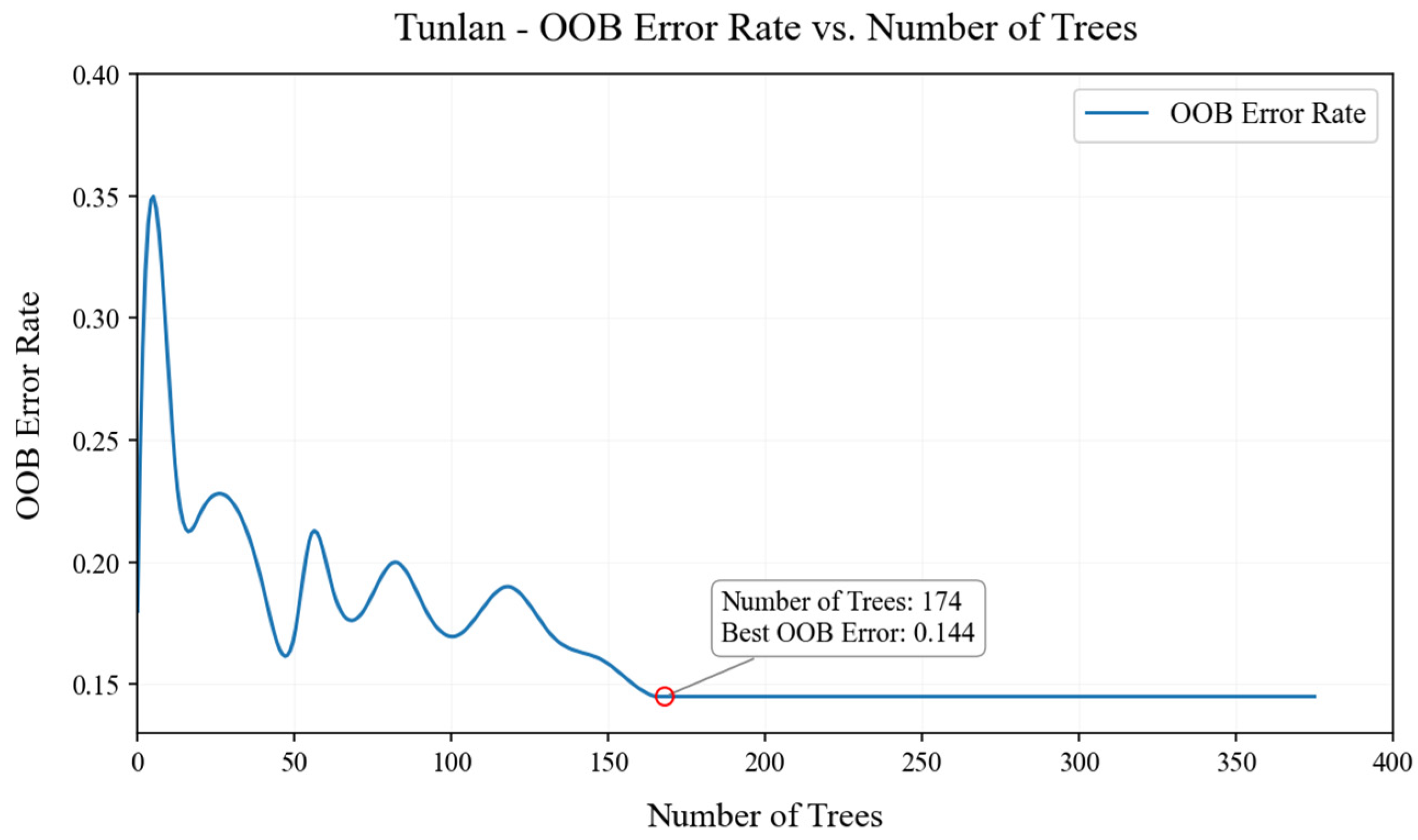
The random forest model constructed in this study is based on a mine water inrush source dataset comprising 128 samples in total. For random forest, a larger number of trees is generally preferable [31]. However, an excessive number of decision trees prolongs model prediction time and increases resource consumption, necessitating parameter tuning to achieve a balance between model performance and accuracy. The initial number of decision trees was set to 400; after parameter tuning and pruning, the final number of decision trees (weak learners) was determined to be 383. Upon completion of model training, the final OOB error rate was calculated as 0.144 (i.e., 14.4%). The relationship between OOB error rate with the number of trees can be seen in Figure 5.

The OOB error rate shows that the model achieves 85.6% accuracy on out-of-bag samples that were not used when building the trees. This indicates that the model generalizes well and can reliably classify unknown water source samples in this multi-class setting. From Figure 5, the OOB error changes with the number of trees at first: it can rise in the early stage, then fall as more trees are added. Before about 174 trees the error still fluctuates; with further increase in tree number and after pruning, it stabilizes at 14.4%. The chosen number of 383 trees therefore balances low error, stable performance, and acceptable computation time, and keeps hardware requirements manageable. Together, these results support the reasonableness of the random forest model built on the Tunlan Mine data.

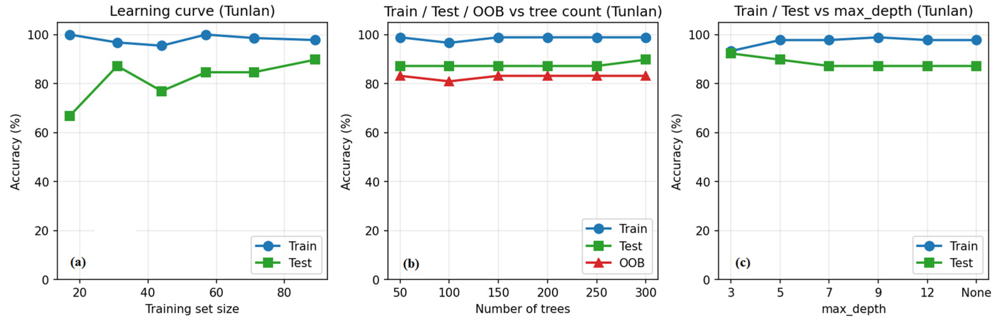
To assess whether the random forest model is overfitting, Figure 6 presents training, test, and out-of-bag (OOB) accuracies and provides three diagnostic plots for the Tunlan case. Figure 6a shows the learning curve: as the training set size increases (20% to 100%), test accuracy rises to about 90% without the typical overfitting pattern of rising training and falling test accuracy. Figure 6b shows Train, Test, and OOB accuracy versus the number of trees (50–300): Train > Test > OOB, and test accuracy does not decrease with more trees. Figure 6c shows Train and Test accuracy versus max_depth (3, 5, 7, 9, 12, None): test accuracy is highest at max_depth = 3 (92.31%) and decreases slightly for deeper trees, consistent with moderate pruning benefiting generalization. Together, these results indicate that the random forest model on the Tunlan data is not severely overfit and that the reported test performance is a reasonable reflection of generalization.

3. Results

3.1. Model Performance Comparison in the Single-Mine Scenario

3.1.1. Discrimination Accuracy Test

To examine the baseline performance of the improved fisher discriminant model and the random forest model in water source identification at the Tunlan Mine, this study employed the resubstitution method to test discrimination accuracy for both algorithms. Suppose n samples are selected from the total dataset and classified using the established model. If k samples are misclassified, the accuracy η is calculated as [32]:

$$\eta = {\displaystyle \frac{n -k}{n}}$$

(8)

where (n) is the total number of samples in the test set, and (k) is the number of samples that are misclassified by the model. $\eta$ represents the proportion of correctly classified samples.

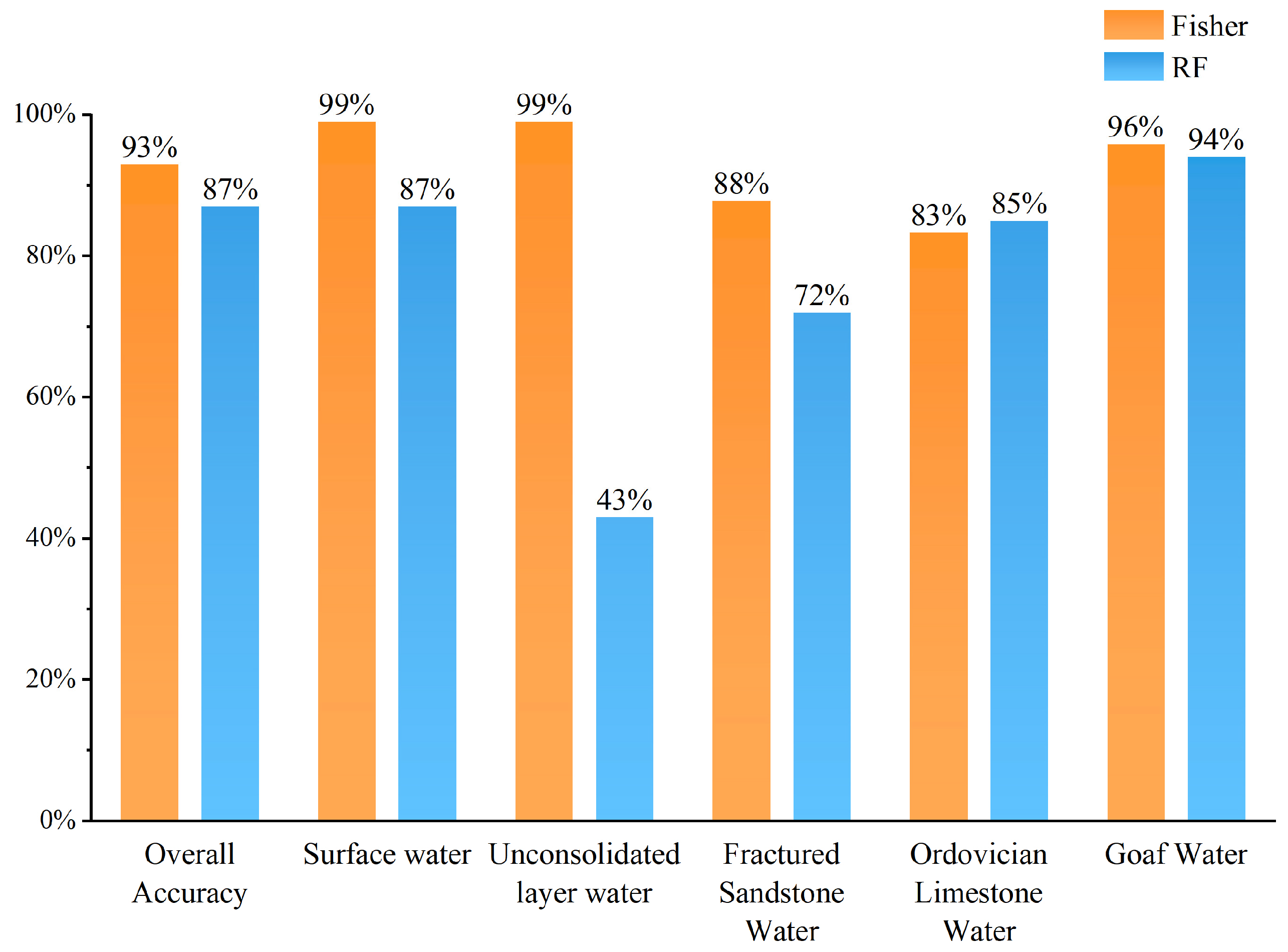
The results indicate that both algorithms exhibit strong discrimination capabilities, although significant performance differences exist. The specific discrimination accuracy results are presented in Figure 7 below.

The improved Fisher algorithm achieves a discrimination accuracy of 93% on the Tunlan Mine dataset. In contrast, the random forest algorithm yields an overall discrimination accuracy of 87% on the same dataset.

By water source type, the Fisher algorithm outperforms random forest in accuracy for most categories, except for Ordovician limestone water and goaf water, where accuracies are similar. For Permian sandstone fissure water, both algorithms show lower accuracies, but the gap narrows compared to the previous categories.

3.1.2. Confusion Matrix

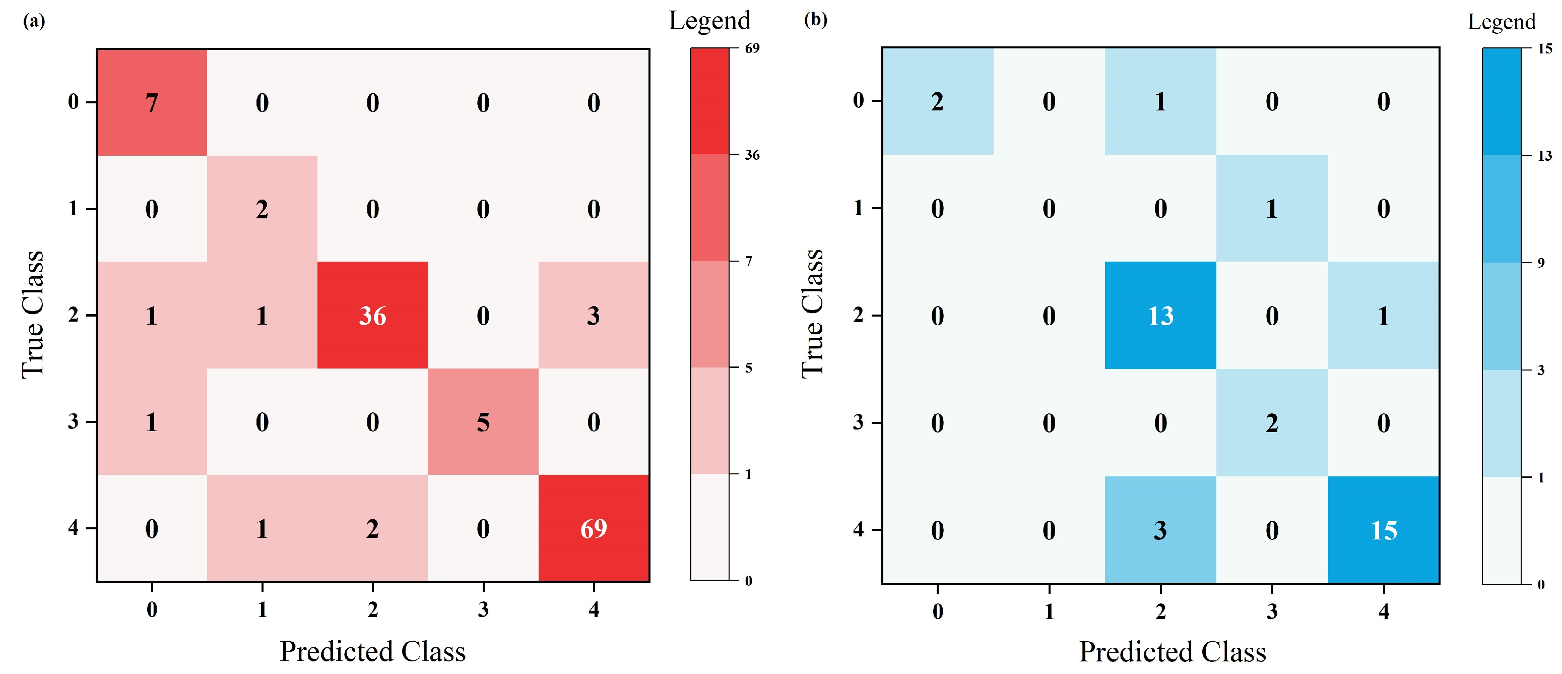
For the discrimination data and results, 5 × 5 confusion matrices are constructed separately for Fisher and random forest (Figure 8), providing an intuitive display of the performance of the two models. The confusion matrix compares predicted results with actual labels: columns represent the true water sample categories (vertical), and rows represent the predicted categories (horizontal). Categories from 0 to 4 correspond sequentially to surface water, unconsolidated layer water, Permian sandstone fissure water, Ordovician limestone water, and goaf water.

Values on the main diagonal indicate correct predictions where the predicted category matches the true category. Off-diagonal values represent misclassified samples.

For the Fisher algorithm, all surface water and unconsolidated layer water samples are correctly classified with no misclassifications. 36 samples are correctly identified, while 4 are misclassified (1 as surface water, 1 as unconsolidated layer water, and 3 as goaf water), yielding an accuracy of 90%. For Ordovician limestone water, one sample is misclassified as surface water. For goaf water, one sample is misclassified as unconsolidated layer water and two as sandstone fissure water.

For the random forest algorithm, one surface water sample is misclassified as Permian sandstone fissure water. Among Permian sandstone fissure water samples, 13 are correctly classified, but one is misclassified as goaf water. All three goaf water samples are misclassified as Permian sandstone fissure water.

3.1.3. Precision, F1-Score, and Recall

To further evaluate the comprehensive performance of Fisher discriminant analysis and random forest in the mine water source classification task, precision, recall, and F1-score are calculated based on the confusion matrix. Precision is the probability that samples predicted as positive are truly positive, calculated as Precision = TP/(TP + FP). Recall is the probability that true positive samples are predicted as positive and calculated as Recall = TP/(TP + FN). The F1-score is the harmonic mean of precision and recall, providing a comprehensive measure of classification performance: F1 = (2 × Precision × Recall)/(Precision + Recall). The calculated metrics for Fisher and random forest are listed in

Table 2. Comparison of metrics between Fisher discriminant method and random forest.

Metric	Fisher Discriminant Method	Random Forest
Precision	0.94	0.84
Recall	0.93	0.84
F1-score	0.93	0.83

below.

As shown in Table 2, the Fisher discriminant method achieves a precision of 0.94, recall of 0.93, and F1-score of 0.93, while the corresponding values for random forest are 0.84, 0.84, and 0.83.

3.1.4. Feature Importance Analysis

(1)

Feature Contribution in Fisher for Each Sample

To deeply analyze the relative contribution of each hydrochemical indicator to model classification decisions, the absolute values of coefficients in the Fisher discriminant functions are compared to reflect the contribution of each feature to the corresponding function. However, for the overall discrimination process, direct coefficient comparison is influenced by feature scales, and different discriminant functions contribute variably to the total discrimination. Therefore, features are standardized on a common scale. In this study, the variance contribution rates of each discriminant function (0.6098, 0.2176, 0.1705, 0.0021) are used as weights for weighted standardization. The coefficients for each feature across the four discriminant functions are:

Discriminant function 1: [−0.0630, 0.2422, −0.1334, 0.1428, −0.9464, 0.0305, −0.0364, 0.0365]; discriminant function 2: [0.3850, −0.5584, −0.3349, 0.2302, 0.2200, −0.5420, −0.0193, 0.1796]; discriminant function 3: [0.7385, 0.0837, 0.0896, −0.0863, 0.5161, −0.0558, −0.3553, −0.1909]; discriminant function 4: [0.1950, −0.1237, −0.2792, 0.2177, 0.2965, −0.2985, −0.6465, −0.4758].

The corresponding feature order is: X₁: total hardness; X₂: pH; X₃: K⁺; X₄: K⁺%; X₅: Na⁺%; X₆: Cl⁻%; X₇: SO₄²⁻; X₈: HCO₃⁻%.

$${\sum }_{i=0}^n{{\mathsf{\lambda }}_{\mathrm{i} }\ast \left({\mathsf{\omega }}_{\mathrm{i}}\right)}^2$$

(9)

Feature importance is calculated as follows: (9) where i denotes each feature, λ_i is the variance contribution rate of each discriminant function, and ω_i is the factor coefficient in each discriminant function.

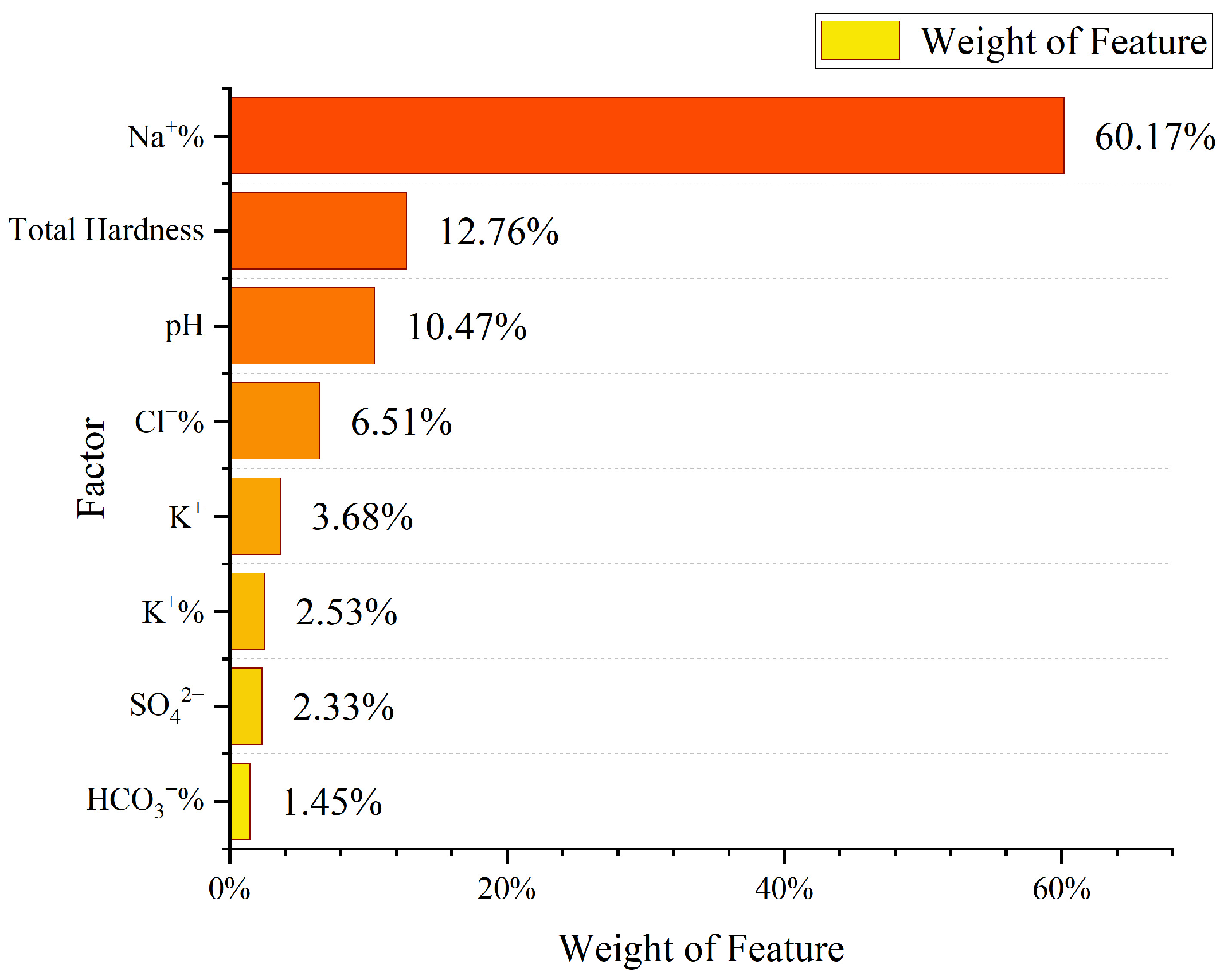
After calculating feature importance and normalization, the contribution of each factor is shown as Figure 9 below.

Comparison of factor feature importance in Fisher reveals the following ranking from highest to lowest: Na⁺% > total hardness > pH > Cl⁻% > K⁺ > K⁺% > SO₄²⁻ > HCO₃⁻%. Among these, the percentage content of sodium ions (Na⁺%) is the key indicator, contributing 60.17% to discrimination.

(2)

Feature Importance of Each Factor in Random Forest

For the random forest model, feature importance is assessed based on the mean decrease in Gini index. The Gini index measures node purity in decision trees, with lower values indicating more concentrated class distributions within nodes. Feature importance is calculated from the Gini index decrease, essentially reflecting the average contribution of a feature to reducing data impurity across all node splits in the random forest trees.

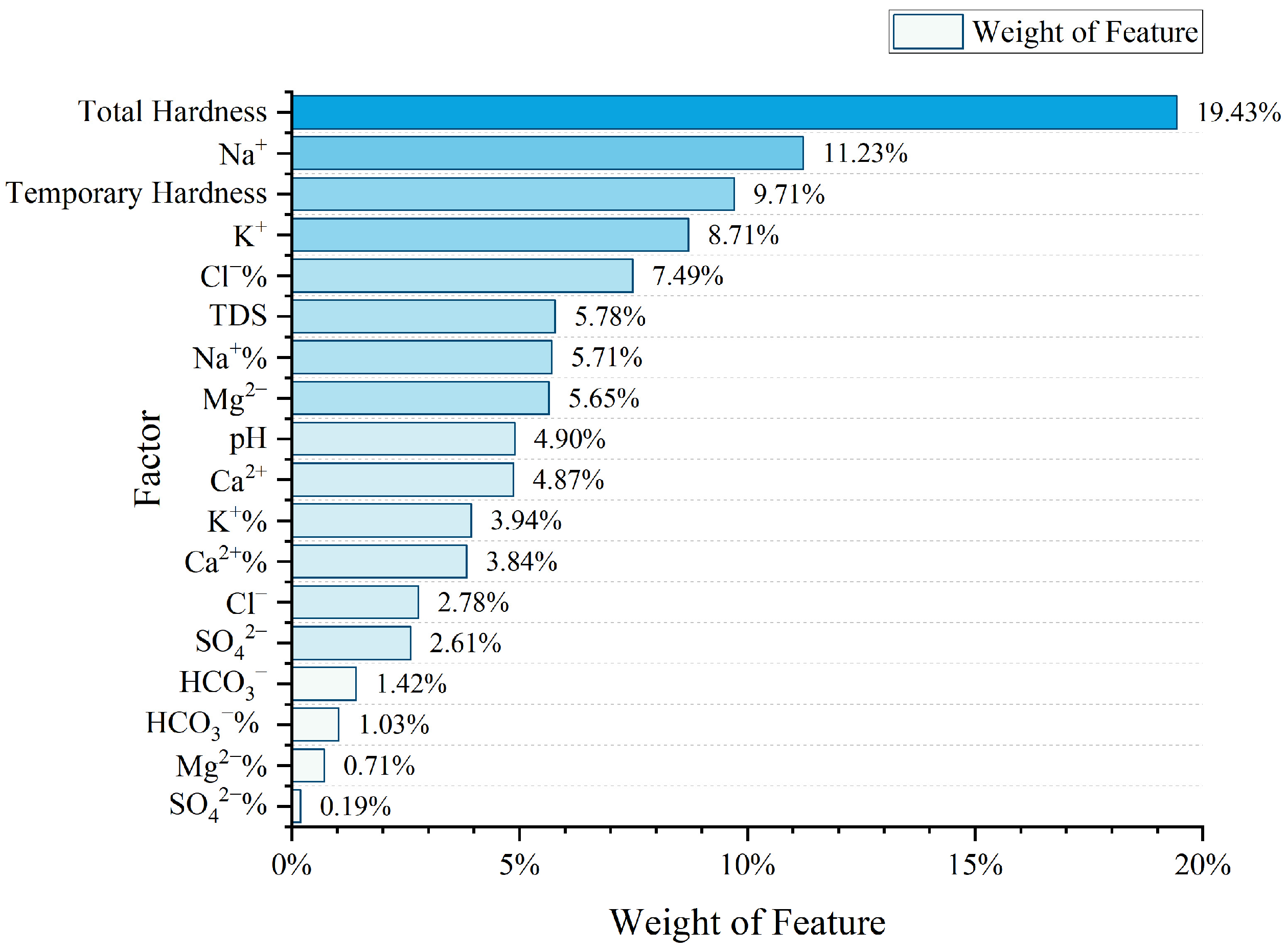
For comparability, feature importance is presented in percentage form in both methods: in Fisher (Figure 9) by construction; in the random forest (Figure 10) by normalizing each feature’s mean decrease in Gini to the total (sum = 100%).

Higher values indicate that the feature is more frequently used for effective node splitting and plays a more significant role in distinguishing mine water categories. The ranking of feature importance for each factor is presented in Figure 10 below.

Analysis indicates that total hardness, Na⁺, K⁺, temporary hardness, and Cl⁻% exhibit higher feature importance in the discrimination process, collectively accounting for 56.6% of the total importance as the primary indicators for mine water classification.

3.2. Generalization Ability Evaluation in Multi-Mine Joint Discrimination Scenarios

3.2.1. Necessity of Joint Discrimination

In practical water inrush identification processes, situations often arise where the number of samples from certain aquifers in the study area is limited or the overall mine water samples are insufficient. This may occur in newly developed coal mines or due to inadequate sample collection. Such conditions pose challenges for mine water inrush source identification, as model generalization ability is closely related to the quantity and quality of training samples. When sample sizes for certain categories or mines are too small, direct model training on such data fails to adequately constrain and optimize model parameters, resulting in a risk of overfitting. This leads to unstable performance on unknown samples and a sharp decline in generalization capability.

To address this issue, a joint discrimination approach can be adopted, integrating data from the mine with surrounding mines for categories or areas with insufficient samples. Within the same spring domain, aquifers with similar geological structures and recharge-runoff-discharge conditions typically have hydrochemical characteristics controlled by uniform physical-chemical processes. This implies that spatially adjacent mines may exhibit similar hydrogeochemical features for the same aquifer type. Therefore, integrating data from multiple mines with similar hydrogeological conditions and spatial proximity is feasible and reasonable. Joint discrimination expands the training set size, mitigating overfitting risks associated with small-sample modeling, while facilitating the construction of a more stable water source identification model that better represents the overall characteristics of a regional aquifer type, thereby enhancing the robustness and reliability of statistical models and compensating for deficiencies in single-mine sample availability.

3.2.2. Multi-Mine Experimental Results

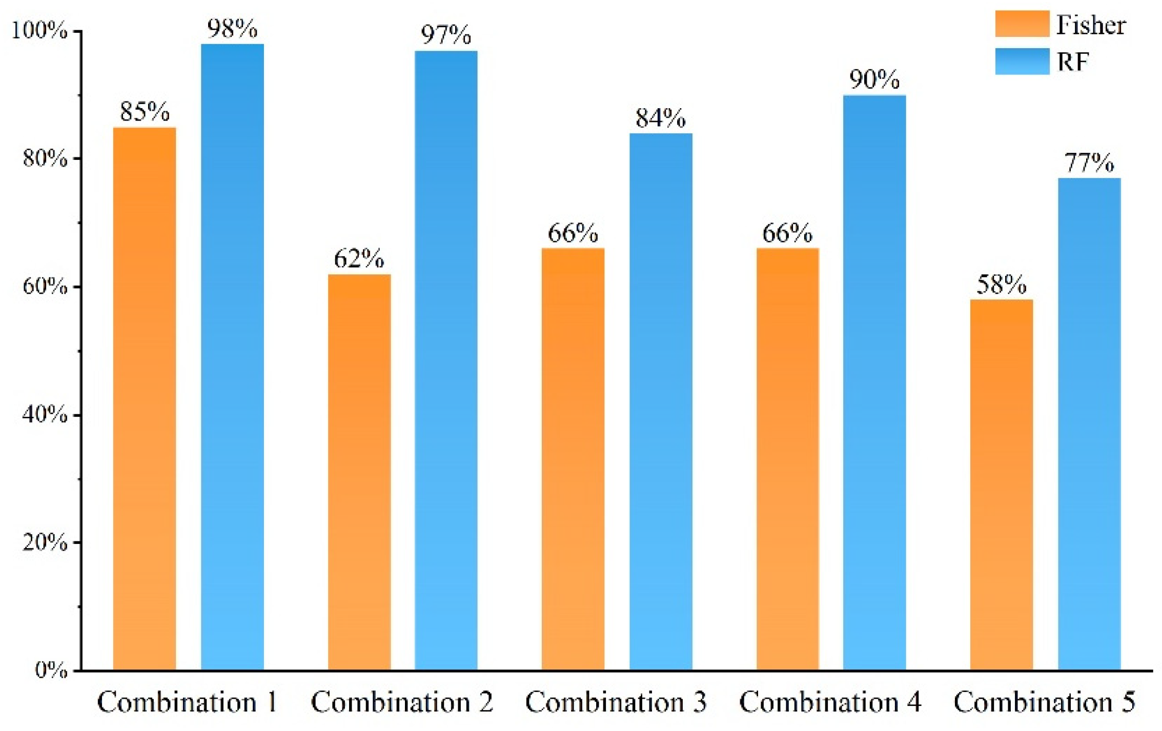
To verify the applicability and performance of Fisher discriminant analysis and random forest algorithms in regional joint discrimination, this study selected multiple mines from the Jinci Spring domain (including Bolong, Fuchang, Malan, and Liaoyuan) along with surrounding areas in Taiyuan City, such as the Liulin Spring domain, Longzi Spring domain, and Lanhe river system, forming five different mine combinations for modeling and testing. Combination 1 is the Longzi Spring domain (Guangdao and Shenghui mines), Combination 2 is the Lanhe river system (Sanjusheng and Majiayan mines), Combination 3 is Bolong and Fuchang mines, Combination 4 is Bolong, Fuchang, and Malan mines, and Combination 5 is Bolong, Fuchang, Malan, and Liaoyuan mines. The results of joint discrimination using Fisher and random forest across different mine combinations are presented in Figure 11.

From the joint discrimination results, across the five mine combination scenarios, the random forest model consistently and significantly outperforms the Fisher algorithm in classification accuracy. Its accuracy fluctuates within a narrow range (77–98%), demonstrating strong robustness. Particularly in the Longzi Spring domain and Lanhe river system, random forest achieves accuracies of 98% and 97%, respectively, not only proving its powerful generalization ability in multi-mine joint data discrimination but also indicating its effectiveness in learning and discriminating based on nonlinear patterns with discriminative power across different hydrogeological units.

In contrast to the stable performance of random forest, the Fisher algorithm exhibits greater accuracy fluctuations (58–85%) and generally lower overall accuracies. This reveals the limitations of Fisher as a linear model, where classification performance primarily depends on the degree of linear separability in the data distribution. For single-mine water source data, samples exhibit a favorable linear distribution, leading to superior performance over random forest. However, merging data from multiple mines increases sample source diversity and data complexity, rendering the hydrochemical feature space more intricate and making linear discriminant boundaries ineffective in separating categories, resulting in significant accuracy decline.

3.3. Linearity and Nonlinearity of Single-Mine vs. Multi-Mine Datasets

In the single-mine scenario, the improved Fisher discriminant analysis achieves higher discrimination accuracy than random forest (93% vs. 87%), whereas in multi-mine joint discrimination, random forest consistently outperforms Fisher. To understand what causes this difference in performance—i.e., why a linear model (Fisher) excels in one setting and a nonlinear ensemble (random forest) in the other—this study examines whether the underlying data structure differs in terms of linear versus nonlinear separability between single-mine and multi-mine datasets.

To provide independent evidence for whether single-mine data are more linearly separable than multi-mine joint data, the same datasets in Section 3.2 were evaluated by using indicators: (1) linear-kernel SVM 5-fold cross-validation accuracy (%), (2) LDA leave-one-out (LOO) accuracy (%), and (3) the support vector (SV) fraction (%) when fitting the linear SVM. Higher linear SVM or LDA accuracy indicates that a linear decision boundary separates the classes well; a lower SV fraction indicates that fewer samples define the boundary, and the data are more linearly separable. Results are given in

Table 3. SVM-based indicators of linearity and nonlinearity by dataset.

Dataset	Type	Linear SVM (%)	LDA LOO (%)	SV Fraction (%)
Tunlan	Single	86.96	92.17	26.96
Lanhe river system	Multi-mine joint	61.90	61.29	77.42
Bo-Ma-Fu	Multi-mine joint	80.87	86.18	44.72
Longzi Spring domain	Multi-mine joint	80.00	84.62	40.00

.

As shown in Table 3, the single-mine Tunlan dataset has the highest linear SVM 5-fold accuracy (86.96%) and the highest LDA·LOO accuracy (92.17%), and the lowest SV fraction (26.96%). This indicates that the single-mine feature space is well separated by a linear boundary and that a relatively small proportion of samples suffice to define it. Among the multi-mine joint datasets, the Lanhe river system shows the lowest linear performance (Linear SVM 61.90%, LDA·LOO 61.29%) and the highest SV fraction (77.42%), consistent with the greatest difficulty in linear separation. The Bo-Ma-Fu and Longzi Spring domain datasets show intermediate linear accuracies (Linear SVM 80–81%, LDA·LOO 84–86%) and moderate SV fractions (40–45%), which are higher than Tunlan’s but much lower than Lanhe’s. Thus, on average, multi-mine joint data exhibit lower linear SVM accuracy and higher SV fractions than the single-mine case, with Lanhe being the least linearly separable and Bo-Ma-Fu and Longzi Spring domain being relatively more linear among the multi-mine datasets but still with higher SV fractions than Tunlan.

4. Discussion

The results presented in Section 3 demonstrate a clear performance divergence between the improved Fisher discriminant analysis and the random forest model depending on the application scenario. In the single-mine setting (Tunlan), the linear Fisher algorithm (93% accuracy) outperforms the nonlinear ensemble method (87% accuracy), whereas in multi-mine joint discrimination, random forest consistently achieves higher accuracies (77–98%) than Fisher (58–85%). This contrast suggests that the underlying data structure—specifically the degree of linear separability—plays a decisive role in model suitability.

To verify this hypothesis independently of the Fisher and random forest models, we examined two additional linearity indicators: linear SVM accuracy and the fraction of support vectors that exhibit nonlinear behavior, together with the linear discriminant analysis (LDA) leave-one-out accuracy (Table 3). For the single-mine Tunlan dataset, the high linear SVM and LDA accuracies combined with a low SV fraction (26.96%) confirm that the hydrochemical classes are well separated by a linear boundary and that this boundary is defined by only a few critical samples. This directly supports the strong performance of the improved Fisher algorithm in the single-mine scenario.

In contrast, all multi-mine joint datasets exhibit lower linear SVM and LDA accuracies and substantially higher SV fractions than Tunlan. The Lanhe river system, where Fisher accuracy drops to 62%, is the least linearly separable: it has the lowest linear SVM accuracy, the lowest LDA accuracy, and the highest SV fraction (77.42%), indicating that most samples lie near the decision boundary and the class structure is inherently complex. The Bo-Ma-Fu and Longzi Spring domain datasets, although more linear than Lanhe (SV fractions of 44.72% and 40.00%, respectively), still show SV fractions markedly higher than Tunlan’s 26.96%, reflecting a more intricate or less easily separable feature space than in the single-mine case. These independent linearity measures align perfectly with the observed model performances: Fisher excels when data are strongly linear, while random forest maintains robustness across the more complex, less separable multi-mine datasets.

In the following subsections, we therefore delve deeper into the reasons behind these scenario-dependent outcomes. Section 4.1 analyses the single-mine case, focusing on why Fisher outperforms random forest when linear separability is high. Section 4.2 examines the multi-mine joint discrimination, exploring how hydrogeological similarity, spatial location, and the inherent nonlinearity of the data govern the superiority of random forest. Together, these discussions substantiate the recommendation that algorithm selection should be guided by the linearity characteristics of the data—a principle that balances interpretability, predictive accuracy, and practical applicability in mine water inrush source identification.

4.1. Single-Mine Scenario: Causes of Performance Difference

In the single-mine scenario, the improved Fisher algorithm reached 93% discrimination accuracy, indicating that its built-in factor selection identified a feature set well suited to the Tunlan Mine hydrogeology. The hydrochemical data in the selected feature space are largely linearly separable, so Fisher’s objective of maximizing between-class and minimizing within-class distance is well matched. Random forest achieved 87% accuracy, still showing solid classification ability; its lower performance may be due to limited sample size and a data structure that is predominantly linear, where nonlinear and ensemble mechanisms bring limited gain. By water source type, surface water and unconsolidated layer water have relatively simple, linearly separable hydrochemistry, which Fisher exploits effectively. Random forest’s low accuracy for unconsolidated layer water is likely due to the very small number of samples (two), which hinders its multi-feature and ensemble learning. Permian sandstone fissure water is harder for both models because of feature overlap with goaf water and weaker linear separability. In short, Fisher performs better where linear separation dominates; random forest is more suited to settings with stronger nonlinearity or more complex feature structure.

Misclassifications concentrate between Permian sandstone fissure water and goaf water, consistent with possible hydraulic connectivity or overlapping hydrochemistry between these sources. This supports the result that confusion between these two types is the main error pattern in both models. Fisher outperforms random forest on precision, recall, and F1-score (Table 2), indicating higher accuracy and stability for Tunlan water source classification, in line with its improved factor selection and explicit linear discriminant functions. Random forest’s weaker performance may be due to sensitivity to redundant or overlapping features (e.g., Permian sandstone vs. goaf similarity) and to limited generalization with small samples and fuzzy class boundaries. The random forest OOB error of about 14% still reflects reasonable discriminative ability, and its nonparametric form remains useful for more complex, nonlinear data; future work could include feature engineering, hyperparameter tuning, or other ensemble designs.

Feature importance differs between Fisher and random forest because of model design. Fisher is linear and uses only linear feature–class relations; when a feature like Na⁺% is strongly linearly discriminative, it dominates and other features contribute less. Random forest importance is based on mean Gini decrease over tree splits, with bootstrap and random feature subsets reducing the dominance of one variable and allowing nonlinear and interaction effects. Features with weak linear discriminability can still matter in combination, leading to a more balanced importance profile in random forest. In Fisher, Na⁺% is the dominant indicator, matching its strong linear separability across sources (low in surface and unconsolidated layer water, higher in Permian sandstone fissure water and goaf water). In random forest, total hardness, Na⁺, K⁺, and proportional terms such as Cl⁻% and Na⁺% form the core of the discrimination system, reflecting clear differences in hardness and relative ion balance among aquifers.

4.2. Multi-Mine (Joint) Scenario: Causes of Performance Difference

4.2.1. Analysis Based on Hydrochemical Data from Each Mine Area

In joint discrimination for the Longzi Spring domain and Lanhe river system, the random forest model achieves the highest accuracies of 98% and 97%, respectively. The Fisher algorithm attains its own best performance of 85% in the Longzi Spring domain but drops markedly to 62% in the Lanhe river system. To investigate the underlying reasons, Fisher discriminant ratio (FDR) and SVM classification margin are employed for quantitative evaluation. The FDR directly reflects the ratio of inter-class separation to intra-class dispersion; higher values indicate stronger linear separability. Results show an FDR of 0.49 for the Longzi Spring domain, 93% higher than the 0.25 for the Lanhe river system, confirming significantly superior inter-class separation in the former. Empirically, FDR > 0.5 is considered excellent; 0.2 < FDR ≤ 0.3 indicates that linear models are marginally usable with feature selection. The linear SVM classification margin (minimum Euclidean distance from support vectors to the separating hyperplane) is 130.03 in the Longzi Spring domain versus only 1.14 in the Lanhe river system—a 114-fold difference—indicating that the five water sources in the Lanhe river system are nearly adherent in chemical feature space. The number of support vectors (28 and 32, respectively) further indicates that nearly 90% of samples (32/36) in the Lanhe river system lie near classification boundaries, exhibiting poor robustness for linear discrimination. LDA stability assessed by leave-one-out cross-validation (LOOCV) gives accuracy in the Longzi Spring domain (0.62 ± 0.01) significantly higher than in the Lanhe river system (0.52 ± 0.21); the high standard deviation in the latter suggests that adding or removing a few samples dramatically alters projection directions, confirming nonlinear fragility in its data structure. Overall, the Lanhe river system data are comprehensively inferior in linear separability compared to the Longzi Spring domain, which directly caps Fisher’s performance (62%), whereas random forest maintains 97% accuracy through ensemble nonlinear decision trees.

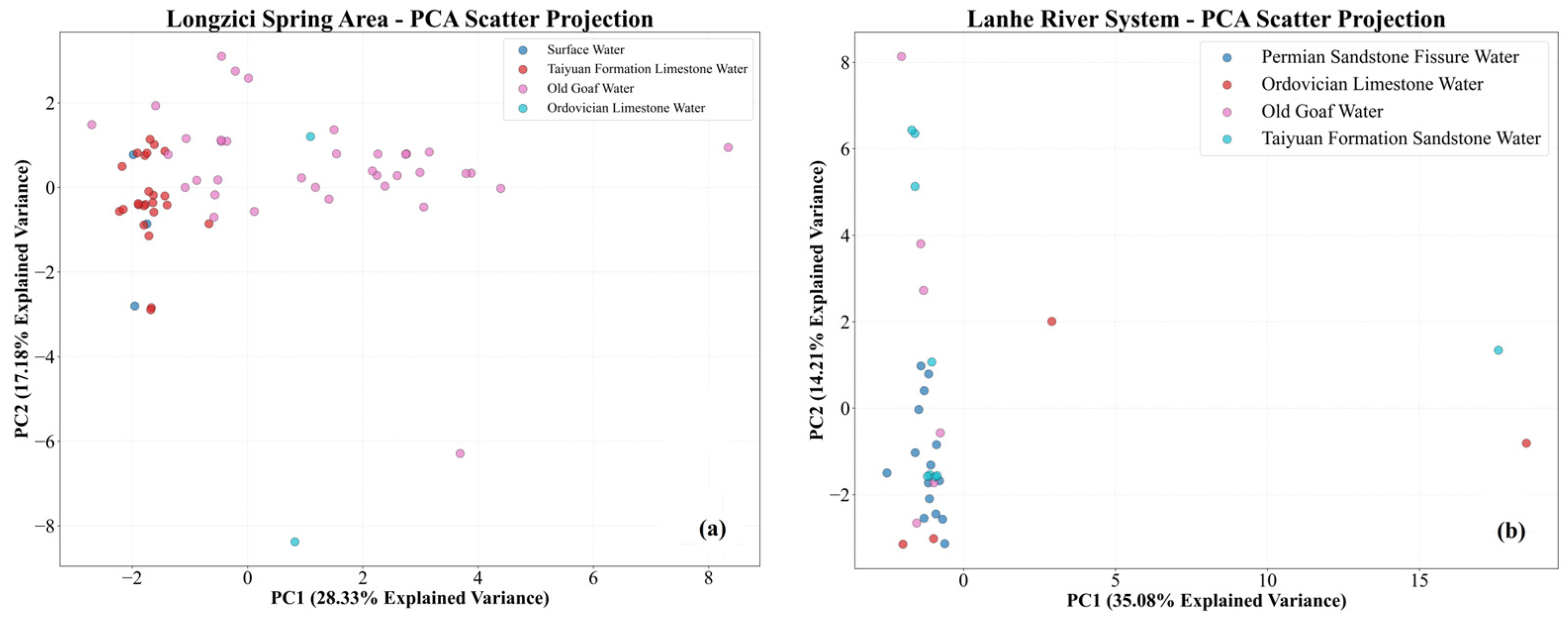
For intuitive visualization, PCA projection analysis is performed (Figure 12) for the Longzi Spring domain and Lanhe river system. PCA retains the first two principal components (PC1 and PC2) to display sample distribution in a reduced linear space.

In the Longzi Spring domain, four water sources (surface water, Taiyuan Formation limestone water, goaf water, and Ordovician limestone water) show roughly separable clusters in the PC1–PC2 plane, consistent with clear inter-class separability and Fisher’s relatively high accuracy (85%). Random forest further optimizes decision boundaries and reaches 98% accuracy. In contrast, the Lanhe river system PCA plot shows mixed and overlapping points, with no clear category boundaries in the PC1–PC2 plane. Fisher cannot find effective linear directions for separation, while random forest captures nonlinear patterns not visible in PCA and achieves 97% accuracy. The Longzi Spring domain and Lanhe river system are independent hydrological systems with internally consistent recharge–runoff–discharge processes. Joint modeling within each system yields datasets with modest sample sizes but concentrated intra-category distributions; when linear separability is strong, Fisher performs well, and when nonlinearity dominates, its performance deteriorates while random forest remains robust. These results indicate that joint discrimination can address single-mine sample insufficiency, but high-accuracy classification relies on the independence of hydrogeological units and internal consistency of the dataset.

4.2.2. Analysis Based on Spatial Location and Hydrogeological Environment

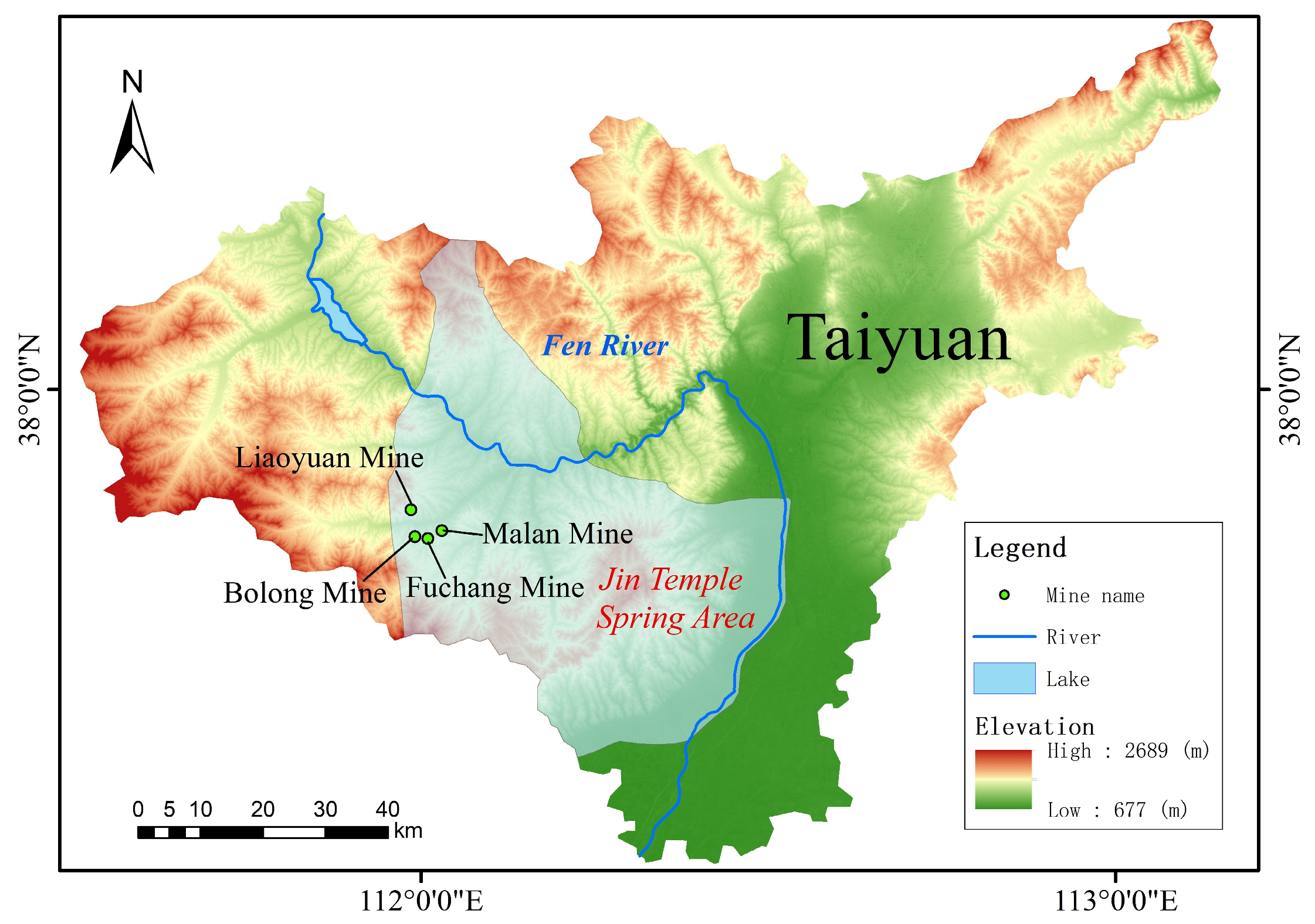
Examining model performance in combinations of Bolong, Fuchang, Malan, and Liaoyuan mines reveals no simple positive correlation between discrimination accuracy and sample size. From the “Bo-Ma” combination to “Bo-Ma-Fu,” random forest accuracy increases from 84% to 90% with data expansion; however, in the largest-sample “Bo-Ma-Fu-Liao” combination, accuracies for both Fisher and random forest decline markedly to 58% and 77%, respectively. This indicates that although adding Liaoyuan mine data expands the training set numerically, its hydrogeochemical characteristics significantly differ from the original “Bo-Ma-Fu” distribution. Spatially, Bolong, Fuchang, and Malan mines are located on the same side of a mountain range in an upstream–downstream continuum (Figure 13), implying tight spatial association and similar or interconnected hydrogeological units, potentially receiving common-source recharge and undergoing similar water–rock interactions.

In contrast, Liaoyuan mine lies on the opposite side of the mountain, where the topographic divide implies a different local hydrological system, leading to systematic deviations in hydrochemical features from the “Bo-Ma-Fu” combination. Incorporating Liaoyuan data thus introduces a subsample from another hydrogeochemical background, disrupting the consistent feature-space structure and degrading performance for both models: Fisher’s linear assumption is violated, and random forest’s decision boundaries become less generalizable. In summary, model effectiveness depends on data quality—whether the joint dataset forms a feature space with consistent distribution and high inter-class separability—rather than on cumulative sample quantity alone. In future construction of regional water source identification models, spatial geographic information such as mine topography, landforms, and hydrological system zoning should serve as critical criteria for data screening and dataset construction. Joint discrimination demonstrates that random forest, by handling nonlinear relationships, exhibits superior robustness and accuracy in most joint scenarios and is the preferred choice for regional models; Fisher performs well only when data are approximately linearly separable.

5. Conclusions

(1)

In the single-mine scenario, the improved Fisher discriminant analysis achieves an overall accuracy of 93%, significantly higher than the 87% accuracy of the random forest; its advantage lies in effectively exploiting linearly separable features in the data, making it particularly suitable for situations where hydrochemical indicators exhibit high linear separability.

(2)

In multi-mine joint discrimination scenarios, random forest maintains consistently stable accuracies of 77–98%, substantially outperforming the Fisher algorithm (58–85%), demonstrating greater robustness and generalization ability in handling complex nonlinear data distributions.

(3)

Model performance is primarily governed by data quality, feature distribution, and hydrogeological similarity rather than solely by sample size; indiscriminately merging data with substantial differences in hydrogeological backgrounds introduces noise and degrades performance.

(4)

Algorithm selection should be scenario-dependent: the improved Fisher discriminant analysis is preferred for single-mine applications or when linear features dominate; random forest is recommended for regional-scale, multi-mine joint discrimination or when nonlinear features are prominent. In practice, this scenario-dependent selection helps balance interpretability, data requirements, and predictive robustness when designing monitoring and early-warning workflows.

References

1. Xie, K.C. Strategy Research on Clean, High-Efficiency and Susta-Inable Coal Development and Utilization in China; China Science Publishing & Media Ltd. (CSPM): Beijing, China, 2014. [Google Scholar]
2. Peng, S.P. Research on Development Strategy of Great Power of Coal Resources; China Science Publishing & Media Ltd. (CSPM): Beijing, China, 2018. [Google Scholar]
3. Wang, D.; Sui, W.; Ranville, J.F. Hazard identification and risk assessment of groundwater inrush from a coal mine: A review. Bull. Eng. Geol. Environ. 2022, 81, 421. [Google Scholar] [CrossRef]
4. Zeng, Y.; Wu, Q.; Zhao, S.; Miao, Y.W.; Zhang, H.; Mei, A.S.; Meng, S.H.; Liu, X.X. Characteristics, causes, and prevention measures of coal mine water hazard accidents in China. Coal Sci. Technol. 2023, 51, 1−14. [Google Scholar] [CrossRef]
5. Yin, S.; Wang, Y.; Li, W. Cause, countermeasures and solutions of water hazards in coal mines in China. Coal Geol. Explor. 2023, 51, 214−221. [Google Scholar] [CrossRef]
6. Dong, D.; Zhang, J. Discrimination Methods of Mine Inrush Water Source. Water 2023, 15, 3237. [Google Scholar] [CrossRef]
7. Wu, Q.; Mu, W.; Xing, Y.; Qian, C.; Shen, J.; Wang, Y.; Zhao, D. Source discrimination of mine water inrush using multiple methods: A case study from the Beiyangzhuang Mine, Northern China. Bull. Eng. Geol. Environ. 2019, 78, 469–482. [Google Scholar] [CrossRef]
8. Bi, Y.; Wu, J.; Zhai, X.; Wang, G.; Shen, S.; Qing, X. Discriminant analysis of mine water inrush sources with multi-aquifer based on multivariate statistical analysis. Environ. Earth Sci. 2021, 80, 144. [Google Scholar] [CrossRef]
9. Sun, F.; Wei, J.; Wan, Y.; Liu, C. Recognition method of mine water source based on Fisher’s discriminant analysis and centroid distance evaluation. COAL Geol. Explor. 2017, 45, 80–84. [Google Scholar] [CrossRef]
10. Dong, D.; Chen, Z.; Lin, G.; Li, X.; Zhang, R.; Ji, Y. Combining the Fisher Feature Extraction and Support Vector Machine Methods to Identify the Water Inrush Source: A Case Study of the Wuhai Mining Area. Mine Water Environ. 2019, 38, 855–862. [Google Scholar] [CrossRef]
11. Li, B.; Xiang, X.; Wu, Q.; Wang, J.; Zeng, Y.; Li, T. Comparison of multiple methods for identifying water sources of mine water inrush and quantitative analysis of mixed water sources based on isotope theory. Earth Sci. Inform. 2025, 18, 26. [Google Scholar] [CrossRef]
12. Qian, J.; Tong, Y.; Ma, L.; Zhao, W.; Zhang, R.; He, X. Hydrochemical Characteristics and Groundwater Source Identification of a Multiple Aquifer System in a Coal Mine. Mine Water Environ. 2018, 37, 528–540. [Google Scholar] [CrossRef]
13. Huang, P.; Yang, Z.; Wang, X.; Ding, F. Research on Piper-PCA-Bayes-LOOCV discrimination model of water inrush source in mines. Arab. J. Geosci. 2019, 12, 234. [Google Scholar] [CrossRef]
14. Cui, M.; Huang, P.; Hu, Y.; Chai, S.; Zhang, Y.; Li, Y. Application of dynamic weight in coal mine water inrush source identification. Environ. Earth Sci. 2024, 83, 69. [Google Scholar] [CrossRef]
15. Lu, X.; Wang, Q.; Xie, B.; Zhu, J. A KPCA-ISSA-SVM Hybrid Model for Identifying Sources of Mine Water Inrush Using Hydrochemical Indicators. Water 2025, 17, 2859. [Google Scholar] [CrossRef]
16. Yang, Z.; Lv, H.; Xu, Z.; Wang, X. Source discrimination of mine water based on the random forest method. Sci. Rep. 2022, 12, 19568. [Google Scholar] [CrossRef] [PubMed]
17. Ma, X.; Yan, P.; Wang, K. Identification of mine water source by random forest combined with laser-induced fluorescence spectra. Front. Environ. Sci. 2024, 12, 1392496. [Google Scholar] [CrossRef]
18. Wang, M.; Zhang, J.; Li, H.; Zhang, B.; Yang, Z. Identification of mine water source based on TPE-LightGBM. Sci. Rep. 2024, 14, 12539. [Google Scholar] [CrossRef] [PubMed]
19. Yang, Z.; Li, H.; Wang, X.; Meng, H.; Xi, T.; Hou, Z. Source identification of mine water inrush based on GBDT-RS-SHAP. Environ. Earth Sci. 2025, 84, 114. [Google Scholar] [CrossRef]
20. Jiang, C.; Zhu, S.; Hu, H.; An, S.; Su, W.; Chen, X.; Li, C.; Zheng, L. Deep learning model based on big data for water source discrimination in an underground multiaquifer coal mine. Bull. Eng. Geol. Environ. 2022, 81, 26. [Google Scholar] [CrossRef]
21. Cui, M.; Hou, E.; Feng, D.; Che, X.; Xie, X.; Hou, P. Identification of the Water Inrush Source Based on the Deep Learning Model for Mines in Shaanxi, China. Mine Water Environ. 2025, 44, 133–148. [Google Scholar] [CrossRef]
22. Li, X.; Dong, D.; Liu, K.; Zhao, Y.; Li, M. Identification of Mine Mixed Water Inrush Source Based on Genetic Algorithm and XGBoost Algorithm: A Case Study of Huangyuchuan Mine. Water 2022, 14, 2150. [Google Scholar] [CrossRef]
23. Fang, B. Method for Quickly Identifying Mine Water Inrush Using Convolutional Neural Network in Coal Mine Safety Mining. Wirel. Pers. Commun. 2022, 127, 945–962. [Google Scholar] [CrossRef]
24. Wei, Z.; Dong, D.; Ji, Y.; Ding, J.; Yu, L. Source Discrimination of Mine Water Inrush Using Multiple Combinations of an Improved Support Vector Machine Model. Mine Water Environ. 2022, 41, 1106–1117. [Google Scholar] [CrossRef]
25. Zeng, Y.; Mei, A.; Wu, Q.; Meng, S.; Zhao, D.; Hua, Z. Double verification and quantitative traceability: A solution for mixed mine water sources. J. Hydrol. 2024, 630, 130725. [Google Scholar] [CrossRef]
26. Ju, Q.; Hu, Y.; Liu, Q. Grey Situation Decision Method Based on Improved Whitening Function to Identify Water Inrush Sources in the Whole Cycle of Coal Mining. Water 2025, 17, 1479. [Google Scholar] [CrossRef]
27. Li, Q.; Fan, G.; Zhang, D.; Yu, W.; Zhang, S.; Fan, Z.; Fu, Y. Novel Method on Mixing Degree Quantification of Mine Water Sources: A Case Study. Processes 2024, 12, 433. [Google Scholar] [CrossRef]
28. Fisher, R.A. The use of multiple measurements in taxonomic problems. Ann. Hum. Genet. 1936, 7, 179–188. [Google Scholar] [CrossRef]
29. Breiman, L. Random Forests. Mach. Learn. 2001, 45, 5–32. [Google Scholar] [CrossRef]
30. Qiao, W.; Li, W.; Zhang, S.; Niu, Y. Effects of coal mining on the evolution of groundwater hydrogeochemistry. Hydrogeol. J. 2019, 27, 2245–2262. [Google Scholar] [CrossRef]
31. Probst, P.; Anne-Laure, B. To tune or not to tune the number of trees in random forest? J. Mach. Learn. Res. 2018, 18, 1–18. [Google Scholar] [CrossRef]
32. Sokolova, M.; Lapalme, G. A systematic analysis of performance measures for classification tasks. Inf. Process. Manag. 2009, 45, 427–437. [Google Scholar] [CrossRef]
Figure 1. Location map of the Tunlan Mine.
Water 18 00711 g001
Figure 2. Stratigraphic column of the Tunlan Mine.
Water 18 00711 g002
Figure 3. Box plots of hydrochemical parameters for water samples from the Tunlan Mine. (a) pH; (b) Total hardness; (c) Mg2+; (d) Ca2+; (e) TDS; (f) SO42−; (g) Cl; (h) K+; (i) Na+.
Water 18 00711 g003
Figure 4. Correlation heat map between water source types and hydrochemical factors for the Tunlan Mine.
Water 18 00711 g004
Figure 5. Variation in random forest OOB error rate with the number of trees.
Water 18 00711 g005
Figure 6. Random forest learning curve and hyperparameter analysis on Tunlan dataset. (a) Learning curve: training and test accuracy versus training set size; (b) Train, test, and OOB accuracy vs. number of trees. (c) Train and test accuracy vs. max_depth.
Water 18 00711 g006
Figure 7. Comparison of accuracy between Fisher and random forest for the Tunlan Mine.
Water 18 00711 g007
Figure 8. Heat map of confusion matrices for Fisher (a) and Random forest (b).
Water 18 00711 g008
Figure 9. Feature importance of factors in the Fisher algorithm.
Water 18 00711 g009
Figure 10. Feature importance of each factor in the random forest algorithm for the Tunlan Mine.
Water 18 00711 g010
Figure 11. Comparison of accuracy between Fisher and random forest in joint discrimination.
Water 18 00711 g011
Figure 12. PCA projection plots for the Longzi Spring domain (a) and Lanhe river system (b).
Water 18 00711 g012
Figure 13. Location map of Bolong, Fuchang, Malan, and Liaoyuan mines.
Water 18 00711 g013