High-Accuracy Mangrove Extraction and Degradation Diagnosis Using Time-Series Remote Sensing and Deep Learning: A Case Study of the Largest Delta in the Northern Beibu Gulf, China

Abstract

Mangrove extent has increased in many regions under strengthened conservation policies and large-scale restoration programs. Nevertheless, mangrove ecosystems continue to face multiple pressures, including limited total area, habitat degradation, biodiversity decline, and biological invasion, and localized deterioration in ecosystem structure and function has been increasingly reported. Despite extensive mapping efforts, the spatiotemporal dynamics of mangrove degradation—particularly in tidally influenced environments—remain insufficiently understood. Focusing on the Nanliu River Delta, the largest deltaic mangrove system in the Northern Beibu Gulf of China, this study integrates long-term Landsat time-series imagery (1990–2025) with deep learning to quantify both mangrove extent change and canopy degradation. To mitigate tidal inundation effects, a NDVI Pseudo-P75 compositing strategy was applied using Google Earth Engine (GEE), enabling consistent observation of mangrove canopies across tidal stages. Global Mangrove Watch v4 (GMW-V4) and HGMF2020 mangrove dataset for China were used as reference labels to train a ResNet34–UNet segmentation framework incorporating Digital Elevation Model (DEM) constraints. The model achieved high classification performance, with an IoU of 0.822 for mangroves and 0.981 for background, yielding a mean IoU of 0.902. The resulting maps, following manual verification, provided a robust basis for spatiotemporal and degradation analyses. Canopy condition was further assessed using the Enhanced Vegetation Index (EVI), which is less prone to saturation in high-biomass mangrove stands. Results show that mangrove area in the Nanliu River Delta expanded from 266 ha in 1990 to 1414 ha in 2025, with the annual expansion rate after 2005 being nearly seven times higher than that before 2005. Despite this net gain, a cumulative loss of 347.45 ha was recorded, primarily during 1990–2000, with approximately 70% converted to aquaculture and coastal engineering. Spatial analysis revealed that mangrove expansion occurred predominantly seaward, whereas both mangrove loss and canopy degradation exhibited an inverse J-shaped relationship with seawall proximity. More than 80% of mangrove loss occurred within 200 m of seawalls, indicating concentrated anthropogenic encroachment, while 75.6% of canopy degradation was observed within 350 m, potentially reflecting landward forest senescence. These results indicate a transition in dominant threats from permanent land conversion in the late 20th century to more subtle, internal functional degradation in recent decades, underscoring the need to complement extent-based assessments with canopy condition monitoring in mangrove conservation and management.

1. Introduction

Mangroves are a typical coastal wetland ecosystem widely distributed across tropical and subtropical regions, playing a critical ecological role [1] in coastal protection [2,3], marine economy [4,5], and blue carbon sequestration [6,7]. However, over the past several decades, global mangrove forests have declined at an annual rate of 0.16–0.39% [8], mainly due to intensive human activities—such as aquaculture expansion [9], land reclamation [10], and port construction, compounded by climate change and extreme events [11]. In China, historical estimates suggest that mangrove area declined substantially during the mid-to-late 20th century, and national surveys indicate that mangrove extent decreased from approximately 40,000–42,000 ha in the 1950s to 17,000–23,000 ha by the 1990s [12]. Mangrove conservation and restoration have become a major focus of the international community [13] and promoted a recent rebound [14]. Despite this recovery, many mangrove ecosystems continue to face degradation risks in terms of canopy structure, regeneration capacity, and ecosystem functioning, highlighting the need to shift management priorities from area expansion alone to quality-oriented restoration [15].

A clear conceptual distinction must be made between mangrove loss and mangrove degradation. In this study, loss refers to the complete conversion of mangrove forest to non-mangrove land cover (e.g., aquaculture, urban land, bare tidal flat), resulting in the disappearance of mangrove extent. In contrast, degradation denotes the persistence of mangrove cover accompanied by a decline in ecosystem condition, function, or productivity, without full land-cover conversion. Following established ecological frameworks, degradation may include structural degradation (e.g., canopy thinning, increased gap fraction), functional degradation (e.g., reduced biomass accumulation and stress tolerance), and productivity decline (e.g., reduced photosynthetic activity and vigor) [11,15]. These processes represent a loss of ecosystem quality even when mangrove extent remains unchanged. Despite this conceptual distinction, most remote-sensing studies still conflate mangrove loss with degradation, largely due to methodological limitations in intertidal environments.

Satellite remote sensing provides long-term, consistent, and spatially explicit information on mangrove distribution, forming the foundation for analyzing mangrove spatiotemporal dynamics and assessing loss. Remote sensing-based vegetation indices such as the Enhanced Vegetation Index (EVI) are widely used to diagnose such functional and physiological degradation, as they are sensitive to changes in canopy density, leaf area, and photosynthetic capacity. Among available sensors, Landsat imagery remains the cornerstone for such monitoring, offering a continuous historical coverage exceeding four decades [16,17]. Numerous studies have used Landsat time series to map mangrove extent and change at regional to global scales, including the Global Mangrove Watch initiative [18], national-scale mapping in China [19,20], Southeast Asia [21,22], and estuarine deltas worldwide [8]. These studies demonstrate the value of Landsat for mangrove long-term trend analysis, but they also reveal substantial uncertainties in intertidal environments where periodic inundation, turbidity, and mixed pixels complicate mangrove detection.

A key challenge arises from tidal contamination. First, periodic tidal inundation creates a spectral masking effect. When mangroves are submerged, the water’s great absorption of near-infrared (NIR) and shortwave-infrared (SWIR) signals drastically alters the vegetation signature. This leads to mixed pixels where the spectral response is a hybrid of canopy, turbid water, and mudflats. Second, the high turbidity and suspended sediment common in river-dominated estuaries further complicate the separation of exposed mudflats from water-saturated mangrove roots. Furthermore, the interplay between phenological stages and tidal cycles makes it difficult to decouple signals of degradation from natural spectral variations caused by fluctuating water levels and turbidity. Existing studies commonly use the Normalized Difference Vegetation Index (NDVI) Maximum Value Composite (MVC) [23,24,25] or median composite [26] to mitigate tidal influence. However, MVC often captures the strongest signal [27] regardless of its origin, then may inadvertently retain transient noise from thin clouds, specular reflection of water, droplet refraction on canopy, or random sensor noise. Conversely, while median composites are more robust to outliers, they cannot guarantee low-tide state; they often retain average water levels that blur mangrove boundaries and muffle the spectral sensitivity required to detect degradation. Consequently, most current research remains limited to binary “extent mapping”. However, robust and scalable compositing strategies that can consistently represent exposed mangrove canopies in multi-decadal Landsat archives remain limited.

Another major challenge is accurate mangrove discrimination in spectrally complex wetlands. Mangroves often exhibit similar spectral signatures with salt-marsh vegetation and invasive species, such as Spartina alterniflora and Cyperus malaccensis, leading to “different objects, similar spectra” confusion [28]. Traditional pixel-based classifiers such as spectral indices, support vector machines (SVM), and random forests (RF) have been widely used for mangrove mapping [29], but they lack the ability to model spatial contextual and path morphology [30,31,32]. Cross-sensor differences among Landsat 5 TM, Landsat 7 ETM+, and Landsat 8–9 OLI; sensor degradation; variations in viewing geometry; and atmospheric fluctuations also undermine the stability of the traditional classifiers [33,34,35], often requiring extensive manual calibration. In recent years, deep convolutional neural networks (CNNs) have shown strong advantages in semantic segmentation of remote sensing imagery, providing a powerful alternative for mapping wetlands and coastal vegetation [36,37,38]. CNNs provide a rigorous and scalable framework for large-scale coastal monitoring by ensuring temporal consistency and reducing subjectivity inherent in manual classification [39,40]. Architectures such as U-Net, and ResNet can integrate spectral, spatial, and contextual features, achieving higher accuracy than SVM and RF for mangrove and salt-marsh mapping [41,42]. Deep learning also offers improved robustness across Landsat sensors and acquisition conditions, supporting consistent long-term mapping without manual calibration [43,44].

The Nanliu River Delta in the Beibu Gulf hosts one of the most important mangrove ecosystems in Guangxi, China [28]. The mangrove ecosystem in this region is vital to the ecological security and economic development of the Beibu Gulf. However, the historical distribution of mangroves in the Nanliu River Delta has been strongly influenced by tidal dynamics, sediment deposition, and intensive human development, resulting in pronounced spatial changes, particularly severe loss and fragmentation during the 1980s–2000s [28]. Although recent restoration efforts have increased total mangrove area [28], spatiotemporal changes in ecological quality and the coupled drivers of loss and degradation remain insufficiently quantified.

This study integrates advanced remote sensing techniques with ecological analysis to characterize the long-term spatiotemporal dynamics of mangroves in the Nanliu River Delta and to evaluate patterns of degradation and recovery. Beyond mapping extent alone, we jointly quantify mangrove area change, internal quality decline based on ΔEVI, and proximity-related risk associated with seawalls from 1990 to 2025.

The main contributions of this study are threefold:

(1)

We propose an NDVI-based percentile compositing strategy to reduce tidal contamination in long-term imagery, improving the temporal consistency of intertidal mangrove datasets;

(2)

We develop a DEM-assisted deep learning segmentation framework that enhances mangrove discrimination under complex geomorphic and hydrodynamic conditions;

(3)

We establish an integrated analytical framework that jointly links mangrove extent change, vegetation quality decline, and seawall proximity risk, enabling spatially explicit diagnosis of both external loss and internal degradation processes.

These contributions provide a transferable methodological reference for long-term mangrove monitoring and support evidence-based restoration and management of estuarine ecosystems.

2. Study Area and Methods

2.1. Overview of the Study Area

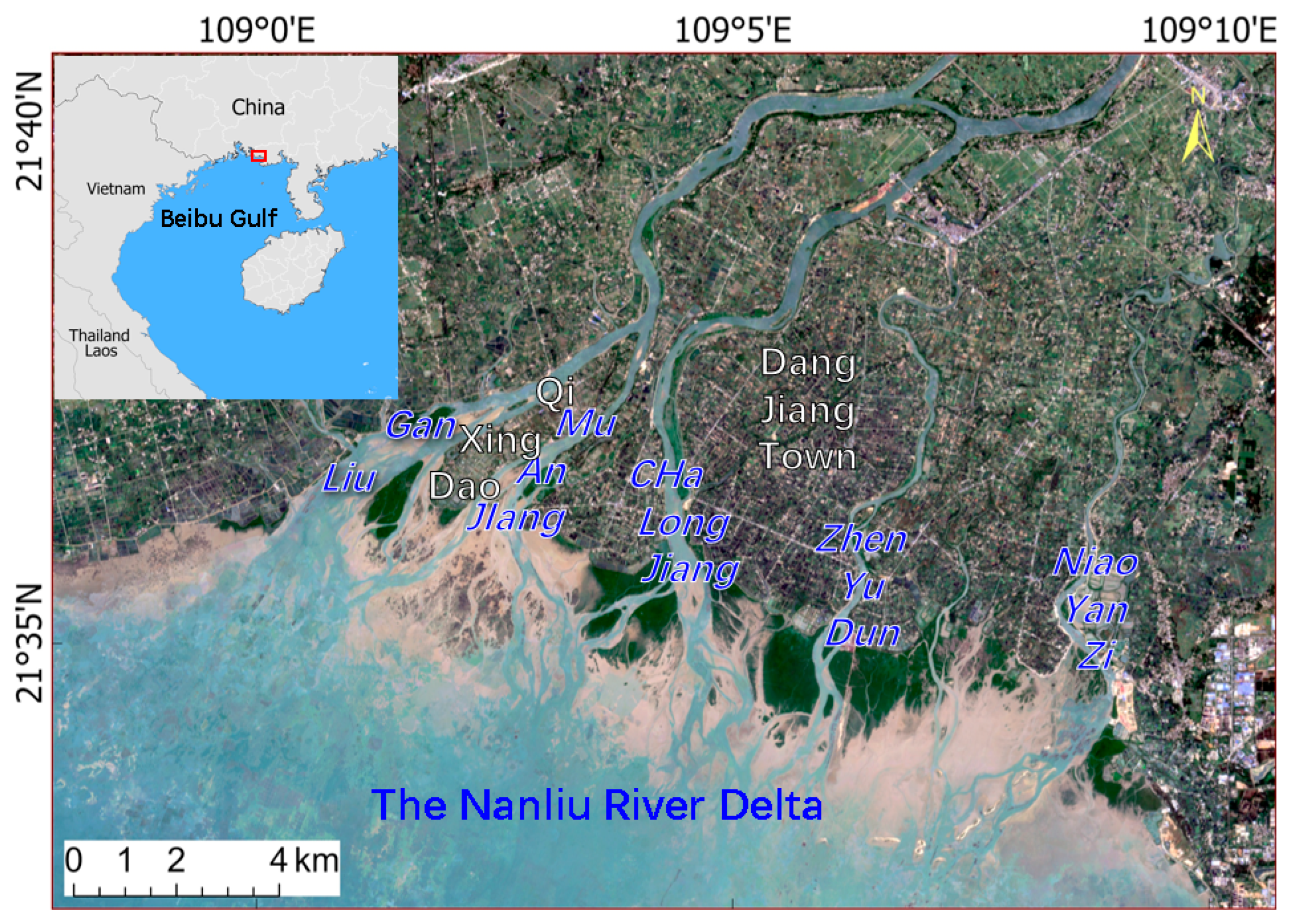
The Nanliu River Delta, the largest delta in the northern Beibu Gulf, is located in the Guangxi Zhuang Autonomous Region, southern China (approximately 21°30′–21°40′ N, 108°55′–109°10′ E), and discharges into the sea through five distributary channels (Figure 1). It is the largest independent river system flowing directly into the sea in Guangxi Province. The region lies within a northern tropical monsoon climate zone, characterized by hot, humid summers and mild, relatively dry winters.

The deltaic geomorphology is jointly controlled by fluvial sediment supply and tidal processes, forming extensive intertidal mudflats, dendritic tidal creeks, and gently sloping coastal depositional environments. According to long-term tidal gauge records from the Beibu Gulf coastal stations, the estuary experiences an irregular diurnal tidal regime with a mean tidal range of approximately 2.5 m, with strong tidal currents and frequent exposure–inundation cycles typical of intertidal mangrove habitats.

Mangrove vegetation on the tidal flats is dominated by Aegiceras corniculatum, Kandelia obovata, Avicennia marina, and Sonneratia apetala, while the main herbaceous species consist of Spartina alterniflora and Cyperus malaccensis. The Nanliu River Delta exhibits a distinct landward-to-seaward gradient of decreasing stand age. The intense interaction between fluvial runoff and extreme tidal ranges results in a complex, overlapping species distribution rather than strict zonation. Notably, mangrove degradation in this region is primarily characterized by structural and functional decline, with no evidence of species-specific successional replacement at present.

Building upon a legacy of mid-20th-century coastal development, the Nanliu River Delta has experienced intensive and observable human disturbances, including large-scale land reclamation, seawall construction, and rapid expansion of aquaculture ponds, which substantially altered shoreline morphology and hydrodynamic conditions. After 2000, national wetland conservation policies and mangrove restoration programs were gradually implemented, including plantation and rehabilitation projects in abandoned aquaculture areas and degraded tidal flats. These interventions have contributed to the recent increase in mangrove area but have also introduced new structural and ecological challenges, particularly related to forest aging, species invasion, and internal degradation.

Owing to its long-term interaction between natural tidal dynamics and successive phases of human disturbance and restoration, the Nanliu River Delta provides an ideal setting for investigating both mangrove extent change and degradation processes over multi-decadal timescales.

2.2. Remote Sensing Imagery and Auxiliary Data

2.2.1. Remote Sensing Imagery

To ensure temporal consistency and reproducibility, this study employed U.S. Geological Survey (USGS; Reston, VA, USA) Landsat Collection 2 Tier 1 Level-2 Surface Reflectance (SR) products from 1990 to 2025 using the Google Earth Engine (GEE; Google Inc., Mountain View, CA, USA) platform [45]. Specifically, we used Landsat 5 TM (LT05/C02/T1_L2), Landsat 7 ETM+ (LE07/C02/T1_L2), Landsat 8 OLI (LC08/C02/T1_L2) and Landsat 9 OLI-2 (LC09/C02/T1_L2). For each target epoch (1990, 1995, 2000, 2005, 2010, 2015, 2020, and 2025), we used a ±6 months temporal window to ensure sufficient valid observations for compositing.

All products provide atmospherically corrected surface reflectance and include the QA_PIXEL band for pixel-level quality control. Cloud, cloud shadow, cirrus, and snow pixels were removed using the QA_PIXEL bitmask according to the USGS Landsat Collection 2 specification. Specifically, pixels flagged as Cloud (bit 3), Cloud shadow (bit 4), Cirrus (bit 2), and Snow (bit 5) were masked out. In addition, a cloud-score-based threshold was applied to remove residual haze-contaminated pixels [46]. This two-step procedure is designed to facilitate reproducibility and reduce potential atmospheric contamination within the time series.

After May 2003, Landsat-7 ETM+ data are affected by the SLC-off issue. In this study, all SLC-off gap pixels were treated as no-data and excluded from compositing. No spatial interpolation was applied. Instead, NDVI-PP75 composites were constructed using valid pixels from overlapping scenes within each temporal window, which mitigates data loss and maintains statistical robustness.

All Landsat Collection 2 Level-2 SR products benefit from unified atmospheric correction, radiometric calibration, and geometric precision, providing a harmonized long-term surface reflectance record across Landsat 5/7/8/9. As a result, NDVI and EVI derived from these products are internally consistent and suitable for decadal-scale ecological monitoring [34,47].

2.2.2. Auxiliary Data

To enhance topographic adaptability in the automated extraction of intertidal mangroves, we incorporated a digital elevation model (DEM). Currently available global DEMs at 30 m resolution include Copernicus DEM GLO-30 [48], ALOS World 3D-30 m (AW3D30), ASTER GDEM, and SRTM30 DEM [49]. Among these, Copernicus DEM GLO-30 is derived from the TanDEM-X interferometric mission’s WorldDEM dataset, and has undergone specific optimizations for rivers, coastlines, and water bodies [50]. It provides improved performance in intertidal environments and shows higher detail and consistency in the transition zones between tidal flats and mangroves. Therefore, this study selected Copernicus DEM GLO-30 as the topographic auxiliary layer for elevation constraints.

2.3. Data Preprocessing

All preprocessing procedures were conducted in the GEE environment, including:

(1)

Filtering candidate images with cloud cover less than 30% to ensure high-quality observations.

(2)

Removing cloud and shadow pixels using the QA_PIXEL bitmask.

(3)

Extracting six spectral bands shared across all Landsat sensors—blue, green, red, near-infrared (NIR), shortwave infrared 1 (SWIR1), and shortwave infrared 2 (SWIR2)—to maintain spectral consistency.

(4)

Grouping images into eight target years (1990, 1995, 2000, 2005, 2010, 2015, 2020, 2025), using a ±6-month temporal window to ensure sufficient sample size.

(5)

Clipping all imagery to the extent of the Nanliu River Delta.

2.4. Low-Tide Image Compositing

Mangroves generally exhibit higher NDVI values than bare tidal flats and open water when exposed, whereas NDVI decreases markedly under tidal inundation. Therefore, NDVI can be used as an indicator of the surface exposure state in intertidal environments. Techniques such as NDVI Maximum Value Compositing (MVC) [27], median compositing [51], and various percentile-based approaches (e.g., 70th, 80th, or 90th percentiles) [24,26] have been widely utilized in existing literature to reconstruct cloud-free and low-tide surface reflectance in tidal wetlands.

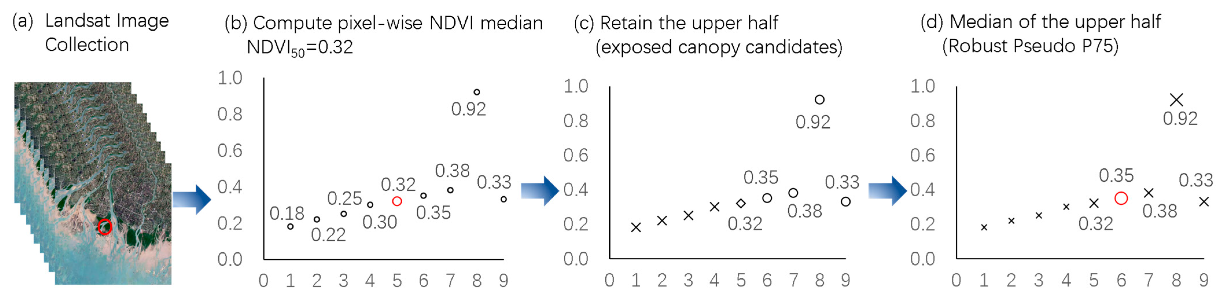
In this study, we propose an NDVI Pseudo-P75 Compositing method based on a Median-of-the-Upper-Half (MUH) strategy, designed to extract high-quality observations from multi-temporal Landsat stacks (Figure 2).

For each pixel location $x$ and time window $T$, the proposed algorithm is structured as follows:

Compute NDVI for each image $i\in T$:

$${NDVI}_i(x)={\displaystyle \frac{NIR\left(x\right)-RED\left(x\right)}{NIR\left(x\right)+RED\left(x\right)}}$$

(1)

Compute the pixel-wise median:

$${NDVI}_{50}\left(x\right)=median\left\{{NDVI}_i\left(x\right) \right|i\in T\}$$

(2)

Select the subset of high-quality observations:

$$S\left(x\right)=\left\{i\in T \right|{NDVI}_i\left(x\right)\ge {NDVI}_{50}\left(x\right)\}$$

(3)

Compute the filtered median composite:

$${NDVI}_{P75}\left(x\right)=median\{i\in S\left(x\right)\}$$

(4)

For numerical stability in floating-point computations, Equation (3) should be reformulated as:

$$S\left(x\right)=\left\{i\in T \right|{NDVI}_i\left(x\right)\ge {NDVI}_{50}\left(x\right)-\epsilon \}$$

(5)

where ε ∈ [10⁻⁴, 10⁻²] is a small numerical tolerance introduced to ensure robust floating-point comparisons. Sensitivity tests indicated that variations of ε within this range have no material impact on the composite.

This dual-median approach offers advantages in lower-tail suppression, outlier resilience, ecological representativeness, and computational scalability:

First-pass Median Filtering: The initial median reduction serves as a conservative filter to eliminate transient low-NDVI artifacts. In coastal environments, this effectively masks pixels contaminated by sub-optimal tidal states (inundation) and cloud shadows, ensuring that only the relatively vigorous spectral states are passed to the next stage.

Secondary Outlier Resistance: By applying a second median operation on the upper-half distribution, the MUH strategy filters out upper-tail anomalies, such as sensor saturation or sun glint.

Representative Ecological Centrality: Statistically, the median possesses strong “central tendency.” Our MUH logic can be framed as “selecting the most representative candidate from the most vigorous 50% of observations.” This approach mitigates the edge-case instability associated with extreme quantiles, allowing the composite to more closely represent the characteristic phenological state of the mangrove canopy.

Optimized Cloud-Computing Architecture: Within the Google Earth Engine (GEE) environment, ee.Reducer.median() is a highly optimized, native operator designed for massive parallelization. By nesting these native reducers, we bypass the computational overhead and “Time Out” risks associated with custom sorting or band-independent percentile calculations, thus ensuring full reproducibility and efficiency over our multi-decadal dataset. Although GEE offers native median and maximum compositors, it does not feature a standardized 75th percentile compositing function. Existing percentile reducers perform band-wise calculations, potentially leading to spectral misalignment.

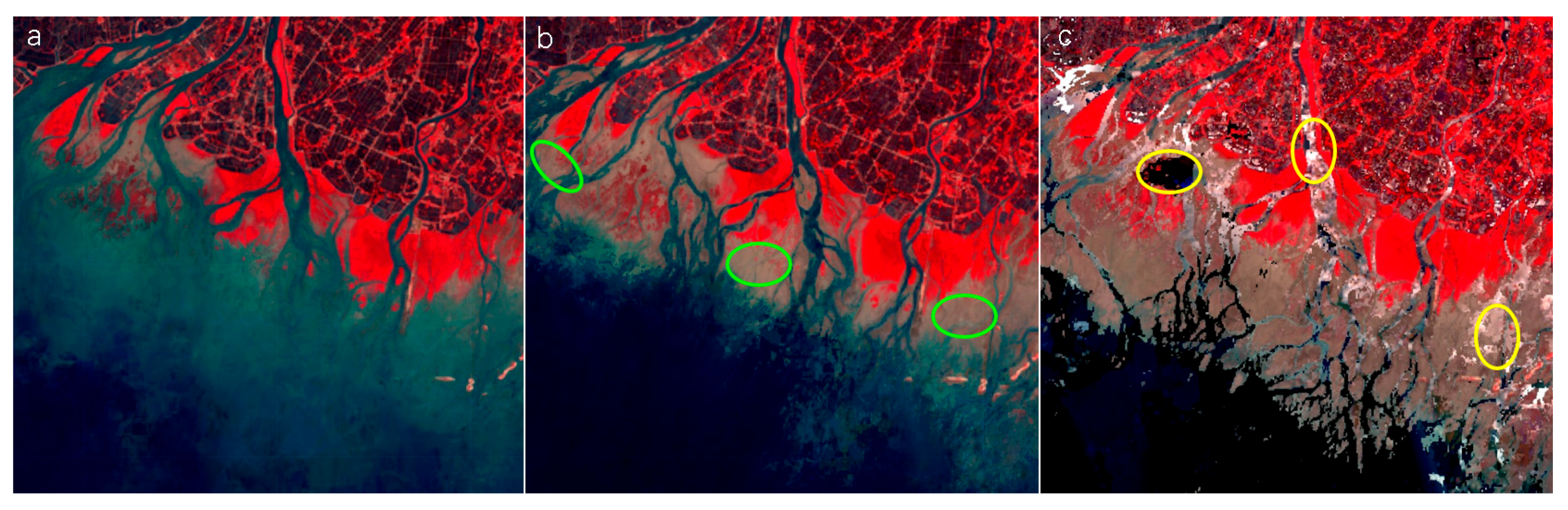
Compared with a standard median composite, NDVI-PP75 enhances the representation of exposed intertidal surfaces (Figure 3a,b). Compared with a maximum-value composite (MVC), it avoids instability caused by extreme NDVI outliers related to atmospheric scattering or sensor noise (Figure 3b,c).

The NDVI-PP75 composite is intended as a heuristic, exposure-biased observation selection strategy rather than a physical tide-level reconstruction.

Using this method on the GEE platform, NDVI-PP75 composites were generated for the target years 1990, 1995, 2000, 2005, 2010, 2015, 2020, and 2025.

2.5. Deep Learning Model

2.5.1. Training Labels and Independence

Training labels were derived from two high-quality global mangrove products for the reference year 2020: Global Mangrove Watch v4 (GMW v4) and the High-Resolution Global Mangrove Forest (HGMF2020). HGMF2020 was used within China due to its higher regional accuracy, while GMW v4 was adopted for other areas. Both datasets are based on Sentinel-2 imagery at 10 m spatial resolution and provide reliable, independent references for mangrove extent in 2020. Simultaneously, we performed a meticulous manual correction of the HGMF2020 dataset within study area, utilizing Google Earth high-resolution historical imagery and unmanned aerial vehicle (UAV) orthophotos as reference.

These products were used only to initialize training labels for the 2020 epoch. The ResNet34–UNet model was trained on Landsat Collection 2 Level-2 Surface Reflectance imagery using global labels and then applied consistently to other years (1990–2025), benefiting from the cross-sensor harmonization of the Landsat Collection 2 time series.

To avoid circular validation, the 2020 reference labels were not used to validate maps of other years. Moreover, the final mangrove maps for all epochs were subjected to independent verification and manual correction using high-resolution Google Earth imagery, UAV observations, and field survey sample points. This hybrid validation strategy helps decouple the model assessment from the 2020 reference datasets, thereby reducing the risk of circular validation and enhancing the reliability of the multi-temporal products.

By incorporating both Landsat-7 and Landsat-8 imagery into the training phase rather than relying on a single sensor, the model learns to extract sensor-invariant features, thereby effectively accommodating the radiometric differences between various instruments.

2.5.2. Control of Spatial Autocorrelation and Validation Strategy

Spatial autocorrelation can artificially inflate accuracy when training and testing samples are spatially adjacent. To mitigate this risk, our model training and evaluation did not rely on random pixel-level splits within the same local study area.

First, the network was pre-trained using the full-coverage global mangrove reference datasets, including the complete Global Mangrove Watch v4 (GMW v4) dataset [14] worldwide and HGMF2020 dataset [27] within China. Our comparative analysis revealed that while GMW v4 excels globally, HGMF2020 provides superior accuracy in China, particularly in the Nanliu River Delta. By integrating both, the model benefits from high-quality local labels while maintaining global context, thereby minimizing spatial dependency and enhancing the model’s generalization beyond any single estuary or region.

Second, the pre-trained model was transferred to the Nanliu River Delta and applied to multi-temporal Landsat imagery from 1990 to 2025. For each epoch, the extracted mangrove maps were independently verified and corrected using high-resolution Google Earth imagery, UAV observations, and field sample points, rather than using randomly sampled pixels from the same region for validation.

Therefore, the reported accuracy does not originate from spatially adjacent train/test samples within the Nanliu River Delta, and the risk of spatial autocorrelation-driven accuracy inflation is substantially reduced. Although a formal spatially blocked cross-validation was not implemented due to computational and data constraints, the combination of cross-region pretraining and independent high-resolution verification provides a robust and conservative assessment of model reliability at the estuary scale.

2.5.3. Model Training Configuration and Hyperparameters

Model training was implemented using the ArcGIS Pro (Esri, Redlands, CA, USA) deep learning framework. All accessible hyperparameters were explicitly specified to ensure reproducibility.

The input image chips were generated with a fixed patch size of 256 × 256 pixels, corresponding to 7.68 km × 7.68 km at 30 m Landsat resolution. The batch size was set to 16, and the model was trained for a maximum of 50 epochs. An early stopping strategy was employed to prevent overfitting by terminating training when validation performance no longer improved.

The optimizer employed by the ArcGIS Pro (v3.5) is based on the Adam algorithm. The learning rate was automatically tuned within a range of 5.2481 × 10⁻⁶ to 5.2481 × 10⁻⁵, and the optimal value was selected from the learning curve during training [52].

Class balancing (weighted sampling) was applied during data loading to ensure that mangrove samples were adequately represented in each batch. The loss function combined Dice Loss and Cross-Entropy Loss to enhance segmentation performance: Dice Loss improves class overlap sensitivity and is effective for small-object segmentation, while Cross-Entropy facilitates accurate pixel-level discrimination. Focal Loss [53] was further integrated to reduce the dominance of easily classified background samples on gradient updates.

Data augmentation was applied to improve generalization and reduce overfitting, including:

(1)

random rotation within ±30° with a probability of 0.5;

(2)

random brightness adjustment in the range 0.4–0.6;

(3)

random contrast adjustment in the range 0.75–1.5;

(4)

random zooming with a scale factor between 1.0 and 1.2;

(5)

random cropping, with crop positions uniformly sampled across the chip.

All other hyperparameters and configurations were maintained at the default values provided by the ArcGIS Pro (v3.5) Deep Learning Toolbox.

2.5.4. Classification Accuracy and Robust Performance Metrics

Model training followed a two-stage strategy. First, the encoder (backbone) was frozen and only the decoder was trained to achieve stable feature learning. Training was stopped when performance on an independent validation set ceased to improve. Then, all layers were unfrozen and the entire network was fine-tuned with early stopping until validation accuracy converged.

To provide a rigorous evaluation of segmentation performance, we report a confusion matrix and class-wise Precision, Recall, F1-score, and Intersection over Union (IoU) for both mangrove and non-mangrove classes (

Table 1. ResNet-34-UNet model metrics training with DEM.

Metrics	Precision	Recall	F1-Score	IoU
background	0.990	0.992	0.992	0.981
mangrove	0.910	0.895	0.902	0.822

).

Overall accuracy was 98.17%, while mean IoU (mIoU) across both classes was 0.902 and was computed as the arithmetic mean of class-wise IoU values for mangrove and background classes.

For the mangrove class, the model achieved a Precision of 0.910, Recall of 0.895, and F1-score of 0.902, corresponding to an IoU of 0.822. For the background class, Precision, Recall, and F1-score reached 0.990, 0.992, and 0.992, respectively, with an IoU of 0.981. The mean IoU (mIoU) across both classes is 0.902.

These results demonstrate that the ResNet34–UNet framework achieves high discrimination ability not only for the dominant background class but also for the mangrove class, which is more challenging due to spectral similarity with tidal flats and salt-marsh vegetation.

2.5.5. Baseline Model Comparison and Architecture Selection

To justify the incremental value of the proposed pipeline, we conducted a systematic comparison across multiple encoder–decoder architectures, backbone networks, and auxiliary data configurations. Specifically, we evaluated four representative semantic segmentation frameworks: U-Net [42], Pyramid Scene Parsing Network (PSPNet), DeepLabV3, and SAM-LoRA. For backbone encoders, we tested ResNet-18, ResNet-34 [41], Xception, EfficientNet-B0, and CaresNet50T.

In addition, each architecture was trained under two configurations: (i) using multispectral bands and NDVI only, and (ii) integrating DEM as an auxiliary geomorphological constraint. The results show that U-Net consistently outperformed PSPNet, DeepLabV3, and SAM-LoRA.

The integration of DEM significantly refines the classification by capturing micro-topographic variations critical to intertidal distribution. Quantitative verification indicates that including elevation data improves the mangrove extraction accuracy by 1.9% in F1-score (Table 1 and

Table 2. ResNet-34-UNet model metrics training without DEM.

Metrics	Precision	Recall	F1-Score
background	0.988	0.991	0.989
mangrove	0.896	0.871	0.883

).

Among the tested backbones, ResNet-34 and CaresNet50T ranked as the top two performers. Although CaresNet50T achieved slightly higher IoU (+0.18 on average), its computational cost was substantially higher: training required more than one week of continuous runtime, compared with approximately two days for ResNet-34. This high computational burden increased the risk of interrupted training and reduced practical feasibility for large-scale and multi-temporal mapping.

Considering both accuracy and computational efficiency, the U-Net + ResNet-34 + DEM configuration was selected as the final model for this study.

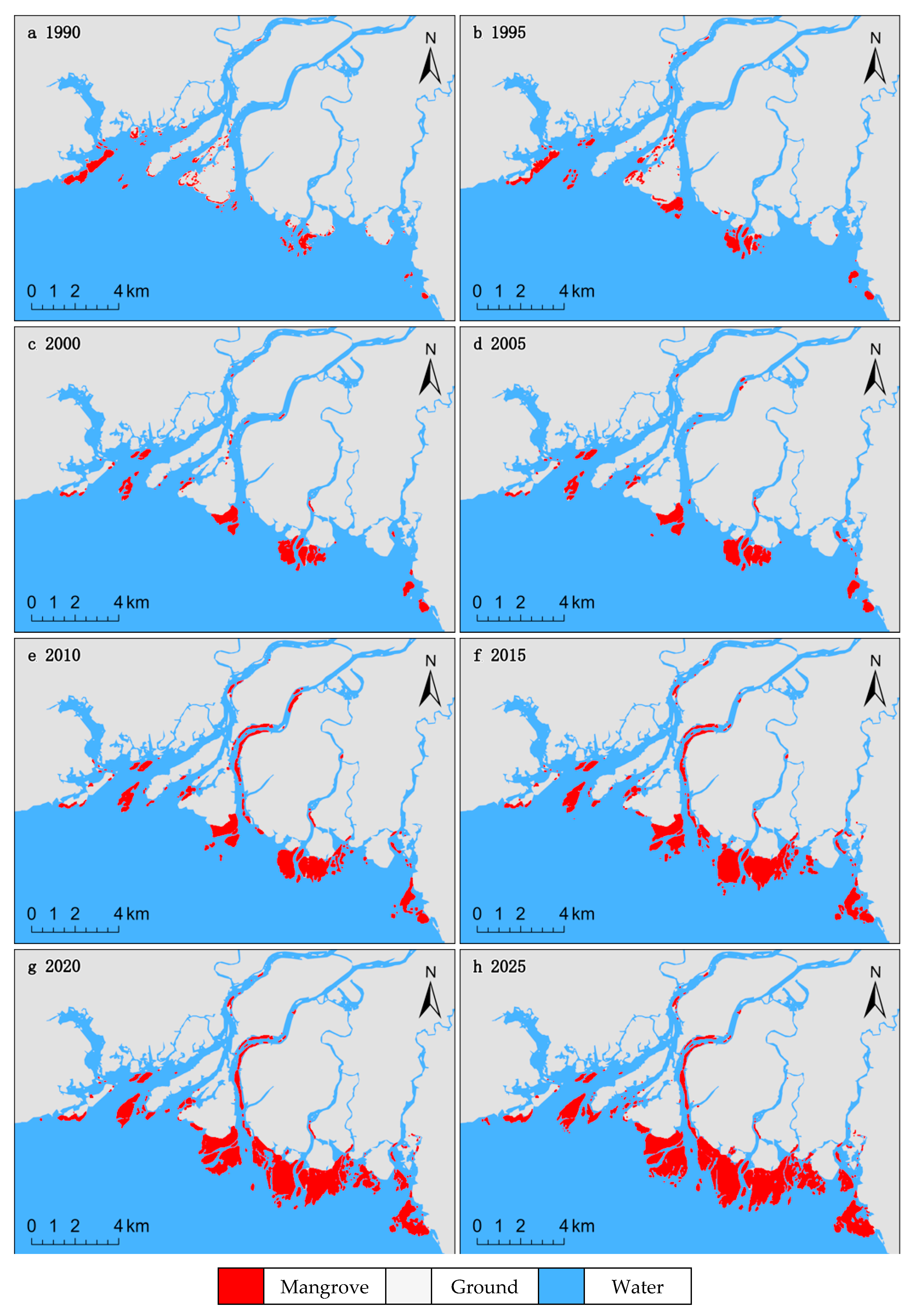
After training, the model was applied to low-tide composites for each target year from 1990 to 2025 to produce eight epochs of mangrove distribution maps (Figure 4).

2.6. Change Detection and Definitions

To ensure geometric consistency and accurate area calculations, all spatial datasets were projected into the local UTM Zone 49 coordinate system. Mangrove change was quantified by overlay analysis between consecutive mangrove maps at each target epoch.

We define the change categories as follows:

Loss: A pixel (or polygon) classified as mangrove at time $t_i$ but not classified as mangrove at time $t_{i+1}$.

$$Los{s}_i=M\left(t_i\right)\cap \neg M\left(t_{i+1}\right)$$

(6)

Gain: A pixel classified as non-mangrove at time $t_i$ but classified as mangrove at time $t_{i+1}$.

$$Gai{n}_i=\neg M\left(t_i\right)\cap M\left(t_{i+1}\right)$$

(7)

where $M\left(t\right)$ denotes the mangrove map at time $t$.

Cumulative Loss: The spatial union of all loss patches across the full study period:

$$Cummulative Loss = \bigcup _{i=1}^{n-1}{Loss}_i$$

(8)

This metric captures the total footprint of areas that experienced mangrove disappearance at least once during 1990–2025.

Recovery (Descriptive): we did not compute a formal recovery index, recovery is used descriptively to refer to pixels that experienced a loss at an earlier time and were later reclassified as mangrove (i.e., loss → gain cycles).

2.7. Area Calculation

All raster change maps were converted into vector format and reprojected to UTM Zone 49. Polygon areas were automatically calculated in ArcGIS using planar geometry, ensuring accurate area estimation in hectares.

Because the study area includes a rectangular buffer enclosing the entire Nanliu River Delta (not limited only to exposed tidal flats), shoreline position and tidal flat migration do not affect the consistency of mangrove area statistics across periods.

2.8. Mangrove Health Assessment

Vegetation indices (VIs) derived from multispectral reflectance provide effective proxies for canopy structure, chlorophyll content, and photosynthetic activity, and are widely used for assessing vegetation condition and health [54,55]. Among these indices, the Normalized Difference Vegetation Index (NDVI) and Enhanced Vegetation Index (EVI) are the two most widely used metrics in remote sensing studies [56,57,58].

NDVI is calculated from red and near-infrared (NIR) reflectance but saturates in dense vegetation. When leaf area index (LAI) exceeds a threshold, NDVI becomes less sensitive to vegetation changes [59,60]. NDVI is also susceptible to atmospheric scattering, aerosols, and soil background, which can lead to systematic underestimation in wet, highly reflective environments such as mangrove forests [61].

The EVI was developed to address NDVI’s limitations. It incorporates the blue band for atmospheric correction and employs a soil adjustment factor to reduce background and aerosol interference, providing a more accurate representation of canopy optical properties and photosynthetic activity [62,63]. Studies have demonstrated that EVI is more sensitive to canopy structure and leaf nitrogen content in high-biomass ecosystems such as mangroves and tropical rainforests, enabling better differentiation of vegetation health conditions [57,64]. Therefore, EVI was selected as the primary index for mangrove health assessment in this study.

The EVI is calculated as:

$$EVI=2.5\times {\displaystyle \frac{(NIR-RED)}{(NIR+6\times RED-7.5\times BLUE+1)}}$$

(9)

where NIR, RED, and BLUE represent surface reflectance values (0–1). The coefficient 2.5 is a gain factor; L = 1 is the canopy background adjustment term; and C₁ = 6 and C₂ = 7.5 are aerosol correction coefficients [56,57]. EVI values typically range from −1 to +1, with higher values indicating greater vigor, higher biomass, and better vegetation health.

In this study, mangrove degradation is defined as a spectral proxy assessment based on ΔEVI, reflecting a relative decline in canopy vigor. It should be noted that this remote-sensing-based approach focuses on the physiological and structural changes of the canopy and does not encompass a full-spectrum ecological diagnosis, which would typically require in situ data on biodiversity and soil health.

Mangrove canopy condition and internal degradation were assessed using inter-period changes in the Enhanced Vegetation Index (ΔEVI). For each pixel classified as mangrove at both time $t_i$ and $t_{i+1}$, ΔEVI was calculated as:

$$\Delta EVI=EVI\left(t_{i+1}\right)-EVI\left(t_i\right)$$

(10)

Only pixels continuously classified as mangrove in both epochs were included in the quality analysis. Pixels identified as “loss” (mangrove → non-mangrove) were excluded from ΔEVI-based degradation assessment to avoid conflating canopy decline with complete habitat disappearance.

The ΔEVI classification thresholds were defined based on a combination of (i) literature benchmarks and (ii) empirical interpretation using high-resolution reference data. Previous studies in forest and vegetation time-series analysis have shown that significant negative shifts in EVI often correspond to disturbance or stress events, whereas near-zero changes typically reflect stable canopy conditions [65]. Additionally, long-term vegetation index time-series analyses emphasize that change detection thresholds should be informed by statistical behavior of the index over time rather than arbitrary cut-offs [66].

To determine appropriate thresholds for EVI change classification, we first summarized the statistical properties of EVI values across eight representative study periods (

Table 3. EVI statistical values for representative years.

Year	Mean	STD DEV
1990	0.27	0.10
1995	0.22	0.11
2000	0.29	0.09
2005	0.30	0.10
2010	0.34	0.10
2015	0.35	0.12
2020	0.37	0.12
2025	0.37	0.11

). As shown, the standard deviation of EVI is consistently close to 0.09–0.12 in all years, indicating a relatively stable background variability.

In many remote sensing change-detection studies, values within approximately ±1 standard deviation (σ) are commonly interpreted as reflecting “normal” or “stable” fluctuations, whereas deviations beyond ±σ indicate noticeable change, and those exceeding ±2σ are often regarded as significant change. Based on this empirical principle, we used σ ≈ 0.10 as a reference scale to define the ΔEVI classification thresholds.

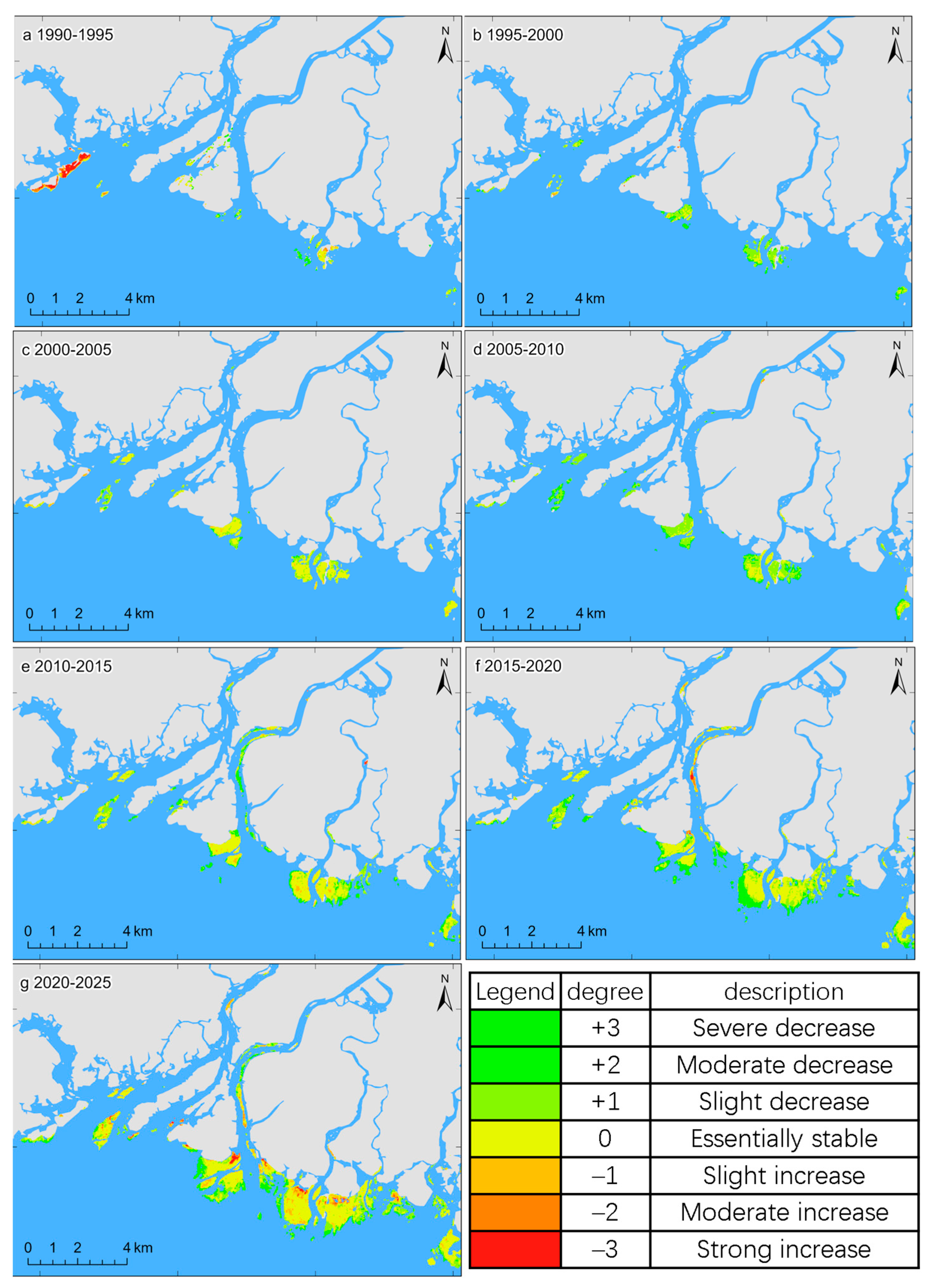
To further capture more subtle vegetation dynamics, we subdivided the ΔEVI range into seven ordinal levels using ±0.5σ intervals (

Table 4. Classification of EVI change levels.

Level	Description	ΔEVI Range Baseline	ΔEVI Range Conservative (+20%)	ΔEVI Range Relaxed (−20%)
−3	Severe decrease	−1.00~−0.25	−1.00~−0.30	−1.00~−0.20
−2	Moderate decrease	−0.25~−0.15	−0.30~−0.18	−0.20~−0.12
−1	Slight decrease	−0.15~−0.05	−0.18~−0.06	−0.12~−0.04
0	Essentially stable	−0.05~+0.05	−0.06~+0.06	−0.04~+0.04
1	Slight increase	+0.05~+0.15	+0.06~+0.18	+0.04~+0.12
2	Moderate increase	+0.15~+0.25	+0.18~+0.30	+0.12~+0.20
3	Strong increase	+0.25~+1.00	+0.30~+1.00	+0.20~+1.00

), representing severe, moderate, and slight decrease, stable, and slight, moderate, and strong increase, respectively.

To calibrate the breakpoints, we visually compared ΔEVI patterns with independent high-resolution evidence, including Google Earth imagery, UAV orthophotos, and field observations (2020–2025). The threshold of 0.05 was selected to distinguish meaningful ecological changes from background noise. In mangrove ecosystems, minor EVI fluctuations (typically |ΔEVI| < 0.05) are often attributed to phenological seasonality, short-term meteorological disturbances (e.g., wind and precipitation), and residual sensor noise. By defining |ΔEVI| ≤ 0.05 as ‘Essentially Stable’ category, we ensure that the identified degradation (starting from −0.05 to −0.15) represents observable physiological stress or canopy thinning rather than random environmental variations.

To assess the robustness of our degradation assessment and address potential uncertainties in threshold selection, we conducted a sensitivity analysis by perturbing the baseline ΔEVI thresholds. Two alternative scenarios were established by scaling the baseline thresholds (T) by ±20%: a Relaxed Scenario (0.8 × T) and a Conservative Scenario (1.2 × T). The Relaxed Scenario employs narrower intervals for the ‘Stable’ class, making the detection of slight degradation or recovery more sensitive, whereas the Conservative Scenario requires larger spectral shifts to trigger a class change (Table 4).

Mangrove “loss” and “quality decline” were treated as mutually exclusive categories. Pixels classified as loss (mangrove → non-mangrove) were not included in ΔEVI calculations. Quality decline refers only to internal canopy degradation within areas that remain classified as mangrove. Therefore, no overlap exists between loss and degradation categories in this study.

3. Results

3.1. Spatiotemporal Dynamics and Trends of Mangroves

3.1.1. Changes in Mangrove Area

Based on the mapped mangrove distributions (Figure 4), mangrove areas were quantified for representative years (Figure 5). To characterize the non-linear dynamics of mangrove trajectories, we utilized piecewise linear regression across distinct periods. This segmented approach confirms that mangrove expansion underwent significant rate changes around 2005. In 1990, the mangrove area in the Nanliu River Delta was 266 ha. By 2005, mangrove coverage increased to 379 ha, indicating a slow expansion during this period. Linear regression analysis shows an average annual increase of 7.61 ha yr⁻¹. By 2025, the mangrove area had expanded substantially to 1414 ha. According to the linear fit for the period 2005–2025, the average annual increase reached 51.96 ha yr⁻¹, which is approximately 6.8 times higher than that observed during the earlier period.

As summarized in

Table 5. Summary of mangrove area and net change rates in the Nanliu River Delta (1990–2025).

Period/yr	Start Area (ha)	End Area (ha)	Net Change (ha)	Annual Rate (ha/yr)	Major Trend
1990–2005	266	379	113	7.53	Slow Net Change under Active Land Conversion
2005–2015	379	859	480	48.00	Slow Recovery
2015–2025	859	1414	555	55.50	Rapid Expansion

, the mangrove ecosystem underwent a three-stage evolutionary process. The first period (1990–2005) was characterized by Slow Net Change under Active Land Conversion, with a relatively modest annual expansion rate of 7.53 ha/yr. This was followed by a Slow Recovery phase (2005–2015), where the growth rate surged to 48.00 ha/yr. Most notably, the last decade (2015–2025) witnessed Rapid Expansion (55.50 ha/yr), reflecting the significant impact of recent large-scale restoration initiatives.

3.1.2. Spatial Dynamics of Mangrove Distribution

The spatial distribution of mangroves in the Nanliu River Delta exhibits typical characteristics of estuarine wetlands (Figure 4). Mangroves are predominantly concentrated on silty tidal flats along both sides of the river mouth, forming sinuous “fringe belts” that run approximately parallel to the coastline. Their distribution is closely associated with the complex tidal creek network of the estuary, with mangroves extending landward along tidal channels. However, establishment is limited in zones with strong bidirectional tidal currents, such as deep channels within the main river course. The most extensive and continuous mangrove stands occur in the central–southern part of the estuary, where fluvial and marine hydrodynamic forces converge and sediment deposition is most pronounced, creating optimal habitat conditions for mangrove growth.

From 1990 to 2025, mangrove distribution in the Nanliu River Delta transitioned from an initially fragmented pattern to a phase of rapid expansion. Between 1990 (Figure 4a) and 1995 (Figure 4b), mangroves were sparsely distributed and primarily consisted of small, isolated patches along marginal zones. By 2000 (Figure 4c), total mangrove area remained relatively stable, although localized losses and increased fragmentation were evident. A notable shift occurred by 2005 (Figure 4d), when mangrove patches in core aggregation zones—particularly in the central–southern estuary—began expanding seaward and into adjacent vacant areas, resulting in a gradual increase in total area.

By 2010 (Figure 4e), expansion intensified, with a clear increase in mangrove extent relative to 2000, and previously fragmented patches started to coalesce into larger contiguous areas, mainly in depositional zones along the outer estuary. During 2015 (Figure 4f) and 2020 (Figure 4g), mangrove expansion entered an accelerated phase, characterized by the near-complete connection of formerly discrete patches into extensive continuous mangrove belts. Along both sides of the main river channel, mangroves also expanded landward into the interior of tidal creek networks, resulting in a substantial enlargement of their spatial extent. By 2025 (Figure 4h), the overall expansion trend persisted, and the primary distribution areas formed relatively continuous ecological communities, although localized canopy gaps remained in some sections.

Overall, before 2000, mangroves in the Nanliu River Delta were characterized by localized loss and fragmentation, with the total area remaining relatively stable or exhibiting only marginal growth. However, from 2005 to 2025, the system transitioned into a phase of sustained and rapid net expansion, primarily colonizing sediment-rich tidal flats and estuarine depositional zones. Across the entire 35-year study period, this growth was predominantly characterized by a distinct seaward expansion

3.2. Mangrove Area Loss

3.2.1. Quantitative Characteristics of Mangrove Area Loss

Mangrove area loss dynamics were quantified through difference analysis between consecutive temporal mangrove maps (Figure 4), and the results are summarized in Figure 6. During the study period, a total mangrove loss of 347.45 ha was recorded in the Nanliu River Delta. The period from 1990 to 1995 experienced the most severe mangrove loss, with a total loss of 134 ha, corresponding to an average annual loss rate of 26.8 ha yr⁻¹. This indicates that mangroves were subjected to intense disturbance during this stage.

Between 1995 and 2000, mangrove loss declined to 67 ha, approximately half of that observed in the previous period, suggesting a relative reduction in external pressures. From 2000 to 2010, mangrove loss reached a minimum, with losses of only 11 ha and 6 ha during the 2000–2005 and 2005–2010 intervals, respectively. During 2010–2015, mangrove loss increased again to 36 ha, implying that parts of the mangrove ecosystem were affected by rising environmental stress or natural degradation processes. In the subsequent period from 2015 to 2025, mangrove losses reached 52 ha and 42 ha, respectively, indicating that mangroves in the study area continued to face substantial threats during this period.

Notably, the decade from 1990 to 2000 represented the most acute phase of mangrove depletion, with a cumulative loss of 200.93 ha, accounting for 57.83% of the total loss observed across the entire 35-year study period.

3.2.2. Spatial Distribution and Patterns of Mangrove Loss

• Spatial Extent of Mangrove Loss

Mangrove loss maps for different periods (Figure 7) reveal clear stage-dependent dominant mechanisms. During 1990–2000 (Figure 7a,b), loss patches were large and spatially concentrated, occurring primarily along seawalls, reclaimed agricultural areas, and the peripheries of early aquaculture ponds. In 2000–2010 (Figure 7c,d), the size of loss patches decreased markedly, exhibiting a scattered and isolated pattern, indicating a relatively stable phase for estuarine mangroves. In 2010–2025 (Figure 7e–g), loss patches increasingly appeared within mangrove interiors or inside peninsular extensions, showing a characteristic “gap-forming” (canopy-opening) degradation pattern.

The cumulative loss map (Figure 7h) indicates that, after 35 years of aggregation, affected areas formed a continuous alongshore belt, constituting a distinct “landward loss belt.” The spatial footprint of cumulative loss totals 337 ha, which is 10 ha less than the cumulative loss area, accounting for approximately 2.9% of the total cumulative loss. This discrepancy indicates that about 10 ha of mangrove patches experienced repeated cycles of loss, recovery, and subsequent loss.

In the Nanliu River Delta, mangrove dynamics are dominated by a spatially asymmetric pattern: persistent seaward expansion at the tidal-flat front and early-stage landward encroachment by aquaculture and seawall construction (Figure 4 and Figure 7). As a result, large areas of mangroves were permanently converted in the 1990s, whereas later decades show much smaller landward losses and mainly internal degradation.

Therefore, the cumulative loss (the spatial union of all loss events from 1990–2025) reflects the historical footprint of human encroachment, not a reversible cycling process. Overlay analysis between the cumulative loss map and the 2025 mangrove distribution shows that only 30 ha of previously lost areas have been re-occupied by mangroves, whereas 307 ha remain unrecovered, indicating that most loss is permanent rather than cyclical.

By integrating the five distributary channels at the Nanliu River mouth (Figure 1) with period-specific loss maps (Figure 7), pronounced spatial heterogeneity in mangrove loss is evident. During 1990–1995, losses were concentrated along the main channel, the Muanjiang River, and the banks of the Chalong River and Zhenyudun. In 1995–2000, large-scale losses persisted along the western side of the main channel. During 2000–2005, losses were mainly confined to the Chalong River. From 2005–2010, mangrove loss declined to its minimum and appeared only sporadically. In 2010–2015, loss expanded toward the main channel and upstream sections of the Chalong River. During 2015–2020, losses again concentrated along the Chalong River. In 2020–2025, loss patches were more frequently distributed along the landward margins of mangrove stands.

From the cumulative loss pattern for 1990–2025, mangrove losses were primarily concentrated along riverbanks and the inner (landward) side of tidal flats. In contrast, the seaward mangrove fronts exhibited no extensive, continuous loss patches, showing only sporadic occurrences.

• Influence of Distance to Seawalls on Mangrove Loss

In this study, seawalls are used as a comprehensive proxy for anthropogenic boundaries. Given the rural and aquaculture-dominated landscape of the Nanliu River Delta, these structures are typically co-located with coastal roads and aquaculture pond embankments, forming a definitive hardened boundary between land and sea. Consequently, the seawall buffers effectively encapsulate the primary anthropogenic gradients, including transportation and land-reclamation pressures.

Seawall locations were manually digitized using high-resolution Google Earth imagery acquired in November 2021. The imagery has a spatial resolution finer than 1 m, allowing clear visual identification of seawall crests and revetment structures. Digitization was conducted at a scale of 1:1000–1:2000 to ensure geometric precision. Thirty buffer zones were generated at 50 m intervals within a 50–1500 m range to quantify mangrove loss within each buffer (Figure 8a). Results show that 103 ha of mangrove loss occurred within 50 m of existing seawalls, accounting for 30.6% of the total loss. Losses of 85.4 ha, 57.6 ha, and 32.6 ha were observed within the 50–100 m, 100–150 m, and 150–200 m zones, respectively.

Overall, mangrove loss within 200 m of seawalls reached 278.6 ha, representing 82.7% of the total loss. Loss area decreased rapidly with increasing distance from seawalls, exhibiting a pronounced inverse J-shaped distribution.

To quantify the impact of seawall proximity on mangrove vulnerability, we calculated the Cumulative Distribution Function (CDF) based on all mangrove loss pixels. The results demonstrate a sharp spatial clustering: 84.9% of the mangrove loss occurred within 200 m of the nearest seawall (Figure 8b). This concentration suggests that seawall infrastructure acts as a critical driver of localized mangrove degradation and loss.

Given the sub-meter resolution of the source imagery, the positional uncertainty of the digitized seawall lines is estimated to be within ±1–2 m, which is small relative to the 50 m buffer interval used in the proximity analysis. Therefore, digitizing error is unlikely to materially affect the observed inverse J-shaped relationship between mangrove loss/degradation and distance to seawalls.

Although seawalls were digitized from 2021 imagery, they represent long-standing, permanent human infrastructure. Their spatial distribution captures the cumulative footprint of coastal engineering and reclamation activities and is appropriate for analyzing the historical spatial constraint on mangrove dynamics.

• Developmental Patterns of Mangrove Loss

The spatial evolution of mangrove loss in the Nanliu River Delta can be summarized as follows: losses initially concentrated on the western side of the main channel, subsequently expanded to both the eastern and western sides of the island between the Muanjiang and Chalong rivers, and in later stages showed a tendency to extend toward the vicinity of Zhenyudun (Figure 9).

3.3. Mangrove Quality

3.3.1. Quantitative Characteristics of Mangrove Quality Decline

To characterize the health dynamics of mangroves in the Nanliu River Delta during 1990–2025, this study uses inter-period EVI differencing (ΔEVI) and predefined thresholds (Table 3) to classify mangrove quality changes into seven levels, ranging from severe ΔEVI decrease to strong increase. The area and magnitude of change for each class were calculated (Figure 10).

It should be noted that ΔEVI-based categories represent a remote-sensing proxy for canopy vigor change rather than a full ecological diagnosis. Therefore, the mapped areas of “degradation” should be interpreted as indicative patterns of relative decline, not as definitive assessments of ecosystem health at the physiological or species level.

During 1990–1995, ΔEVI indicates a high proportion of degraded pixels: severe decrease reached 29.07 ha, moderate decrease 14.58 ha, and slight decrease 18.18 ha, totaling 61.83 ha and accounting for 40.01% of the sampled pixel area for that period. In contrast, areas with improvement included 35.37 ha (slight), 14.22 ha (moderate), and only 1.71 ha (strong). Overall, decrease area exceeded restored area in this period.

From 1995–2000, decrease areas decreased markedly: severe decrease was only 0.54 ha, moderate decrease 1.08 ha, and slight decrease 3.60 ha, indicating a clear recovery trend. This period represents a key transition from a highly degraded phase to a recovery-dominated phase.

Between 2000–2005, moderate and severe decrease declined further to 0.18 ha and 0.09 ha, respectively, while slight decrease was 12.06 ha. In 2005–2010, slight decrease was 3.78 ha, moderate decrease 0.81 ha, and severe decrease was absent, suggesting further alleviation of stress on mangroves.

Changes became evident during 2010–2015: slight decrease increased substantially to 30.24 ha, while moderate and severe decrease were each 0.99 ha. These results indicate increasing internal growth heterogeneity, with some areas entering slight decrease. From 2015–2020, slight decrease remained high (26.10 ha), while moderate and severe decrease increased to 7.65 ha and 2.43 ha, respectively, implying the coexistence of recovery and degradation processes. During 2020–2025, ΔEVI exhibited pronounced changes: slight decrease surged to 103.05 ha, the highest among all periods, with moderate and severe decrease rising to 23.13 ha and 15.93 ha, respectively.

The maximum absolute difference was observed in the ‘Essentially stable’ category during 2020–2025, reaching 84.15 ha (7.73% of the total mangrove area in that period). The maximum relative difference occurred in the ‘Essentially stable’ category during 2000–2005, with a variance of 30.69 ha, accounting for 10.28% of the contemporaneous mangrove area. On average, the absolute area difference across all periods was 11.6 ha, with a mean relative difference (the ratio of the variance to the mangrove area in that period) of 2.4%. The trajectories of mangrove ΔEVI remained highly consistent across all threshold configurations (Figure 10), demonstrating the robustness of our assessment results.

Overall, from 1990–2025, mangrove ΔEVI in the Nanliu River Delta shows a clear stage-wise trajectory: pronounced early degradation → mid-term stabilization and rapid recovery → recent coexistence of recovery and degradation, with increasing areas of slight and moderate decrease after 2010.

3.3.2. Spatial Distribution of Quality Decline Patches

• Effect of Distance from the Coastline on Mangrove Quality Decline

Based on Google high-resolution imagery, seawalls were delineated, and 30 buffer zones were generated at 50 m intervals within a range of 50–1500 m to quantify mangrove quality decline within each buffer (Figure 11). The results also exhibit a clear inverted J-shaped distribution. Mangrove quality decline within 200 m of the seawall totals 159.67 ha, accounting for 58.0% of the total decrease area. Within 350 m of the seawall, the cumulative decrease area reaches 208.12 ha, representing approximately 75.6% of the total.

• Influence of Tributary Distribution on Mangrove Quality Decline

By integrating the five distributaries at the Nanliu River Delta with the spatial distribution of mangrove quality changes for each period (Figure 12), a pronounced spatial differentiation in mangrove quality degradation is observed. During 1990–1995, large-scale quality decline patches appeared on the western side of the main channel. From 1995–2010, no substantial large-scale degradation patches were evident. After 2010, distinct quality decline patches began to emerge within the interior of the mangrove area, subsequently expanding over time. Between 2020 and 2025, these interior degradation patches developed into extensive, contiguous areas.

4. Discussion

4.1. Data-Driven Findings Evidence

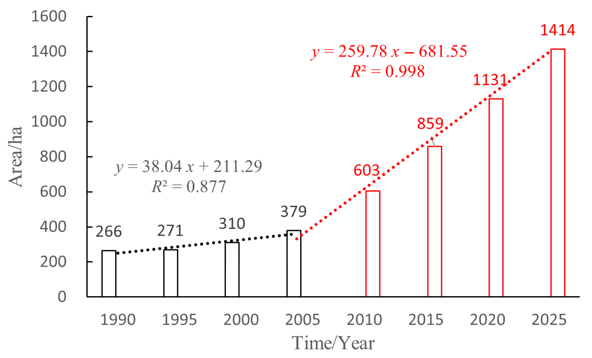
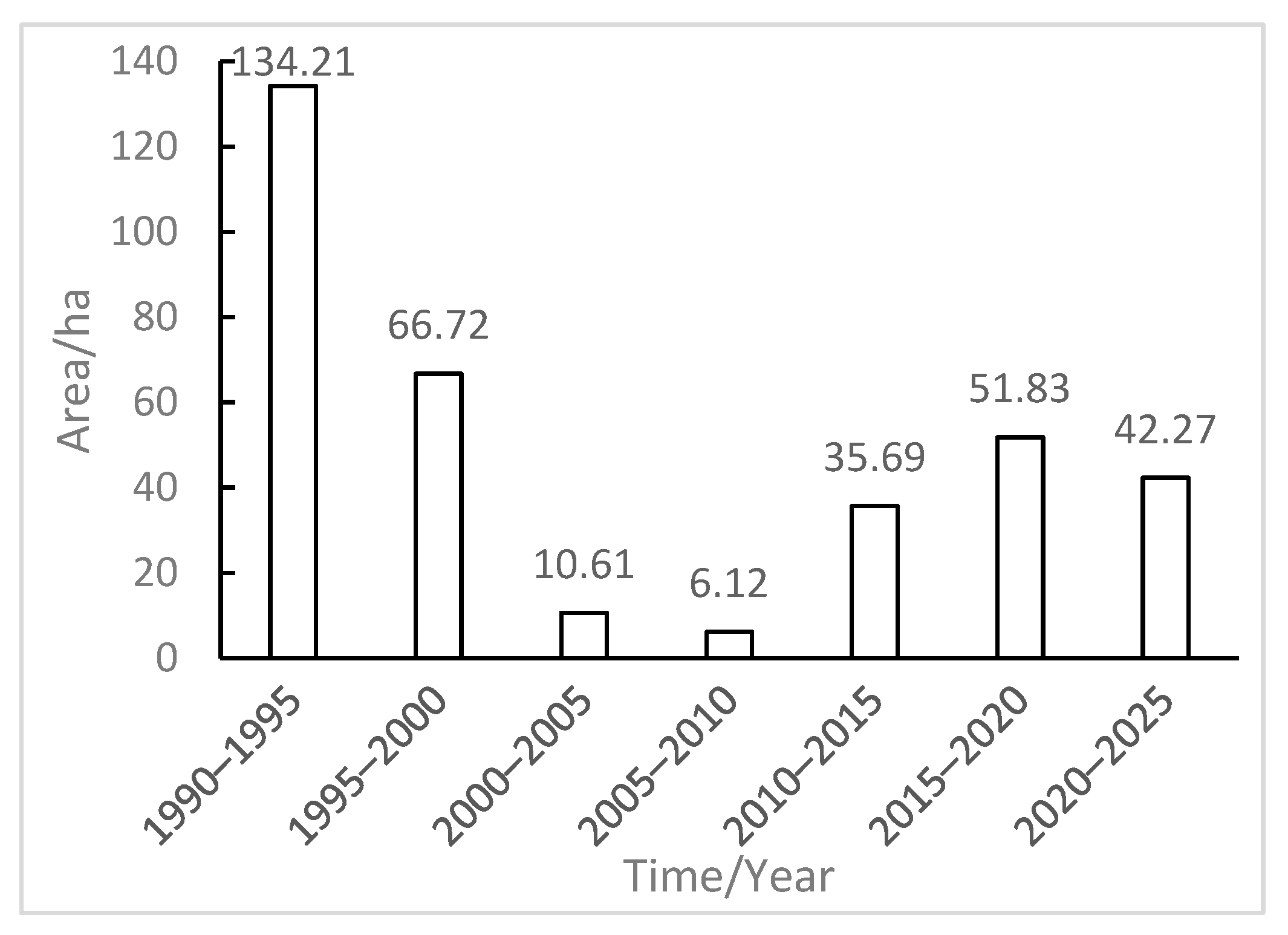
From 1990 to 2025, the total mangrove area in the Nanliu River Delta increased continuously, but the expansion was highly uneven in both time and space. Temporally, the expansion rate was slow before 2005, averaging only 7.61 ha yr⁻¹, whereas it accelerated markedly after 2005, reaching 51.96 ha yr⁻¹ during 2005–2025. Spatially, mangroves expanded predominantly seaward, while landward expansion was strongly constrained by seawall construction and intensive human activities, leaving little available space for further inland migration.

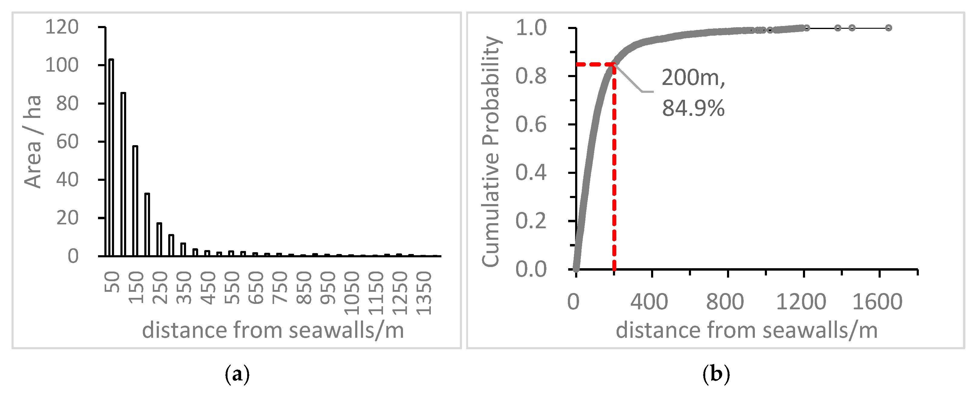
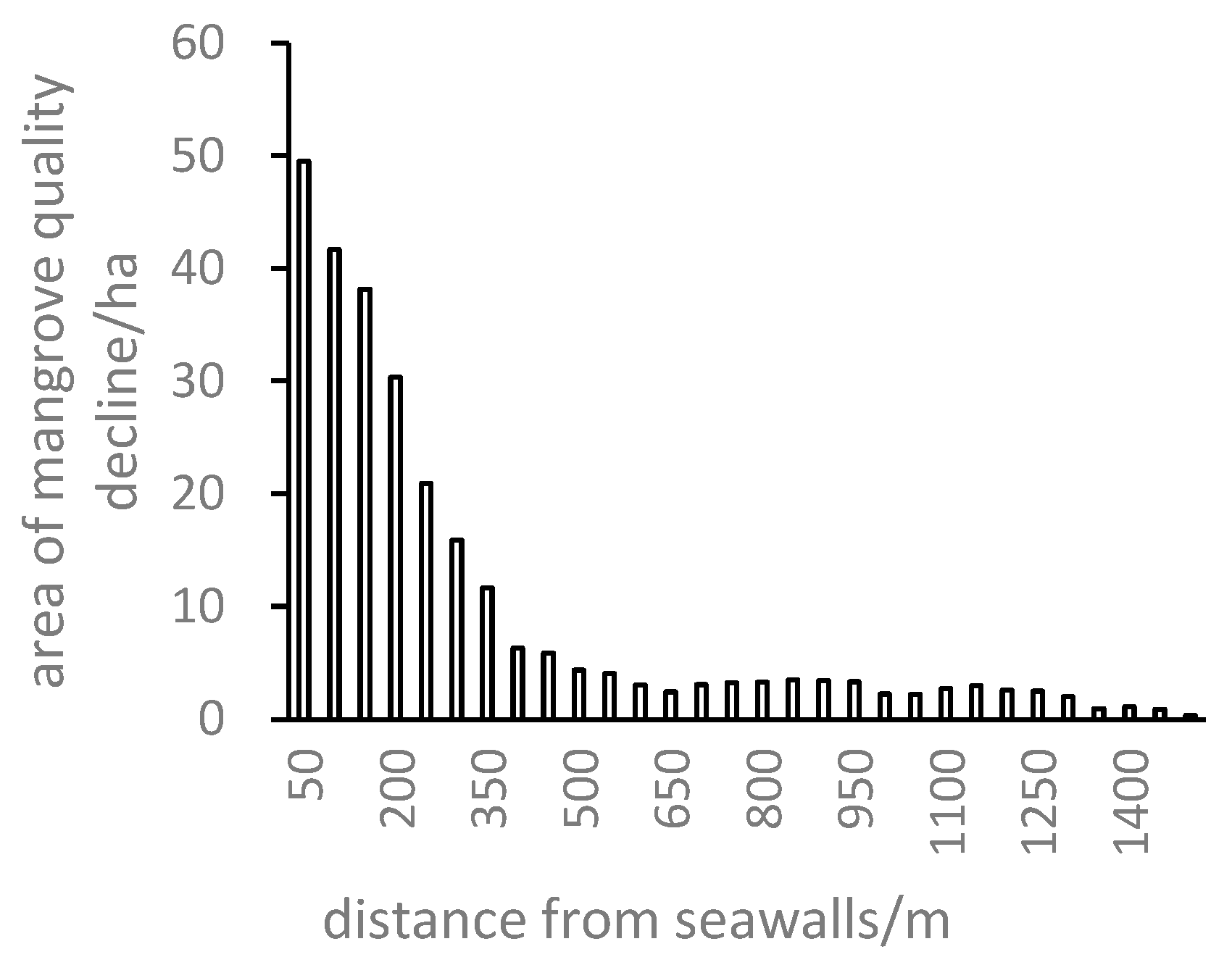
Despite the net gain in mangrove area, localized losses and internal quality decline (ΔEVI decrease) were simultaneously observed, indicating that areal expansion does not necessarily imply functional improvement. Temporally, 57.83% of total mangrove loss (200.93 ha) occurred in the early stage (1990–2000). Spatially, mangrove loss was highly concentrated near seawalls: 82.7% of all losses occurred within the 200 m seawall buffer, and probability density analysis showed that 84.9% of loss pixels were located within 200 m of the seawall.

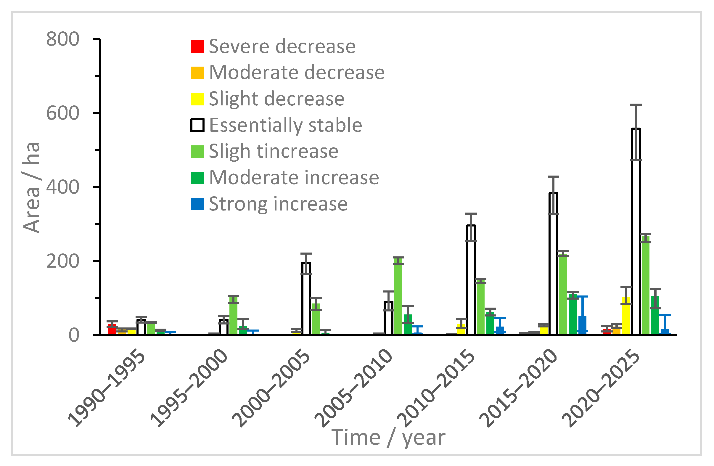
With respect to vegetation condition, mangrove ΔEVI exhibited a clear stage-wise trajectory: pronounced early degradation, followed by mid-term stabilization and rapid recovery, and then a recent phase characterized by the coexistence of recovery and renewed degradation, with increasing areas of slight and moderate decline after 2010. Within 350 m of the seawall, the cumulative area of ΔEVI decrease reached 208.12 ha, accounting for approximately 75.6% of the total degraded area. Overall, ΔEVI decline was highly concentrated within a narrow coastal buffer adjacent to the seawall, forming a distinct inverted-J-shaped distance–risk pattern.

4.2. Plausible Drivers of Mangrove Change

4.2.1. Early-Stage Human Encroachment

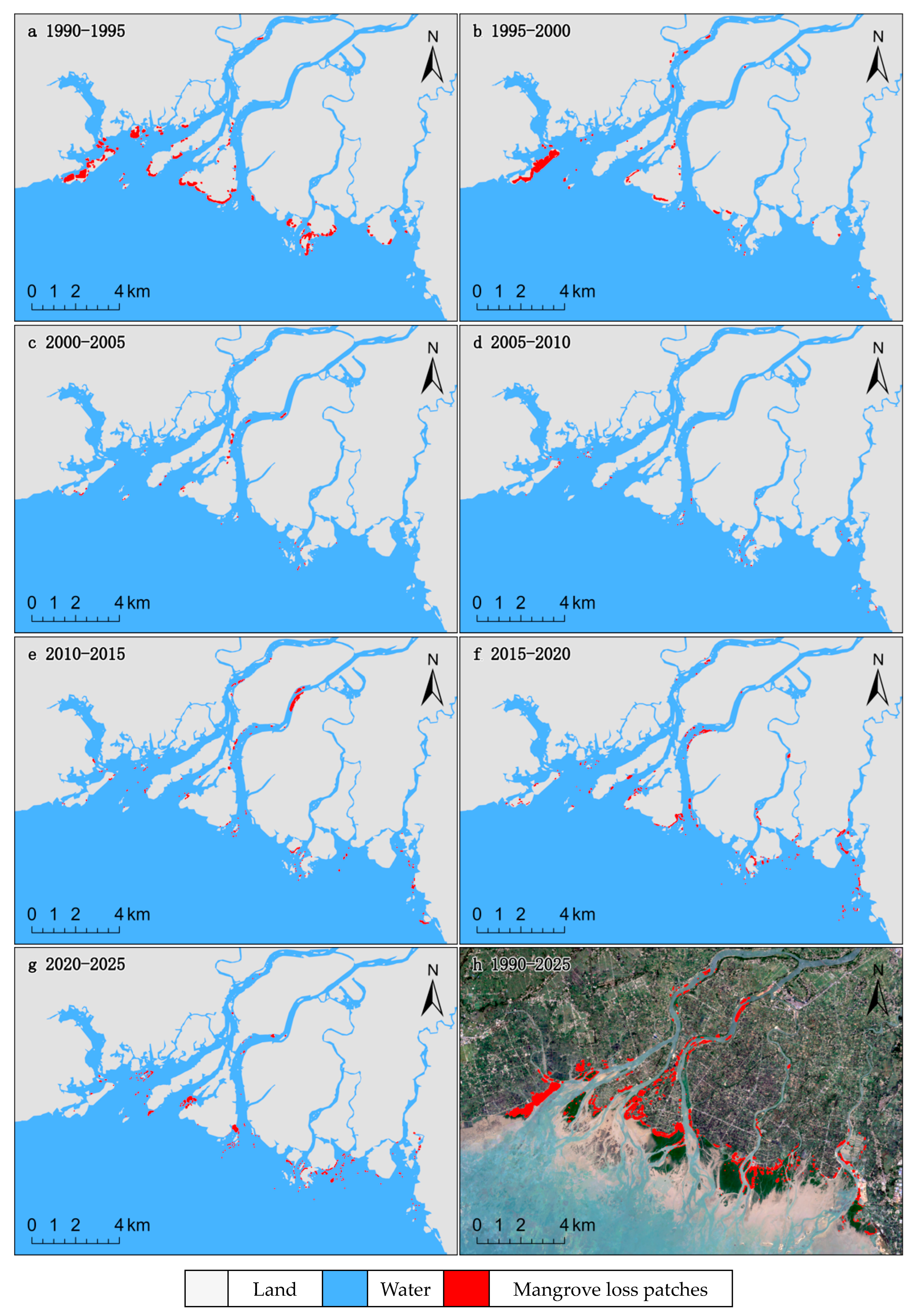
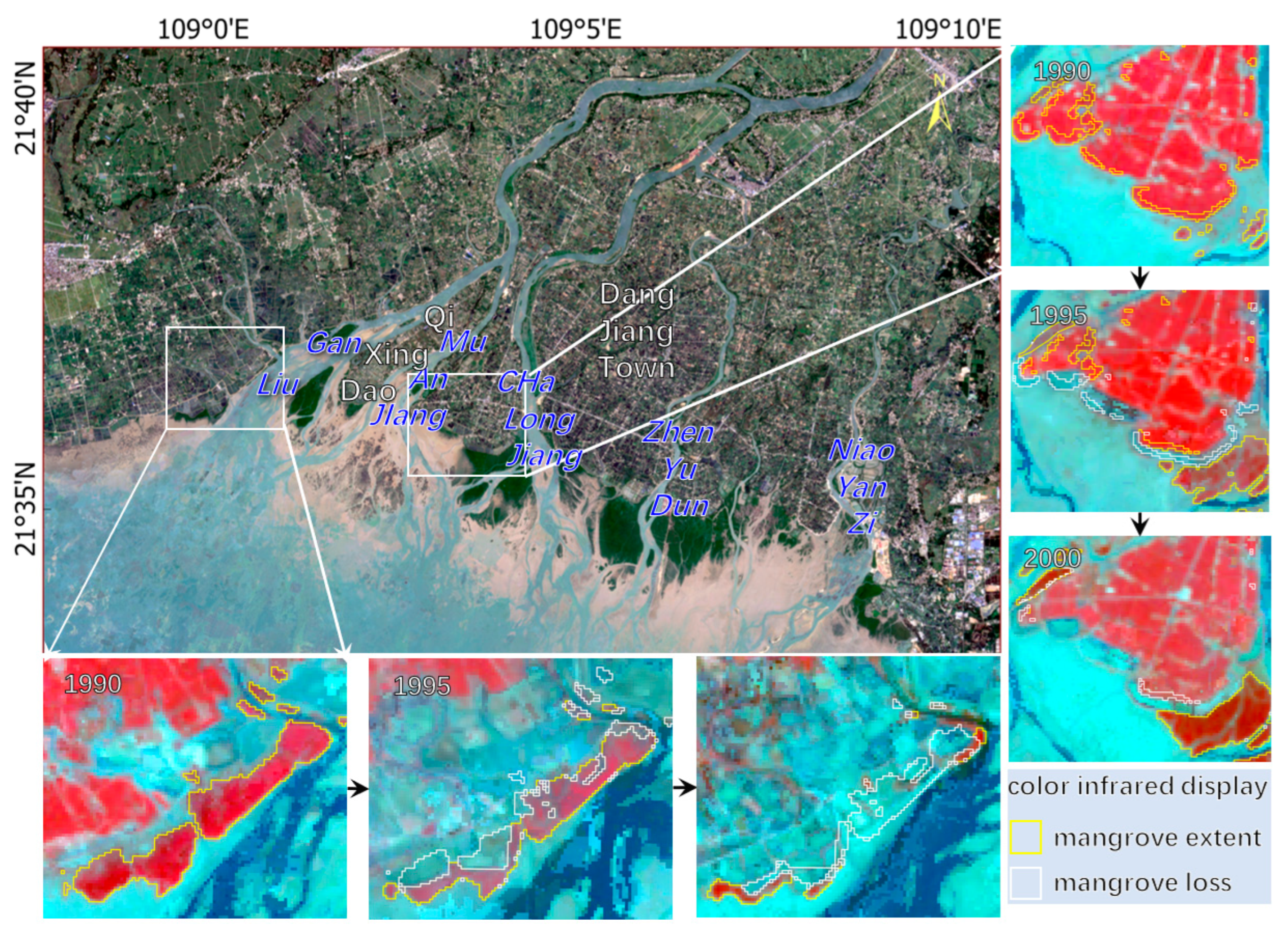
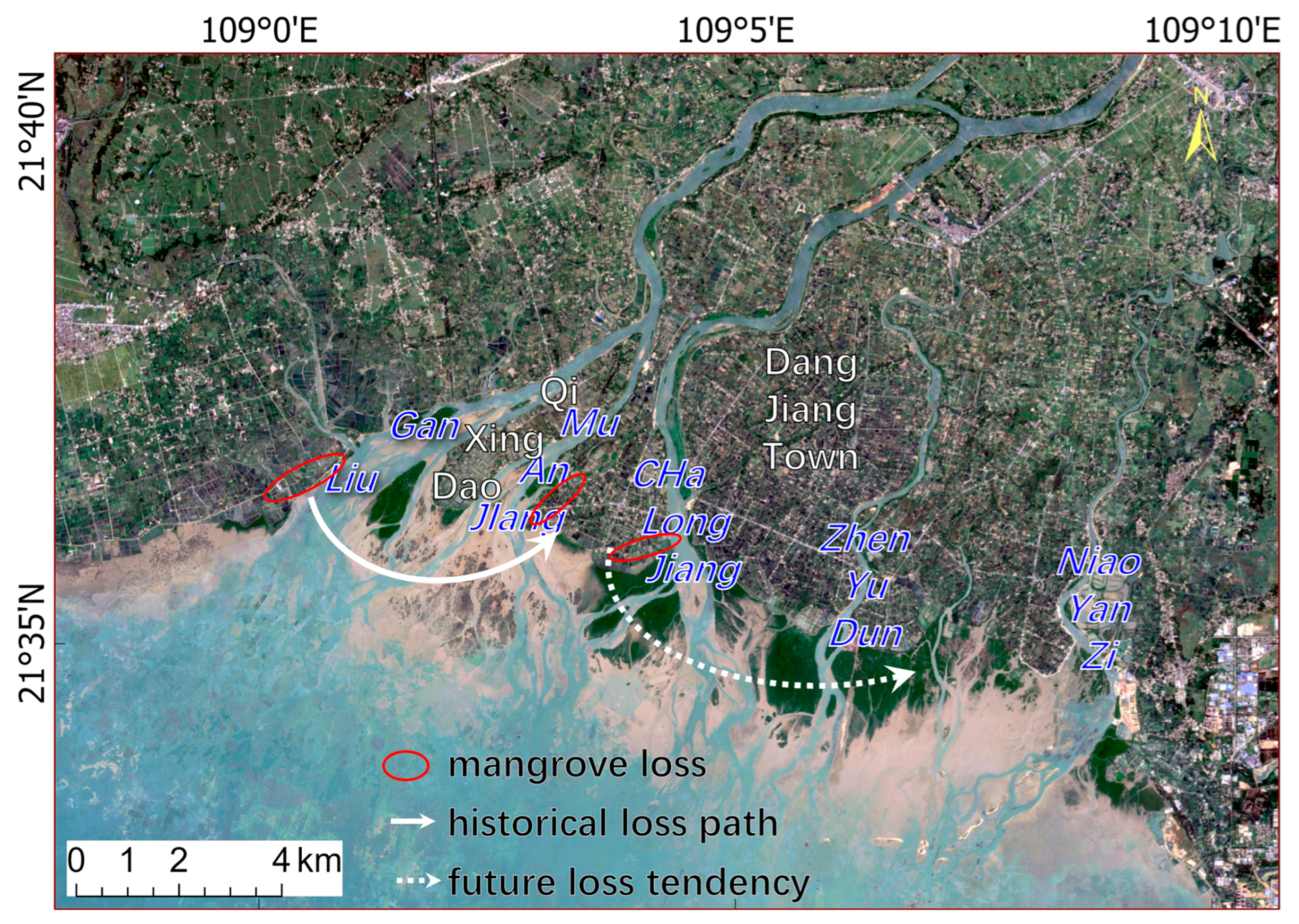
Between 1990 and 2000, mangrove loss in the Nanliu River Delta was spatially concentrated along the western bank of the main stem and the coastal margins of the island bounded by the Muan and Chalong Rivers. During this period, large contiguous mangrove patches disappeared in close proximity to seawalls and engineered shorelines (Figure 13). The spatial configuration and persistence of these losses are consistent with conversion to anthropogenic land uses, such as aquaculture ponds and reclaimed agricultural land, rather than with natural dieback or small-scale canopy disturbance.

Compared with later periods, early losses occurred at larger spatial scales and were more strongly clustered near seawalls, which explains the pronounced inverse J-shaped relationship between mangrove loss and distance from seawalls (Figure 7). This pattern supports the interpretation that shoreline engineering and associated human activities were dominant drivers during the early stage.

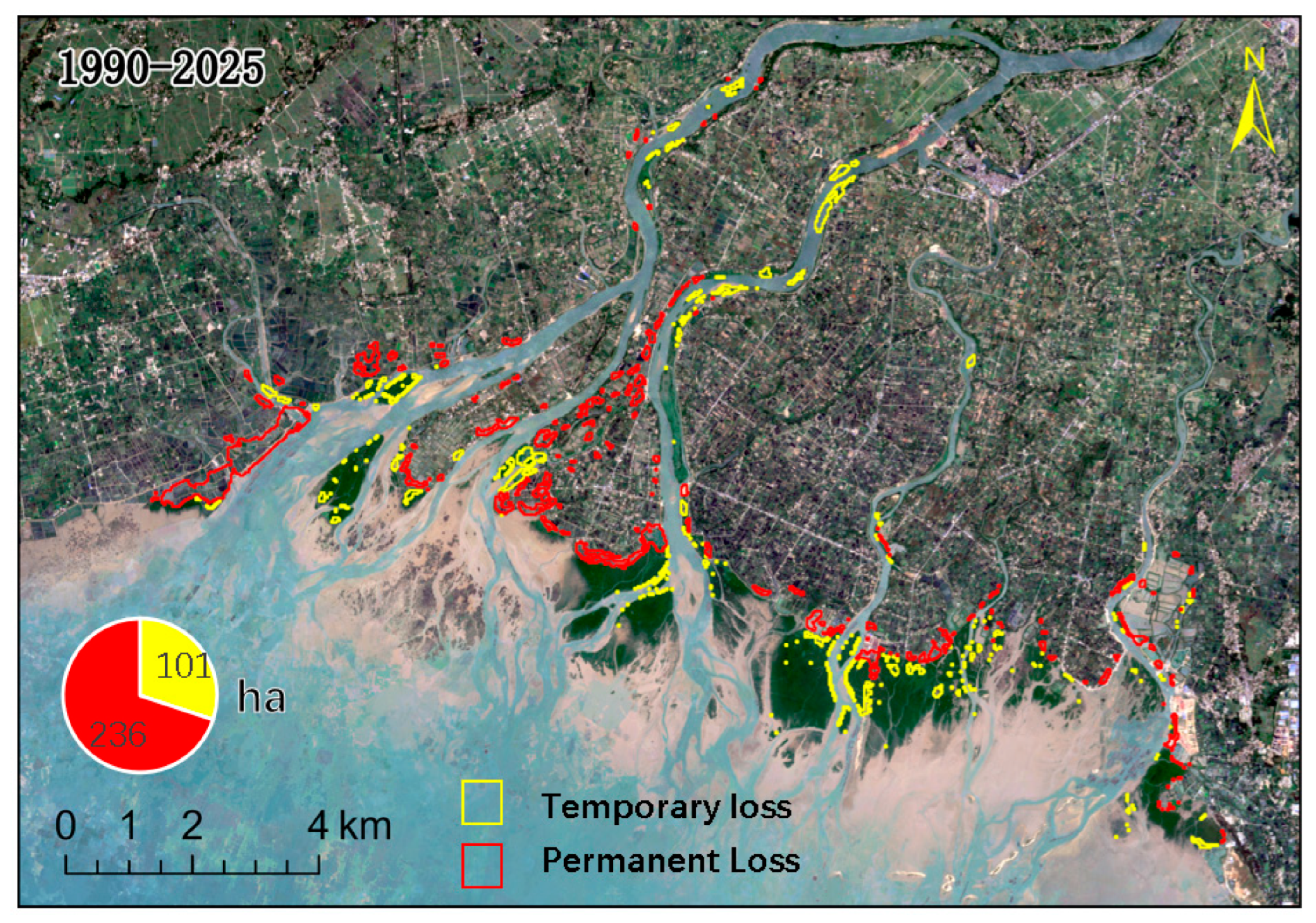
To further examine loss mechanisms, mangrove loss is categorized into two trajectories, Permanent Loss (PL) and Temporary Loss (TL), based on the persistence of land-use change. Permanent loss signifies a fundamental conversion of land use to anthropogenic infrastructure (e.g., aquaculture or coastal engineering), characterized by high socio-economic costs for reversion and negligible natural recovery potential. Temporary loss denotes a transient shift in land cover (e.g., canopy disturbance or selective cutting), where the underlying hydrological and edaphic conditions remain suitable for rapid natural or assisted regeneration. This distinction focuses on the functional reversibility of the site rather than an arbitrary minimum duration.

By classifying mangrove losses across all periods from 1990 to 2025, a mangrove loss-type map for the Nanliu River Delta was produced (Figure 14). Over the 35-year period, 236 ha (~70%) were identified as permanent loss and 101 ha (~30%) as temporary loss. Permanent loss areas were generally closer to seawalls, occurred within more concentrated time windows, and involved larger contiguous areas. Temporary loss accounted for approximately half of the permanent loss area and exhibited a gradually increasing trend.

Previous studies have similarly demonstrated that extensive mangrove degradation at the end of the twentieth century was strongly associated with human activities. For example, Richards and Friess (2016) reported that more than 30% of mangroves in Southeast Asia were lost between 1980 and 2000, with the majority of this loss driven by aquaculture development and agricultural expansion [21]. Along the Chinese coast, particularly in Guangxi and Guangdong provinces, declines in mangrove area have been closely associated with land reclamation and aquaculture activities (Wang et al., 2020) [67]. These findings are consistent with the results of the present study.

4.2.2. Policies for Mangrove Protection and Ecological Restoration

The large-scale occupation of mangrove areas before 2000 coincided with a period of rapid regional economic development and limited regulatory control. In 2000, China launched the Wetland Conservation Action Plan, identifying mangroves as a priority ecosystem for protection. Mangrove area loss declined to its lowest level in that year, marking a critical turning point in the trajectory of mangrove extent in China [68].

Following the implementation of protection and restoration programs, total mangrove area increased rapidly. While this temporal correspondence does not prove causality, the observed trends are consistent with the effects of strengthened conservation policy and restoration initiatives. At the same time, new ecological pressures emerged, particularly near seawalls, where expansion co-occurred with localized decline.

4.3. Observed and Inferable Degradation Processes

4.3.1. Stand Aging as an Intrinsic Source of Vulnerability

Time-series mapping shows that mangroves in the Nanliu River Delta have expanded seaward over the past three decades (Figure 4), implying that landward stands represent earlier-established cohorts with substantially longer stand ages. Many landward mangrove patches have therefore likely exceed ~30 years. Although direct age measurements were not available for all stands, this inference is supported by the spatiotemporal development trajectory of mangrove fronts and the historical stability of landward boundaries constrained by seawalls and human infrastructure.

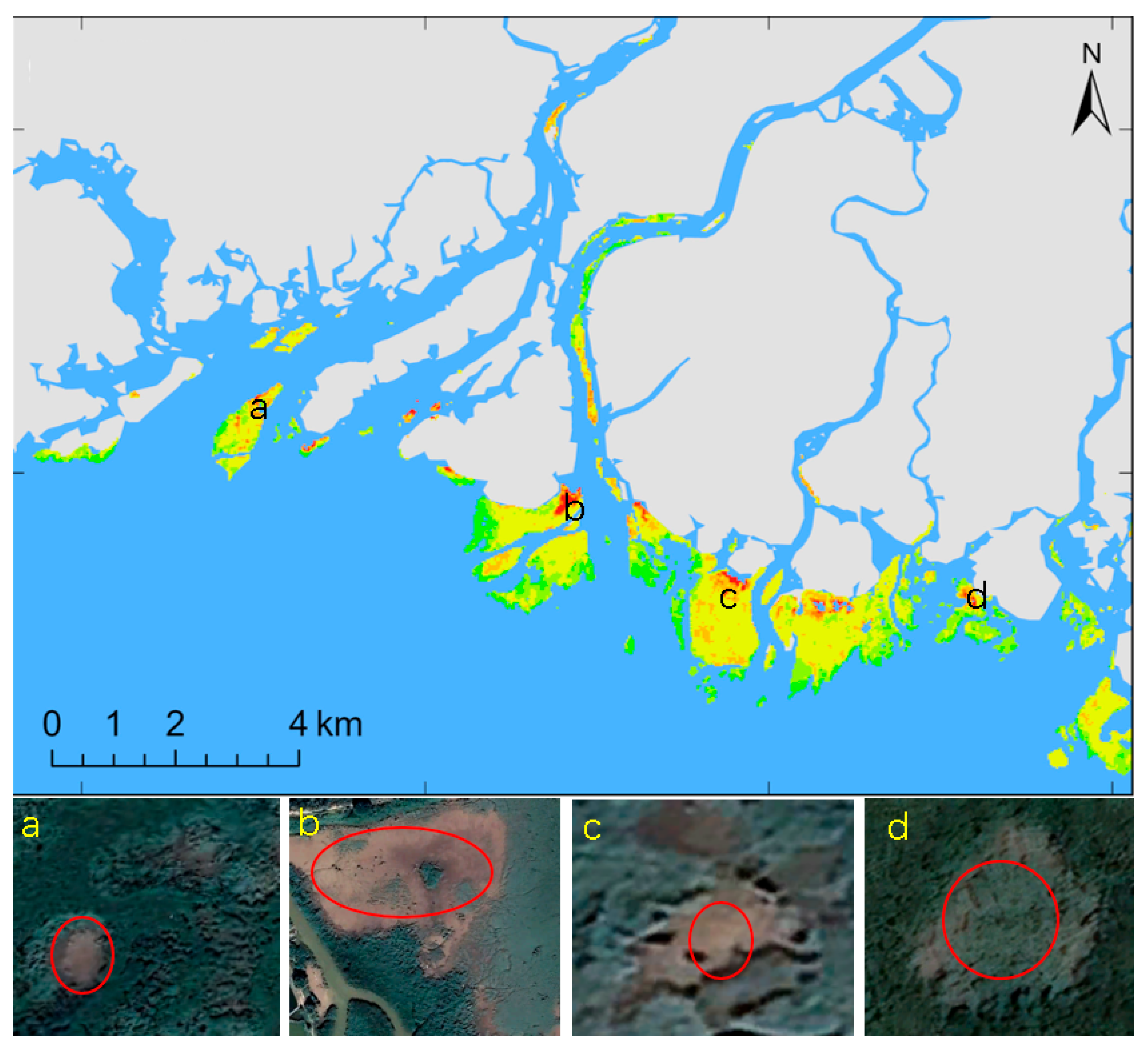
Forest aging is widely recognized as an intrinsic ecological process that can reduce physiological vigor, structural stability, and regenerative capacity. In mangrove ecosystems, advanced stand age is often associated with increased canopy closure, limited understory recruitment, and declining resilience to environmental stress. Our ΔEVI results show that areas with long-standing mangrove presence exhibit a higher probability of slight-to-moderate productivity (Figure 12), consistent with a pattern of gradual functional weakening rather than abrupt clearance.

High-resolution remote sensing imagery from Google Earth reveals the widespread occurrence of canopy gaps within these old mangrove stands (Figure 15).

Importantly, this interpretation does not imply that aging alone causes degradation, but rather that aging increases ecosystem vulnerability.

4.3.2. Field-Observed Biological Stressors and Internal Decline

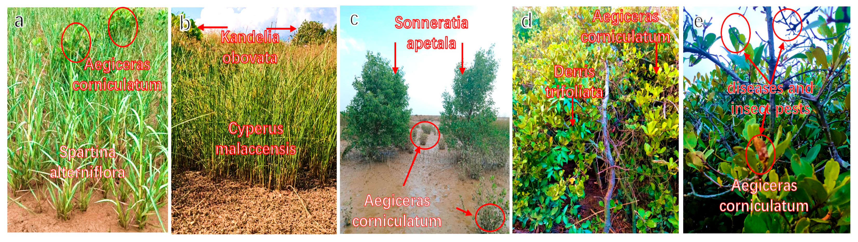
Beyond age-related vulnerability, multiple biological stressors were directly observed during field surveys conducted in 2024–2025. These include (i) invasion by Cyperus malaccensis and Spartina alterniflora, (ii) canopy suppression by the liana Derris trifoliata, and (iii) widespread insect herbivory and foliar disease (Figure 16).

The expansion of Cyperus malaccensis suppresses mangrove seedling survival and regeneration by competing for light and altering sediment structure [69]. Derris trifoliata is a typical climbing plant that can overgrow and smother mangrove canopies, thereby reducing photosynthetic efficiency and, in severe cases, causing large-scale mangrove mortality [70]. In addition, plant diseases and insect pests have shown an intensifying trend, particularly foliar diseases and stem-boring insects, which pose a long-term threat to mangrove regeneration capacity [71,72].

Sonneratia apetala, characterized by its high biomass and exceptional environmental adaptability, was introduced to this region as a fast-growing pioneer species to accelerate afforestation and carbon sequestration. However, its ecological impact is highly context-dependent: while it facilitates initial sediment stabilization on highly dynamic mudflats, it may simultaneously hinder the natural regeneration of native communities in interior zones. The expansion potential of S. apetala is underscored by the nearby Maowei Sea, where it proliferated from zero to 1076.77 ha—now accounting for 50% of the regional mangrove area—within just two decades of its introduction [73]. Consequently, enhanced monitoring and site-specific management strategies are imperative to balance its restoration benefits against potential ecological risks.

Compared with the early phase dominated by externally driven losses caused by direct human encroachment, mangroves in recent decades have increasingly been subjected to degradation pressures originating within the ecosystem itself. These processes do not usually manifest immediately as large-scale, permanent “clear-cut” losses; instead, they emerge gradually in the form of canopy gap formation, community structural degradation, and regeneration failure. Consequently, their impacts on long-term mangrove stability and resilience may be more concealed and persistent.

These stressors represent observed internal degradation processes rather than inferred drivers. They do not necessarily cause immediate mangrove loss but instead contribute to gradual declines in canopy integrity, productivity, and regeneration capacity. Such processes align with the ΔEVI-based patterns of slight and moderate degradation detected in our time-series analysis and help explain why some areas exhibit declining vegetation condition despite stable or increasing mangrove extent.

Together, stand aging and biological stressors form a set of internally mediated degradation mechanisms that are empirically supported by spatial patterns, remote sensing signals, and field evidence.

4.4. Hypotheses for Future Trajectories

Several additional pressures are likely to influence future mangrove condition but cannot be directly quantified in our dataset. These drivers are therefore discussed here as hypotheses supported by external literature and regional context, rather than as confirmed causal factors.

4.4.1. Aquaculture Intensification and Nutrient Loading

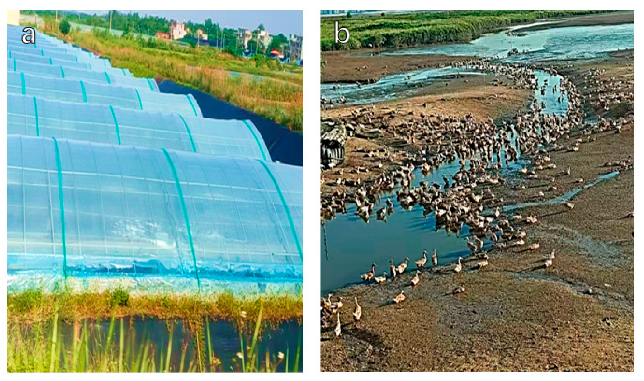
Although large-scale land reclamation and extensive aquaculture have been increasingly restricted by policy since the early 21st century, localized intensive aquaculture and rising cultivation densities—such as high-density shrimp farming (Figure 17a), coastal duck farming (Figure 17b), and associated domestic pollution—continue to alter coastal environments and exert long-term impacts on mangrove ecosystems.

Intensive aquaculture is typically accompanied by the discharge of nutrients (N and P) and organic matter, leading to eutrophication of tidal flats and nearshore waters, reduced dissolved oxygen levels, and altered sediment physicochemical properties [74,75]. These changes affect mangrove rhizosphere environments, soil gas–chemical conditions, and microbial community structures, destabilize the biogeochemical balance, thereby weakening mangrove growth, regeneration, and carbon sequestration functions [76].

Nutrient enrichment also alters competitive dynamics among species. Experimental and regional studies have shown that nitrogen and phosphorus inputs can promote the proliferation and expansion of invasive herbaceous species such as Spartina alterniflora, enabling them to gain spatial dominance and suppress mangrove seedling establishment and regeneration [77].

Organic matter deposition associated with aquaculture increases sediment organic content and the accumulation of reducing substances (e.g., sulfides), alters rhizosphere redox conditions, and may cause root hypoxia or toxicity in mangroves, triggering growth decline or localized mortality [78].

4.4.2. Tourism, Trampling, and Chronic Human Disturbance

In addition, the rise in coastal tourism and recreational tidal-flat harvesting activities has substantially increased pressures such as trampling, vegetation damage, and routine litter deposition [79,80]. These anthropogenic disturbances, particularly the localized harvesting practices in the northern Beibu Gulf, pose a significant threat to the structural integrity of the mangrove ecosystem [79]. Frequent human access directly damages mangrove seedlings and disturbs surface sediments, leading to soil compaction, reduced aeration, and lower re-establishment success rates [81]. Tourism expansion may also alter tidal flow and sedimentation patterns through infrastructure development (e.g., boardwalks, viewing platforms, parking areas), imposing long-term constraints on mangrove recovery.

These pressures are difficult to detect directly using satellite-scale imagery and were not systematically quantified in this study. Therefore, they are presented as emerging and indirect stressors that warrant attention in future monitoring and field-based research, rather than as demonstrated causes of degradation in our results.

4.5. Uncertainty and Temporal Consistency

Several limitations and sources of uncertainty should be acknowledged.

(1)

Sensor-related inconsistencies.

This study integrates multi-decadal Landsat data from different missions (TM, ETM+, and OLI). Subtle inter-sensor differences in spectral response functions may introduce small systematic biases in long-term ΔEVI trajectories. These effects may influence the magnitude of change for individual pixels.

(2)

Tidal-stage dynamics.

Mangrove detection and quality assessment in intertidal environments are inherently sensitive to tidal stage and water level variability. While multi-temporal compositing and robust percentile-based NDVI strategies were used to suppress tidal noise, historical validation data do not allow full control of tidal conditions for all epochs. As a result, residual tidal effects may remain.

(3)

Label dependence and training-data transferability.

The deep learning model was trained primarily using high-confidence reference data from recent epochs. Although geographically diverse global samples were used for pretraining, the application of these labels to earlier periods assumes temporal stability in spectral–structural relationships. This label dependence may propagate uncertainty into early-period maps, especially in areas where species composition or canopy structure has changed substantially over time.

(4)

Spatial autocorrelation and validation bias.

Because mangrove landscapes exhibit strong spatial clustering, random pixel-level train–test splits can inflate accuracy estimates. To reduce this risk, we used geographically independent validation and multi-source cross-checking. Nevertheless, some degree of spatial autocorrelation remains unavoidable at regional scales, and reported metrics should be interpreted as conservative but not fully independent estimates.

(5)

Threshold sensitivity in ΔEVI-based degradation classification.

The classification of degradation levels relies on fixed ΔEVI breakpoints. The ΔEVI thresholds are not intended as universal ecological breakpoints but as relative indicators of canopy vigor change within a consistent sensor and compositing framework. Although these thresholds were informed by literature and empirical interpretation, slight shifts in threshold values (e.g., ±20%) can affect the absolute area of each degradation class. However, sensitivity tests indicate that the relative spatial patterns of decline hotspots and distance–risk relationships remain stable.

Overall, these limitations highlight the need for cautious interpretation and for integrating future field measurements, higher-frequency observations, and long-term ecological monitoring to further refine mangrove quality assessments.

4.6. Management Implications for Estuarine Mangrove Conservation

The results of this study provide several operationally relevant insights for estuarine mangrove management in the Nanliu River Delta and similar coastal systems.

4.6.1. Prioritize Risk Zones Adjacent to Seawalls

Mangrove loss and quality decline are strongly concentrated within narrow buffers along seawalls, forming a clear distance–risk pattern. This indicates that areas within ~200–350 m of coastal embankments should be designated as high-priority management zones. In these areas, routine monitoring, early-warning surveillance, and strict control of adjacent land-use activities (e.g., aquaculture discharge, construction, and access pathways) should be implemented to prevent both direct loss and gradual functional degradation.

4.6.2. Shift Restoration from “Area Expansion” to “Quality-Oriented Recovery”

While total mangrove extent has increased, ΔEVI analyses show that parts of the forest are undergoing physiological and structural degradation. Restoration programs should therefore move beyond simply planting new mangroves and instead focus on improving internal stand condition. This includes thinning over-aged stands where regeneration is suppressed, removing invasive species and climbing plants (e.g., Spartina alterniflora, Derris trifoliata), and enhancing hydrological connectivity to restore sediment and nutrient balance in degraded patches.

4.6.3. Target Quality-Decline Hotspots for Intervention

Spatial clusters of moderate-to-severe ΔEVI decline represent functional degradation hotspots. These areas should be prioritized for field inspection and adaptive management, such as pest control and invasive species removal. Integrating ΔEVI-based early-warning indicators into routine monitoring can enable managers to detect sub-lethal stress before irreversible canopy loss occurs.

4.6.4. Design a Multi-Scale Monitoring Framework

An effective monitoring strategy should combine (i) annual satellite-based ΔEVI screening for long-term trends, (ii) higher-resolution UAV surveys for hotspot validation, and (iii) periodic field assessments for species composition, stand age structure, and regeneration status. This tiered approach allows both broad coverage and fine-scale diagnosis of degradation mechanisms.

4.6.5. Integrate Mangrove Quality into Coastal Planning

Coastal development, aquaculture expansion, and tourism infrastructure should be evaluated not only against mangrove area loss, but also against impacts on mangrove functional condition. Incorporating quality metrics (e.g., ΔEVI trends, regeneration capacity, canopy integrity) into environmental impact assessments can help prevent the silent erosion of ecosystem services even where forest extent appears stable or increasing.

Overall, the findings highlight that sustainable mangrove management in estuarine systems requires a dual focus on where mangroves are and how well they function. The combination of spatial risk zoning, quality-oriented restoration, and multi-scale monitoring provides a practical pathway for translating remote sensing diagnostics into actionable conservation strategies.

5. Conclusions

5.1. Methodological Contribution

This study developed a time-series mangrove mapping framework that integrates NDVI-PP75 compositing with deep learning to improve the extraction of mangrove extent and degradation signals from long-term Landsat imagery. The results demonstrate that the proposed approach is capable of consistently capturing historical mangrove dynamics in complex deltaic and intertidal environments.

5.2. Mapping Performance

The proposed framework achieved high and stable classification accuracy. For the mangrove class, Precision, Recall, and F1-score reached 0.910, 0.895, and 0.902, respectively, corresponding to an IoU of 0.822. For the background class, Precision, Recall, and F1-score were 0.990, 0.992, and 0.992, with an IoU of 0.981. The mean IoU (mIoU) across both classes was 0.902.

5.3. Key Spatiotemporal Trends

Mangrove area in the Nanliu River Delta increased from 266 ha in 1990 to 1414 ha in 2025. Temporally, the expansion rate was modest before 2005 (7.61 ha yr⁻¹ on average) and increased substantially during 2005–2025 (51.96 ha yr⁻¹). Spatially, expansion occurred predominantly seaward, while landward migration was strongly constrained by seawall construction and intensive human activities, leaving limited space for further inland colonization.

Over the study period, total mangrove loss amounted to 347.45 ha. Notably, 57.83% of this loss (200.93 ha) occurred during the early stage (1990–2000). Approximately 70% (236 ha) of the mangrove loss was converted to built-up and agricultural land, primarily for aquaculture ponds and coastal engineering infrastructure.

5.4. Seawall-Risk Pattern

Both mangrove loss and quality decline exhibited a strong inverse J-shaped relationship with distance to seawalls, consistent with a pronounced “coastal squeeze” effect. Specifically, 82.7% of all losses occurred within the 200-m seawall buffer, and probability density analysis showed that 84.9% of loss pixels were located within 200 m of the seawall, indicating that the most intense human disturbance is largely confined to a narrow coastal strip. Within 350 m of the seawall, the cumulative area of ΔEVI decrease reached 208.12 ha (≈75.6% of the total ΔEVI degraded area), potentially linked to stand aging.

5.5. Management Relevance

Overall, the proposed framework provides a scalable and transferable tool for long-term mangrove monitoring using freely available satellite data. It supports integrated assessments of both mangrove quantity and quality, offering valuable scientific evidence for blue carbon evaluation and adaptive coastal management. Future studies should further incorporate higher-resolution imagery and field-based ecological measurements to strengthen the linkage between remotely sensed indicators and underlying biophysical processes.