Ecological Water Requirements and Ecosystem Responses in the Downstream Reaches of a Typical Arid Inland River Basin

Abstract

The Three-River Connectivity Zone in the lower Tarim River Basin (TRCZ) is a typical area that has experienced decades of river cut-off, followed by artificial ecological water transfers and vegetation restoration. However, the long-term patterns of ecological water requirements and their response mechanisms to ecosystem services in this region remain unclear. This study aims to quantify the spatiotemporal dynamics and driving factors of ecological water requirements in the TRCZ from 1990 to 2020. We integrated multi-temporal remote sensing land cover data with the FAO Penman–Monteith equation to estimate vegetation evapotranspiration (as a proxy for ecological water requirement) and coupled the InVEST model with Random Forest modeling to identify key climatic and hydrological drivers. Unlike previous studies that focused primarily on precipitation inputs, our approach explicitly considers the ecosystem’s water yield function alongside water demand, offering new insights into the constraints on ecosystem services. Key findings reveal: (1) During the period of 2005–2010, the land cover types underwent significant changes, characterized by a marked expansion of sparse forest (14–21%) and a pronounced decline in forest land, which fundamentally reconfigured the ecosystem’s water demand structure. (2) Accordingly, the multi-year average ecological water requirement quota in the study area is 2.95 × 10⁷ m³, and the total ecological water requirement exhibited a fluctuating decline at a rate of −1.39 × 10⁵ m³/yr, yet sparse forest persisted as the dominant water-consuming component. (3) The Random Forest model (R² = 0.942) identified water yield (importance: 0.527) and precipitation (0.255) as the primary drivers, establishing the ecosystem’s water yield function rather than precipitation input alone as the critical constraint. (4) A widespread increase in the unit area ecological water requirement across vegetation types signaled escalating pressures from climate change. This research provides a quantitative framework and a transferable methodology for adaptive water resource management and ecological restoration in arid regions, emphasizing the balance between ecosystem water demand and supply functions.

1. Introduction

Ecological water requirements constitute a central issue in water resource management, as they directly underpin the balance between ecosystem conservation and regional sustainable development [1,2,3]. In arid regions, where precipitation is extremely scarce and water availability is severely constrained, rivers frequently experience seasonal or periodic flow interruptions. Consequently, the downstream ecosystems exhibit heightened sensitivity to hydrological deficits and have particularly stringent water demands [4]. Riparian vegetation and associated ecological communities depend on stable streamflow to sustain biodiversity, maintain ecological function, and ensure habitat integrity. However, excessive water withdrawal and inefficient water use, compounded by high losses during conveyance and application, especially for agricultural irrigation, urban consumption, and industrial production, have resulted in diminished river discharge, degradation of riparian vegetation, and persistent declines in groundwater levels. In several arid basins, prolonged water shortages have led to drastic wetland shrinkage and, in some cases, irreversible ecological degradation. Therefore, ensuring adequate ecological water allocation has become a top priority in the management of water-limited environments. In recent years, growing recognition of ecosystem vulnerability has prompted many regions to implement a range of ecological restoration measures. These include the establishment of ecological flow regimes, wetland rehabilitation, and artificial water supplementation, all of which are aimed at balancing human water use with the long-term stability of ecosystem functions [5,6]. Integrated management and scientifically informed planning of water resources have emerged as key pathways for achieving harmonious coexistence between human activities and natural ecosystems in arid regions. Through rational water allocation, such regions can not only improve their ecological conditions but also enhance water-use efficiency and promote sustainable regional development.

Quantifying the hydrological conditions required to sustain ecosystem health and service functions is the core objective of ecological water requirement assessments. Existing research, both in China and internationally, has focused extensively on the development of quantitative methodologies, leading to the establishment of hydrological, hydraulic, and habitat-simulation approaches. In arid basins, the ecological water requirement is strongly and positively associated with ecological carrying capacity, with particularly tight linkages observed in forest and grassland ecosystems [7,8]. However, traditional methods often encounter limitations when applied to inland river basins in arid regions, largely due to the high diversity of vegetation types and pronounced differences in phenological stages, which hinder fine-scale estimation. Compared with these conventional approaches, the FAO Penman-Monteith equation, which incorporates vegetation coefficients, soil moisture stress factors, and distinctions among phenological periods, substantially enhances the accuracy of ecological water requirement calculations [9,10]. Research on ecosystem services has exhibited a notable shift from global-scale assessments to medium- and small-scale analyses of complex ecosystem mosaics, encompassing forests, grasslands, wetlands, and urban systems [11,12]. Research priorities have evolved from foundational work on conceptual frameworks and classification systems to more applied investigations emphasizing ecosystem service assessment and valuation, their dependence on human well-being, and their responses to climate change, land cover transitions, and anthropogenic disturbances [13,14]. The relationship between ecological water requirements and ecosystem services has attracted growing attention. Recent studies have highlighted the critical role of ecohydrological feedback in regulating peatland water storage, baseflow, and drought resilience, thereby elucidating the mechanisms through which ecological water inputs support services such as water regulation and climate moderation [15]. Additionally, increasing emphasis is being placed on understanding the spatial mismatches between ecosystem service supply and demand, as well as the processes governing service flows. Identifying priority service supply areas and optimizing spatial resource allocation have proven effective in alleviating supply demand conflicts and offer new perspectives for the refined management of ecological water allocation [16]. Despite these advances, research on the coupling mechanisms between ecological water requirements and ecosystem service functions at the watershed-scale in arid regions remains relatively limited. Existing studies often focus on individual variables or localized processes and lack a systematic analysis of the integrated “water-vegetation-services” nexus. This gap constrains the development of ecosystem service-oriented strategies for precision ecological water allocation [17]. Therefore, investigating the linkages between ecological water requirements and ecosystem service functions in arid region basins has substantial scientific value. Such efforts can deepen our understanding of ecohydrological processes and service formation mechanisms, while providing critical theoretical support for integrated watershed management that simultaneously enhances water use efficiency and ecological conservation.

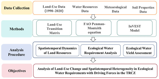
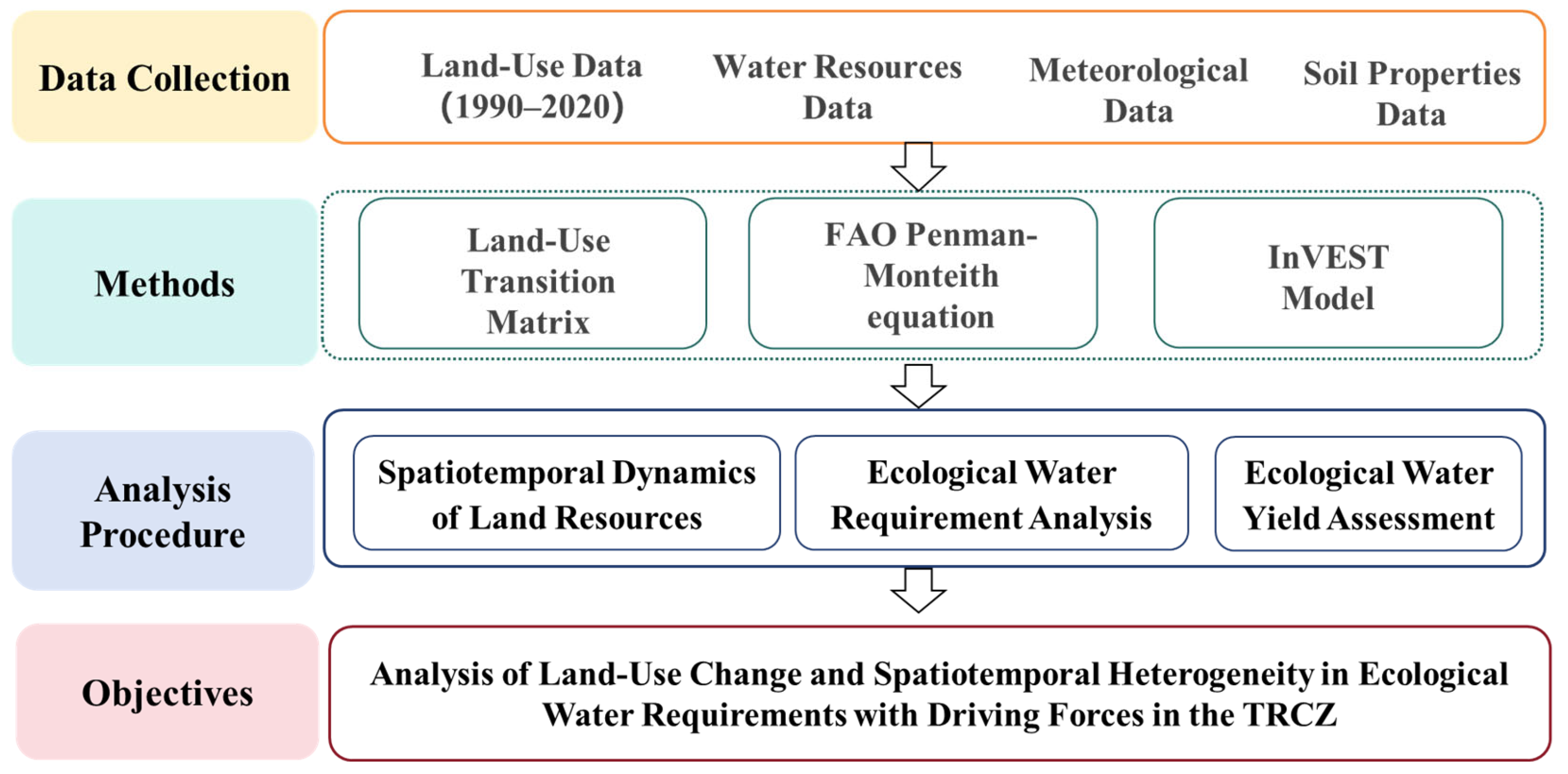
The Three-River Connectivity Zone in the lower Tarim River Basin (TRCZ) encompasses the downstream sections of the Tarim, Kongque, and Nashen Rivers, where the landscape is dominated by alluvial plains, low hills, and extensive desert terrain. Situated within the influence of the Taklimakan and Kuruk Deserts, the region exhibits a typical temperate continental arid desert climate, resulting in an exceptionally fragile ecological environment and severe water scarcity [18]. Driven by climatic factors and intensified human activities, approximately 350 km of the lower Tarim River has experienced channel desiccation since the 1950s, leading to the complete drying of the terminal lakes, Lop Nur and Taitema Lake, and the continuous shrinkage of Populus euphratica forests [19,20]. Under these conditions, ecological water allocation is critical for both ecosystem restoration and channel rehabilitation. The effectiveness and long-term sustainability of ecological restoration efforts depend fundamentally on the rational distribution of ecological flows, with stable water yield representing a core prerequisite. In response to the near collapse of the lower Tarim River ecosystem, the Chinese government initiated large-scale ecological water conveyance in 2000, with an average annual delivery volume of 4.32 × 10⁸ m³ by 2018. Nevertheless, vegetation recovery remains largely confined to within 1 km of the river channel, and the overall ecological improvement remains limited [21]. Given the constraints on total ecological water availability, improving the precision of vegetation water demand estimates, enhancing water use efficiency, and expanding the effective restoration area have become urgent priorities for ecological management in this region. In this study, “sustainable management” refers to long-term, adaptive ecological water allocation combined with land-cover protection/optimization to maintain ecosystem functions under persistent water scarcity, rather than short-term engineering interventions alone. To address these challenges and characterize vegetation water requirements with greater accuracy, this study aims to resolve the following key scientific questions (Figure 1):

(1)

To reveal the spatiotemporal patterns of land cover change in TRCZ, using multi-temporal land use/land cover (LULC) remote sensing data to quantify land cover composition dynamics and identify transition processes among vegetation-dominated land cover types;

(2)

To quantify ecological water requirements for major vegetation types, calculating vegetation water demand during distinct growing-season phenological periods (initial growth stage, development stage, mid-growth stage, and late-growth stage) from April to October for 1990–2020 using FAO Penman-Monteith equation, and elucidating their spatiotemporal variability;

(3)

To identify the dominant drivers of ecological water requirement, applying a random forest model to assess the response relationship between vegetation water requirements and water yield conditions, and to propose sustainable water-soil resource regulation strategies that support stable ecosystem restoration in the downstream region.

2. Materials and Methods

2.1. Study Area

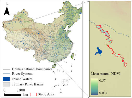
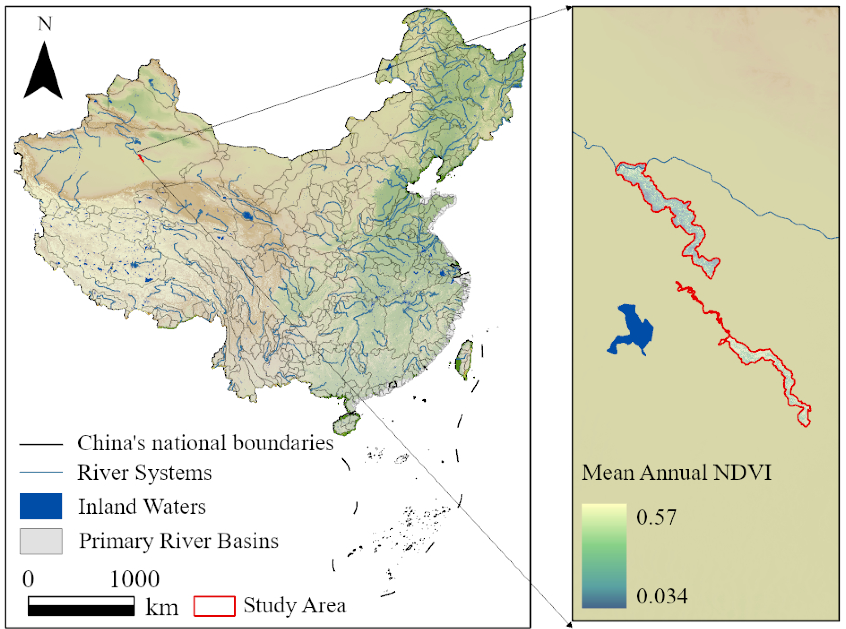
TRCZ encompasses the downstream sections of the Tarim, Kongque, and Nashen Rivers, where the landscape is dominated by alluvial plains, low hills, and desert terrain (Figure 2). Located within the influence range of the Taklimakan and Kuruk Deserts, the region is characterized by an arid climate with scarce precipitation, strong evaporation, and frequent winds during spring and autumn [22]. Annual precipitation is extremely low, ranging from only 17.4 to 42.0 mm, whereas potential evaporation reaches 2500–3000 mm. This typical temperate continental arid desert climate results in a highly fragile ecological environment with severe water scarcity. Under such conditions, ecological water allocation plays a critical role in ecosystem restoration and riverine management [23].

2.2. Methods

2.2.1. Land Cover Dynamics and Transition Matrix

The land cover transition matrix enables a quantitative assessment of conversion among different land cover categories (derived from multi-temporal land use/land cover data), providing an intuitive representation of transformation trends between land-cover types [24]. Its mathematical expression is given as follows:

$$D_{xy}=\left[\begin{array}{cccc}{D}_{11}& D_{12}& \dots & D_{1n}\\ D_{21}& D_{22}& \dots & D_{2n}\\ ⋮& ⋮& \ddots & ⋮\\ D_{n1}& D_{n2}& \dots & D_{nn}\end{array}\right]$$

(1)

where $D$ represents the area of each land cover type (km²), $x$ and $y$ denote the land cover types before and after the transition, respectively, and $n$ is the total number of land cover categories within the study area.

2.2.2. Estimation of Ecological Water Requirement Quotas

The conventional Penman equation typically estimates vegetation water demand under ideal conditions, assuming sufficient water supply, adequate fertilization, and the absence of pests or diseases in the vegetation. Under these assumptions, the calculated value represents the maximum ecological water requirement of vegetation, rather than the actual water needed to sustain plant survival. The FAO Penman-Monteith equation estimates the actual water demand of vegetation by calculating potential evapotranspiration and adjusting it using vegetation and soil stress coefficients. In this study, by integrating the area quota method, FAO Penman-Monteith equation, soil moisture restriction coefficient, and vegetation coefficient, the ecological water requirement of the study area was set as [25]:

$$W=E{T}_k\times A_k$$

(2)

where $W$ denotes the total ecological water requirement of vegetation (10⁸ m³), $E{T}_k$ is the water demand quota of vegetation type $k$ (mm), and $A_k$ represents the area of vegetation type $k$ (m²).

(1)

Evapotranspiration Calculation

The reference crop evapotranspiration ($E{T}_k$) was calculated using the FAO Penman-Monteith equation, as shown in Equation (4). The actual evapotranspiration of the vegetation was obtained using Equation (3):

$$E{T}_k=E{T}_0\times K_s\times K_c$$

(3)

where $E{T}_0$ is the reference crop evapotranspiration (mm), $K_s$ is the soil moisture stress coefficient, and $K_c$ is the vegetation coefficient for vegetation type $k$.

The Penman-Monteith equation is expressed as:

$$E{T}_0={\displaystyle \frac{0.408\Delta \left(R_n-G\right)+r\frac{900}{T+273}{u}_2\left(e_s-e_a\right)}{\Delta +r\left(1+0.34u_2\right)}}$$

(4)

where $E{T}_0$ is the reference crop evapotranspiration (mm/d), $\Delta$ is the slope of the saturation vapor pressure curve (kPa/°C), $G$ is the soil heat flux (MJ·m⁻²·day⁻¹), $\gamma$ is the psychrometric constant (kPa/°C), $u_2$ is the wind speed at 2 m height (m/s), $e_s$ is the saturation vapor pressure (kPa), $e_a$ is the actual vapor pressure (kPa), and $R_n$ is the net radiation at the surface (MJ·m⁻²·day⁻¹).

(2)

Soil Moisture Stress Analysis

The soil moisture stress coefficient (also referred to as the wilting coefficient) is primarily influenced by soil texture. Based on soil impact data from 42 meteorological stations in Xinjiang, a long-term average value of 0.36 was adopted as the representative value of the $K_s$ for the lower reaches of the Tarim River.

(3)

Vegetation Coefficient

The vegetation coefficient ($K_c$) is a function of vegetation cover, height, and leaf area index, and it varies with the phenological stages of plant growth. In the lower Tarim River region, the vegetation coefficients for different plant types were determined based on the ratio of leaf area index at the initial and late-growth stages to that at the mid growth stage. According to previous studies, the growing season of vegetation in Xinjiang spans from April to October. The growth stages are classified as early growth (April), development stage (May–June), mid-growth stage (July–September), and late-growth stage (October), which were used to define the growth patterns and vegetation coefficients for each vegetation type (

Table 1. Growing-Season Periods and Vegetation Coefficients for Different Vegetation Types.

Vegetation Type	Early Growth (April)	Development Stage (May–June)	Mid-Growth Stage (July–September)	Late-Growth (October)
Forested Land	0.53	1.04	1.13	0.97
Shrubland	0.19	0.33	0.58	0.60
Sparse Forest	0.20	0.52	0.91	0.78
Other Forests	0.45	0.55	0.85	0.60
High-Coverage Grassland	0.23	0.44	0.55	0.45
Medium-Coverage Grassland	0.15	0.20	0.30	0.25
Low-Coverage Grassland	0.11	0.18	0.25	0.15

) [26,27]. In this article, ‘growth stage’ refers to within-year growing-season phenological periods (time of year) rather than forest age or stand development stage.

2.2.3. Water Yield Function Simulation

The water yield function in the study area from 1990 to 2020 was simulated using the InVEST model to further elucidate the logical relationship between the ecological water requirement and water yield. The water yield function is defined as follows:

$$Y_{xj}=\left(1-{\displaystyle \frac{{AET}_{xj}}{P_x}}\right)\times P_x$$

(5)

where $Y_{xj}$ represents the water yield (mm) of grid cell $x$ for land cover type $j$, calculated as the precipitation minus actual evapotranspiration; ${\mathit{AET}}_{xj}$ is the actual evapotranspiration (mm) of grid cell $x$ for land cover type $j$; and $P_x$ denotes the annual precipitation (mm) of grid cell $x$.

$${\displaystyle \frac{{AET}_{xj}}{P_x}}={\displaystyle \frac{1+{\omega }_x{R}_{xj}}{1+{\omega }_x{R}_{xj}+1/R_{xj}}}$$

(6)

$$R_{xj}={\displaystyle \frac{K_{xj}\times {ET}_{0x}}{P_x}}$$

(7)

$${\omega }_x=Z{\displaystyle \frac{AW{C}_x}{P_x}}$$

(8)

$$AW{C}_x=min\left(MaxSoilDept{h}_x,RootDept{h}_x\right)\times PAW{C}_x$$

(9)

where $R_{xj}$ is the aridity index of grid cell $x$ for land cover type $j$, representing the ratio of potential evapotranspiration ($E{T}_{0x}$) to precipitation ($P_x$); $K_{xj}$ is the vegetation evapotranspiration coefficient; ${\omega }_x$ is a dimensionless, non-physical parameter representing soil properties under natural climatic conditions; $Z$ is the seasonal Zhang coefficient, characterizing regional hydrogeological conditions; $AW{C}_x$ is the plant available volumetric water content, i.e., the effective soil water content of grid cell $x$ (mm); $MaxSoilDept{h}_x$ is the maximum soil depth; $RootDept{h}_x$ is the root depth; and $PAW{C}_x$ is the plant available water.

2.2.4. Random Forest Algorithm (RF)

RF consists of multiple decision trees. Under the condition of a given independent variable X, the predictive outcomes of each decision tree are aggregated through voting or averaging to select the optimal classification result. During the construction of each decision tree, a bootstrap sampling method is used to generate random subsets of samples, which are then utilized to build the ensemble of decision trees and consolidate their predictions. When the model is applied to regression prediction, the result is the average of the predicted outcomes from all decision trees [28]. In this study, the method was employed to investigate the driving factors influencing ecological water requirements.

Accuracy Verification: This study employed the K-fold cross-validation method, the core concept of which is to randomly partition the original dataset into K mutually exclusive subsets of equal size. In each iteration, K-1 subsets are selected as the training set to construct the model, while the remaining one subset serves as the validation set to evaluate the model’s performance. Three metrics—the coefficient of determination (R²), root mean square error (RMSE), and mean absolute error (MAE)—are chosen to assess the model’s performance. The formulas for these metrics are as follows:

$$R^2={\left({\displaystyle \frac{{\sum }_{i=1}^n\left(O_i-\overline{O}\right)\left(M_i-\overline{M}\right)}{\sqrt{{\sum }_{i=1}^n{\left(O_i-\overline{O}\right)}^2}\sqrt{{\sum }_{i=1}^n{\left(M_i-\overline{M}\right)}^2}}}\right)}^2$$

(10)

$$RMSE=\sqrt{{\displaystyle \frac{{\sum }_{i=1}^n{\left(O_i-M_i\right)}^2}{n}}}$$

(11)

$$MAE={\displaystyle \frac{1}{n}}{\sum }_{i=1}^n\left|{M_i-O}_i\right|$$

(12)

where $O_i$ is the actual value, $M_i$ is the predicted value, $n$ is the sample size, $\overline{O}$ is the mean of the actual values, and $\overline{M}$ is the mean of the predicted values.

2.3. Data

The data required for this study are listed below (

Table 2. Data Required for the Study.

Data Type	Explanation	Data Source
Land Use Data	Comprises 7 periods from 1990 to 2020 (1990, 1995, 2000, 2005, 2010, 2015, 2020). Resolution: 30 m, yearly data.	Resource and Environmental Science Data Platform of Chinese Academy of Sciences (RESDC, https://www.resdc.cn/ (accessed on 28 September 2025))
NDVI Data	Used to delineate the vegetation extent within the study area. Resolution: 30 m, yearly data.
Climate Background Data	Includes multi-year average data for 9 climate factors: Precipitation, Temperature, Sunshine Duration, Atmospheric Pressure, Solar Radiation, Surface Temperature, Wind Speed, Evaporation, and Relative Humidity. Resolution: 1000 m.
Potential Evapotranspiration, Precipitation, and Temperature Data	Used to drive the water yield module of the InVEST model for calculating meteorological factors, rainfall erosivity, etc. Resolution: 1000 m, monthly data.	National Tibetan Plateau Scientific Data Center of China (TPDC, https://www.tpdc.ac.cn/ (accessed on 17 October 2025))
Soil Data	Used to extract soil sand, silt, and clay content, organic matter, calcium carbonate content, etc. Also includes Root Restricting Layer Depth data, collectively used for calculating Plant Available Water Content.	HWSD Soil Database (v2.0) (https://gaez.fao.org/pages/hwsd (accessed on 18 October 2025)) ISRIC-World Soil Information (https://isric.org/ (accessed on 18 October 2025))

). Primarily, raster data were used to facilitate a more detailed analysis of spatiotemporal heterogeneity.

LULC dataset used in this study includes 12 land-cover categories: Dryland, Forested Land, Shrubland, Sparse Forest, Other Forests, High-Coverage Grassland, Medium-Coverage Grassland, Low-Coverage Grassland, Rural Residential Area, Sandy Land, Saline-Alkali Land, and Bare Land. From these, we extracted the seven vegetation-related land-cover types for analysis. Detailed descriptions of these vegetation-related land cover types are provided below:

(1)

Forested Land: Refers to natural and planted forests with a canopy density greater than 30%. This includes timber forests economic forests, shelterbelts, and other areas of dense woodland.

(2)

Shrubland: Areas with shrub cover greater than 40% and a height below 2 m, including scrubland and bushland.

(3)

Sparse Forest: Refers to woodland with a canopy density between 10% and 30%.

(4)

Other Forests: Afforested land that has not yet reached forest standards, logged areas, nurseries, and various types of orchards (e.g., fruit orchards, mulberry fields, tea plantations, tropical crop plantations).

(5)

High-Coverage Grassland: Refers to natural, improved, and mowed grasslands with a coverage greater than 50%. These grasslands generally have favorable moisture conditions and dense vegetation growth.

(6)

Medium-Coverage Grassland: Refers to natural and improved grassland with coverage between 20% and 50%. These grasslands generally have insufficient moisture and relatively sparse vegetation.

(7)

Low-Coverage Grassland: Refers to natural grassland with coverage between 5% and 20%. These grasslands lack moisture, have sparse vegetation, and offer poor conditions for pastoral use.

3. Results

3.1. Spatiotemporal Variation in Land Cover in TRCZ

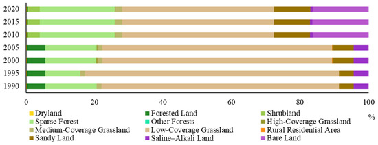
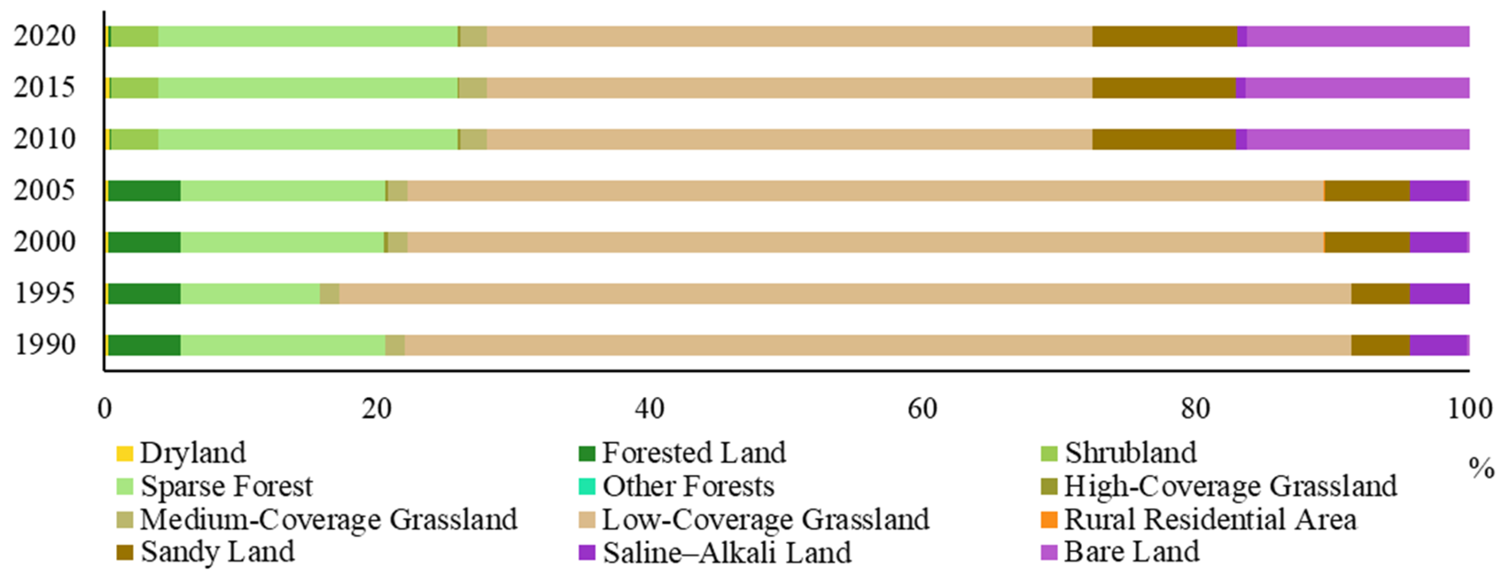
Based on land use data for seven time points from 1990 to 2020, this study analyzed the proportional changes in and spatiotemporal characteristics of twelve land cover types dominated by vegetation. Overall, the land cover structure in the study area has undergone a significant transformation over the past three decades (Figure 3).

From a temporal perspective, the structure of the vegetation types underwent a pronounced shift around 2010 (Figure 3). The transition matrix analysis further indicates that the most substantial conversion occurred during 2005–2010, when large areas of forested land were converted to shrubland, accompanied by smaller conversions into sparse forest and low-coverage grassland. Between 1990 and 2005, low-coverage grassland and sparse forest dominated the land cover composition, accounting for more than 80% of the total area. During this period, forested land remained relatively stable at approximately 5%, medium-coverage grassland occupied approximately 1.4%, and saline-alkali land maintained a proportion of approximately 4.3%. Sandy land showed a slight increase, particularly during 1995–2000. High-coverage grasslands first appeared after 2000, albeit with an extremely small proportion of roughly 0.2%. A substantial transformation occurred after 2010. The proportion of sparse forests increased from approximately 14% to approximately 21%. Shrubland appeared for the first time and stabilized at approximately 3.5%, whereas bare land remained steady at approximately 16.34%; however, during the period from 1990 to 2010, bare land accounted for only 0.15% of the study area. In contrast, forested land and low-coverage grasslands experienced pronounced declines. The proportions of high-coverage and medium-coverage grasslands remained largely unchanged, with only minor fluctuations.

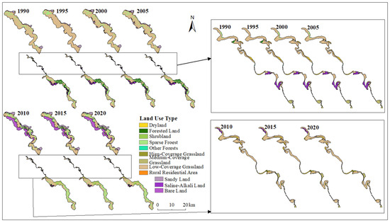
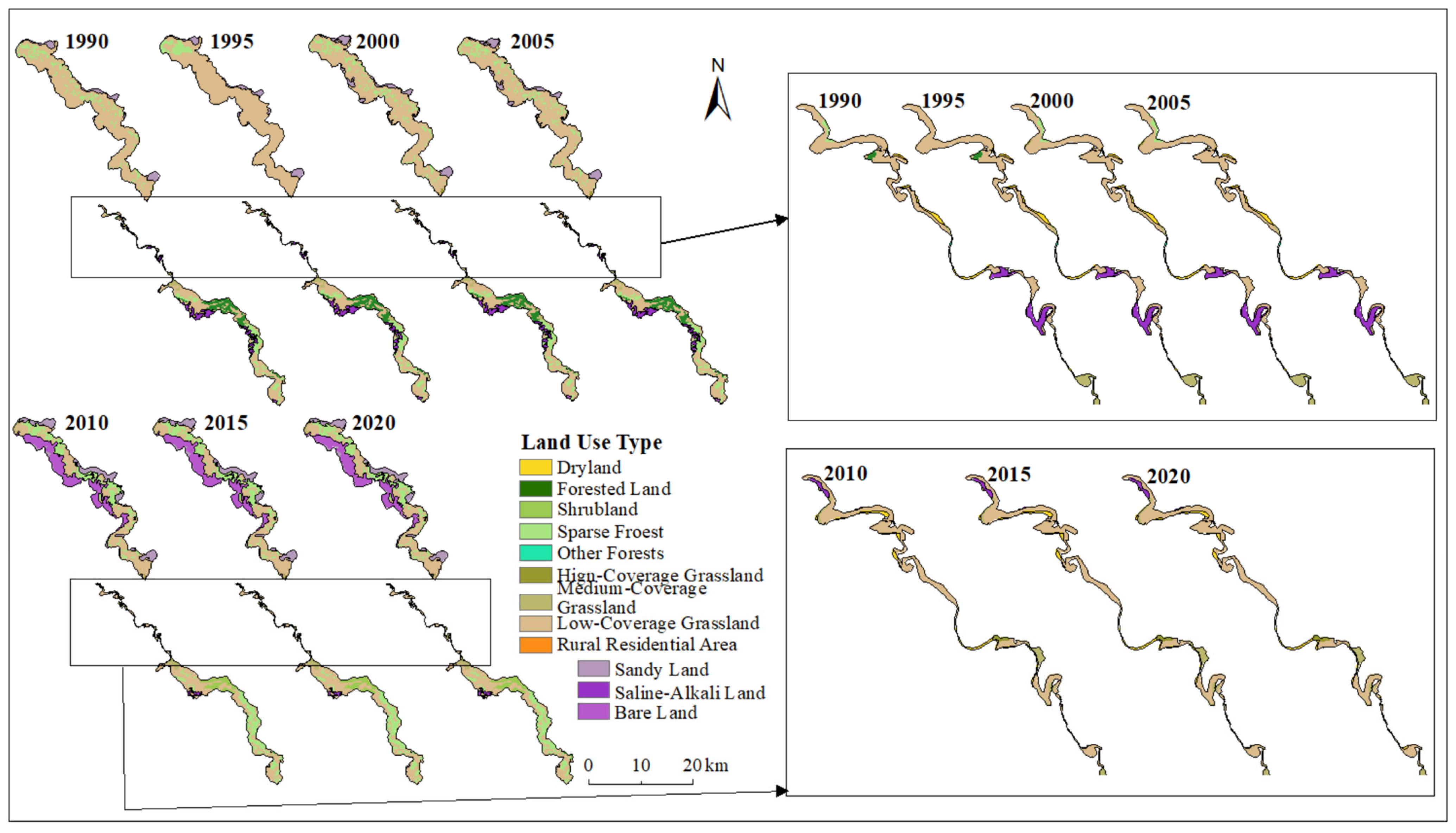
From the perspective of spatial differentiation, sparse forests and low-coverage grasslands consistently dominated the region throughout the entire study period, and all land cover types exhibited pronounced spatiotemporal heterogeneity (Figure 4). Significant spatial changes occurred between 1990 and 2020, including the rapid expansion of saline-alkali land in the north after 2010, which continued to shift southward. Additionally, the bare land in the central-southern area shrank after 2010 and was gradually replaced by other land types. Forest land types (including forested land, sparse forest, and other forest types) remained concentrated in the central-southern region, and after 2010, sparse forests and other forests showed an increasing trend of forming contiguous patches with forested land. Among grasslands, high-coverage grassland expanded southward, medium-coverage grassland slightly expanded in the central-southern part, while low-coverage grassland and dry land markedly decreased due to the northward expansion of saline-alkali land. Sandy land and rural settlements showed minimal spatial variations.

Based on multi-temporal LULC datasets from 1990 to 2020, the spatiotemporal transitions of land cover types within the study area (totaling 253.95 km²) were systematically analyzed.

Forested land remained largely stable between 1990 and 2005, with only small portions converted to sparse forest or grassland, and generally maintained an area above 13 km². However, a substantial shift occurred between 2005 and 2010, during which large areas of forest were converted to shrubland, accompanied by smaller conversions into sparse forests and low-coverage grasslands. After 2010, the rate of forest conversion gradually decreased. Over the entire 1990–2020 period, 7.33 km² of forested land transitioned to shrubland and 1.78 km² to sparse forest. Shrubland occupied only a limited area in 1990 but expanded steadily over time, particularly during 2005–2010 due to the influx of former forested land; a small portion of low-coverage grassland also shifted to shrubland. Sparse forest exhibited pronounced fluctuations throughout the study period: its area was 37.96 km² in 1990 and slightly decreased by 2020. Frequent two-way transitions occurred between sparse forests and low-coverage grasslands. For example, in 1990, 16.22 km² of sparse forest was converted to low-coverage grassland, whereas in subsequent years, some grassland areas reverted to sparse forest. A small amount of sparse forest also shifted to bare land during this period.

Among the grassland types, high-coverage grassland remained limited in area and showed minimal change, whereas medium-coverage grassland increased slightly from 3.78 km² in 1990 to 2020, primarily through exchanges with low-coverage grassland. Low-coverage grassland peaked in 1995 at 188.08 km² and slightly declined by 2020, but it continued to dominate the landscape thereafter. Significant transitions occurred between low-coverage grasslands and sandy, saline-alkali, and bare lands. From 1990 to 2020, 15.65 km² of low-coverage grassland was converted to sandy land and 0.47 km² was converted to saline-alkali land.

Non-vegetated categories, such as sandy, saline-alkali, and bare land, remained relatively stable overall but exhibited frequent exchanges with low-coverage grasslands. Sandy land expanded, particularly during the periods 1995–2000 and 2005–2010. Rural residential land showed minimal change throughout the study period.

3.2. Analysis of Vegetation’s Ecological Water Requirement in TRCZ

3.2.1. Overall Ecological Water Requirement in TRCZ

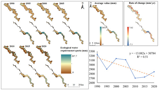
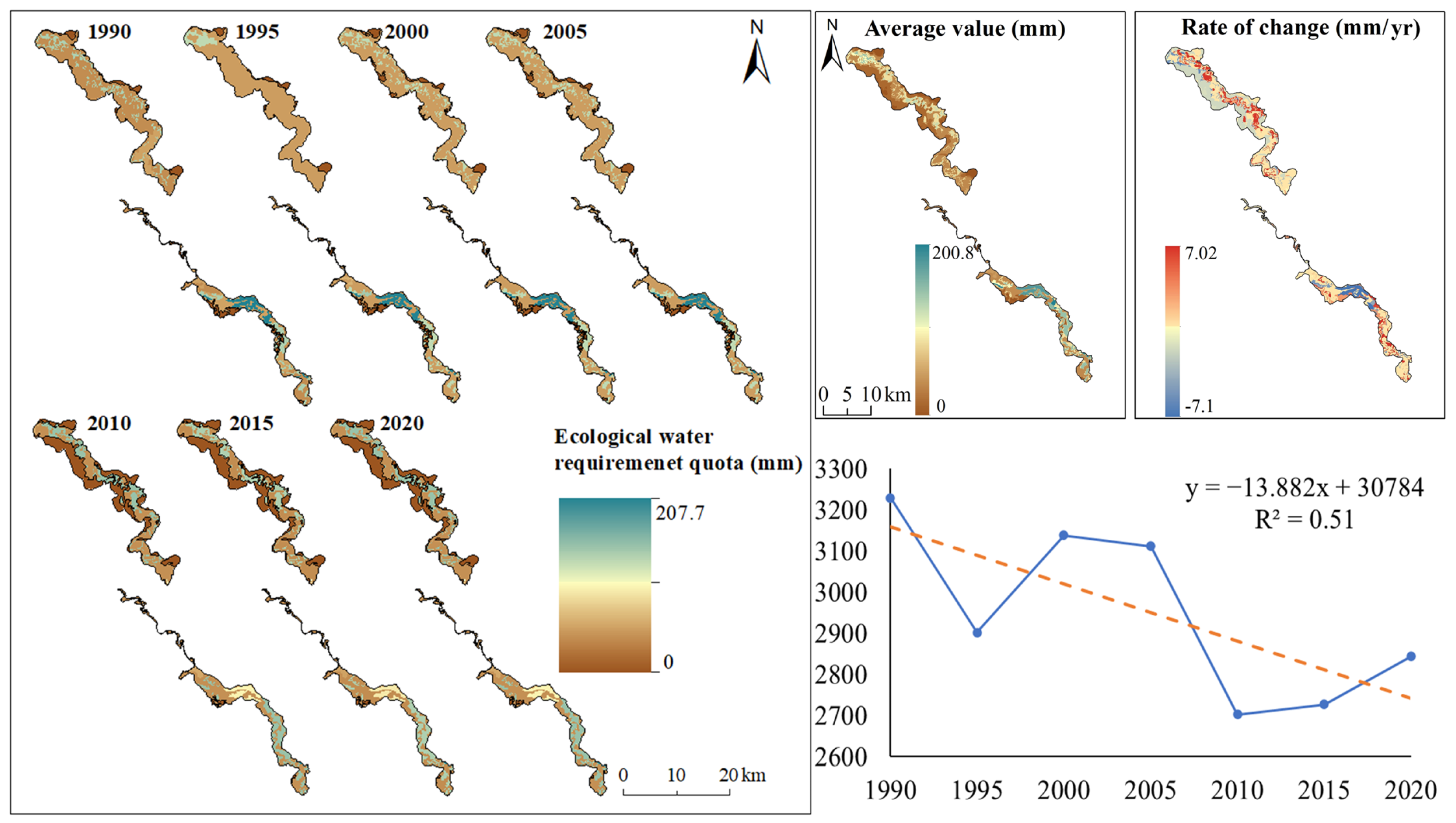
The multi-year average ecological water requirement quota in the study area was 2.95 × 10⁷ m³. The total ecological water requirement in the study area from 1990 to 2020 exhibited an overall declining trend with fluctuations, indicating a significant change in the aggregate water requirement of the regional ecosystem, with a change rate of 1.39 × 10⁵ m³/yr (Figure 5). Beginning at 3.23 × 10⁷ m³ in 1990, the ecological water requirement gradually decreased amid fluctuations, reaching a minimum of 2.70 × 10⁷ m³ in 2010. Although a slight rebound occurred thereafter, the total demand in 2020 (2.84 × 10⁷ m³) remained markedly lower than the initial level in 1990, representing an overall decrease of approximately 12% over the three decades. This temporal variation can be divided into two primary stages: the first stage (1990–2010) corresponds to a pronounced decline, with two notable minima observed in 1995 and 2010; the second stage (2010–2020) represents a period of low-level gradual recovery, during which water demand stabilized and fluctuated within a narrow range. This declining trend is strongly associated with shifts in vegetation cover type. Based on a comprehensive land use analysis of the earlier period, the shift in vegetation patterns around 2010 (with 7.33 km² of forested land converted to shrubland over the 30-year period) reduced the overall ecological water consumption in the study area. The slight subsequent increase in water demand after 2010 indicates that once vegetation conversion approached a new dynamic equilibrium, climatic changes (e.g., regional warming and moistening) and continued human activities (such as ecological water conveyance and vegetation restoration projects) continued to exert a combined influence on the total ecological water demand by affecting the water requirements per unit area of vegetation.

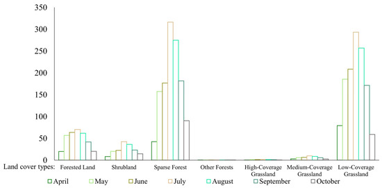
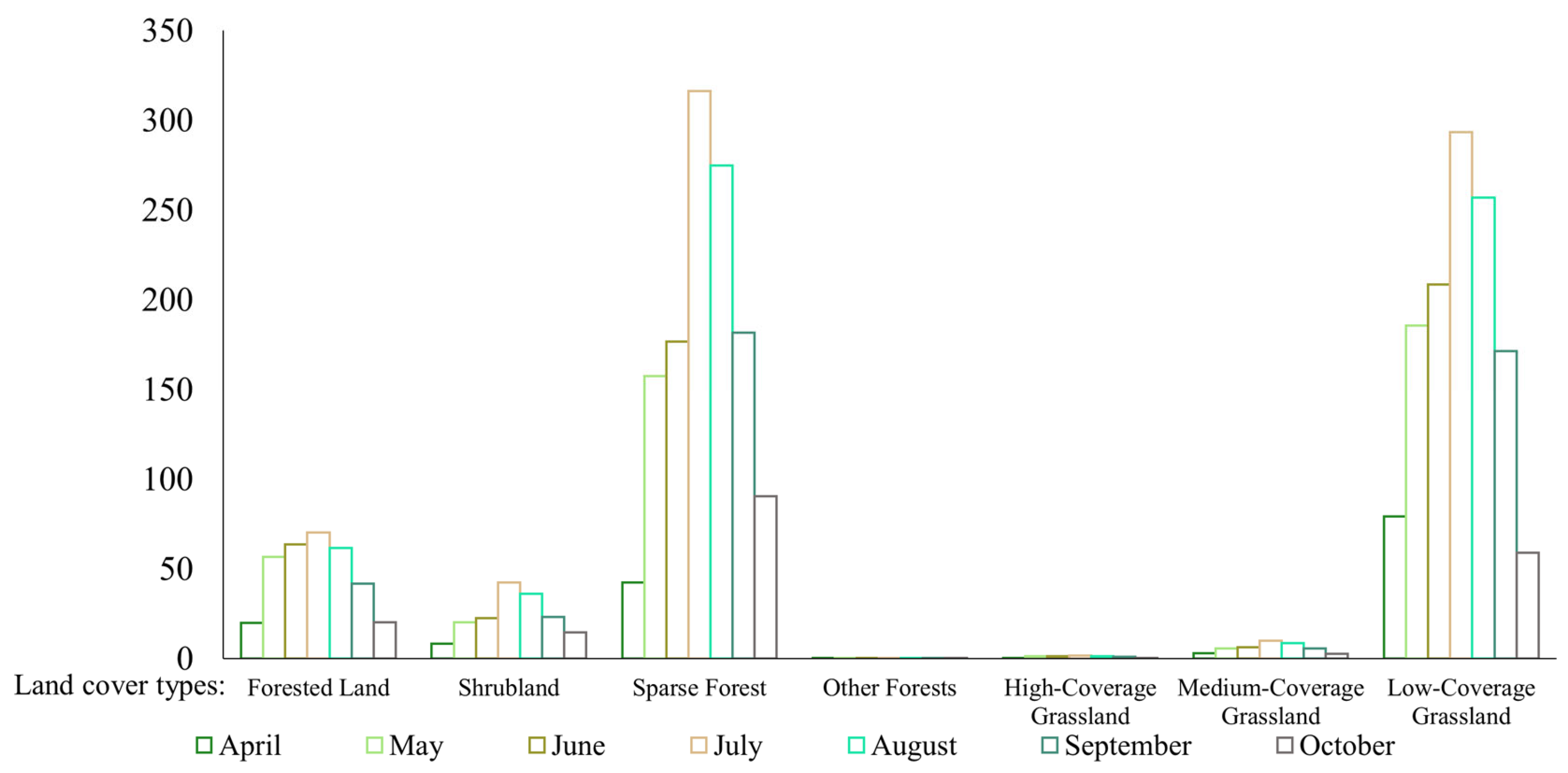
A detailed comparison of the monthly ecological water requirements in the study area from 1990 to 2020 revealed significant differences among vegetation types, influenced jointly by seasonal variation and human activities (Figure 6). Among the vegetation types, sparse forest consistently represented the largest water-consuming component, with a peak monthly demand of 4.09 × 10⁶ m³ in July 2020, markedly higher than that of other vegetation types. Low-coverage grassland ranked as the second-highest water-consuming component, reaching a peak of 3.68 × 10⁶ m³ in July 1995. Forested land was the third-largest water consumer prior to 2010, with a peak of 1.20 × 10⁶ m³ in July 1990; however, it declined sharply after 2010, dropping to only 3.33 × 10⁴ m³ in July 2020, representing a reduction of over 97%. Shrubland, emerging as a new vegetation type after 2010, exhibited a rapid increase in water demand, rising from 4.16 × 10⁵ m³ in July 2010 to 4.26 × 10⁵ m³ in July 2020, becoming a significant component of ecological water requirement. Seasonal dynamics indicated that all vegetation types exhibited a pronounced unimodal pattern, although the timing and magnitude of peak water demand differed. Sparse forest and grassland showed more prominent and prolonged peaks, lasting from May to September, sparse forest land and shrubland displayed relatively moderate peaks, concentrated between June and August. During the early growth stage (April), and differences in water demand among vegetation types were minor; however, by the mid-growth stage (July), sparse forest exhibited a significant increase in water demand.

Interannual comparisons indicate that vegetation water demand remained relatively stable between 2000 and 2005, but exhibited significant changes after 2010 (Figure 6). Forested land experienced a sharp decline in water demand, whereas shrubland and sparse forest showed increased demand. Notably, by 2020, the water demand of most vegetation types partially rebounded compared to 2015; for instance, sparse forest reached 4.09 × 10⁶ m³ in July 2020, slightly lower than 4.14 × 10⁶ m³ in July 2015, and low-coverage grassland increased from 2.31 × 10⁶ m³ to 2.27 × 10⁶ m³. This rebound trend may be attributed to enhanced evapotranspiration under climate change. From a monthly perspective, July represents the critical month with the highest ecological water requirement, during which all vegetation types reached their peak. April and October exhibited the lowest water demand, with all vegetation types consuming less than 1.00 × 10⁴ m³. The period from May to September constitutes the key ecological water requirement season, accounting for over 70% of the annual total (Figure 6). The ecological water requirement pattern in the study area has formed a configuration jointly dominated by sparse forest and low-coverage grassland (accounting for 81.84% of the total water requirement). Additionally, the influence of climate change is becoming increasingly evident, as reflected by the partial rebound of water demand in 2020. Long-term average ecological water requirement across vegetation types exhibited significant differences and consistent seasonal patterns. Sparse forest represents the primary water-consuming component in the region, reaching a peak of 7.73 × 10⁶ m³ during the mid-growth stage, substantially exceeding other vegetation types, indicating its extensive distribution and high transpiration rate. Low-coverage grassland and forested land also contributed significantly, with mid-growth stage demands of 7.22 × 10⁶ m³ and 1.74 × 10⁶ m³, respectively, establishing them as secondary water-consuming components.

In contrast, shrubland, medium-coverage grassland, and high-coverage grassland exhibited relatively limited water demand, while other forests had negligible demand. All vegetation types displayed a characteristic unimodal (“single-peak”) pattern of water consumption: demand was lowest during the early growth stage (all below 5.00 × 10⁴ m³), increased rapidly during the development stage, peaked in the mid-growth stage, and declined thereafter to levels similar to the early stage (Figure 6). Consequently, the mid-growth stage represents the period of most concentrated water demand and is critical for water resource management. Overall, water demand management for sparse forest, low-coverage grassland, and forested land during the mid-growth stage should be prioritized in regional water allocation strategies for the study area.

3.2.2. Ecological Water Requirement of Vegetation Across Different Growing-Season Periods in TRCZ

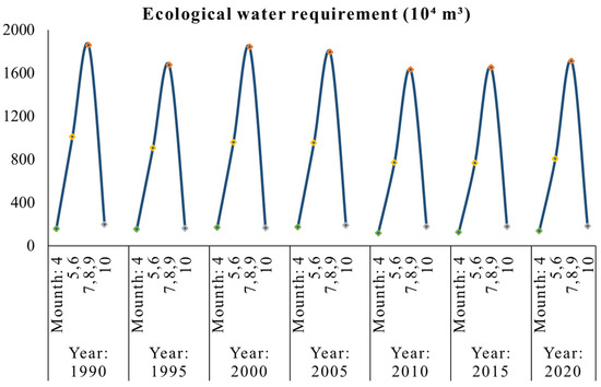
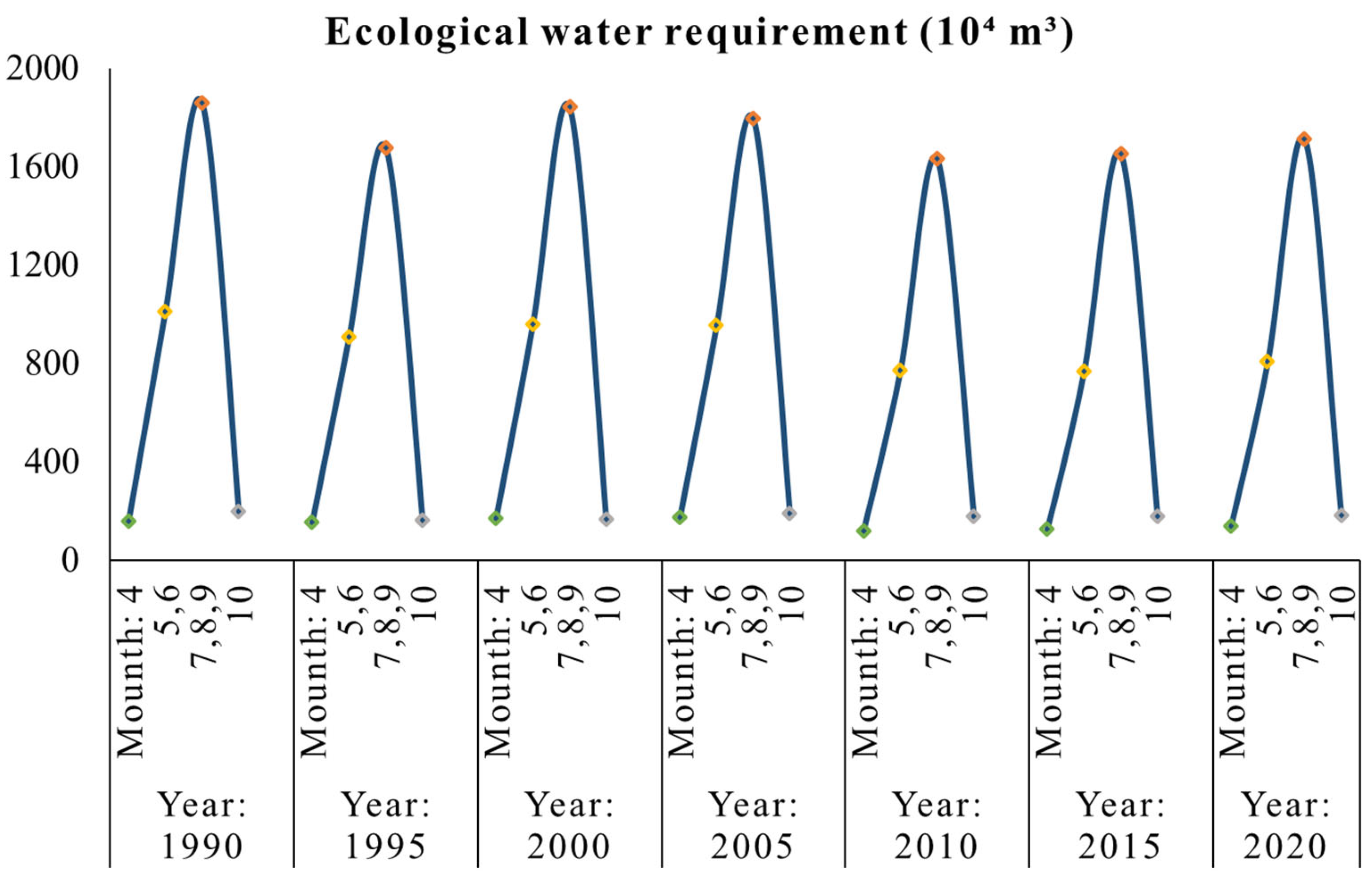
Based on four defined vegetation growth stages (initial growth: April; development stage: May–June; mid-growth: July–September; late-growth: October), this study analyzed the spatial-temporal dynamics of ecological water requirement quotas in the study area (Figure 7).

During the initial growth stage, the multi-year average water demand quota was the lowest (12.6 mm). The total ecological water requirement for this stage showed a declining trend from 1990 to 2020, with a linear slope of approximately −0.68 × 10⁴ m³/yr (Figure 7).

The development stage showed consistently higher water demand quotas in the southeastern region compared to the northwest over the 30-year period, with a multi-year average of 34.6 mm. From 1990 to 2005, the central-southeastern region maintained a high average quota of 76.6 mm, which dropped sharply to 24.4 mm after 2005. Concurrently, the demand centroid shifted toward the central-northwestern area, where the quota increased from 13.8 mm (1990) to 37.4 mm (2020) (Figure 7). Supporting data indicate that the total ecological water requirement during this stage decreased from approximately 1.01 × 10⁷ m³ in 1990 to 8.09 × 10⁶ m³ in 2020, with a linear slope of approximately −6.74 × 10⁴ m³/yr, reflecting a significant and steady reduction in water demand over time (Figure 7).

During the mid-growth stage, the multi-year average water demand quota peaked at 42.0 mm. Although southeastern quotas were generally higher, a spatial redistribution occurred after 2005, with a slight decrease in the southeast and an increase in the northwest. The average quota declined by 8.1% from 43.5 mm (pre-2005) to 39.9 mm (post-2005), with minimal temporal variation. The demand centroid also shifted northward during this period (Figure 7). Correspondingly, the total ecological water requirement in this stage decreased from 1.86 × 10⁷ m³ in 1990 to 1.71 × 10⁷ m³ in 2020, with a linear slope of approximately −5.02 × 10⁴ m³/yr, indicating a persistent, albeit slightly slower, declining trend compared to the development stage.

In the late-growth stage, the multi-year average quota was 14.3 mm, second only to the initial stage. The total water requirement for this stage exhibited a very gentle positive trend with a slope of approximately 0.28 × 10⁴ m³/yr, suggesting relative stability over the studied decades.

3.3. Analysis of Ecological Water Requirements of Different Vegetation Types Across Growing Season Periods in TRCZ

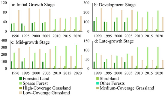
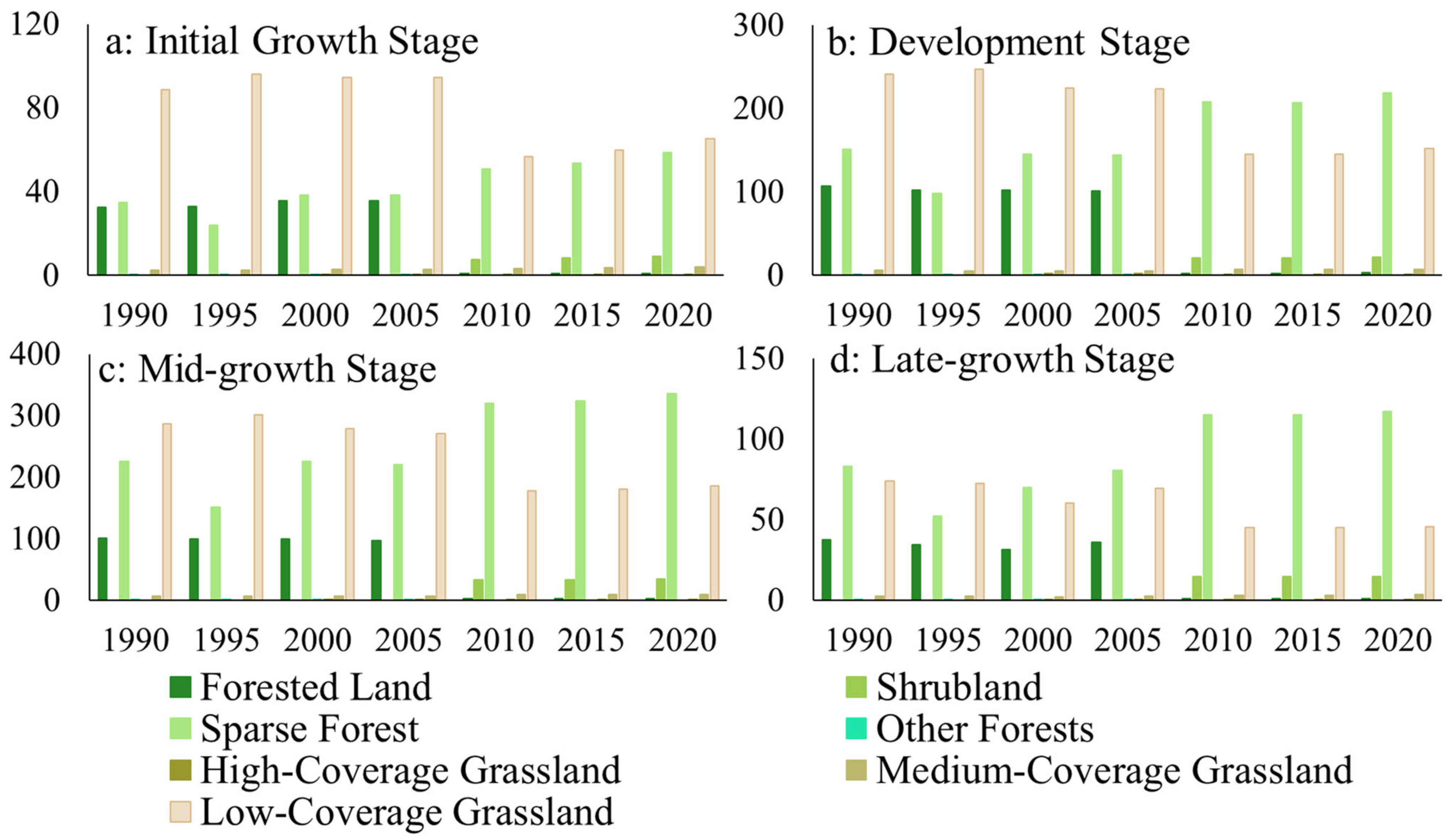
Based on seven temporal snapshots from 1990 to 2020, a systematic analysis was conducted on the ecological water requirement of the major vegetation types (forested land, shrubland, sparse forest, other forests, high-coverage grassland, medium-coverage grassland, and low-coverage grassland) across four growth stages (initial, development, mid, and late). In terms of total ecological water requirements, the study area exhibited a relatively stable trend over the 30-year period (Figure 6).

Taking the mid-growth stage as an example, the total ecological water requirement was 6.21 × 10⁶ m³ in 1990 and approximately 5.71 × 10⁶ m³ in 2020, indicating relatively little change in total demand (Figure 8). However, the vegetation composition shifted from a distribution pattern dominated by forested land, sparse forest, and low-coverage grassland to one dominated by sparse forest, shrubland, and low-coverage grassland. Among vegetation types, sparse forest and low-coverage grassland exhibited significantly higher ecological water requirements than other types. For instance, in 1990, the mid-growth stage water demand for sparse forest was 2.25 × 10⁶ m³ and for low-coverage grassland was 2.87 × 10⁶ m³. The water demand of forested land and shrubland was relatively low, and that of other woodland and high-coverage grassland was minimal, often below 1.00 × 10⁴ m³, primarily due to their small spatial extent (Figure 8). Temporally, from 1990 to 2005, the water demand of all vegetation types remained relatively stable with minor fluctuations across growth stages. After 2010, the demand of sparse forest and grasslands increased; for example, in the 2020 mid-growth stage, sparse forest reached 3.36 × 10⁶ m³ and low-coverage grassland reached 1.87 × 10⁶ m³, showing notable increases compared with earlier periods. Across growth stages, all vegetation types exhibited a “low-high-low” trend, with lower water demand in the initial and late-growth stages and peak demand during the development and mid-growth stages.

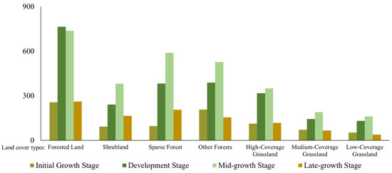
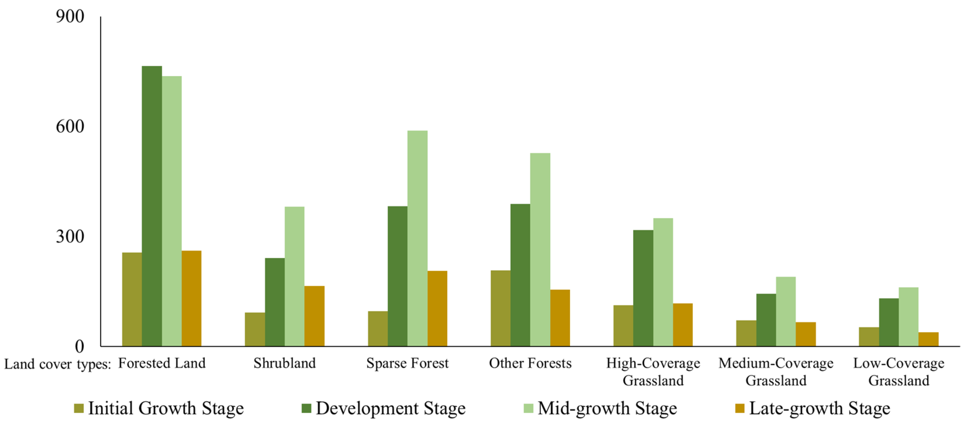
Significant differences exist in the unit area ecological water requirement among different vegetation types. Based on the data, forested land exhibits the highest unit area ecological water requirement throughout the whole growth stage (2018.66 m³/ha), which is 2.29 times that of shrubland (880.32 m³/ha) and 5.22 times that of low-coverage grassland (386.73 m³/ha) (Figure 9). Following forested land, other forests and sparse forest show similar whole-stage values at 1278.59 m³/ha and 1273.50 m³/ha respectively. The unit area ecological water requirement of high-coverage grassland (897.87 m³/ha) is notably close to that of shrubland, with a difference of only 17.55 m³/ha. Across growth stages, forested land maintains the highest unit area ecological water requirement in each period. Its peak value reaches 764.40 m³/ha in the development stage. In the mid-growth stage, sparse forest shows the second highest requirement (588.03 m³/ha), which is 79.8% of the value for forested land in the same period (Figure 9). The peak unit area ecological water requirement for shrubland occurs in the mid-growth stage (381.37 m³/ha), while for high-coverage grassland it occurs in the development stage (317.04 m³/ha). Low-coverage grassland consistently exhibits the lowest unit area ecological water requirement across all stages, with its peak value being 132.13 m³/ha in the development stage. The contribution of each growth stage to the total unit area ecological water requirement varies. For forested land, the development and mid-growth stages together account for 74.4% of its total. In contrast, for low-coverage grassland, the same two stages contribute 75.9% of the total.

3.4. Simulation Analysis of Water Yield Service Function in TRCZ Based on the InVEST Model

Over the past 30 years, the TRCZ has been subject to the dual influences of climate change and human activity, resulting in significant changes in the spatial distribution of its underlying surface patterns. Building on the analysis of the spatiotemporal heterogeneity of ecological water requirements, this study further aimed to assess the current status of soil and water conservation functions. To achieve this, we employed the water yield module of the InVEST model to simulate the water yield service function in the study area from 1990 to 2020, and analyzed its spatiotemporal heterogeneity.

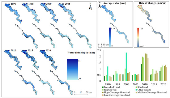
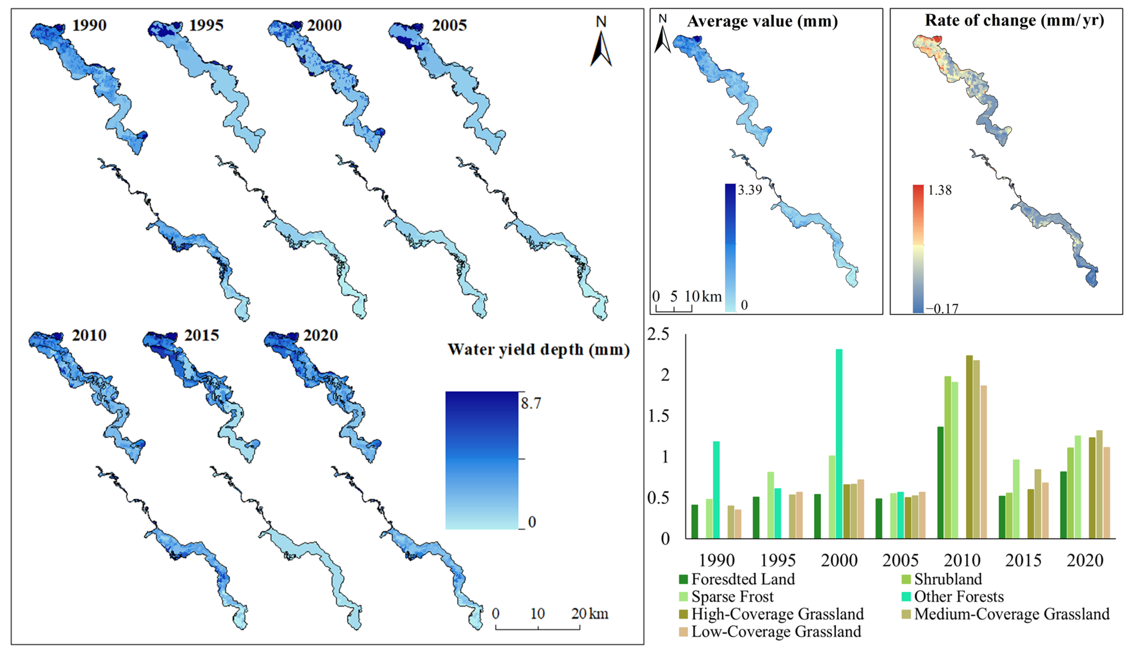
The total water yield across the region amounts to 2.40 × 10⁵ m³, and the mean water yield depth increases at a rate of 0.034 mm/yr. Despite noticeable interannual variability, the long-term upward trend in the regional water yield function remains weak. Distinct differences emerged among vegetation types in the unit area water yield function (Figure 10). Forested land and other forests consistently appeared in the high-value range, with forested land reaching a mean water yield depth of 1.909 mm in 2010, the highest among all vegetation types, underscoring the superior water yield performance of forest ecosystems. Grasslands exhibited considerably lower water yield depths, with low-coverage grasslands showing the lowest mean value (0.007 mm). Except for other forests, most vegetation types displayed positive trends. Sparse forests recorded the strongest increase among forest types (0.033 mm/yr), whereas high-coverage grasslands showed the highest growth rate within grasslands (0.035 mm/yr). Regarding total water yield, low-coverage grassland overwhelmingly dominates. Its unit area water yield function is modest, yet its extensive distribution results in a multi-year average water yield of 7.90 × 10⁴ m³—far exceeding all other vegetation types (Figure 10). Sparse forests are another significant contributor, with 3.48 × 10⁴ m³. In contrast, forested land, other grassland types, and the remaining vegetation categories made comparatively minor contributions. Overall, the findings demonstrate that broadly distributed low-coverage ecosystems constitute the principal carriers of water yield services in the study region, emphasizing their indispensable role in maintaining the regional water balance.

3.5. Drivers of Ecological Water Requirement in the TRCZ: Random Forest Analysis

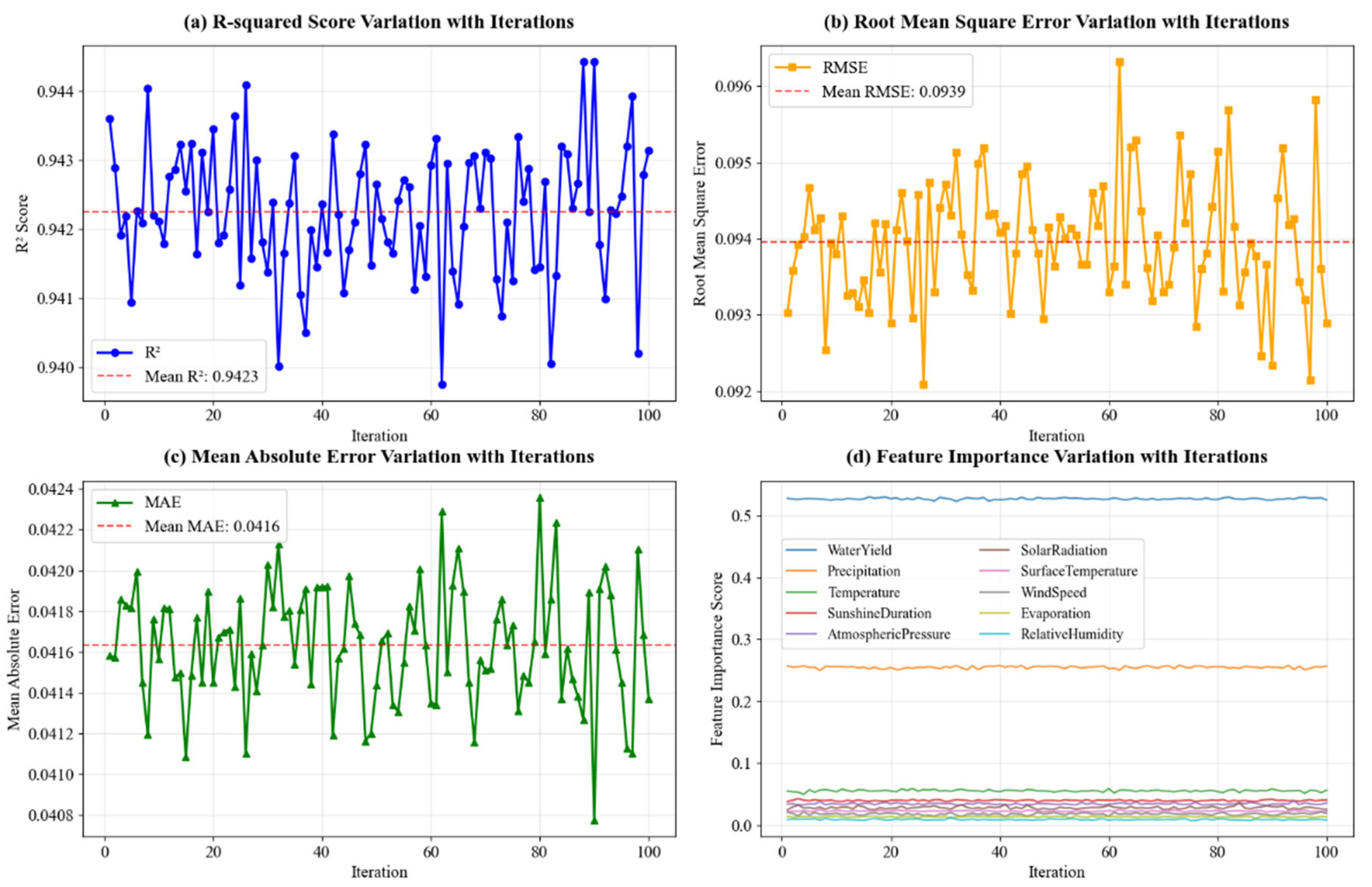
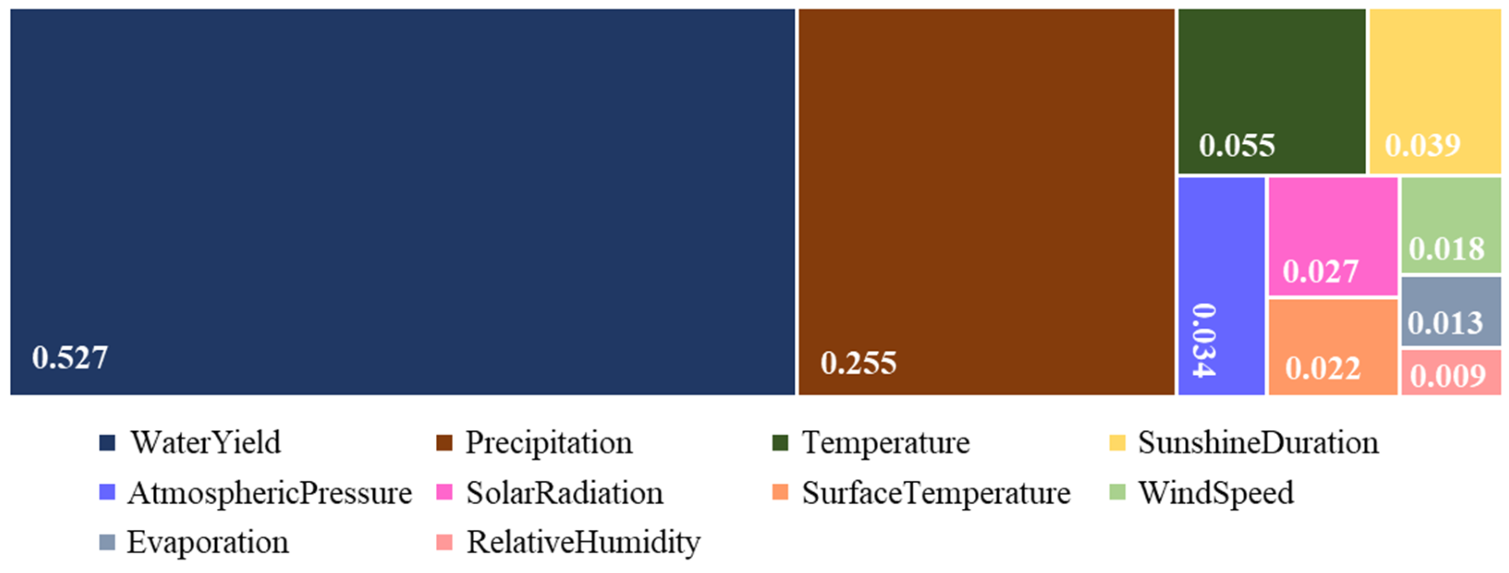
To identify the dominant drivers of ecological water requirement quotas in the TRCZ, Random Forest (RF) regression was implemented using nine meteorological variables (precipitation, temperature, sunshine duration, atmospheric pressure, solar radiation, surface temperature, wind speed, evaporation, and relative humidity) together with the InVEST derived water yield as candidate predictors. Model evaluation indicated strong predictive performance (R² = 0.942; RMSE = 0.094; MAE = 0.042). Feature-importance analysis showed that water yield was the most influential predictor (importance = 0.527), followed by precipitation (0.255) and temperature (0.055), whereas the remaining meteorological variables exhibited comparatively lower importance. This integrated analysis is intended to elucidate the response relationships among ecological water requirements, regional water yield functions, and principal environmental drivers, thereby providing robust quantitative evidence to inform mechanistic understanding.

The results reveal that the ecological water requirement in the TRCZ is strongly regulated by land cover structure and vegetation composition, which in turn shape regional ecosystem service functions, particularly water yield and soil–water conservation. From 1990 to 2020, the total ecological water requirement exhibited an overall declining trend with fluctuations, decreasing by approximately 12%, while distinct phase transitions occurred around 2010. This temporal inflection coincides with pronounced land use transformations, especially the conversion of forested land to shrubland and the restructuring of grassland types, indicating that vegetation pattern adjustment is a primary driver of ecological water requirement dynamics. Sparse forests and low-coverage grasslands jointly dominate the regional ecological water requirements, accounting for 81.84% of the total water demand. This dominance arises not from exceptionally high unit-area water requirements, but from their extensive spatial distribution. In contrast, forested land exhibited the highest unit area ecological water requirement (2018.66 m³/ha) but contributed relatively little to the total demand owing to its limited area. This structural mismatch highlights a key ecohydrological principle: regional ecological water demand is primarily governed by landscape-scale vegetation composition rather than by the water demand intensity of individual vegetation types, a pattern that is widely observed in arid and semi-arid river basins [12,29]. Seasonally, the ecological water requirement displayed a consistent unimodal pattern across vegetation types, with the mid-growth stage (July–September) representing the critical period, contributing over 70% of the annual ecological water requirement. This aligns with the period of peak evapotranspiration and vegetation physiological activity. Sparse forests show the most pronounced mid-growth water demand peak, reflecting their high transpiration capacity and deep rooting systems, which enhance access to groundwater and soil moisture. Similar seasonal dominance of woody vegetation in regulating ecosystem water fluxes has been reported in other inland river/lake systems of northwestern China [13,14].

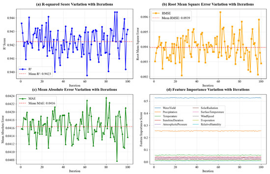
In this study, the RF model was applied to quantify the key drivers of ecological water demand quota through 100 iterative simulations and to elucidate their intrinsic linkages with regional water yield processes. The model evaluation results demonstrated excellent robustness and suitability. On average, the model achieved an R² of 0.942, with RMSE and MAE values of 0.094 and 0.042, respectively (Figure 11). These performance metrics confirm the model’s strong capability in capturing the nonlinear interactions between ecological water requirements and environmental variables, thereby providing a reliable basis for identifying the dominant driving factors.

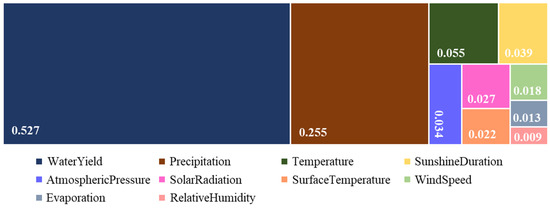
The feature importance analysis revealed a distinct hierarchical pattern of driving factors. Among them, water yield exhibited the highest importance score (0.527), substantially exceeding all other variables (Figure 12). Precipitation ranked second with an importance score of 0.255, and together, these two variables constitute the water yield dimension that predominantly governs ecological water requirements. Notably, temperature emerged as the third most important driver (0.055), indicating its non-negligible role in indirectly shaping ecological water requirements through its regulation of evapotranspiration processes. In contrast, energy-related variables, such as sunshine duration (0.039) and atmospheric pressure (0.034), showed relatively limited contributions, whereas factors, including land surface temperature and wind speed, exerted even lower impacts (Figure 12). This hierarchical structure suggests that the establishment of ecological water quotas is primarily constrained by water yield conditions, with energy factors playing a secondary role in this process. A strong coupling relationship exists between the ecological water requirements and the water yield function. When water yield is abundant, key ecohydrological processes can be sustained, and the threshold of ecological water requirements tends to increase accordingly. Conversely, insufficient water yield directly limits the extent to which ecological water requirements can be satisfied. This relationship is not unidirectional but involves a dynamic feedback mechanism: adequate ecological water allocation supports vegetation functioning and enhances infiltration processes, which in turn promotes long-term water yield function, whereas persistent ecological water deficits may lead to ecosystem degradation and ultimately weaken water yield function.

The water yield function highlights the direct constraint imposed by the amount of water actually available for ecosystem use, underscoring its foundational role in determining ecological water requirements. The importance score of precipitation was approximately half that of water yield (Figure 12), indicating that atmospheric water inputs must undergo surface regulation and runoff generation processes before becoming an effective water yield. This attenuated “precipitation-water yield” chain reveals the critical regulatory role of terrestrial ecosystems within the hydrological cycle. Although the contribution of temperature was comparatively lower, its position as the third most influential factor was scientifically meaningful. Temperature influences ecological water requirements through two pathways: directly by intensifying evapotranspiration and increasing ecosystem water demand, and indirectly by modulating snow and ice melt as well as soil freeze–thaw processes, thereby reshaping water yield patterns. These dual effects operate simultaneously on both the supply and demand sides of the water balance. This hierarchical driving structure demonstrates that ecological water requirements are not solely constrained by the initial availability of water resources (precipitation), but depend more critically on the ecosystem’s function to regulate and transform water inputs (water yield function), while also being dynamically modulated by energy conditions (temperature). Accordingly, ecological water resource management should prioritize enhancing water yield functions by optimizing landscape patterns to strengthen hydrological regulation. Meanwhile, management strategies must account for the potential pressures imposed by rising temperatures under climate warming on the equilibrium between water yield and demand, thereby enabling the development of adaptive and resilient management frameworks.

4. Discussion

4.1. Interpretation of the 2005–2010 Land-Cover Transition and Drivers of Ecological Water Requirement in the TRCZ

The results revealed a distinct land-cover reorganization during 2005–2010, especially the conversion of forested land to shrubland and associated restructuring among woody and grassland classes. Because this transition coincides with the major inflection in the total ecological water requirement trajectory (minimum around 2010), the discussion below first interprets the likely mechanisms behind the 2005–2010 land-cover shift and then explains how hydrological supply and climate jointly constrain ecological water requirement in a coupled “supply–demand” framework. The land-cover transition matrix indicates that forested land was relatively stable up to 2005, but experienced its most substantial conversion during 2005–2010 when large areas were converted to shrubland, with additional exchanges among sparse forest and low-coverage grassland classes. A key reason why this shift appears abrupt is that the land-cover classes are defined by canopy/cover thresholds (e.g., forested land vs. sparse forest), so gradual changes in canopy density or vertical structure can translate into step-like class transitions between mapping years once thresholds are crossed. Ecologically, the shift is consistent with a structural adjustment of downstream woody vegetation under strong water limitation: under restricted and spatially heterogeneous water availability, dense riparian tree cover may not be sustainable everywhere, while shrubs and sparse woody cover can persist under lower or more variable water supply. In an arid downstream inland river basin, water availability is the primary constraint on vegetation structure; accordingly, we interpret hydrological conditions (surface flow continuity, groundwater recharge, and soil moisture availability) as the dominant trigger shaping the 2005–2010 land-cover adjustment. The driver analysis (reported in Section 3.5) supports this interpretation by identifying water yield and precipitation as the leading predictors of ecological water requirement quotas, with temperature as a secondary influence. At the same time, land-cover change modifies the demand side of the water balance by altering evapotranspiration and thus ecological water requirement; this can feed back to hydrological functioning (e.g., via changes in evapotranspiration and infiltration). Therefore, hydrology and land cover are coupled, but the results indicate a primarily supply-constrained system in which hydrological variability initiates land-cover adjustment and the resulting vegetation restructuring reinforces the observed ecological water requirement dynamics.

The results reveal four robust patterns that should be clarified before proposing management recommendations. First, land-cover composition remained relatively stable prior to 2005 but underwent a pronounced reorganization during 2005–2010, notably the conversion of forested land to shrubland and restructuring among woody and grassland classes. Second, total ecological water requirement exhibited a two-stage temporal trajectory, declining from 1990 to an inflection/minimum around 2010, followed by a modest rebound during 2010–2020. Third, ecological water demand showed strong seasonal concentration, with the mid-growth stage (July–September) accounting for >70% of annual ecological water requirement. Fourth, driver analysis indicates that ecological water requirement is primarily constrained by water yield and precipitation, with temperature acting as a secondary modifier through evaporative demand. Taken together, these patterns indicate a supply-constrained downstream arid system in which vegetation composition shapes demand and hydrological availability limits achievable ecological quotas; therefore, recommendations should prioritize seasonally targeted allocation and land-cover protection/optimization aligned with these constraints. The TRCZ has been influenced not only by climate variability but also by human interventions, particularly ecological water conveyance since 2000 and associated restoration initiatives, which plausibly contributed to vegetation restructuring and localized recovery near the river corridor; however, because spatially explicit, time-resolved records of vegetation management practices (e.g., planting/harvesting, grazing regulation, land-use enforcement, or site-level restoration actions) were not available consistently for 1990–2020, our analysis does not directly quantify management intensity or attribute specific land-cover transitions (including the 2005–2010 shift) to discrete management changes, and management is therefore discussed as a plausible contributing context while the quantified driver analysis focuses on hydrological supply and climatic controls captured by water yield and meteorological variables.

4.2. Recommendations for Sustainable Management of Water and Soil Resources in TRCZ

The recommendations below are derived directly from the clarified patterns synthesized at the end of Section 4.1: (i) the 2005–2010 land-cover transition and associated vegetation restructuring; (ii) the two-stage temporal dynamics of total ecological water requirement with an inflection/minimum around 2010 and partial rebound thereafter; (iii) the strong seasonal concentration of ecological water demand during July–September; and (iv) the dominant control of water yield and precipitation (with temperature as a secondary modifier). Accordingly, sustainable management in the TRCZ should shift from generalized interventions toward pattern-based ecological water allocation and land-cover protection/optimization, using ecological water requirement as a quantitative bridge linking vegetation composition, hydrological regulation, and ecosystem services. Because this study does not include spatially explicit vegetation-management datasets, the recommendations emphasize water-allocation timing, seasonal priorities, and land-cover protection targets rather than prescribing specific site-level management operations.

(1)

The dominance of sparse forests and low-coverage grasslands in both ecological water requirements and total water yield highlights their irreplaceable role in maintaining the regional water balance. Although forested land exhibits superior unit-area water yield and ecological water demand, its limited spatial extent constrains its contribution at the basin scale. Therefore, sustainable water and soil conservation strategies should prioritize the stability and functional optimization of widely distributed vegetation types, rather than exclusively pursuing high-water-demand forest expansion, a principle increasingly emphasized in dryland restoration studies [15,30].

(2)

The pronounced seasonal concentration of ecological water demand during the mid-growth stage underscores the importance of synchronizing water management with the vegetation phenology. Because over 70% of the annual ecological water requirement occurs between July and September, water allocation strategies that ignore seasonal demand dynamics may lead to inefficient water use or ecological stress. Aligning ecological water yield with peak vegetation water demand is essential for enhancing water use efficiency and reducing non-productive losses such as excessive evaporation [31,32].

(3)

The strong influence of water yield on ecological water requirements emphasizes that soil and water conservation should focus on enhancing the landscape-scale hydrological regulation capacity. Improving soil infiltration, maintaining vegetation cover continuity, and preventing excessive land degradation are critical for sustaining water yields under limited precipitation conditions. In this context, low-coverage grasslands, despite their low unit-area water yield, function as extensive water-regulating matrices that support regional hydrological stability [33].

(4)

Vegetation-type differentiation in unit-area ecological water requirements suggests that water–soil conservation policies should be vegetation-specific rather than uniform. Forested land and sparse forest, with higher water demand intensity, require stable groundwater support and careful regulation to avoid overexploitation, while low-coverage grasslands should be managed to prevent further conversion to sandy or saline-alkali land, which was shown to be a significant transition pathway in the study area. Maintaining the integrity of grassland–shrubland mosaics is particularly important for preventing desertification and preserving soil structure in arid environments [34].

(5)

The partial rebound of ecological water requirement after 2010, likely driven by climate warming and increased evapotranspiration, indicates that future water and soil conservation strategies must be adaptive to climate change. Static management targets may become increasingly mismatched with dynamic ecohydrological conditions. Incorporating climate sensitivity into ecological water requirement assessments can enhance the resilience of water allocation and land management policies [35].

Overall, sustainable water and soil conservation in TRCZ should emphasize maintaining functional vegetation composition, enhancing water yield services through soil–vegetation regulation, and aligning ecological water allocation with seasonal and structural ecosystem demands. This approach moves beyond short-term engineering solutions toward long-term ecosystem resilience, providing a transferable framework for inland river basins in arid and semi-arid regions worldwide.

Although this study provides valuable insights into the driving mechanisms and management implications of ecological water requirements in the TRCZ, several limitations must be acknowledged. First, although the InVEST model employed for water yield estimation is widely applied, its uniform assumptions regarding hydrological processes—such as soil depth and plant available water content—may not fully capture local heterogeneity. Second, although the Random Forest model is robust, its “black-box” nature limits the explicit mechanistic interpretation of the complex nonlinear interactions among the driving factors. Third, the analysis primarily focused on natural environmental variables and did not quantitatively incorporate direct anthropogenic factors, such as water withdrawals and land management practices, which may affect the real-world applicability of the findings. Finally, the classification of vegetation types in this study remains relatively coarse; more refined ecological water requirement estimates for specific vegetation subtypes or functional types, such as grasslands dominated by different species or sparse forests of varying stand ages, require further research. Future efforts should integrate phenological observations and higher-resolution remote sensing data to develop more physiologically based and vegetation-specific estimation methods for ecological water requirements, thereby enhancing the targeting and timeliness of management measures. Future research could also help reduce these uncertainties by coupling process-based hydrological models, incorporating human activity data, and utilizing higher-resolution remote sensing information.

5. Conclusions

Understanding the interplay between land cover change, ecological water requirements, and their driving mechanisms is crucial for developing effective water allocation strategies in water-limited inland river basins. This study systematically investigated the spatiotemporal dynamics of land use and ecological water requirements in the TRCZ from 1990 to 2020. The principal conclusions are as follows:

(1)

The land cover structure underwent a significant transformation, particularly after 2010. The proportional area of sparse forest increased from approximately 14% to approximately 21%, whereas forested land experienced a pronounced decline. This transformation has profoundly influenced the regional ecosystem’s water demand structure.

(2)

The multi-year average ecological water requirement quota in the study area is 2.9 × 10⁷ m³. The total ecological water requirement exhibited a declining trend with fluctuations, accompanied by compositional changes. The overall ecological water requirement decreased at a rate of −1.39 × 10⁵ m³/yr over the 30-year period. This decline is strongly associated with vegetation pattern adjustments, specifically the conversion of forests to shrublands. Sparse forests remained the dominant water-consuming component throughout the study period.

(3)

Unit area ecological water requirements varied considerably among vegetation types and showed a widespread increasing trend. Forested land consistently exhibited the highest water consumption intensity, reaching 749.09 m³/ha during the mid growth stage in 2020. A gradual increase in the unit area water requirement was observed across most vegetation types, suggesting the influence of regional climatic background changes.

(4)

Water yield factors are the dominant drivers of ecological water requirements. The Random Forest model indicated that water yield (importance: 0.527) and (precipitation: 0.255) were the primary factors influencing the ecological water requirement, followed by (temperature: 0.055). This hierarchical structure demonstrates that ecological water requirements are primarily constrained by the water yield conditions.

Based on these findings, subsequent ecological restoration efforts should focus on establishing spatially differentiated ecological water conveyance schemes, strengthening ecological water allocation and process management, and optimizing landscape patterns to enhance water yield function. These measures will facilitate the transition from extensive water delivery to precise ecological rehabilitation in arid inland river basins.

References

- Deng, M.J.; Huang, Q.; Chang, J.X.; Huang, S.; Guo, A. Connotation, process and dimensionality of generalized ecological water conservancy. Adv. Water Sci. 2020, 31, 775–792. (In Chinese) [Google Scholar]
- Chen, Y.N.; Chen, Y.P.; Zhu, C.G.; Li, W.H. The concept and mode of ecosystem sustainable management in arid desert areas in northwest China. Acta Ecol. Sin. 2019, 39, 7410–7417. (In Chinese) [Google Scholar] [CrossRef] [Scilit]
- Ling, H.B.; Xu, H.L.; Guo, B.; Deng, X.; Zhang, P.; Wang, X. Regulating water disturbance for mitigating drought stress to conserve and restore a desert riparian forest ecosystem. J. Hydrol. 2019, 572, 659–670. [Google Scholar] [CrossRef] [Scilit]
- Li, F.J.; Han, F.; Ma, B.; Zhao, Y.; Chen, X.; Liu, X.; Wang, L.; Yin, L.; Lin, H. Response of vegetation evolution characteristics to ecological water transport in the lower reaches of Tarim River in recent 20 years. Pratacultural Sci. 2022, 39, 2578–2588. (In Chinese) [Google Scholar]
- Deng, M.J.; Zhou, H.Y.; Xu, H.L.; Ling, H.B.; Zhang, P. Research on the ecological operation in the lower reaches of Tarim River based on water conveyance. Sci. Sin. Technol. 2016, 46, 864–876. (In Chinese) [Google Scholar]
- Wang, H.; Li, X.; Xiao, J.; Ma, M. Evapotranspiration components and water use efficiency from desert to Alpine ecosystems in drylands. Agric. For. Meteorol. 2021, 298, 108283. [Google Scholar] [CrossRef] [Scilit]
- He, Y.; Min, Q.; Li, W.; Li, G.; Jin, L. Estimated forest ecological water requirements in the Jinghe watershed-Theory and case study. Front. Forest. China 2006, 1, 43–47. [Google Scholar] [CrossRef] [Scilit]
- Wang, H.; Li, X.; Xiao, J.; Ma, M.; Tan, J.; Wang, X.; Geng, L. Carbon fluxes across alpine, oasis, and desert ecosystems in northwestern China: The importance of water availability. Sci. Total Environ. 2019, 697, 133978. [Google Scholar] [CrossRef] [Scilit]
- Wang, H.B.; Ma, M.G. Impacts of climate change and anthropogenic activities on the ecological restoration of wetlands in the arid regions of China. Energies 2016, 9, 166. [Google Scholar] [CrossRef] [Scilit]
- Zhao, X.F.; Xu, H.L.; Zhang, P. Changes of lake area, groundwater level and vegetation under the influence of ecological water conveyance: A case study of the tail lake of Tarim River in China. Water 2022, 14, 1026. [Google Scholar] [CrossRef] [Scilit]
- Li, Z.; Liu, X.; Niu, T.; Kejia, D.; Zhou, Q.; Ma, T.; Gao, Y. Ecological restoration and its effects on a regional climate: The source region of the Yellow River, China. Environ. Sci. Technol. 2015, 49, 5897–5904. [Google Scholar] [CrossRef] [Scilit]
- Guo, W.; Jiao, A.; Wang, W.; Chen, C.; Ling, H.; Yan, J.; Chen, F. Change and driving factor analysis of eco-environment of typical lakes in arid areas. Water 2023, 15, 2107. [Google Scholar] [CrossRef] [Scilit]
- Yan, W.; Ma, X.; Liu, Y.; Qian, K.; Yang, X.; Li, J.; Wang, Y. Ecological assessment of terminal lake basins in central Asia under changing landscape patterns. Remote Sens. 2022, 14, 4842. [Google Scholar] [CrossRef] [Scilit]
- Zuo, T.F.; Chen, Y.N.; Ding, J.L. Research on vegetation coverage dynamics and prediction in the Taitema Lake region. Water 2022, 14, 725. [Google Scholar] [CrossRef] [Scilit]
- Ye, Z.; Chen, S.; Zhang, Q.; Liu, Y.; Zhou, H. Ecological water demand of Taitema Lake in the lower reaches of the Tarim River and the Cherchen River. Remote Sens. 2022, 14, 832. [Google Scholar] [CrossRef] [Scilit]
- Yang, C.-D.; Xu, M.; Kang, S.-C.; Fu, C.-S.; Zhang, W.; Hu, D.-D. Streamflow abrupt change and the driving factors in glacierized basins of Tarim basin, northwest China. Adv. Clim. Change Res. 2024, 15, 75–89. [Google Scholar] [CrossRef] [Scilit]
- Huang, M.; Mu, Z.; Zhao, S.; Yang, R. Ecological Water Requirement of Natural Vegetation in the Tarim River Basin Based on Multi-Source Data. Sustainability 2024, 16, 7034. [Google Scholar] [CrossRef] [Scilit]
- Deng, M.J.; Yang, P.N.; Zhou, H.Y.; Xu, H.L. Water Conversion and Strategy of Ecological Water Conveyance in the Lower Reaches of the Tarim River. Arid. Zone Res. 2017, 34, 717–726. (In Chinese) [Google Scholar]
- Huang, T.M.; Pang, Z.H. Changes in groundwater induced by water diversion in the Lower Tarim River, Xinjiang Uygur, NW China: Evidence from environmental isotopes and water chemistry. J. Hydrol. 2010, 387, 188–201. [Google Scholar] [CrossRef] [Scilit]
- Chen, Y.; Li, W.; Xu, C.; Ye, Z.; Chen, Y. Desert riparian vegetation and ground-water in the lower reaches of the Tarim River Basin. Environ. Earth Sci. 2015, 73, 547–558. [Google Scholar] [CrossRef] [Scilit]
- Kong, Z.J.; Deng, M.J.; Ling, H.B.; Wang, G.; Xu, S.; Wang, Z. Ecological security assessment and ecological restoration countermeasures in the dry-up area of the lower Tarim River. Arid. Zone Res. 2021, 38, 1128–1139. (In Chinese) [Google Scholar]
- Aili, A.; Xu, H.; Waheed, A.; Zhao, X.; Zhang, P. Unveiling the benefits of artificial ecological measures: Water conveyance improves the water quality of the Taitema Lake, northwestern China. Hydrology 2024, 11, 129. [Google Scholar] [CrossRef] [Scilit]
- Thevs, N.; Peng, H.; Rozi, A.; Zerbe, S.; Abdusalih, N. Water allocation and water consumption of irrigated agriculture and natural vegetation in the Aksu-Tarim River Basin, Xinjiang, China. J. Arid. Environ. 2015, 112, 87–97. [Google Scholar] [CrossRef] [Scilit]
- Quan, B. The Introduction to Land Use and Land Cover Change; China Science and Technology Press: Beijing, China, 2010. [Google Scholar]
- Suleiman, A.A.; Hoogenboom, G. Comparison of Priestley-Taylor and FAO-56 Penman-Monteith for daily reference evapotranspiration estimation in Georgia. J. Irrig. Drain. Eng. 2007, 133, 175–182. [Google Scholar] [CrossRef] [Scilit]
- Chen, Y.N. Ecological Protection and Sustainable Management in the Tarim River Basin of Xinjiang; Science Press: Beijing, China, 2015. (In Chinese) [Google Scholar]
- Natural Capital Alliance. InVEST User Guide. Available online: https://storage.googleapis.com/releases.naturalcapitalproject.org/invest-userguide/latest/en/index.html (accessed on 20 October 2025).
- Borup, D.; Christensen, B.J.; Muhlbach, N.S.; Nielsen, M.S. Targeting predictors in random forest regression. Int. J. Forecast. 2023, 39, 841–868. [Google Scholar] [CrossRef] [Scilit]
- Ling, H.; Zhang, P.; Guo, B.; Xu, H.; Ye, M.; Deng, X. Negative feedback adjustment challenges reconstruction study from tree rings: A study case of response of Populus euphratica to river discontinuous flow and ecological water conveyance. Sci. Total Environ. 2017, 574, 109–119. [Google Scholar] [CrossRef] [Scilit] [PubMed]
- Jiang, N.; Zhang, Q.; Zhang, S.; Zhao, X.; Cheng, H. Spatial and temporal evolutions of vegetation coverage in the Tarim River basin and their responses to phenology. Catena 2022, 217, 106489. [Google Scholar] [CrossRef] [Scilit]
- Song, J.; Betz, F.; Aishan, T.; Halik, Ü.; Abliz, A. Impact of water supply on the restoration of the severely damaged riparian plants along the Tarim River in Xinjiang, northwest China. Ecol. Indic. 2024, 158, 111570. [Google Scholar] [CrossRef] [Scilit]
- Huang, J.; Yu, H.; Dai, A.; Wei, Y.; Kang, L. Drylands face potential threat under 2 °C global warming target. Nat. Clim. Change 2017, 7, 417–422. [Google Scholar] [CrossRef] [Scilit]
- Zhang, Y.Q.; Peña-Arancibia, J.L.; McVicar, T.R.; Chiew, F.H.S.; Vaze, J.; Liu, C.; Lu, X.; Zheng, H.; Wang, Y.; Liu, Y.; et al. Multi-decadal trends in global terrestrial evapotranspiration and its components. Sci. Total Environ. 2016, 6, 19124. [Google Scholar] [CrossRef] [Scilit]
- Donohue, R.J.; Roderick, M.L.; McVicar, T.R. Roots, storms and soil pores: Incorporating key ecohydrological processes into Budyko’s hydrological model. J. Hydrol. 2012, 436–437, 35–50. [Google Scholar] [CrossRef] [Scilit]
- Yang, J.; Huang, X. The 30 m annual land cover dataset and its dynamics in China from 1990 to 2019. Earth Syst. Sci. Data 2021, 13, 3907–3925. [Google Scholar] [CrossRef] [Scilit]
Disclaimer/Publisher’s Note: The statements, opinions and data contained in all publications are solely those of the individual author(s) and contributor(s) and not of MDPI and/or the editor(s). MDPI and/or the editor(s) disclaim responsibility for any injury to people or property resulting from any ideas, methods, instructions or products referred to in the content. |
© 2026 by the authors. Licensee MDPI, Basel, Switzerland. This article is an open access article distributed under the terms and conditions of the Creative Commons Attribution (CC BY) license.