Seasonal Groundwater Trends and Predictions in Greenhouse Agriculture of Gyeongsangnam-Do Using Statistical and Deep Learning Models

Abstract

Seasonal groundwater (GW) pumping and climatic variability significantly impact the dynamics of greenhouse-dominated agricultural systems, yet quantitative evaluations at the local scale remain limited. This study explores non-parametric statistical and deep learning (DL) models for analyzing seasonal GW trends and predicting GW levels near greenhouse agriculture systems in Gyeongsangnam-do, South Korea. The modified Mann–Kendall (MK) test and Sen’s slope estimator were used to estimate long-term seasonal trends for the summer (wet season) and winter (dry season), based on monthly GW-level time series from six monitoring wells. Findings indicate that seasonal asymmetry is strong (winter trends have greater magnitudes and greater variability than summer trends), and that winter trends are negative (ranging from −0.45 to +1.70 m year⁻¹) and summer trends are positive (ranging from −0.02 to +0.31 m year⁻¹). At Jinju1 and Jinju4, statistically significant increasing trends were observed in both seasons (p < 0.05), but at other stations, weak or non-significant trends were observed due to short records or high variance. Long short-term memory (LSTM) and spatio-temporal graph neural network (STGNN) models were deployed and compared to predict at the GW level. The STGNN was found to be superior to LSTM in terms of R² (0.799–0.994) and reduced RMSE of up to 64.6, especially in winter, when spatially synchronized pumping is dominant in GW behavior. Despite advanced modeling, there is a serious concern about data limitations. Findings show that combining seasonal trend analysis with spatiotemporal modeling of DLs can significantly enhance knowledge and forecasting of GW dynamics in intensive greenhouse farming.

1. Introduction

Groundwater (GW) is a critical constituent of freshwater resources, indispensable for sustaining agricultural production, ecological stability, and water security in the region, especially amid increased water demand and a changing climate [1,2]. Increased agricultural irrigation, land-use transformation, and precipitation and evapotranspiration variability driven by a changing environment have led to extensive GW depletion, especially in areas with seasonal precipitation regimes [3,4]. GW is a strategic buffer in monsoon-dominated regions, such as South Korea, which experience extreme seasonal changes in precipitation, with heavy rainfall during the summer and extended dry spells during the winter and early spring [5,6]. Dependence on GW buffers has been observed in parts of East and South Asia affected by the monsoon, where seasonal abstraction is often greater than natural recharge during dry seasons [7,8]. These hydroclimatic characteristics have led to a high reliance on GW as a water source for agriculture, industry, and domestic use, especially in areas where surface water supplies are inconsistent during the dry seasons.

In the recent literature, meteorological droughts in South Korea tend to develop into hydrological and GW droughts, further complicating the long-term depletion of GW [9,10]. Based on long-term GW monitoring data, GW levels in the country are declining at an average rate of approximately −29.2 mm year⁻¹, but with steeper declines during the wet and dry seasons [5]. Similar long-term decreasing trends are also observed in intensively irrigated aquifers worldwide, highlighting the global applicability of seasonal GW stress under climate change and human activities [11,12]. The trends are concerning for the sustainability of GW resources, given the current climate change and the growing human impact on it.

In South Korea, greenhouse cultivation systems are among the most water-intensive in farming. One of these methods is water-curtain cultivation, where GW is pumped to create insulating layers of water over greenhouse buildings during cold winter seasons [13,14]. This method offers the opportunity to gain experience with year-round crop production and to make agricultural processes more profitable; however, it entails large-scale GW extraction in the off-season. The outcomes of field-based and modeling studies conducted in regions of greenhouse agriculture (Miryang, Nam River basin, and other alluvial plains) have shown that intensive winter pumping in alluvial areas leads to high GW drawdown and alterations in stream-aquifer interactions [13,14,15]. The effects of off-season irrigation pumping on streamflow loss and aquifer stress have been reported in greenhouse and irrigated agricultural systems in China, India, and the western United States [1,7,11]. Similarly, the massive paddy fields and greenhouse farming have been cited as leading to compounded irrigation in Gyeongsangnam-do, which continues to strain the GW systems [16].

A complex interplay of meteorological, hydrological, and anthropogenic variables (e.g., pumping intensity and irrigation timing) governs the dynamics of GW in these environments (e.g., precipitation and temperature) [17,18]. Numerical models based on physics, such as MODFLOW and FEFLOW, have been widely used to simulate GW movement and interactions between streams and aquifers [14,19]. These models are generally costly to compute, data-intensive, and unable to model non-linear and non-stationary processes within GW systems currently affected by intensive agricultural practices and climate variability, despite being highly physically interpretable [20,21]. Such constraints are especially challenging in areas where GW variability is dominated by short-term decisions on pumping and seasonal abstraction, and GW modeling must be flexible enough to support rapid system response.

To address these constraints, machine learning (ML) and deep learning (DL) models, as well as statistical approaches, have gained popularity for GW-level monitoring and prediction. Regression analysis, the Mann–Kendall (MK) test, and the Sen’s slope estimator have been successfully used to identify trends and the rate of GW level change [5,22,23]. In more recent works, superior ML and DL models, such as long short-term memory (LSTM), gated recurrent units (GRU), convolutional neural networks (CNN), and attention-based models, have shown high potential for modeling complex temporal dependencies and non-linear relationships in GW time-series data [24,25,26]. Nonetheless, the majority of the literature on DL-based GW uses single-site modeling frameworks that assume monitoring wells are spatially independent, an assumption that is commonly violated in hydraulically connected aquifer systems [27,28].

Although significant advances have been made in GW modeling, several critical gaps remain. Although many studies have used statistical, ML, and DL models to predict GW levels at global, national, and basin scales, only a few have been conducted in local agricultural systems with high seasonal and anthropogenically induced GW abstraction [29,30]. Specifically, the agricultural systems in Gyeongsangnam-do, which involve greenhouse farming, reach their highest level of GW abstraction during wintertime through water-curtain agriculture. Past research in the area mainly measured GW loss or stream-aquifer effects, but has not explicitly correlated seasonal abstraction patterns with forecasting models. However, these systems have not been adequately explored through integrated modeling systems.

Current research in South Korea has mainly focused on GW change quality, national drought monitoring, and generalized spatiotemporal patterns of GW [16,31,32]. Despite the promising predictive properties of DL models, there is a lack of literature on their ability to capture seasonal GW-level dynamics directly associated with intensive greenhouse farming practices. In addition, only a few studies mentioned the theoretical drawbacks of traditional DL models, including LSTMs, which are designed to model temporal dependence but cannot capture spatial relations or lateral flow dynamics among GW monitoring sites.

Furthermore, limited comparative analyses of traditional statistical models and sophisticated DL models on the same regional and seasonal conditions are rare. Spatio-temporal graph neural networks (STGNNs) represent a logical extension of sequence-based DL models that explicitly encode spatial patterns among monitoring wells as graph topologies and simultaneously learn temporal dynamics [33,34]. It applies to GW systems, where pumping in one site can affect hydraulic responses in other related aquifer units. Nevertheless, little has been done to apply STGNNs to GW modeling in agriculturally active, seasonally stressed systems.

The growing reliance on GW in greenhouse farming in Gyeongsangnam-do requires seasonal GW concentration measurements and predictions. Uncontrolled extraction of GW during dry winters is a harmful process that degrades baseflow in rivers, harms aquatic life, causes land subsidence, and, in the long run, puts water security at risk [13,35]. Moreover, differences in precipitation amounts and temperatures, driven by climate change, are likely to increase GW impacts, further underscoring the need for advanced prediction tools [5,6].

A hybrid statistical and DL study has several benefits. First of all, seasonal GW predictions can enable prior control of pumping, controlled aquifer recharge, and simplified irrigation, thereby contributing to the efficient management of water resources [14,19]. Second, improved knowledge of seasonal variations in GW will enable us to minimize adverse environmental impacts, such as reduced streamflow and deterioration in GW quality [15,16]. Third, accurate GW projections can enhance agricultural production by enabling farmers to optimize their water-curtain operations and minimize unnecessary GW use [20,36]. Finally, the research will also lead to methodological advances, as it will evaluate the usefulness and robustness of DL models in a complex, data-intensive farming setting relative to traditional statistical approaches [20].

The main aim of the research is to develop a comprehensive, robust model for estimating and forecasting seasonal GW-level dynamics in greenhouse agricultural systems in Gyeongsangnam-do, South Korea, during winter (dry season) and summer (wet season). In particular, the objectives of the study are: (1) quantitative measurement of historical seasonal GW level trends, using the non-parametric statistical methods, such as the modified MK test and Sen slope estimator, to determine the strength, direction, and statistical significance of temporal variations; and (2) improving GW level prediction by developing and comparing advanced data-driven DL models, such as LSTM networks and spatio-temporal graph neural networks (STGNNs), to capture both temporal variations and spatial interactions between GW monitoring wells. This study addresses gaps in methodology and application in GW modeling of intensive agricultural systems by explicitly accounting for seasonal abstraction and spatial dependence.

2. Materials and Methods

2.1. Study Area and Data Acquisition

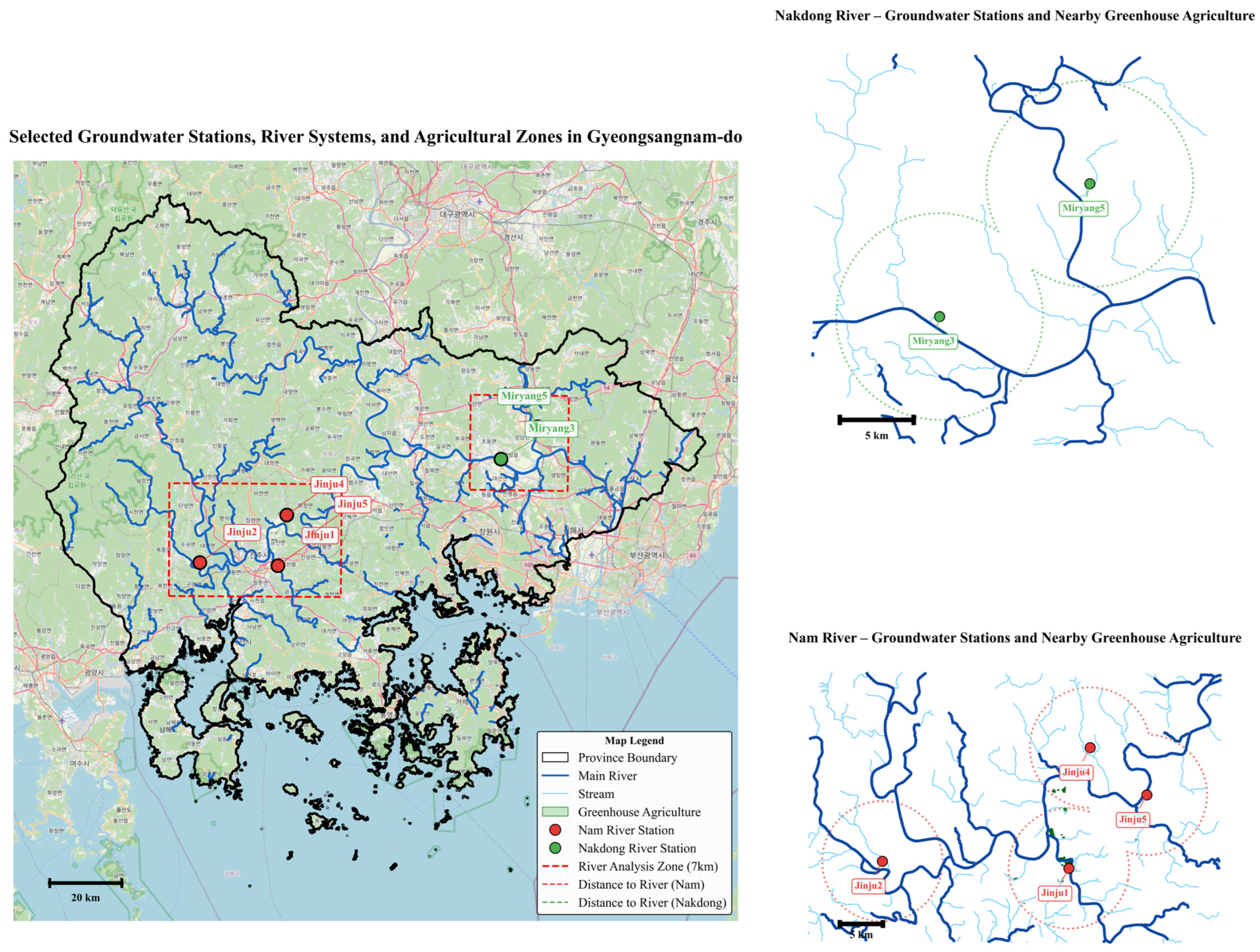
This study focuses on the cities of Miryang and Jinju in Gyeongsangnam-do Province, South Korea, which are widely recognized for their intensive greenhouse-based agricultural systems (Figure 1). During the winter season, GW pumping has been used for years (this study focused on pumping years from 2007–2025 based on station installation) as an economical heat source for water curtain cultivation. The dataset was obtained from stations within the Rural Groundwater Monitoring Network (RGMN), as mentioned in

Table 1. Descriptive statistics of selected GW monitoring stations near the Nam and Nakdong rivers in the Gyeongsangnam-do region.

River	Station	Distance from River (km)	Lat	Long	Depth (m)	Mean	Variable	Installation Year	Std.	CV (%)	Skewness	Min	Max
Nam River	Jinju1	0.19	35.1587	128.1533	159	21.75	GW Sea Level (m)	2007	1.34	6.14	−0.49	17.83	24.77
						538.63	EC (µS/cm)		91.06	16.91	0.27	318.58	769.60
						15.41	Temperature (°C)		0.23	1.46	−0.46	14.87	16.04
	Jinju2	0.77	35.1648	127.9587	60	38.11	GW Sea Level (m)	2016	8.95	23.49	−1.03	19.47	46.09
						420.02	EC (µS/cm)		45.11	10.74	−0.37	284.83	496.58
						14.92	Temperature (°C)		0.24	1.64	−0.24	14.26	15.60
	Jinju4	2.08	35.2617	128.1756	60	11.99	GW Sea Level (m)	2016	1.48	12.32	0.20	7.66	16.00
						718.52	EC (µS/cm)		48.94	6.81	−0.13	601.63	815.48
						16.71	Temperature (°C)		0.27	1.63	−0.24	16.09	17.20
	Jinju5	0.21	35.2214	128.2347	120	11.18	GW Sea Level (m)	2017	1.92	17.16	−1.65	3.66	15.44
						555.17	EC (µS/cm)		59.41	10.70	−0.75	367.04	644.58
						16.40	Temperature (°C)		0.01	0.08	−2.88	16.33	16.44
Nakdong River	Miryang3	0.61	35.3751	128.7097	66	−3.34	GW Sea Level (m)	2013	2.07	−61.97	0.13	−8.10	2.94
						659.86	EC (µS/cm)		7.74	1.17	−0.25	638.38	677.38
						16.47	Temperature (°C)		0.08	0.48	0.47	16.26	16.65
	Miryang5	0.98	35.4410	128.8011	60	−3.05	GW Sea Level (m)	2016	2.07	−67.98	−0.99	−8.38	−0.23
						333.67	EC (µS/cm)		4.33	1.30	0.01	325.13	347.33
						15.16	Temperature (°C)		0.05	0.33	−0.30	15.10	15.21

, and selected based on their proximity to greenhouse-dense areas and the availability and completeness of monitoring data.

Table 1 presents GW levels, physicochemical parameters, and statistical variability at monitoring stations on the Nam and Nakdong rivers in Gyeongsangnam-do. Depth (m) refers to the vertical distance from the ground surface to the monitoring well or sensor and is a measure of well construction. Groundwater sea level (m) is the hydraulic head (water level), defined as the level of GW relative to mean sea level, and describes the state of GW elevation and flow.

GW sea levels vary significantly across stations along the Nam River. Jinju1 (159 m) is the deepest well, with a stable GW of 21.75 m and low temporal variation (CV = 6.14%). Jinju2, on the contrary, has the highest mean GW level (38.11 m) and variability (CV = 23.49%), indicating that it is sensitive to seasonal recharge and pumping. Mean levels in Jinju4 and Jinju5 are lower (11.99 m and 11.18 m), with Jinju5 exhibiting pronounced negative skewness (−1.65), both of which are typical of episodic extremes associated with intensive agricultural abstraction. The electrical conductivity in the Nam River ranges from 420.02 to 718.52 µS/cm, with moderate variability (CV < 17%), suggesting stable conditions, though possibly influenced by minerals or artificial sources. GW is very buffered (14.9–16.7 °C; CV < 2%). On the other hand, Nakdong River stations (Miryang3 and Miryang5) have negative mean GW levels (−3.34 m and −3.05 m), indicating that they are hydraulically connected with the river, EC values are lower (minimum mean 333.67 µS/cm), and physicochemical variability is very low (CV ≤ 1.3%).

Hourly time-series datasets (2007–2025 based on station installation) from RGMN GW-level monitoring wells in the greenhouse-comprising agricultural regions of Gyeongsangnam-do, South Korea, were collected for different time periods, as shown in Table 1.

To minimize high-frequency noise without losing seasonal and interannual variations, the cleaned hourly data were converted to monthly GW means. The most common method of hydro-environmental trend analysis is monthly aggregation to balance signal retention and temporal smoothing [37]. Each monitoring station was then divided to produce a monthly time series, which was further divided into 12 independent sub-series, each based on a calendar month (January through December). This month-wise stratification enables the detection of intra-annual variability and seasonally differentiated long-term trends.

2.2. Methodology

2.2.1. Modified MK’s and Sen’s Slope Methods

Monotonic trends of every monthly GW-level sub-series were assessed by the non-parametric MK test [38,39]. The MK test is also distribution-free and resistant to outliers, and is appropriate for hydrological time series that often fail the normality and homoscedasticity conditions [40]. For a time series ($x_1,x_2,\dots ,x_n$), the MK test statistic $S$ is defined as:

$$S={\sum }_{k=1}^{n-1}.{\sum }_{j=k+1}^n\mathrm{s}\mathrm{g}\mathrm{n}(x_j-x_k),$$

(1)

where $x_j$ and $x_k$ are sequential observations, $n$ is the sample size, and the sign function $\mathrm{s}\mathrm{g}\mathrm{n}(\cdot )$ returns +1, 0, or −1 for positive, zero, or negative differences, respectively. A positive value of $S$ indicates an increasing trend, whereas a negative value indicates a decreasing trend. For series with $n\ge 10$, the variance of $S$ is computed while accounting for tied values as

$$\mathrm{V}\mathrm{A}\mathrm{R}(S)={\displaystyle \frac{1}{18}}[n(n-1)(2n+5)-{\sum }_{p=1}^g{t}_p(t_p-1)(2t_p+5)],$$

(2)

where $g$ is the number of tied groups and $t_p$ is the number of observations in the $p$^th group [40]. The standardized MK test statistic $Z_{MK}$ is then calculated as

$$Z_{MK}=\begin{array}{ccc}& {\displaystyle \frac{S-1}{\sqrt{\mathrm{V}\mathrm{A}\mathrm{R}\left(S\right)}}},& S>0,\\ \{& 0,& S=0,\\ & {\displaystyle \frac{S+1}{\sqrt{\mathrm{V}\mathrm{A}\mathrm{R}\left(S\right)}}},& S<0.\end{array}$$

$Z_{MK}$ under the null hypothesis of no monotonic trend, the distribution follows a standard normal distribution. The trends were believed to be statistically significant at 5% level when $\mid Z_{MK}\mid >1.96$ [41].

Since GW-level time series may be highly correlated, which can inflate the Type-I error rate of the classical MK test, the Hamed-Rao test with variance correction was used as the primary tool for trend detection [42]. This alteration modifies the variance of S to accommodate autocorrelation. Where this modified test was not possible to compute (e.g., because of inadequate record length), the original MK test was used as a backup.

The strength of observed trends was measured using Sen’s non-parametric slope estimator [43]. The slope between all pairs of observations was calculated for a given monthly sub-series.

$$d_k={\displaystyle \frac{x_j-x_i}{t_j-t_i}},i<j,$$

(3)

where $x_i$ and $x_j$ are GW-level observations at times $t_i$ and $t_j$, respectively. The Sen’s slope estimator $\beta$ is defined as the median of all $d_k$ values: $x_i$ and $x_j$ are GW-level observations at times $t_i$ and $t_j$, respectively. Sen’s slope estimator $\beta$ is the median of all $d_k$ values:

$$\beta =\mathrm{m}\mathrm{e}\mathrm{d}\mathrm{i}\mathrm{a}\mathrm{n}\left(d_k\right).$$

(4)

Sen’s slope is robust to outliers and does not assume linearity or normality, making it suitable for hydrological trend analysis. To facilitate interpretation, slope estimates were converted to meters per year (m year⁻¹) (${\beta }_{\mathrm{yr}}=\beta \times 12$). Based on both the sign and magnitude of ${\beta }_{\mathrm{yr}}$ trends were classified into qualitative categories such as minor depletion, strong recharge, or severe depletion using predefined threshold values (

Table 2. Trend classification scheme based on Sen’s slope magnitude and statistical significance.

Slope (m Year−1)	Direction	Classification
${\beta }_{\mathrm{yr}}\ge +0.10$	Increasing (↑)	Rapid recharge
$+0.05\le {\beta }_{\mathrm{yr}}<+0.10$	Increasing (↑)	Strong recharge
$+0.01\le {\beta }_{\mathrm{yr}}<+0.05$	Increasing (↑)	Moderate recharge
$0<{\beta }_{\mathrm{yr}}<+0.01$	Increasing (↑)	Minor recharge
${\beta }_{\mathrm{yr}}=0$ or $p\ge 0.05$	Stable (—)	No significant trend
$-0.01<{\beta }_{\mathrm{yr}}<0$	Decreasing (↓)	Minor depletion
$-0.05<{\beta }_{\mathrm{yr}}\le -0.01$	Decreasing (↓)	Moderate depletion
$-0.10<{\beta }_{\mathrm{yr}}\le -0.05$	Decreasing (↓)	Strong depletion
${\beta }_{\mathrm{yr}}\le -0.10$	Decreasing (↓)	Severe depletion

).

The hydrological year was split into two seasons to capture the prevailing hydrological and agricultural regimes of the study area, in accordance with local climate and GW-use activities. The winter (dry) season lasts from November to March and coincides with the phase of intensive GW abstraction during water-curtain greenhouse heating, a common practice in South Korean agriculture. The summer (wet) season runs from April to October and is characterized by higher precipitation, greater recharge capacity, and lower GW demand for heating [44]. This seasonal partitioning allows the behavior at the GW level to be directly compared in contrasting stress and recharge conditions.

2.2.2. DL-Based Methods

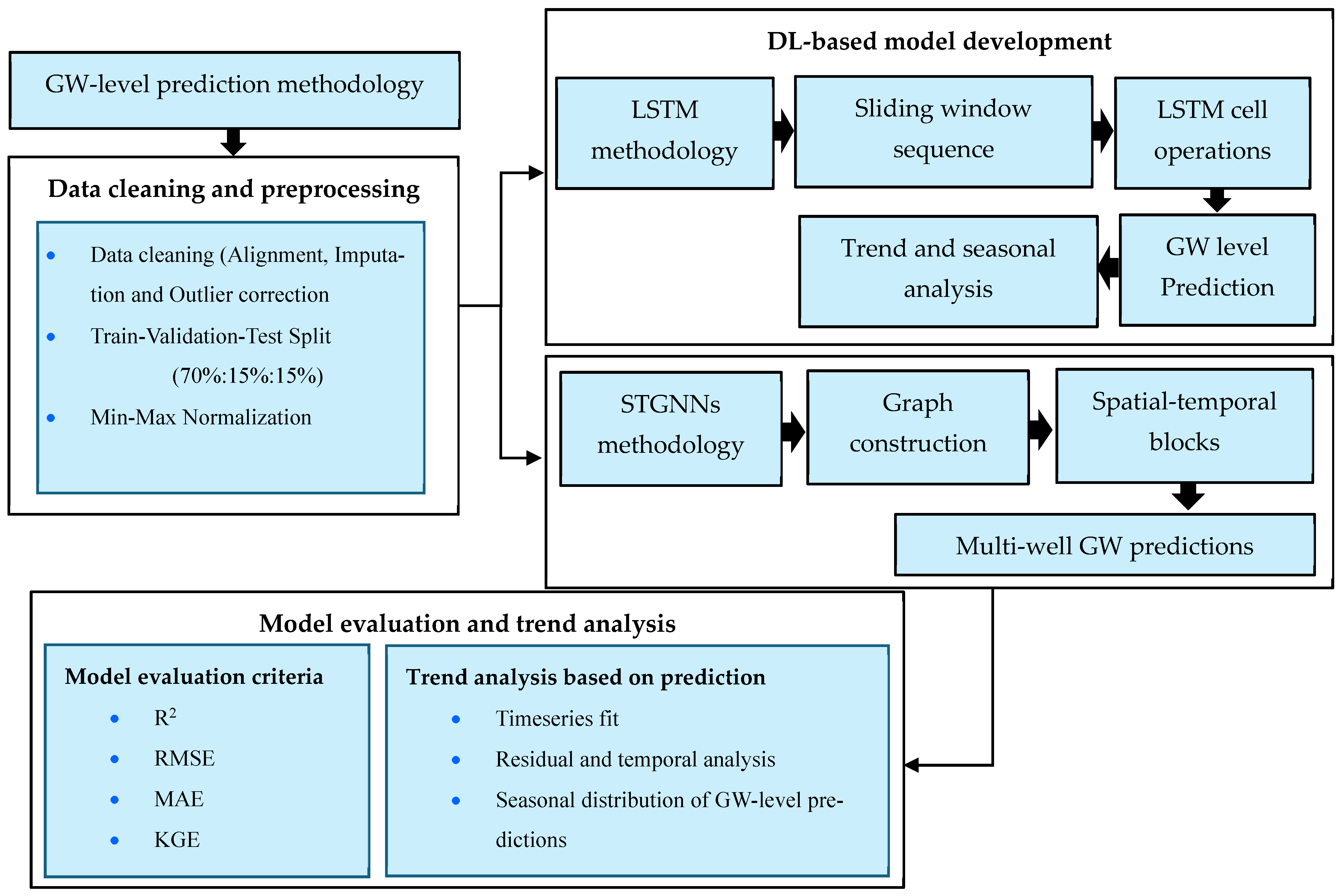
The study is an advancement in GW-level prediction, as it systematically trains and compares two advanced DL models, LSTM and STGNNs, as shown in Figure 2. The LSTM framework is trained to identify intricate temporal relationships, such as long-term persistence and seasonality, in individual monitoring wells using univariate time-series modeling. STGNN architecture leverages temporal dynamics and the spatial interdependence between wells by treating the aquifer system as a graph. By comparison, the STGNN explicitly models the evolution of time as well as the spatial interconnection between wells, enabling the modeling of aquifer connectivity at the scale and the synchronized pumping effect.

a. 

Data cleaning and train–validation–test splitting

Data cleaning of hourly GW records from RGMN stations (2007–2025) was performed before analysis. Synchronization of timestamps between wells and elimination of repeated or conflicting records to achieve a continuous hourly record were initially carried out to attain temporal alignment. The gaps (missing values) caused by sensor failure or by gaps in transmission have been filled by linear interpolation when the gap is less than 24 h long and by mean values of the month when the gap is longer than 24 h to ensure that seasonal effects are not distorted and artificial trends are not created.

The interquartile range (IQR) method was used to identify outliers due to sensor drift or sudden measurement errors, and flagged values were interpolated locally using nearby timestamps [45]. The hourly cleaning data were consequently summarized into monthly means for later use in DL-based analyses.

The only predictive variable for LSTM and STGNN models was monthly GW level (GW sea level, m), as GW level was directly proportional to the combined impacts of recharge, abstraction, and hydraulic connectivity. Physicochemical parameters (EC and temperature) were not considered as model inputs but were included solely for descriptive and interpretative analysis.

The monthly GW-level records at the station, available from the year of installation (2007–2017, depending on the station) through December 2025, were used as the available data for each monitoring well. The overall record length ranged from 96 to 216 months across wells, indicating differences in installation dates (Table 1).

To provide strong generalization evaluation and prevent information leakage, the time series of each well was separated into training, validation, and test data sets in chronological order:

$${\mathrm{y}}_i^{\mathrm{train}}=\left[y_{i,1},\dots ,y_{i,T_{\mathrm{train}}}\right],$$

$${\mathrm{y}}_i^{\mathrm{val}}=\left[y_{i,T_{\mathrm{train}}+1},\dots ,y_{i,T_{\mathrm{train}}+T_{\mathrm{val}}}\right],$$

$${\mathrm{y}}_i^{\mathrm{test}}=[y_{i,T_{\mathrm{train}}+T_{\mathrm{val}}+1},\dots ,y_{i,T}].$$

In this modeling, 70% of the data were used for training, 15% for validation, and 15% for testing, maintaining temporal position to simulate real-world forecasting conditions. To make the model’s training stable and faster, the Min-Max normalization of each of the wells separately was performed based on the statistics acquired only on the training subset:

$${\tilde{y}}_{i,t}={\displaystyle \frac{y_{i,t}-\mathrm{m}\mathrm{i}\mathrm{n}\left({\mathrm{y}}_i^{\mathrm{train}}\right)}{\mathrm{m}\mathrm{a}\mathrm{x}\left({\mathrm{y}}_i^{\mathrm{train}}\right)-\mathrm{m}\mathrm{i}\mathrm{n}\left({\mathrm{y}}_i^{\mathrm{train}}\right)}}.$$

(5)

The resulting normalized values are in the range [0, 1], and the same transformation parameters were used on the validation and test sets to avoid data leakage.

b. 

Long Short-term Memory

LSTM networks, a particular type of recurrent neural network (RNN), were described as capable of learning long-range temporal dependencies and overcoming the vanishing gradient problem inherent to traditional RNNs [46].

The univariate forecasting task was cast as a supervised learning problem using a sliding-window approach. For a predefined sequence length $L$ (e.g., 30 days), input–output pairs for well $w_i$ were constructed as

$${\mathrm{X}}_i^{\left(k\right)}=[{\tilde{y}}_{i,k},{\tilde{y}}_{i,k+1},\dots ,{\tilde{y}}_{i,k+L-1}],Y_i^{\left(k\right)}={\tilde{y}}_{i,k+L},$$

(6)

where $k=1,\dots ,T-L$.

Therefore, the input layer consisted of 12 successive monthly GW levels, and the output layer consisted of a prediction of the GW level for the next month.

This formulation trains the model to predict the next-month GW level conditioned on the preceding $L$ observations.

At each time step $t$, the LSTM cell updates its internal memory state through gated mechanisms defined as follows:

• Forget gate:

$$f_t=\sigma \left(W_f\left[h_{t-1},x_t\right]+b_f\right).$$

(7)

• Input gate and candidate state:

$$i_t=\sigma \left(W_i\left[h_{t-1},x_t\right]+b_i\right),{\tilde{c}}_t=\tanh \left(W_c\left[h_{t-1},x_t\right]+b_c\right).$$

(8)

• Cell state update:

$$c_t=f_t\odot c_{t-1}+i_t\odot {\tilde{c}}_t.$$

(9)

• Output gate and hidden state:

$$o_t=\sigma \left(W_o\right[h_{t-1},x_t]+b_o),h_t=o_t\odot \mathrm{t}\mathrm{a}\mathrm{n}\mathrm{h}\left(c_t\right).$$

(10)

where $\sigma (\cdot )$ denotes the sigmoid activation function and $\odot$ represents element-wise multiplication.

The adopted LSTM architecture uses a two-layer bidirectional LSTM (BiLSTM) with 128 hidden units, allowing the network to acquire not only forward but also backward temporal representations in the input sequence. The last hidden representation is fed into a fully connected layer with dropout (dropout rate = 0.2). Training is minimized using the mean squared error (MSE) loss with Adam and an initial learning rate of 0.001. Reducing the learning rate at a plateau and early stopping based on validation loss were used to improve convergence stability and reduce overfitting. Post-training, denormalized LSTM predictions ${\widehat{y}}_i\left(t\right)$ were analyzed to extract hydrologically meaningful components:

• Long-term trend:

Estimated via linear regression

$$\widehat{y}\left(t\right)=mt+b,$$

(11)

where the slope $m$ (m year⁻¹) quantifies long-term GW change.

• Seasonality:

Characterized using a sinusoidal model

$$S\left(t\right)=A\ast \mathrm{s}\mathrm{i}\mathrm{n}({\displaystyle \frac{2\pi t}{365.25}}+\varphi )+C,$$

(12)

yielding annual amplitude $A$ and phase shift $\varphi$.

• Monthly trends:

Linear regressions were fitted for each month to identify periods dominated by recharge or depletion processes.

c. 

Spatio-Temporal Graph Neural Network

An STGNN framework was developed to explicitly model aquifer-scale connectivity, treating GW monitoring wells as graph nodes and interactions between them as edges. It combines graph-based spatial learning with temporal sequence modeling [33].

• The aquifer system is represented as a weighted graph:

$$G=(V,E,A),$$

(13)

$V$ denotes the collection of wells, $E$ denotes the collection of edges, and $A\in {\mathbb{R}}^{N\times N}$ the adjacency matrix.

• Graph construction and adjacency matrix:

To achieve methodological reproducibility, the adjacency matrix was constructed using the Pearson correlation coefficient as the similarity measure for monthly GW-level time series. The similarity distance between the two wells i and j was determined as:

$$d\left(y_i,y_j\right)=1-{\rho }_{ij}$$

(14)

where ${\rho }_{ij}$ is the Pearson correlation coefficient between the normalized GW-level series of wells $i$ and $j$. Without the detailed data on the hydrogeological connectivity, the data-driven adjacency matrix was created with the help of GW time-series similarity:

$$A_{ij}=\exp \left(-{\displaystyle \frac{d(y_i,y_j{)}^2}{{\sigma }^2}}\right),$$

(15)

where $\sigma$ was changed to the standard deviation of all pairwise distances to regulate the rate at which edge weights decay.

A sparse graph structure of similarities (e.g., dynamic time warping or correlation distance) was obtained by removing edges whose $A_{ij}<0.3$ to obtain a sparse but hydraulically meaningful graph structure $d\left(\cdot \right)$ represents a distance metric based on similarities (e.g., dynamic time warping or correlation distance). The weak links were removed using thresholding to promote sparsity.

Each ST block consists of:

• Graph convolution (spatial learning):

$$H^{(l+1)}=\sigma \left({\tilde{D}}^{-1/2}\tilde{A}{\tilde{D}}^{-1/2}{H}^{\left(l\right)}{W}^{\left(l\right)}\right),$$

(16)

where $\tilde{A}=A+I_N$ includes self-loops and $\tilde{D}$ is the corresponding degree matrix.

• Gated temporal convolution (temporal learning):

$$H_{\mathrm{out}}=\mathrm{t}\mathrm{a}\mathrm{n}\mathrm{h}({\mathsf{\Theta }}_1\ast H_{\mathrm{spatial}})\odot \sigma ({\mathsf{\Theta }}_2\ast H_{\mathrm{spatial}}),$$

(17)

where $\ast$ denotes causal convolution. The STGNN processes tensor input.

$$X\in {\mathbb{R}}^{B\times L\times N},$$

(18)

where $B$ is the batch size, $L=12$ months is the length of the input sequence, and $N=6$ is the number of monitoring wells. Output is the forecasted GW level of all the wells in the following monthly time step.

To compare with the LSTM, the STGNN was trained on a composite loss function combining MSE and MAE, with Adam optimization, using the same training-validation-testing split. R², RMSE, and MAE were used to evaluate the model’s performance on the independent test set, as indicated in the Supplementary Material.

3. Results

This section presents detailed analysis outcomes in three sections: (1) historical seasonal GW-level trends based on non-parametric modified MK and Sen’s slope methods, and (2) DL-based prediction and temporal analysis of GW-level across all selected GW stations.

3.1. GW-Level Trend Analysis Based on the MK and Sen’s Slope Methods

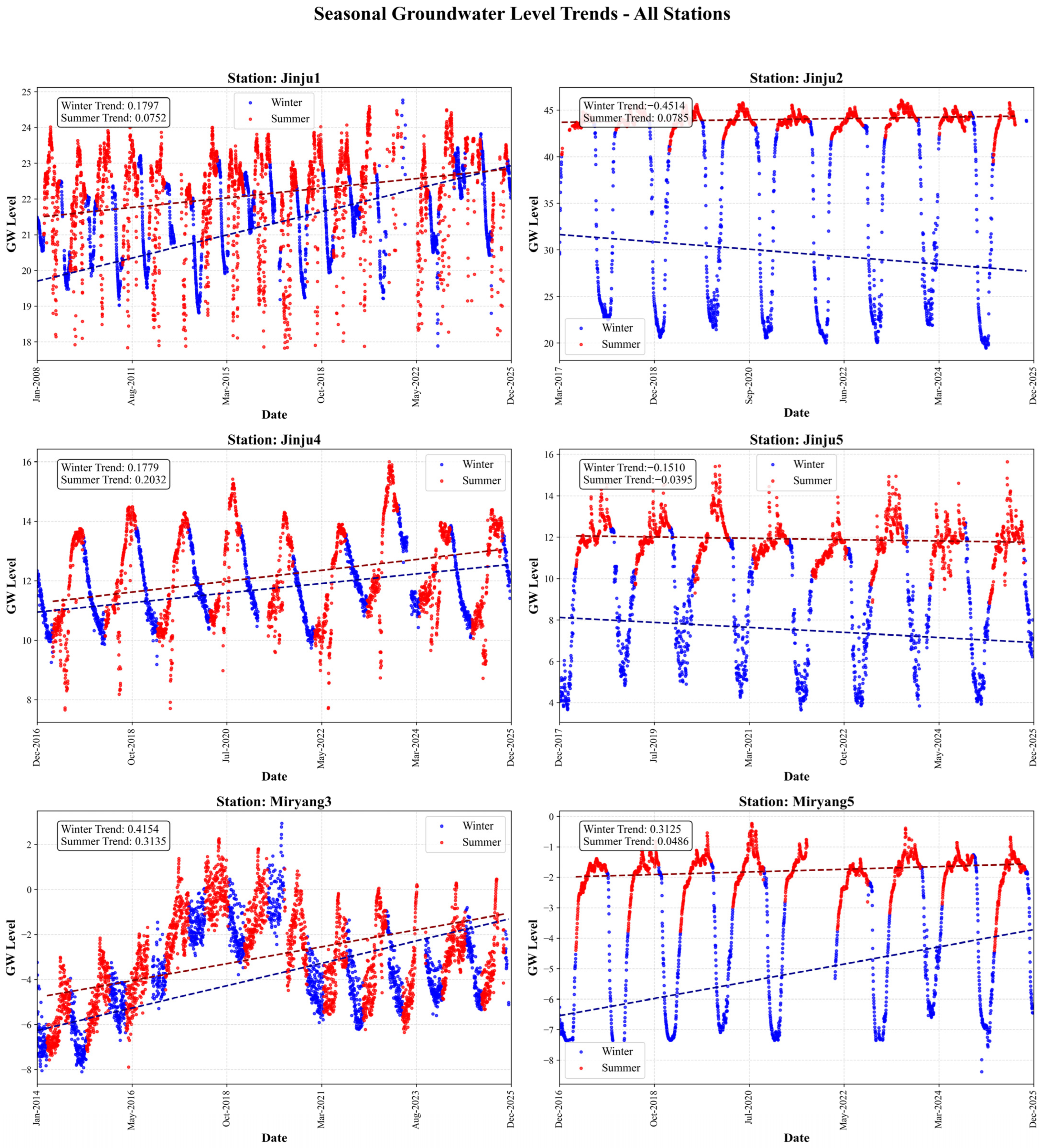
In this section, seasonal GW-level trends are presented using the modified MK and Sen slope estimators, clearly attributing observed GW variability to intensive greenhouse agriculture and related abstraction pressures. To capture the high seasonal asymmetry under the effect of water-curtain greenhouse heating, which is the primary agricultural activity in Gyeongsangnam-do, the analysis is separated into wet (summer) and dry (winter) seasons, as summarized in

Table 3. Seasonal trend analysis summary during wet and dry seasons over selected stations in Gyeongsangnam-do greenhouse agriculture systems.

Station	Data Duration	Summer (Wet Season)
		Slope_ Year	Slope_ Daily	p Value	Trend	Significance		Data Points	Mean GWL
Jinju1	2008–2025	0.0752	0.0002	0.0004	Increasing (↑)	TRUE	***	2923	22.1307
Jinju2	2017–2025	0.0785	0.0002	0.0367	Increasing (↑)	TRUE	*	1709	44.0113
Jinju4	2016–2025	0.2032	0.0006	0.005	Increasing (↑)	TRUE	**	1833	12.1921
Jinju5	2017–2025	−0.0395	−0.0001	0.4673	Stable (—)	FALSE	ns	1690	11.9083
Miryang3	2014–2025	0.3135	0.0009	0.2875	Stable (—)	FALSE	ns	2353	−2.9831
Miryang5	2016–2025	0.0486	0.0001	0.0549	Stable (—)	FALSE	ns	1841	−1.7786
Winter (Dry Season)
Jinju1	2008–2025	0.1797	0.0005	0	Increasing (↑)	TRUE	***	2304	21.2744
Jinju2	2017–2025	−0.4514	−0.0012	0.1223	Stable (—)	FALSE	ns	1199	29.6973
Jinju4	2016–2025	0.1779	0.0005	0.0115	Increasing (↑)	TRUE	*	1314	11.7171
Jinju5	2017–2025	−0.151	−0.0004	0.4899	Stable (—)	FALSE	ns	1172	7.5396
Miryang3	2014–2025	0.4154	0.0011	0.3185	Stable (—)	FALSE	ns	1651	−3.8376
Miryang5	2016–2025	0.3125	0.0009	0.0005	Increasing (↑)	TRUE	***	1093	−5.1943

Note: ***, **, and * denote statistical significance of monotonic trends at the 0.1%, 1%, and 5% levels, respectively, based on the MK test. ns indicates a non-significant trend (p ≥ 0.05).

and Figure 3.

The trend analysis was conducted using the original data, without imputation or data-filling methods, to maintain the reliability of the outcomes. In Table 3, the data points show the total number of daily GW-level observations used in the seasonal trend analysis for each station and season. The varying start years of monitoring and data availability across different stations result in varying numbers of observations, due to uneven record lengths and some missing measurements during the study period.

Statistically significant positive increasing trends are found in both seasons in Jinju1, which has the longest and most dense record (2008–2025; Table 3, Table S2 and Figure 3). The slope of the Sen is +0.0752 m year⁻¹ in summer and +0.1797 m year⁻¹ in winter, significant at p < 0.001. The winter trend is substantial because winter is the time of maximum GW abstraction for greenhouse heating. This opposite recovery indicates the synergistic effects of controlled pumping, the resilience of aquifer storage, and delayed recharge of adjacent hydrogeological units. Also, Table S1 shows high autocorrelation values (exceeding 0.92), which also support the use of the modified MK test and confirm the strength of the trends identified.

In comparison, Jinju2 shows a big seasonal difference in GW behavior. A statistically significant positive trend of +0.0785 m year⁻¹ (p = 0.0367) is observed during the wet season, indicating moderate recharge rates in line with increased precipitation and decreased pumping. The trend of the dry season, however, is negative (−0.4514 m year⁻¹) and not statistically significant (p = 0.1223), despite its large magnitude. This trend shows that there are occasional, but severe, abstraction events associated with greenhouse operations, leading to considerable interannual variability that, by itself, reduces statistical significance, regardless of the significant drawdown. The trend in the seasonal difference between winter and summer of +0.5299 m year⁻¹ (Table S1) is a quantitative measure of the overwhelming influence of anthropogenic stress in winter, and the insignificance of the difference is evidence of high interannual variability and a shorter record length.

Jinju4 is the most hydrologically stable station among the analyzed stations. The slopes of the trend of both summer and winter are positive and statistically significant: +0.2032 m year⁻¹ (p = 0.005) and +0.1779 m year⁻¹ (p = 0.0115), respectively. The low contrast between seasonal changes indicates that recharge processes are highly effective at offsetting the greenhouse-induced abstraction, likely due to favorable aquifer characteristics, reduced pumping density, or controlled abstraction activities. These slopes belong to the strong recharge category and exhibit a slight seasonal variation (+0.0253 m year⁻¹; Table S1), indicating that seasonal pumping does not significantly affect long-term GW recovery.

Jinju5 demonstrates the shortcomings of trend detection in highly variable, limited data from the dry season. The summer slope is small (−0.0395 m year⁻¹) and not significant (p = 0.4673), whereas the slope of winter Sen is −0.1510 m year⁻¹ but not significant (p = 0.4899) using just 1172 winter data points. It underscores the importance of slope magnitude, in conjunction with the variance structure and record length, in interpreting GW trends in intensively pumped agricultural systems.

The slopes of summer and winter at Miryang3 are positive (+0.3135 and +0.4154 m year⁻¹, respectively); however, neither trend is statistically significant (p > 0.2875). Although the apparent recharge rates are high, in the long run the average GW level is negative (−3.34 m), indicating continued hydraulic control rather than directional recovery. The near-equilibrium summer and winter slopes and insignificant seasonal disparity (−0.1019 m year⁻¹) imply that the recharge and abstraction dynamics are in balance with each other and thus high variability with no meaningful long-term trend. The fact that both the summer and winter slopes are almost equal (0.4154 and 0.3135 m year^−1, respectively; Table S1)

Miryang5 also shows seasonal asymmetry: the variable’s increasing trend is statistically significant only in the dry season. The slope of the winter Sen of +0.3125 m year⁻¹ (p = 0.0005) is in opposition to the marginal and insignificant summer trend of +0.0486 m year⁻¹ (p = 0.0549). This trend indicates a recent change in GW management practices in winter, including more efficient pumping, the use of alternative heating, or localized artificial recharge, which enable partial recovery even in high abstraction seasons. Moreover, total monthly recharge and depletion are given in the Supplementary File.

The trend analysis indicates that the dynamics, both spatially and seasonally, are not uniform in greenhouse-dominated GW systems. The intensity, timing, and spatial coordination of GW-driven pumping of greenhouse gases are controlled primarily by site-specific geological features, including aquifer connectivity and proximity to rivers.

Findings from trend analysis, presented as summaries in Table 3, Tables S1 and S2, and Figure 3, support the conclusion that GW patterns in greenhouse agricultural systems in Gyeongsangnam-do are neither spatially homogeneous nor seasonally even. Summer trends are usually minor and less significant, whereas winter trends have greater magnitudes, greater variability, and, in many cases, more substantial statistical indications. The slopes of Sen vary quantitatively across seasons, with Sen values ranging from −0.0151 to 1.7002 m year⁻¹, and statistically significant trends are found only when the slope magnitude, record length, and variance structure are consistent. The use of the modified MK test is critical for addressing autocorrelation and making sound inferences.

3.2. DL Based on GW-Level Temporal Analysis

The relative comparison of the LSTM and STGNN models indicates that GW dynamics in greenhouse agricultural systems are highly non-linear, seasonally abrupt, and spatially linked.

Across the different stations, the STGNN outperforms the LSTM, with R² ranging from 0.799 to 0.994. This most substantial enhancement is at Jinju1 (R² growth of 47.95%), indicating that at this station, GW variability is strongly influenced by lateral flow and coordinated pumping between the surrounding greenhouse complexes, which a strictly time-based model cannot describe.

Stations Jinju2, Miryang3, and Miryang5 show lower R² increments (4–5%), indicating that local temporal persistence predominates GW behavior at those locations. Nevertheless, STGNN does not lose its leads, remaining as strong, or even stronger, in heterogeneous hydrogeological environments.

The STGNN has higher explanatory power across all six monitoring stations, with R² ranging from 0.799 to 0.994, higher than those of the LSTM, which range from 0.555 to 0.954 (

Table 4. Overall summary of DL-based models over all stations for GW level predictions.

Station		Jinju1	Jinju2	Jinju4	Jinju5	Miryang3	Miryang5
R2	STGNN	0.821	0.992	0.961	0.951	0.799	0.994
	LSTM	0.555	0.946	0.771	0.751	0.768	0.954
	Improvement (%)	47.951	4.778	24.632	26.669	4.049	4.247
RMSE	STGNN	0.511	0.926	0.29	0.378	0.614	0.162
	LSTM	0.783	2.324	0.689	0.825	0.61	0.458
	Improvement (%)	34.687	60.166	57.894	54.182	−0.529	64.58
MAE	STGNN	0.289	0.719	0.194	0.235	0.468	0.095
	LSTM	0.449	1.567	0.57	0.65	0.462	0.334
KGE	STGNN	0.852	0.925	0.965	0.962	0.801	0.961
	LSTM	0.783	0.956	0.714	0.633	0.785	0.851

). It has been especially improved at Jinju1, where R² increased by 47.95 (0.555 to 0.821). This high gain indicates that GW variations at Jinju1 are strongly influenced by non-local effects, including lateral GW movement and multiphase pumping in nearby greenhouse complexes, which a single-well temporal model cannot capture. Smaller but statistically significant gains are observed at Jinju4 and Jinju5, with R² of 24.63 and 26.67, respectively, further underscoring the importance of spatial interactions in seasonal GW behavior in these locations.

Stations Jinju2, Miryang3, and Miryang5 show smaller increases in R², ranging from 4.0 to 4.8%. These smaller returns suggest that temporal persistence already accounts for a major portion of the variation at these sites, likely because of stable pumping regimes or increased local recharge. However, the STGNN performs as well as, or even better than, in such situations, demonstrating its strength in heterogeneous hydrogeological environments. The high R² of 0.994 at Miryang5 for the STGNN indicates that the model reproduces the observed GW variability perfectly, supporting its potential to generalize the seasonal dynamics in space and time.

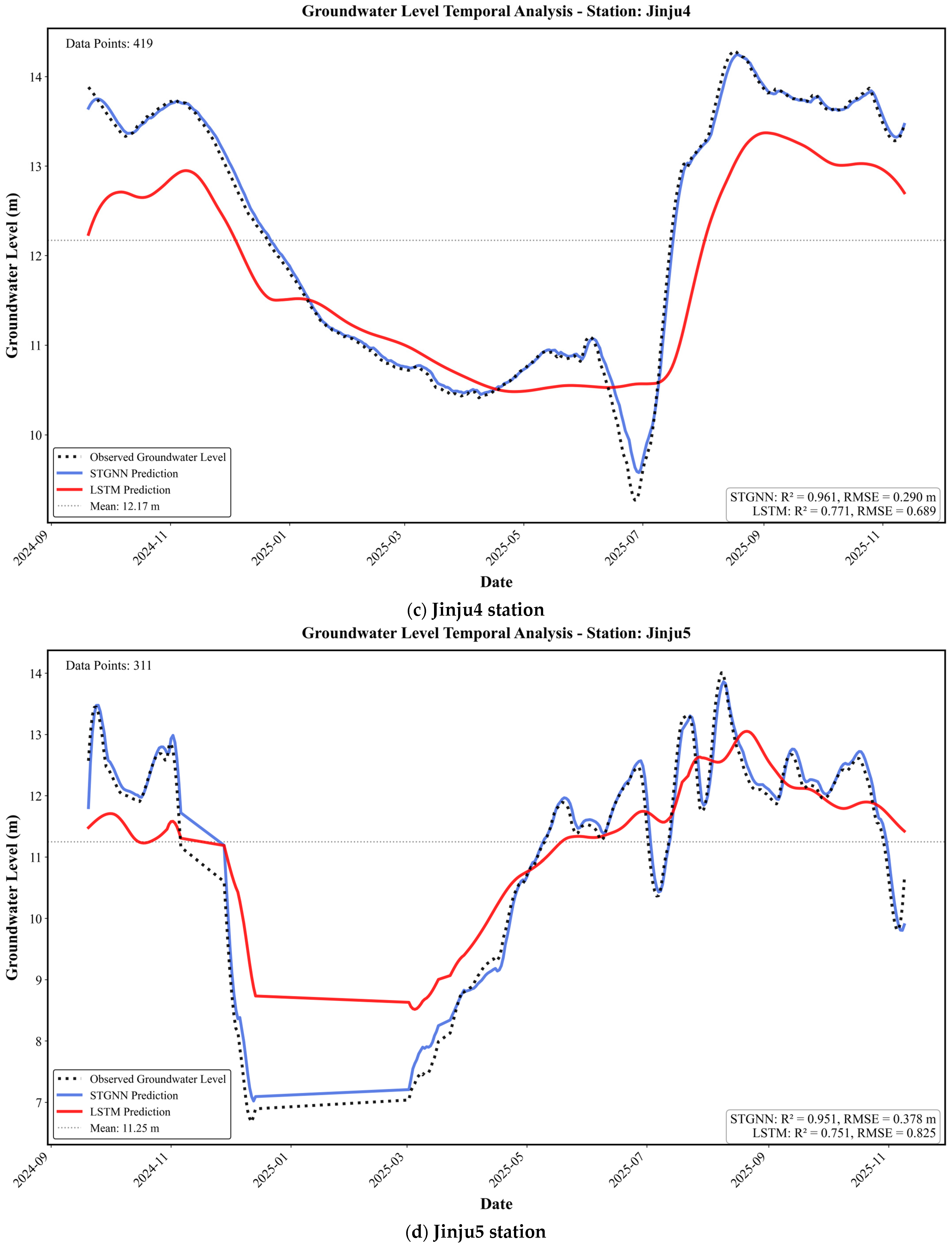
Measurements based on errors give extra information about model behavior. The STGNN has significant error reductions at most of the stations, with the most significant error reductions at Jinju2, Jinju4, Jinju5, and Miryang5 of 60.17, 57.89, 54.18, and 64.58, respectively (Table 4). Such significant decreases suggest that the STGNN not only enhances correlation but also significantly lowers absolute deviations between the predicted and observed GW levels. It is critical to adopt realistic GW management, as a smaller prediction error indicates higher evaluation quality of the magnitude of drawdown and the timing of recovery under intensive greenhouse water use. Miryang3 is the only one with a slight increase in RMSE, reaching 0.614 m (STGNN), with a slight decrease of −0.53%. This minor worsening does not compromise the overall excellence of the spatio-temporal approach, given the small scale of this difference and the simultaneous increase in R² and KGE.

These findings are supported by the MAE results, which show that STGNN’s absolute bias was significantly smaller at 5 of 6 stations. For example, MAE at Jinju2 reduces from 1.567 m under LSTM to 0.719 m under STGNN, whereas at Miryang5 it reduces from 0.334 m to 0.095 m. Such cuts suggest that not only are the predictions of STGNN more accurate statistically, but also that they are closer to the observed GW levels on a daily basis. At Miryang3, the MAE is almost identical across the two models (0.468 m in STGNN and 0.462 m in LSTM), which again indicates that there is no significant spatial dependence at this station and not that the models are inadequate.

The KGE also supports STGNN’s ability to generate hydrologically significant features from GW time series. KGE at Jinju4 and Jinju5 is significantly higher at 0.965 and 0.962, respectively, indicating that the STGNN is more balanced in terms of correlation, variability, and bias. Even though the LSTM has a slightly higher KGE at Jinju2 (0.956, compared to 0.925), the STGNN still performs better than the LSTM in RMSE and R 2 at this station, implying that the slight differences in the representation of variance do not supersede the total predictive gains.

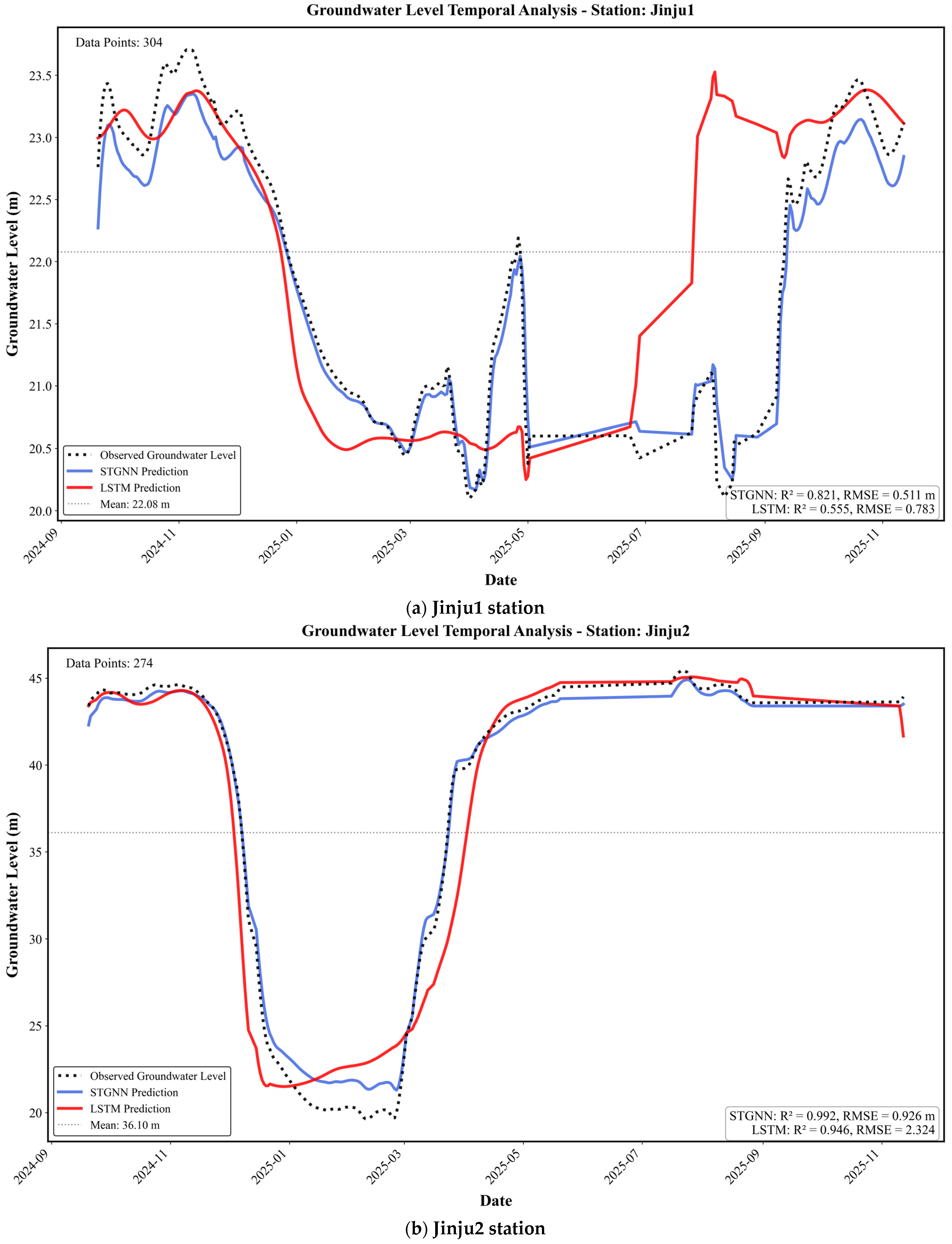
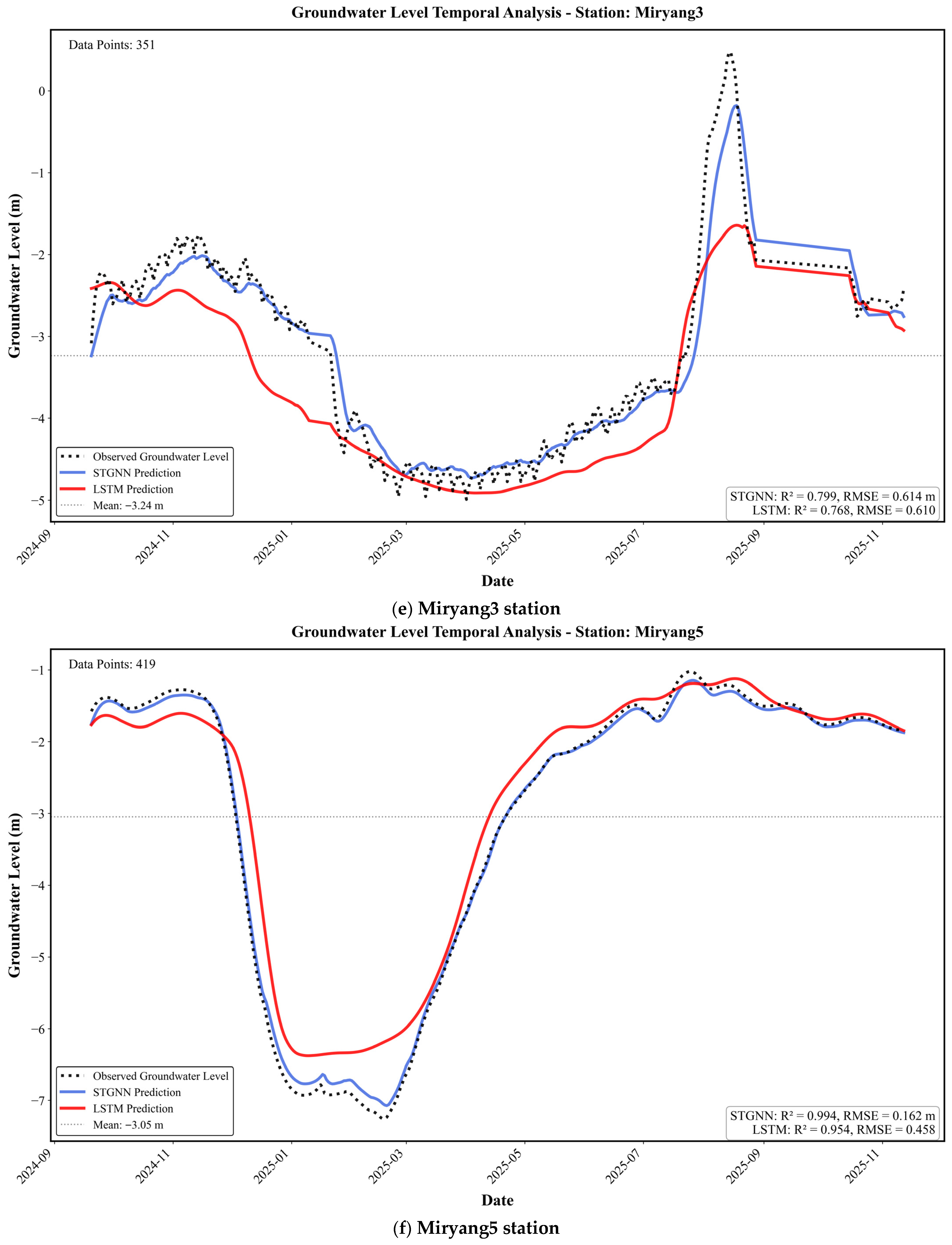
Figure 4 from the temporal analysis is an important qualitative supplement to these quantitative findings and provides a direct rationale for conducting the study on GW seasonality. The GW series recorded at Miryang5 shows a substantial seasonal drawdown of about −8 m in winter, followed by a slow increase to summer, a pattern familiar to intensive winter GW-heated greenhouse heating. The STGNN is much more attentive to the extent and timing of this drawdown and its subsequent recovery than the LSTM, but the LSTM over-smooths the decline and recovery, as shown in the Miryang5 temporal analysis figure. This visual consensus aligns with the substantial decrease in RMSE from 0.458 m (LSTM) to 0.162 m (STGNN) and the increase in R² from 0.954 to 0.994.

The same behavior is observed at Jinju1, where the peaks and valleys of abrupt drops and recoveries associated with pumping events are better modeled by the STGNN than by the LSTM. The LSTM shows excessive smoothing and a slow response to sharp decreases, whereas the STGNN better follows observed variability, consistent with an R² improvement of almost 48% and a lower RMSE of 34.69. These findings indicate that temporal-only models are ineffective at capturing rapid transitions driven by spatially coordinated pumping, whereas STGNNs benefit from shared information across wells.

Jinju2 and Jinju4 show a noticeable seasonal cycle, with low-water periods lasting longer during winter and conditions becoming more stable afterwards. The STGNN accurately replicates the intensity and duration of such seasonal lows, whereas the LSTM predicts depletion and recovery and consequently systematically underestimates and overestimates, respectively. Such a move is consistent with the high changes in RMSE and MAE recorded in Table 4.

Miryang3 has notable outliers. Though the STGNN is gaining a slight increase in R², RMSE decreases insignificantly (by −0.53%), and MAE remains almost the same. This practice indicates the hegemony of local controls rather than model incompetence. Miryang3 is 0.61 km from the Nakdong River, and its continuously negative mean GW level indicates high hydraulic connectivity between the river and the aquifer. The effect of this river-based boundary condition is that the spatial pumping signals from wells in the immediate environs are likely to be obscured, making medium-range spatial learning less effective.

Also, the high-frequency variability at Miryang3 is due to localized pumping patterns associated with nearby greenhouse clusters and sudden changes in river stage, rather than sensor noise. The STGNN cannot effectively filter these signals using spatial aggregation, as they are site-specific and poorly correlated with neighboring stations. For example, at stations such as Jinju1 or Jinju5, pumping is spatially synchronized. This is why spatial coherence has less predictive value at Miryang3.

The findings show that the dynamics of GW in greenhouse agricultural sites in Gyeongsangnam-do exhibit strong seasonal patterns and spatial interactions among wells. The STGNN is highly effective, demonstrating that the explicit representation of these interactions is a meaningful step towards GW-level prediction and directly addresses the study’s aim. In addition, the DL models’ ability to isolate seasonal drawdowns, recovery patterns, and long-term trends in the predicted time series justifies the study’s focus on GW seasonal trends. The findings indicate the importance of spatio-temporal DL as a scientifically valid and applicable method of GW monitoring and management in highly cultivated greenhouse areas.

4. Discussion

In this study, the evaluation of seasonal GW dynamics and predictive model performance in greenhouse agricultural systems of Gyeongsangnam-do, South Korea, is presented through the application of non-parametric statistical trend analysis and high-tech DL methods. These findings show that GW behavior in such systems is highly seasonal, spatially heterogeneous, and strongly dependent on anthropogenic pumping associated with winter greenhouse cultivation. In addition to concluding the statistical trends, the analysis also provides insight into the physical and anthropogenic processes that have led to both rising and falling GW levels observed throughout the study area.

The trend analysis, based on the modified MK test and the Sen slope estimator, indicates significant seasonal differences in GW level behavior. The increasing and decreasing trends were statistically significant only in the winter (dry) season; in summer (wet season), trends were weaker and not significant. It is a seasonal asymmetry that can be explained by the prevalence of anthropogenic abstraction in winter, especially in water-curtain greenhouse cultivation, which has been well documented as a key cause of seasonal GW depletion in southern Korea [13,14,16]. The measured wintertime GW decreases at various stations are consistent with previous field-based and modeling research in the Miryang and Nakdong River alluvial plains, where high pumping rates occur between November and February, resulting in significant drawdown and changes in stream-aquifer interactions [13,15]. These declining trends are explained by the high rates of intensive pumping for greenhouse heating, low natural recharge during the dry season, and delayed aquifer recovery due to storage effects.

In contrast, those stations with increasing or decreasing trends are attributed to several hydrogeological and hydrological processes. Also, locations with lower greenhouse gas density or lower pumping intensity exhibit weaker declining signals, indicating that human pressure is not spatially uniform across the study region. Notably, the use of the modified MK test, which accounts for serial autocorrelation, was essential to ensuring strong trend detection. Storage effects and delayed recharge processes make the GW time series autocorrelated, and ignoring this property may lead to an overestimation of trend significance [37,42,47]. The observation that trends of only large magnitude, long record, and variance structure achieved statistical significance supports serious methodological attention to trend studies of GW, especially in managed agricultural systems.

The localized behavior of GW in relation to greenhouse agriculture is further revealed by the spatial heterogeneity in GW trends across monitoring stations. Aquifer properties, well depth, proximity to rivers, and pumping intensity may explain the significant declines observed in winter at some stations and the weak or no trends at others. Specifically, rapid recovery and periodic increases in stream stations within hydraulically connected alluvial plains near river channels are linked with stream-aquifer exchange. In contrast, the persistently decreasing trends at relatively isolated or deeper aquifer stations can be attributed to limited recharge pathways. The same spatially varying responses have been documented at the regional and national levels in Korea [5,31], with the key point being that GW management strategies should be based on local hydrogeological and land-use contexts rather than homogeneous regional assumptions.

The DL–based temporal prediction results provide additional insight into the complexity of GW dynamics in the study area. The evaluation results indicated that the STGNN performed better than the LSTM model at most stations and seasons, with lower prediction errors and greater ability to reproduce observed seasonal variations. Although LSTM models are highly adaptable for modeling long-term temporal variations in hydrological time series [24,46,48], these studies treat monitoring stations as independent sequences and thus do not explicitly model the interactions among wells. On the contrary, the STGNN architecture is designed to learn temporal dynamics alongside spatial connectivity, enabling it to capture lateral GW flow, standard pumping signals, and regional recharge patterns [33].

The overall better performance of STGNN in the current study is consistent with recent developments in data-driven GW modeling, which increasingly recognize the importance of spatio-temporal learning in human-influenced aquifer systems [18,30]. Spatial coupling is vital for determining GW dynamics in greenhouse-dominated landscapes, where pumping schedules are synchronized across adjacent farms, and aquifers are hydraulically linked. The fact that STGNN can exploit these dependencies is reflected in its superior predictive accuracy compared to purely temporal models, such as LSTMs.

The findings have implications of different significance for the management of water resources. First, the statistically significant seasonal GW reduction in most stations during winter suggests the susceptibility of greenhouse agricultural systems to excessive use during the dry season. Whilst GW is thought to be an essential source of climatic variability in monsoon-dominated areas [1], long-term pumping without sufficient recharge can reduce long-term storage, escalate the cost of pumping, and decrease local surface water ecosystems [2]. The identification of locations with increasing or steady trends suggests that natural recharge areas and stream-linked aquifers act as buffers and can be prioritized in managed aquifer recharge or protection to maintain the balance of regional GW. Second, the usefulness of DL models, particularly STGNN, implies that data-driven forecasting tools can support initiative-taking GW management, such as seasonal drawdowns and GW hotspot identification.

Statistical trend analysis and its DL-based prediction can be considered a methodological strength of the study. Trend analysis identifies long-term variations that can be explained, but DL models capture short-term variations and non-linear behavior. Such mixed approaches have received growing attention in recent reviews as a means of balancing interpretability and predictive power in GW studies [21,29]. In Gyeongsangnam-do, this combined system may be used to inform regulatory planning and operational decision-making, such as changing the pumping schedule or implementing controlled aquifer recharge during periods of high demand.

The STGNN 30-day GW level predictions can be directly incorporated into a seasonal management program for the winter pumping season (November–March). Since the model can also predict the timing and relative scale of drawdown across spatially related wells, forecasts can serve as early warning signals of impending critical depletion. Historical thresholds based on Sen slope classifications can be compared with predicted levels to inform management interventions such as staggered pumping, reduced abstraction, alternative heating use, or managed recharge.

Despite the advancement, the current study has some limitations. To start, the analysis was based on GW-level measurements, with no direct use of pumping rate, greenhouse density, or irrigation patterns. Although the patterns of seasonality are highly indicative of pumping-driven processes, the lack of direct data on abstraction makes it difficult to attribute the trends solely to agricultural activities. Second, the monitoring period was not uniform across all stations, which could have affected the ability to detect trends and the stability of model training at some sites. Third, there was no explicit modeling of climate variability and extreme events, including multi-year droughts, despite these factors being known to affect GW levels in Korea [6,9].

Future studies should consequently aim to combine GW level measurements with comprehensive pumping data, land-use data, and climate variables to address the need to separate natural and human-made controls on GW dynamics. More interpretable models could also be achieved by adding hybrid physics-informed and data-driven models without losing the predictive abilities of DL models [20]. Also, incorporating climate change scenarios into the spatio-temporal modeling framework would provide valuable insights into the long-term sustainability of greenhouse agriculture amid rising water stress.

5. Conclusions

This study presents a quantitative evaluation of GW seasonality in greenhouse agricultural systems in Gyeongsangnam-do by integrating non-parametric methods. The modified MK and Sen’s slope analyses show that GW behavior is strongly seasonal and spatially heterogeneous, with winter (dry-season) trends more pronounced and variable than summer trends. This asymmetry of the seasons is the result of the preponderance of intensive GW withdrawal in winter linked to water-curtain greenhouse heating. The increasing trends at some of the chosen stations (e.g., Jinju1 and Jinju4) are statistically significant, indicating localized recovery, whereas weak or non-significant trends at others reflect the combined effects of short data records, high interannual variability, and heterogeneous hydrogeological conditions.

The predictive modeling findings indicate that GW dynamics in greenhouse-dominated landscapes are highly non-linear and spatially coupled. The spatio-temporal GN neural network was significantly better than the LSTM model at most stations, with significant increases in R² (up to 48%) and significant decreases in RMSE and MAE, especially in winter. These advantages confirm that explicit modeling of spatial connectivity between wells is essential to represent synchronized pumping signals, lateral GW movement, and group recharge–depletion processes, which purely time-based models cannot capture. The STGNN’s ability to replicate sharp seasonal drawdowns and recoveries indicates its appropriateness for operational GW forecasting of highly managed agricultural aquifers.

The study’s findings suggest that the integrated statistical-DL model is more predictive and interpretable and is a strong tool for evaluating seasonal GW. The findings emphasize the vulnerability of greenhouse agricultural systems to overwinter extraction and support the use of spatiotemporal predictive models to inform sustainable pumping control, seasonal water management, and long-term GW protection as stress from climatic and anthropogenic pressures increases.

References

1. Scanlon, B.R.; Fakhreddine, S.; Rateb, A.; de Graaf, I.; Famiglietti, J.; Gleeson, T.; Grafton, R.Q.; Jobbagy, E.; Kebede, S.; Kolusu, S.R.; et al. Global water resources and the role of groundwater in a resilient water future. Nat. Rev. Earth Environ. 2023, 4, 87–101. [Google Scholar] [CrossRef] [Scilit]
2. Shaikh, M.; Birajdar, F. Groundwater and ecosystems: Understanding the critical interplay for sustainability and conservation. EPRA Int. J. Multidiscip. Res. 2024, 10, 181–186. [Google Scholar]
3. Wada, Y.; Van Beek, L.P.; Weiland, F.C.S.; Chao, B.F.; Wu, Y.H.; Bierkens, M.F. Past and future contribution of global groundwater depletion to sea-level rise. Geophys. Res. Lett. 2012, 39, 295. [Google Scholar] [CrossRef] [Scilit]
4. Famiglietti, J.S. The global groundwater crisis. Nat. Clim. Change 2014, 4, 945–948. [Google Scholar] [CrossRef] [Scilit]
5. Lee, B.; Hamm, S.-Y.; Jang, S.; Cheong, J.-Y.; Kim, G.-B. Relationship between groundwater and climate change in South Korea. Geosci. J. 2014, 18, 209–218. [Google Scholar] [CrossRef] [Scilit]
6. Karunakalage, A.; Lee, J.-Y.; Daqiq, M.T.; Cha, J.; Jang, J.; Kannaujiya, S. Characterization of groundwater drought and understanding of climatic impact on groundwater resources in Korea. J. Hydrol. 2024, 634, 131014. [Google Scholar] [CrossRef] [Scilit]
7. Scanlon, B.R.; Zhang, Z.; Save, H.; Sun, A.Y.; Schmied, H.M.; van Beek, L.P.H.; Wiese, D.N.; Wada, Y.; Long, D.; Reedy, R.C.; et al. Global models underestimate large decadal declining and rising water storage trends relative to GRACE satellite data. Proc. Natl. Acad. Sci. USA 2018, 115, E1080–E1089. [Google Scholar] [CrossRef] [Scilit]
8. Shah, T. Groundwater Governance and Irrigated Agriculture; No. 19; Global Water Partnership (GWP): Stockholm, Sweden, 2014. [Google Scholar]
9. Kang, M.; Hao, Y.; Choi, M. The effects of flash drought on the terrestrial ecosystem in Korea. J. Hydrol. 2023, 624, 129874. [Google Scholar] [CrossRef] [Scilit]
10. Seo, J.Y.; Lee, S.-I. Satellite data-driven deep learning approach for monitoring groundwater drought in South Korea. In Proceedings of the IGARSS 2022-2022 IEEE International Geoscience and Remote Sensing Symposium, Kuala Lumpur, Malaysia, 17–22 July 2022; IEEE: New York, NY, USA, 2022; pp. 6312–6315. [Google Scholar]
11. Konikow, L.F. Long-term groundwater depletion in the United States. Groundwater 2015, 53, 2–9. [Google Scholar] [CrossRef] [Scilit]
12. Döll, P.; Schmied, H.M.; Schuh, C.; Portmann, F.T.; Eicker, A. Global-scale assessment of groundwater depletion and related groundwater abstractions: Combining hydrological modeling with information from well observations and GRACE satellites. Water Resour. Res. 2014, 50, 5698–5720. [Google Scholar] [CrossRef] [Scilit]
13. Lee, H.; Koo, M.H.; Kim, Y. Impacts of seasonal pumping on stream-aquifer interactions in Miryang, Korea. Groundwater 2017, 55, 906–916. [Google Scholar] [CrossRef] [Scilit] [PubMed]
14. Lee, H.; Koo, M.H.; Oh, S. Modeling stream-aquifer interactions under seasonal groundwater pumping and managed aquifer recharge. Groundwater 2019, 57, 216–225. [Google Scholar] [CrossRef] [Scilit] [PubMed]
15. Kim, G.B. Application of analytical solution for stream depletion due to groundwater pumping in Gapcheon watershed, South Korea. Hydrol. Process. 2010, 24, 3535–3546. [Google Scholar] [CrossRef] [Scilit]
16. Ha, K.; Lee, E.; An, H.; Kim, S.; Park, C.; Kim, G.-B.; Ko, K.-S. Evaluation of seasonal groundwater quality changes associated with groundwater pumping and level fluctuations in an agricultural area, Korea. Water 2021, 13, 51. [Google Scholar] [CrossRef] [Scilit]
17. Wang, W.; Tian, H.; Yang, G.; Liu, B.; Pan, Y.; Ding, G.; Xu, X.; Dan, Y.; Cui, M.; Gao, Y. Dynamic variation of groundwater level and its influencing factors in typical oasis irrigated areas in Northwest China. Open Geosci. 2023, 15, 20220493. [Google Scholar] [CrossRef] [Scilit]
18. Jing, H.; Tian, H.; Yang, G.; Liu, B.; Pan, Y.; Ding, G.; Xu, X.; Dan, Y.; Cui, M.; Gao, Y. Comparison and interpretation of data-driven models for simulating site-specific human-impacted groundwater dynamics in the North China Plain. J. Hydrol. 2023, 616, 128751. [Google Scholar] [CrossRef] [Scilit]
19. Feng, G.; Jin, W.; Ouyang, Y.; Huang, Y. The role of changing land use and irrigation scheduling in groundwater depletion mitigation in a humid region. Agric. Water Manag. 2024, 291, 108606. [Google Scholar] [CrossRef] [Scilit]
20. Zhu, F.; Sun, Y.; Han, M.; Hou, T.; Zeng, Y.; Lin, M.; Wang, Y.; Zhong, P.-A. A robust bayesian multi-machine learning ensemble framework for probabilistic groundwater level forecasting. J. Hydrol. 2025, 650, 132567. [Google Scholar] [CrossRef] [Scilit]
21. Ali, A.S.A.; Jazaei, F.; Babakhani, P.; Ashiq, M.M.; Bakhshaee, A.; Waldron, B. An overview of deep learning applications in groundwater level modeling: Bridging the gap between academic research and industry applications. Appl. Comput. Intell. Soft Comput. 2024, 2024, 9480522. [Google Scholar] [CrossRef] [Scilit]
22. Ahn, S.-M.K.B.-I. Estimation of the Change in Ground Water Level using Regression Analysis. J. Korean Soc. Agric. Eng. 2011, 53, 51–58. [Google Scholar] [CrossRef] [Scilit]
23. Mohanasundaram, S.; Udmale, P.; Shrestha, S.; Baghel, T.; Doshi, S.C.; Narasimhan, B.; Kumar, G.S. A new trend function-based regression kriging for spatial modeling of groundwater hydraulic heads under the sparse distribution of measurement sites. Acta Geophys. 2020, 68, 751–772. [Google Scholar] [CrossRef] [Scilit]
24. Roshni, T.; Jha, M.K.; Drisya, J. Neural network modeling for groundwater-level forecasting in coastal aquifers. Neural Comput. Appl. 2020, 32, 12737–12754. [Google Scholar] [CrossRef] [Scilit]
25. Nan, T.; Cao, W.; Wang, Z.; Gao, Y.; Zhao, L.; Sun, X.; Na, J. Evaluation of shallow groundwater dynamics after water supplement in North China Plain based on attention-GRU model. J. Hydrol. 2023, 625, 130085. [Google Scholar] [CrossRef] [Scilit]
26. Roy, D.K.; Hashem, A.A.; Reba, M.L.; Leslie, D.L.; Nowlin, J. A maximal overlap discrete wavelet packet transform coupled with an LSTM deep learning model for improving multilevel groundwater level forecasts. Discov. Water 2024, 4, 16. [Google Scholar] [CrossRef] [Scilit]
27. Sun, J.; Hu, L.; Li, D.; Sun, K.; Yang, Z. Data-driven models for accurate groundwater level prediction and their practical significance in groundwater management. J. Hydrol. 2022, 608, 127630. [Google Scholar] [CrossRef] [Scilit]
28. Zhang, D.; Liu, X.; Simmons, C.T.; Zhang, L.; Zhang, Q. Changes in groundwater levels across China from 2005 to 2016. J. Hydrol. 2023, 623, 129781. [Google Scholar] [CrossRef] [Scilit]
29. Khan, J.; Lee, E.; Balobaid, A.S.; Kim, K. A comprehensive review of conventional, machine leaning, and deep learning models for groundwater level (GWL) forecasting. Appl. Sci. 2023, 13, 2743. [Google Scholar] [CrossRef] [Scilit]
30. Igwebuike, N.; Ajayi, M.; Okolie, C.; Kanyerere, T.; Halihan, T. Application of machine learning and deep learning for predicting groundwater levels in the West Coast Aquifer System, South Africa. Earth Sci. Inform. 2025, 18, 6. [Google Scholar] [CrossRef] [Scilit]
31. Park, C.-K.; Kam, J. Spatiotemporal patterns of groundwater over South Korea. Sci. Total Environ. 2024, 928, 172221. [Google Scholar] [CrossRef] [Scilit]
32. Seo, J.Y.; Lee, S.-I. CO2 Emissions Associated with Groundwater Storage Depletion in South Korea: Estimation and Vulnerability Assessment Using Satellite Data and Data-Driven Models. Remote Sens. 2024, 16, 3122. [Google Scholar] [CrossRef] [Scilit]
33. Wu, Z.; Pan, S.; Chen, F.; Long, G.; Zhang, C.; Yu, P.S. A comprehensive survey on graph neural networks. IEEE Trans. Neural Netw. Learn. Syst. 2020, 32, 4–24. [Google Scholar] [CrossRef] [Scilit]
34. Zhao, S.; Chen, Z.; Xiong, Z.; Shi, Y.; Saha, S.; Zhu, X.X. Beyond Grid Data: Exploring graph neural networks for Earth observation. IEEE Geosci. Remote Sens. Mag. 2024, 13, 175–208. [Google Scholar] [CrossRef] [Scilit]
35. Kang, L.-S.; Hamm, S.-Y.; Cheong, J.-Y.; Jeon, H.-T.; Park, J.H. Groundwater monitoring system and groundwater policy in relation to unified water resource management in Korea. Water Policy 2020, 22, 211–222. [Google Scholar] [CrossRef] [Scilit]
36. Zhang, X.; Ding, B.; Hou, Y.; Feng, P.; Liu, D.L.; Srinivasan, R.; Chen, Y. Assessing the feasibility of sprinkler irrigation schemes and their adaptation to future climate change in groundwater over-exploitation regions. Agric. Water Manag. 2024, 292, 108674. [Google Scholar] [CrossRef] [Scilit]
37. Hirsch, R.M.; Slack, J.R.; Smith, R.A. Techniques of trend analysis for monthly water quality data. Water Resour. Res. 1982, 18, 107–121. [Google Scholar] [CrossRef] [Scilit]
38. Mann, H.B. Non-parametric tests against trend. Econom. J. Econom. Soc. 1945, 245–259. [Google Scholar] [CrossRef] [Scilit]
39. Kendall, M.; Stuart, A. The advanced theory of statistics. In Distribution Theory; Griffin: London, UK, 1977; Volume 1. [Google Scholar]
40. Gilbert, R.O. Statistical Methods for Environmental Pollution Monitoring; John Wiley & Sons: Hoboken, NJ, USA, 1987. [Google Scholar]
41. Şen, Z. Statistical trend tests. In Innovative Trend Methodologies in Science and Engineering; Springer: Berlin/Heilderberg, Germany, 2017; pp. 67–132. [Google Scholar]
42. Hamed, K.H.; Rao, A.R. A modified Mann-Kendall trend test for autocorrelated data. J. Hydrol. 1998, 204, 182–196. [Google Scholar] [CrossRef] [Scilit]
43. Sen, P.K. Estimates of the regression coefficient based on Kendall’s tau. J. Am. Stat. Assoc. 1968, 63, 1379–1389. [Google Scholar] [CrossRef]
44. Lee, H.; Lee, E.; Kim, Y.; Lee, S.-H.; Koo, M.-H. Effects of Weir Operation on Seasonal Groundwater Use: A Case Study of the Han River, South Korea. Water 2022, 14, 646. [Google Scholar] [CrossRef] [Scilit]
45. Vinutha, H.; Poornima, B.; Sagar, B. Detection of outliers using interquartile range technique from intrusion dataset. In Information and Decision Sciences: Proceedings of the 6th International Conference on Ficta; Springer: Berlin/Heilderberg, Germany, 2018; pp. 511–518. [Google Scholar]
46. Hochreiter, S. Long Short-term Memory. In Neural Computation; MIT-Press: Cambridge, MA, USA, 1997. [Google Scholar]
47. Waqas, M.; Humphries, U.W.; Hlaing, P.T. Time series trend analysis and forecasting of climate variability using deep learning in Thailand. Results Eng. 2024, 24, 102997. [Google Scholar] [CrossRef] [Scilit]
48. Waqas, M.; Humphries, U.W. A critical review of RNN and LSTM variants in hydrological time series predictions. MethodsX 2024, 13, 102946. [Google Scholar] [CrossRef] [Scilit]
Figure 1. Selected GW monitoring stations near the Nam and Nakdong rivers in Gyeongsangnam-do.
Water 18 00444 g001
Figure 2. DL-based framework for GW-level prediction and timeseries analysis.
Water 18 00444 g002
Figure 3. GW level trends by modified MK and Sen’s slope non-parametric methods during wet and dry seasons across selected stations in greenhouse agriculture systems: Jinju1, Jinju2, Jinju4, Jinju5, Miryang3, and Miryang5 stations.
Water 18 00444 g003
Figure 4. GW-level temporal analysis between observed GW and predictions by LSTM and STGNNs over all selected stations.
Water 18 00444 g004aWater 18 00444 g004bWater 18 00444 g004c