Article

Decadal Runoff Variability Under Moderate and Extreme Climate Scenarios: A SWAT Modeling Study for a Postglacial Lowland Catchment (NW Poland)


1
Institute of Geoecology and Geoinformation, Faculty of Geographical and Geological Sciences, Adam Mickiewicz University in Poznań, ul. Krygowskiego 10, 61-680 Poznań, Poland
2
Institute of Geography and Spatial Organization, Polish Academy of Sciences, Research Station in Szymbark, Szymbark 430, 38-311 Szymbark, Poland
*
Author to whom correspondence should be addressed.
Water 2026, 18(3), 419; https://doi.org/10.3390/w18030419
Submission received: 19 December 2025 / Revised: 30 January 2026 / Accepted: 2 February 2026 / Published: 5 February 2026
(This article belongs to the Section Water and Climate Change)

Abstract

The study investigates the projected impact of climate change on water runoff in the upper Parsęta catchment, a postglacial lowland basin located in northwestern Poland. In the first step of the analysis, hydrological simulations for the period 2005–2022 were conducted using the Soil and Water Assessment Tool (SWAT). Model calibration and validation, performed in SWAT-CUP with the SUFI2 algorithm, yielded satisfactory performance (R2 = 0.66–0.80; PBIAS = 0.43–13.87). Based on the calibrated model, projected simulations were performed for three future decades (2021–2030, 2031–2040, and 2041–2050) under two Representative Concentration Pathways (RCP4.5 and RCP8.5). Climate input data were derived from the KLIMADA 2.0 national database, which was developed using down-scaled regional climate model output from the EURO-CORDEX ensemble and statistical bias-correction methods to generate high-resolution projections. Under RCP4.5, mean annual runoff increased by approximately 13–26%, while under RCP8.5, the changes were more variable, ranging from 2% to 28% relative to the 2011–2020 baseline. Seasonal analyses revealed enhanced autumn–winter runoff and lower spring–summer flows. The findings highlight that moderate climate forcing can lead to substantial alterations in hydrological regimes in postglacial lowland catchments, in certain decades comparable in magnitude to those projected under extreme forcing, underscoring the need for adaptive water management in northern Poland.

1. Introduction

As highlighted in the summary report of the Intergovernmental Panel on Climate Change [1], climate change is very likely to cause significant alterations in the quantity and quality of water resources worldwide. Global warming is projected to intensify the hydrological cycle, leading to substantial modifications in key components such as precipitation, evapotranspiration, and runoff, and to an increase in the frequency and magnitude of extreme hydrological events. These processes will result in a spatio-temporal redistribution of water resources and significant shifts in watershed-scale water balance [2,3]. Such transformations have already been observed across Europe, where amplified precipitation extremes and altered seasonal flow regimes are reshaping water availability and hydrological stability [4,5]. Therefore, understanding the impacts of future climate change on runoff at the catchment scale remains crucial for sustainable management, adaptation planning, and protection of regional water resources.
A wide range of Global Climate Models (GCMs) has been developed to simulate and project future climate change and to evaluate the effects of increasing greenhouse gas concentrations on key atmospheric and hydrological variables, including temperature, precipitation, evapotranspiration, humidity, and wind speed [6,7]. However, because GCMs operate at coarse spatial resolutions (typically 50–200 km), their outputs must be downscaled to capture regional and local climate variability relevant for hydrological modeling. To address this, researchers have applied both statistical and dynamical downscaling techniques, enabling the derivation of finer-scale climate projections for impact assessments in specific catchments and regions [8,9,10,11]. These approaches have been widely adopted within the EURO-CORDEX framework, which provides high-resolution regional climate projections for Europe and supports national adaptation programs [8,10,12]. At the national scale, several initiatives have adapted EURO-CORDEX data to Poland’s specific climatic and hydrological conditions [13,14,15]. One of the most important projects is KLIMADA 2.0, coordinated by the Institute of Environmental Protection—National Research Institute (IOS-PIB), which provides statistically downscaled and bias-corrected climate projections for Poland at a 5 km spatial resolution [14,15]. The KLIMADA 2.0 database integrates output from the EURO-CORDEX ensemble of regional climate models (RCMs), adjusted using quantile mapping and regional interpolation techniques, ensuring consistency with Polish meteorological observations.
Hydrological models sourced by climate projections are widely used to simulate changes in river flow and water storage resulting from changes in meteorological conditions and hydrological cycle processes, considering local topographic, soil, and land-use characteristics. Among them, one of the most extensively applied and well-established tools worldwide is the Soil and Water Assessment Tool (SWAT), a physically based, semi-distributed model designed to quantify the impacts of land management and climate variability on water, sediment, and nutrient dynamics at the catchment scale [16]. The Soil and Water Assessment Tool (SWAT) and its updated versions have been applied to assess the hydrological impacts of climate change in postglacial lowland catchments across Europe, where flat topography, shallow groundwater tables, and intensive drainage networks strongly influence runoff generation. In Germany, SWAT-based studies have demonstrated that projected climate change is likely to result in more extreme 50-year flood events and more frequent occurrences of 50-year droughts [17]. Kiesel et al. [18] found that climate change is projected to result in significant changes in 32 hydrological regime indicators. Studies of a lowland catchment in Belgium indicate that larger negative changes in low flows are predicted, particularly in the downstream part of the basin where a higher contribution of groundwater recharge is expected, suggesting that the sensitivity of a catchment to climate change impacts may vary spatially and depend on catchment characteristics [19]. In the Nordic–Baltic region, SWAT applications confirmed that the magnitude of hydrological response depends on catchment physiography—postglacial depressions, lakes, and wetlands—and on land-use conditions within the catchment [20,21]. These studies consistently highlight that SWAT provides a robust framework for long-term hydrological projections in lowland environments. However, model performance relies heavily on accurate representation of groundwater–surface water interactions and the parameterization of drainage systems. The authors highlight the importance of research on the impacts of climate change on runoff regimes in lowland catchments characterized by complex postglacial morphology [22].
In Poland, a wide variety of studies have applied the SWAT model to both lowland [23,24,25,26,27] and mountainous catchments [28,29,30,31], and to the entire territory of the country [32]. The SWAT model has also been applied to assess the impact of climate change on river hydrology, sediment transport, and nutrient dynamics, yet studies differ in spatial scope and focus [33,34,35,36,37,38]. Marcinkowski et al. [33] used SWAT in two lowland basins (the Narew and Barycz) to quantify projected changes in runoff, sediment, and nutrient loads under RCP4.5 and RCP8.5, demonstrating strong sensitivity of water and material fluxes to climate forcing. The study by Piniewski et al. [34] represents one of the most comprehensive applications of the SWAT model in Poland. By simulating runoff for the Vistula and Odra river basins–the two largest and hydrologically most significant catchments in the country–it covered approximately 88% of Poland’s territory, providing a robust basis for assessing large-scale hydrological impacts of climate change. This work remains a key national reference for SWAT-based projections, as it integrates multiple sub-basins, long-term climate scenarios, and cross-basin comparisons of runoff sensitivity to precipitation and temperature changes. However, the study did not include the coastal river basins draining directly into the Baltic Sea. Badora et al. [35] focused on the Vistula catchment, calibrating the SWAT model to evaluate future shifts in the hydrological balance under climate scenarios, while Badora et al. [36] used SWAT for the Bystra catchment to simulate water retention strategies for agricultural adaptation. In recent studies, Marcinkowski [37] applied a SWAT-based approach to assess projected stream temperature changes across Poland, while Marcinkowski et al. [38] demonstrated hydrological and ecological consequences of climate warming in protected lowlands within the Biebrza Basin. The discussed studies provide valuable insights into climate–hydrology interactions in various Polish regions, but none of them explicitly examined the Parsęta catchment, representing a typical postglacial and coastal lowland system of northwestern Poland. The only national-scale SWAT application that included the Parsęta area [37] focused on stream temperature rather than runoff dynamics. Although the SWAT model has been applied in Poland to assess the impacts of climate change on runoff, most previous studies have focused on other physico-geographical regions and on large river basins. In contrast, small postglacial lowland catchments–particularly those located in the coastal zone of northwestern Poland–remain clearly underrepresented in SWAT-based analyses. Coastal river basins are characterized by meteorological conditions distinct from those of other catchments in Poland and are strongly influenced by the Baltic Sea [22,25,39]. They are also characterized by very high natural retention and strong groundwater–surface water coupling, leading to fundamentally different runoff generation mechanisms. This study addresses this research gap by providing a process-based assessment of climate change impacts on runoff in a well-monitored coastal postglacial lowland catchment in the Parsęta river basin, using high-quality local observational data and bias-corrected regional climate projections.
The aim of this study is to calibrate and validate a hydrological model for a representative postglacial lowland catchment in northwestern Poland and to assess the impacts of projected climate change on runoff conditions. The analysis focuses on the upper Parsęta catchment, a well-monitored coastal lowland basin characterized by strong groundwater–surface water interactions and high natural retention. Using the SWAT model calibrated with high-quality local observational data, runoff simulations were performed for the reference period 2005–2022 and for future decades under two climate scenarios: RCP4.5 (moderate forcing) and RCP8.5 (extreme forcing) for the periods 2021–2030, 2031–2040, and 2041–2050. Climate input data were derived from the KLIMADA 2.0 national database based on statistically downscaled and bias-corrected projections from the EURO-CORDEX ensemble. The core research question is whether moderate climate forcing (RCP4.5) can generate runoff responses comparable to, or even exceeding, those projected under extreme forcing (RCP8.5). By addressing this question, the study fills an important research gap by focusing on a coastal postglacial lowland system in Poland that has so far remained underrepresented in SWAT-based climate impact assessments and provides results directly relevant for adaptive water management in similar lowland catchments.

2. Materials and Methods

2.1. Study Area

The upper Parsęta catchment is located in Poland, within Central Pomerania, in the Drawsko Lakeland mesoregion (Figure 1). It belongs to the geoecosystems of the lowland and postglacial zone of northwestern Poland and is representative of the postglacial landscape of the temperate climatic zone [40]. The area of the upper Parsęta catchment, closed by the hydrometric cross-section at Storkowo (13 km of river length), is 74 km2. The relative relief reaches 120 m, ranging from 203 m a.s.l. at the morainic hill Polska Góra to 83 m a.s.l. at the outlet profile, giving an average surface slope of 8.4‰. The drainage density, including both permanent and intermittent streams, is 2.24 km−2. The river network is characterized by an alternating pattern of incised (erosional) and meltout segments, uneven longitudinal stream profiles, and a high proportion of surface closed-drainage areas.
The upper Parsęta catchment includes the headwater area of the Parsęta River basin. In the southern and eastern parts of the catchment, the relief is dominated by kame and kettle landforms, whereas in the northwestern part lies the highest moraine upland level of the northern slope of Pomerania [41]. The Holocene landscape-forming cycle is associated with a network of deep river valleys and organic–mineral deposits accumulated at the foot of slopes, in valleys, and in kettle depressions. The diverse lithology of glacial, fluvioglacial, and organic deposits corresponds to a highly heterogeneous soil cover, characterized by a mosaic distribution of soil units.
A characteristic feature of the land-use structure is its mosaic pattern, reflecting the main relief forms and spatial variability of lithology and soils [42]. Agricultural areas account for 43.4% of the total area, primarily associated with the ground moraine and outwash plains in the eastern part of the catchment, and the morainic upland in the south. Forests, covering 34.6%, are concentrated mainly on outwash areas and partly on kame hills. Grasslands, which constitute 15.4% of the catchment area, occupy primarily melt-out depressions and river valleys.
Since 1994, the upper Parsęta catchment has been part of the national network of research catchments within the Integrated Monitoring of the Natural Environment (IMNE) program of Poland. The IMNE operates as a component of the State Environmental Monitoring and is designed to conduct observations of as many elements of the natural environment as possible through systematic and well-organized stationary studies. The main objective of the IMNE program is to provide data on the state of representative geoecosystems of Poland (including their geo- and biodiversity), the mechanisms of their functioning, and the short- and long-term trends of changes occurring under the influence of climate change and human activity [43]. Monitoring within the study catchment is conducted by the Parsęta Base Station of the Integrated Monitoring of the Natural Environment (IMNE), which is located directly within the catchment area.
The study area is located within the temperate transitional climate zone between maritime and continental influences [44]. Records from the IMNE Parsęta Station (1995–2023) indicate a mean annual air temperature of ~8 °C, with typical monthly means around −1 to −2 °C in January and 18–19 °C in July [39]. A statistically significant warming trend of about 0.7 °C per decade is observed for the period 1995–2023. The average annual precipitation amounts to approximately 700 mm, with a summer maximum and lower totals in spring; the monthly distribution peaks in July and reaches its minimum in April.

2.2. Input Data

The hydrological modeling of the upper Parsęta catchment was based on a comprehensive set of spatial and meteorological input data. All spatial data were stored in the UTM projection (WGS_1984_UTM_Zone_33N) and prepared in accordance with the input requirements of the Soil and Water Assessment Tool database (SWAT2012) [45]. The modeling used input data comprising spatial datasets and meteorological–climatic characteristics (Table 1).
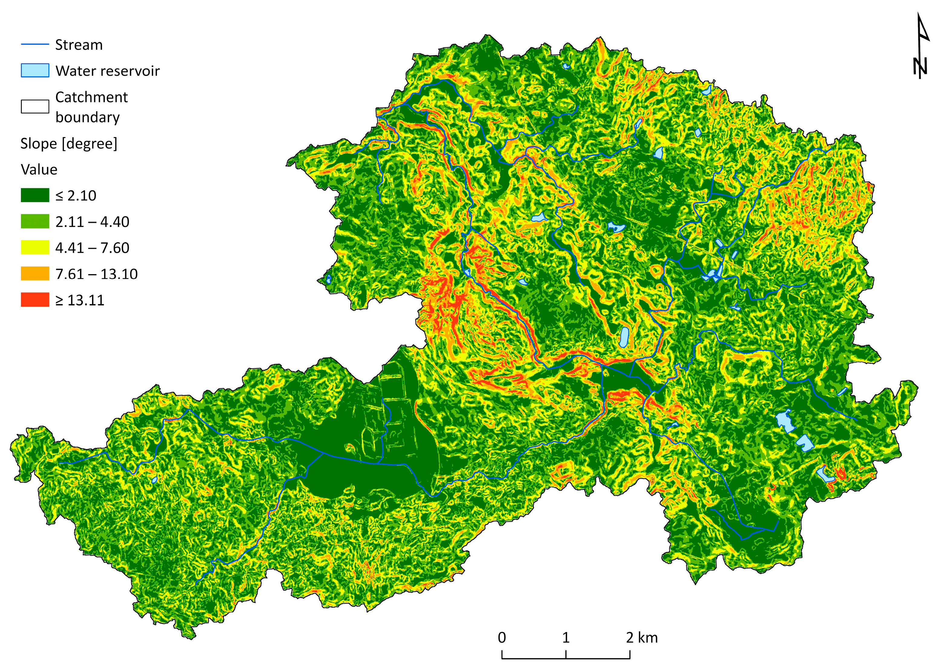
The primary source of topographic information was a Digital Elevation Model (DEM) with a 5 m spatial resolution, obtained from the Head Office of Geodesy and Cartography in Poland (GUGiK), where the base grid resolution is 1 m. DEM was resampled to 5 m prior to SWAT preprocessing, which allowed for a reduction in the number of raster cells used in the calculations while preserving the key characteristics of the terrain morphology. A raster resolution of 5 m is sufficient to generate the correct course of the river network. The DEM was used to delineate catchment boundaries, extract the drainage network, and determine terrain slopes, which were classified into five categories using the Jenks natural breaks method [48] (Figure 2).
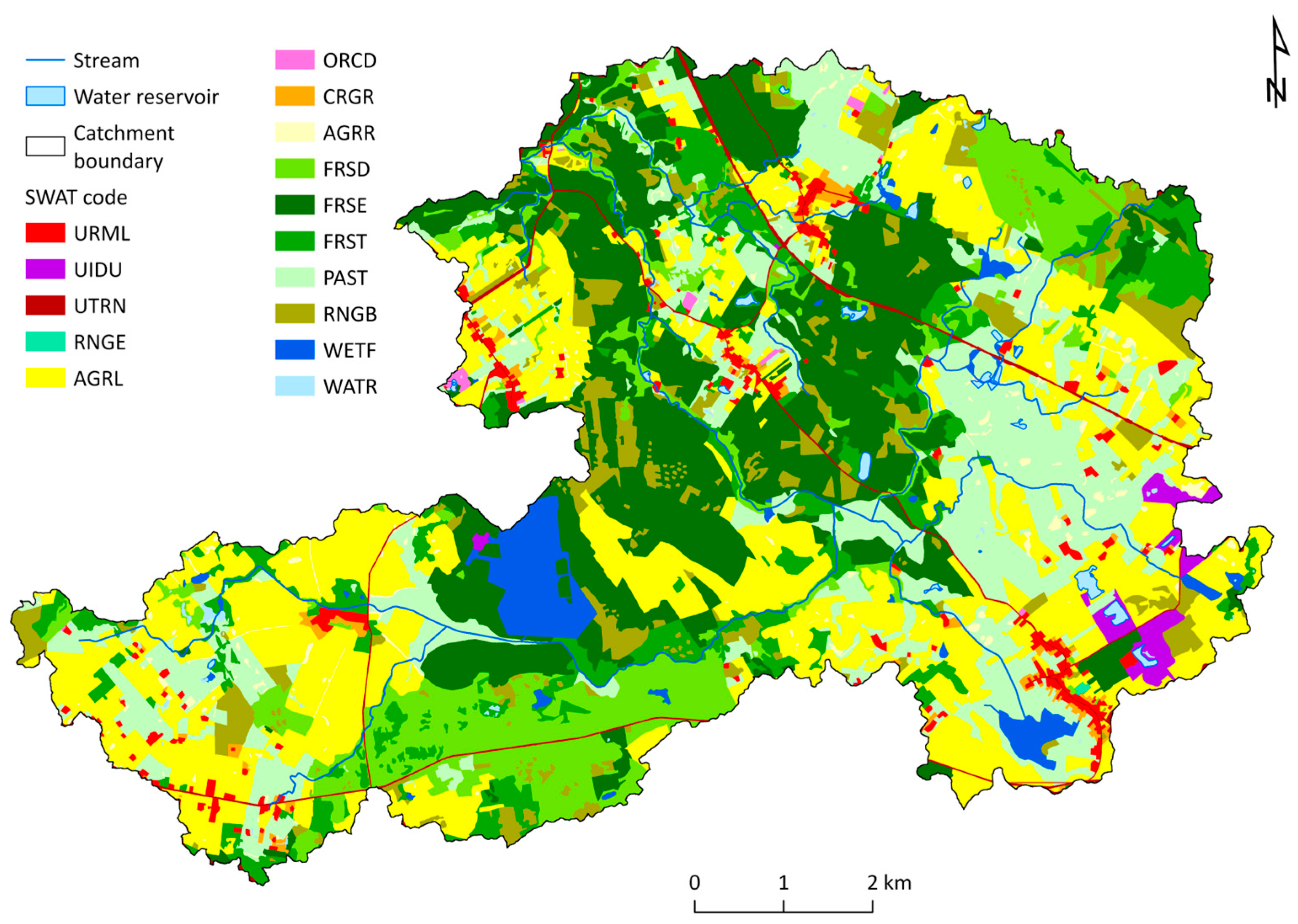
Land use and land cover data were developed at a 1:10,000 scale based on the IMNE datasets, orthophotomaps, and field verification [46]. The development of land cover and land use maps within the IMNE program is based on the CORINE Land Cover classification with minor modifications [49]. The vector layer was converted to a grid layer with a 2 m resolution. This spatial resolution allowed for proper representation of narrow, linear land cover categories, e.g., roads. The IMNE LULC classes were reclassified into the SWAT model categories (Table 2). The major categories included arable land (AGRL) (27%), coniferous forests (FRSE) (20%), natural grasslands (PAST) (18%), broad-leaved forest (FRSD) (10%), and mixed forest (FRST) (7%) (Figure 3). Based on the surface area of individual land cover classes, the average Manning’s roughness coefficient (n) was calculated according to Chow [50], amounting to 0.078 for the catchment area and 0.020 for the stream channel.
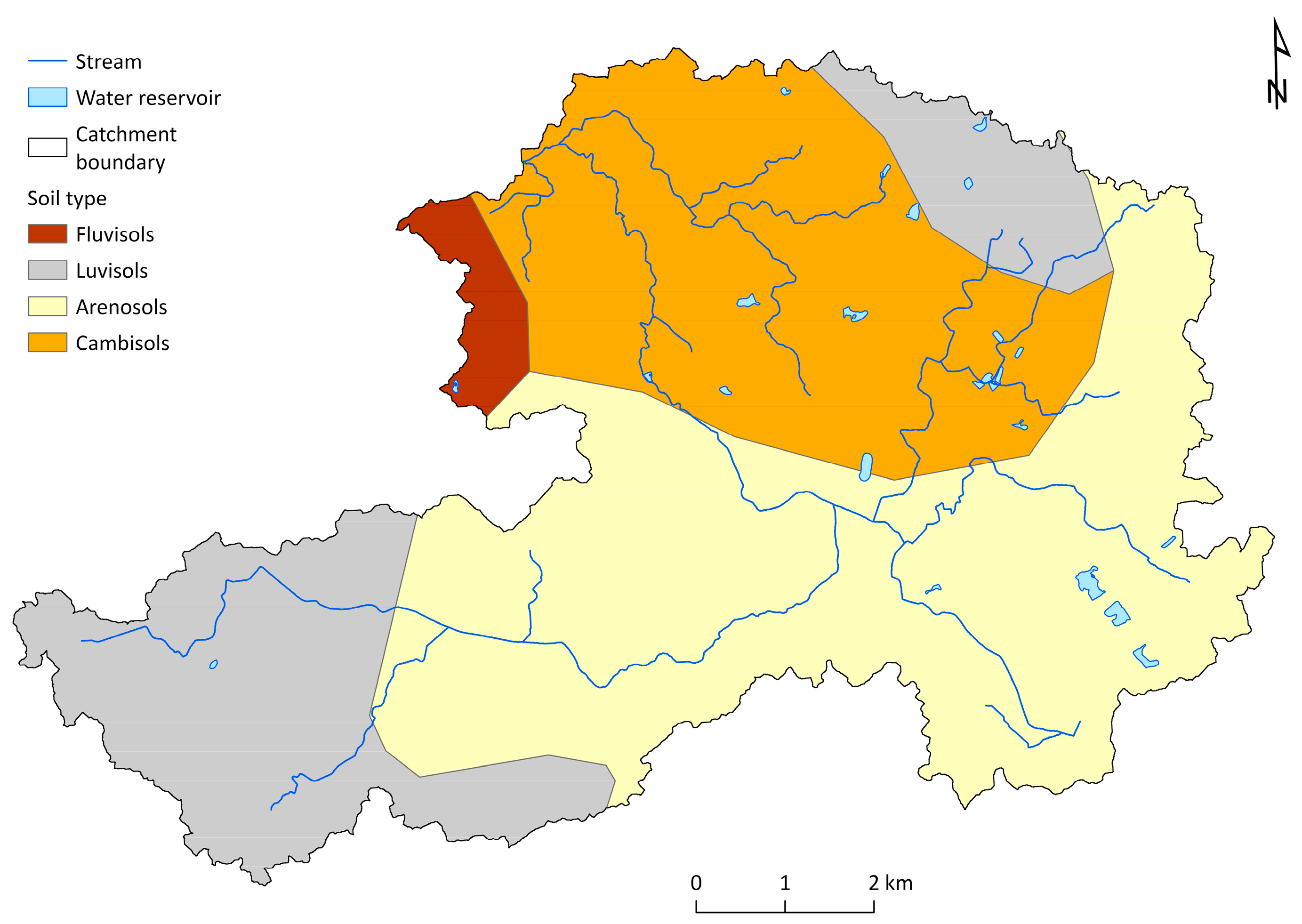
Information about soil properties was obtained from the Harmonized World Soil Database [47], which identifies the dominant soil units in the upper Parsęta basin as Arenosols (46%), Cambisols (27%), Luvisols (23%), and Fluvisols (4%). The HWSD is presented in a low-resolution raster image. Therefore, to spatially map soil types (FAO90), a vector layer from the European Soil Database Maps (ESDAC) was used and converted to a 20 m resolution grid image (Figure 4). Physical soil parameters (e.g., bulk density, available water capacity, hydraulic conductivity, organic carbon content, and texture composition) were implemented in the usersoil table of the SWAT2012.mdb database (Table 3). The soils show spatial variability typical of postglacial lowlands.
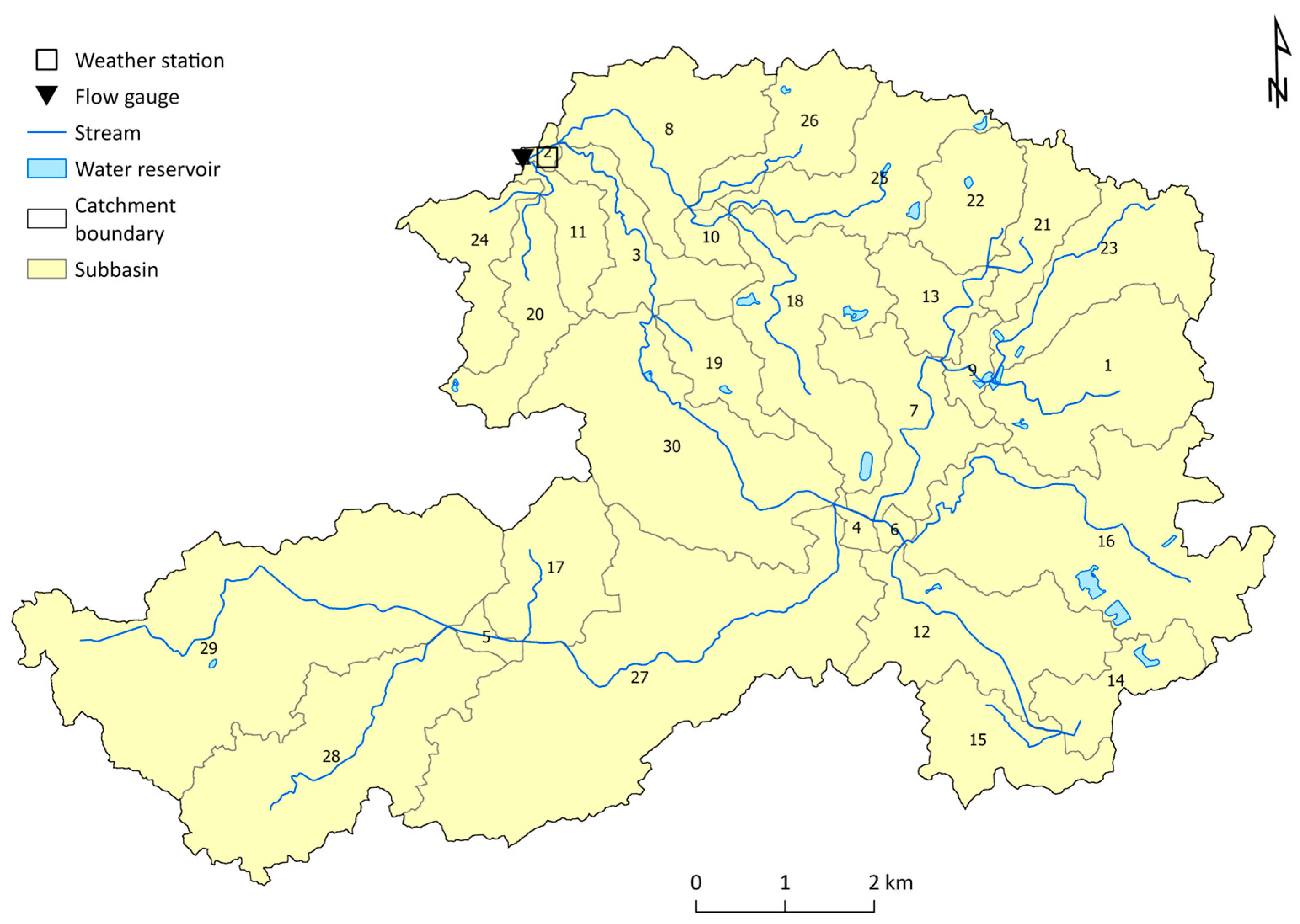
The time series of meteorological and hydrological data originates from measurements conducted within the IMNE monitoring program. The data are collected at a daily time step, and the analyses performed in this study are based on observations from the period 2005–2022. Meteorological data were obtained from the Storkowo meteorological station, located within the study catchment (Figure 1). The observed discharge data originate from a single gauging station (point measurement) located at the catchment outlet (Figure 1) and were used as the reference dataset for model calibration and validation.

2.3. Climate Change Scenarios

Climate data for the periods 2021–2030, 2031–2040, and 2041–2050 were downloaded from the KLIMADA 2.0 portal [51], administered by the Institute of Environmental Protection—National Research Institute (IOS-PIB). The KLIMADA 2.0 database is based on outputs from the EURO-CORDEX initiative, which delivers regional climate simulations downscaled from global CMIP5 climate models. Within the KLIMADA 2.0 framework, these data were further processed using statistical downscaling and bias-correction techniques, ensuring consistency with long-term observations from the Polish meteorological network (Institute of Meteorology and Water Management—National Research Institute, IMGW-PIB) [14,15]. Statistical downscaling based on historical observational data for the reference period 2006–2018 was applied to each model realization, and the corrected projections were extended to 2100. The final projections were derived using an ensemble approach, with the mean of all realizations representing the projected signal and the standard deviation used to quantify projection uncertainty.
The data are provided on a regular grid with a spatial resolution of 0.11° (approximately 12.5 km). The upper Parsęta catchment falls within a grid node of 12.5 × 12.5 km resolution, centered at 16.4431° E and 53.7892° N. The grid point is situated approximately 2 km from the Storkowo meteorological station, ensuring good representativeness of local climatic conditions. For the three decades (2021–2030, 2031–2040, and 2041–2050), monthly mean values of air temperature, total precipitation, relative humidity, and total solar radiation were obtained. The data acquired from the climate scenarios were compiled into databases for the same weather station that was used to run the SWAT model during the calibration and validation periods (Figure 5). The downloaded data include two climate change scenarios:
  • RCP4.5, assuming an increase in the global mean temperature by approximately 2.5 °C by 2100 relative to the pre-industrial conditions;
  • RCP8.5, assuming a global mean temperature rise of about 4.5 °C by 2100 compared to pre-industrial conditions.
These projections enable a detailed assessment of potential changes in thermal and precipitation conditions affecting hydrological processes in the upper Parsęta catchment and are consistent with Poland’s national climate adaptation framework [52].

2.4. Simulation Procedure

The hydrological simulations for the upper Parsęta catchment were carried out using the Soil and Water Assessment Tool model in version SWAT2012 [45]. The input datasets were prepared in ArcGIS software version 9.3.1 with the ArcSWAT extension [53]. The SWAT model was calibrated and validated using the SWAT-CUP (SWAT Calibration and Uncertainty Program) software version 5.1.6 [54].

2.4.1. Catchment Delineation and HRU Definition

The drainage network modeling was performed based on the digital elevation model (DEM). As a result of the catchment delineation, a stream network and subcatchment boundaries were generated, resulting in the delineation of 31 individual subcatchments (Figure 5). Within each subcatchment, the configuration of Hydrologic Response Units (HRUs) was established. The Full HRU option was used, without applying any generalization thresholds, to ensure a detailed spatial representation of land use, soil, and slope variability.

2.4.2. Model Calibration and Validation

After preparation of the input data, the SWAT model was used to simulate the water cycle in the upper Parsęta catchment for the period 2005–2022. Model calibration was performed for the years 2005–2017 (approximately 72% of the observation period) using observed discharge data. Subsequently, the calibrated model was validated for an independent five-year period (2018–2022) representing approximately 28% of the observation period. A sensitivity analysis indicated that the parameters ALPHA_BF, CANMX, CN2, GW_REVAP, LAT_TIME, ESCO, RCHRG_DP, and REVAPMN had the most significant influence on runoff characteristics. The model calibration was conducted in SWAT-CUP 2012 v. 5.1.6 with the SUFI-2 calibration algorithm [54] using monthly discharge data from the Parsęta hydrometric station. The SUFI-2 algorithm [54] aims to identify parameter values that influence the model outputs while providing the smallest possible uncertainty band of the simulations. In SUFI-2, uncertainty represents all sources–input data, model structure, and model parameters–combined into overall simulation (prediction) uncertainty (95PPU). This uncertainty is calculated between the 2.5% and 97.5% levels of the cumulative distribution of the output variable, discarding the 5% poorest simulations. Optimal parameter values were estimated based on the calibration results (Table 4).
Model performance was assessed using statistical coefficients such as Coefficient of Determination (R2), Nash–Sutcliffe Efficiency (NSE), and Percent Bias (PBIAS) [55,56]. The formulas for these metrics are presented below:
R 2 = i = 1 n ( O i O ¯ ) ( P i P ¯ ) i = 1 n ( O i   O ¯ ) 2 i = 1 n ( P i P ¯ ) 2 2
N S E = 1 i = 1 n   ( O i P i ) 2 i = 1 n   ( O i O ¯ ) 2
P B I A S = i = 1 n   O i P i i = 1 n   O i · 100 %
where O is the observed flow, P is the simulated flow, Ō is the average of the observed flow, and P ¯ is the average of the simulated flow.

2.4.3. Scenario-Based Simulations

After the calibration and validation of the SWAT model, flow simulations were performed for the upper Parsęta catchment under two climate scenarios (RCP4.5 and RCP8.5) and three decadal periods: 2021–2030, 2031–2040, and 2041–2050. The climate change scenario data included monthly mean air temperature, total precipitation, relative humidity, and total solar radiation. Data for the three analyzed decades were compared with the reference period 2011–2020. Changes in precipitation, temperature, and water runoff were analyzed as monthly means and for individual seasons. The seasons were defined as follows: DJF—December–January–February; MAM—March–April–May; JJA—June–July–August; SON—September–October–November.

3. Results

This section presents the results in a sequential manner, starting with model performance, followed by projected changes in precipitation and temperature, and finally annual and seasonal runoff responses under both climate scenarios.

3.1. Calibration and Validation Results

The evaluation of the SWAT model performance for the entire study period, including the calibration (2005–2017) and validation (2018–2022) phases, indicates a good representation of the water balance (Table 5). The coefficients of determination (R2) obtained for both the calibration and validation periods demonstrate very good agreement between observed and simulated streamflow. The very low percent bias further confirms the high consistency between measured and simulated values. The model slightly overestimates streamflow during the calibration period and moderately underestimates it during validation. The Nash–Sutcliffe efficiency (NSE) values fall within an acceptable range, indicating that the model adequately captures the streamflow variability across the analyzed periods.
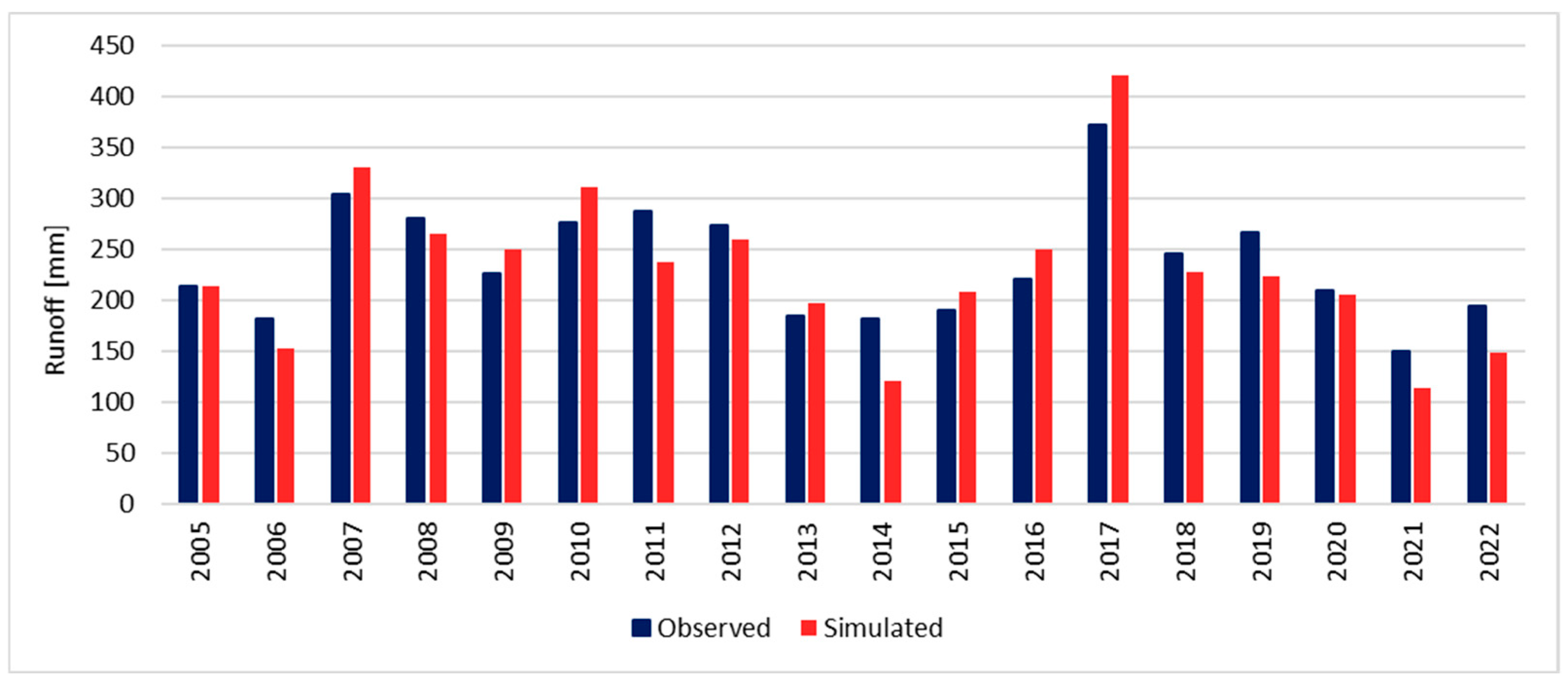
The obtained model evaluation results enable a reliable analysis of runoff based on annual and monthly mean values. Total runoff is composed in SWAT of surface runoff, lateral (sub-surface) flow, and baseflow [16]. The annual observed and simulated runoff totals for 2005–2022 show very good agreement in overall variability and temporal trends (Figure 6). The model accurately reproduces both high- and low-runoff years, effectively capturing the hydrological fluctuations observed throughout the analysis period. The close correspondence between the two time series indicates stable and reliable model performance and its capability to represent the hydrological conditions of the upper Parsęta catchment. The simulated mean runoff for the multi-year period 2005–2022 was underestimated by 3%. The highest underestimation of runoff is observed in 2014, whereas the most pronounced overestimation occurs in 2017.
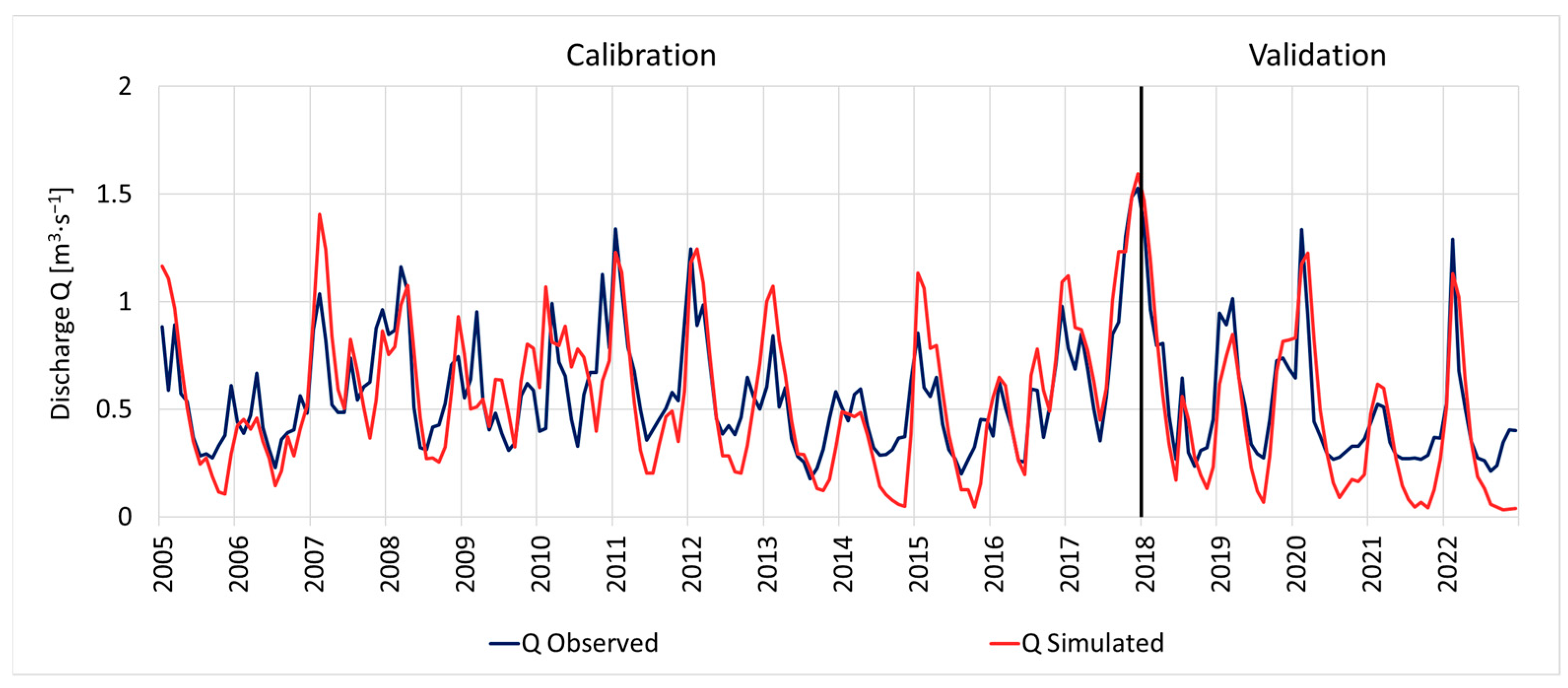
Analyzing the average monthly observed and simulated discharge, it should be noted that the model reliably captures the overall hydrograph pattern and the catchment’s response to varying meteorological conditions (Figure 7). During the calibration period, some peak flows tend to be overestimated, while in the validation period, low-flow conditions are underestimated.
The highest mean monthly runoff from the upper Parsęta catchment occurred during the winter months—January, February, and March—for both observed and simulated values (Table 6). In most months, the simulated runoff values were lower than the observed measurements. The largest percentage differences, about 30%, were recorded in October and November, whereas the smallest differences (<10%) occurred in March, April, May, June, July, and August.

3.2. Projected Precipitation Changes

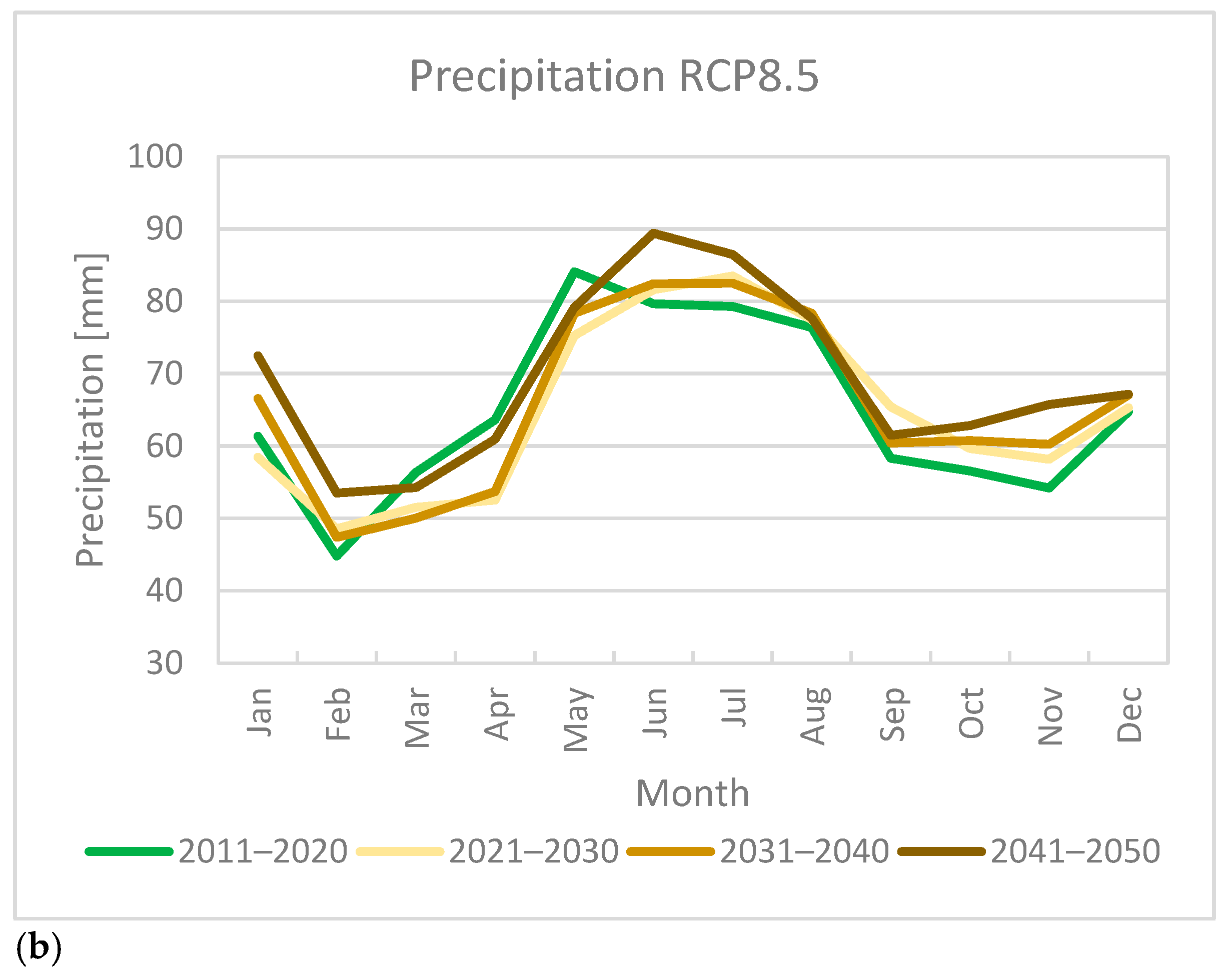
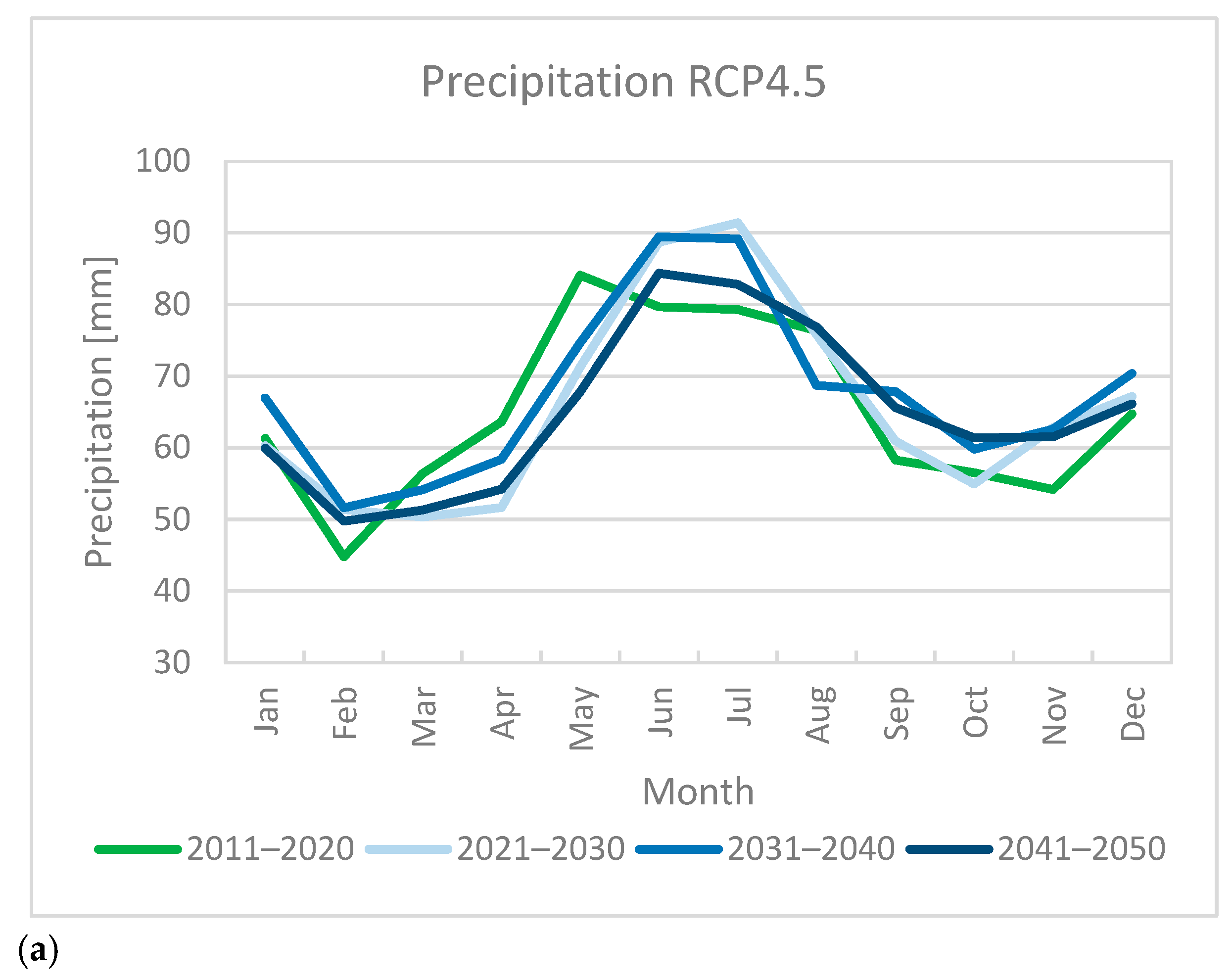
Both scenarios (RCP4.5 and RCP8.5), based on the KLIMADA 2.0 climate model, show pronounced seasonal variability, with increased precipitation projected mainly during the winter (December–February) and autumn (September–November) months (Figure 8). In contrast, spring (March–May) shows a general decline in precipitation relative to the baseline period. The summer season (June to August) is characterized by the highest rainfall. The RCP8.5 scenario exhibits greater amplitude of interdecadal variability than RCP4.5, indicating more pronounced wet and dry anomalies under stronger radiative forcing conditions.
Projections indicate that in the future, precipitation in the upper Parsęta catchment is expected to increase, except during the spring season MAM (March–May), when a decrease in rainfall is projected (Table 7). Precipitation totals will show variability across future decades, with distinct seasonal patterns under both RCP4.5 and RCP8.5 scenarios. The largest relative increase is projected for winter (DJF) and autumn (SON), particularly under the RCP8.5 scenario, where winter precipitation may rise by up to +14% by 2041–2050. Summer (JJA) changes are moderate and relatively stable over decades, ranging from +3% to +9%. In the spring season (March–May), both climate scenarios indicate a consistent decrease in precipitation compared to the historical baseline. The projected reduction ranges from approximately −8% to −15%, suggesting a potential drying trend that may limit soil moisture recharge and early growing-season water availability. These results indicate a shift toward wetter winter–autumn conditions and drier springs, suggesting potential alterations in seasonal water availability and runoff dynamics in the catchment.

3.3. Projected Temperature Changes

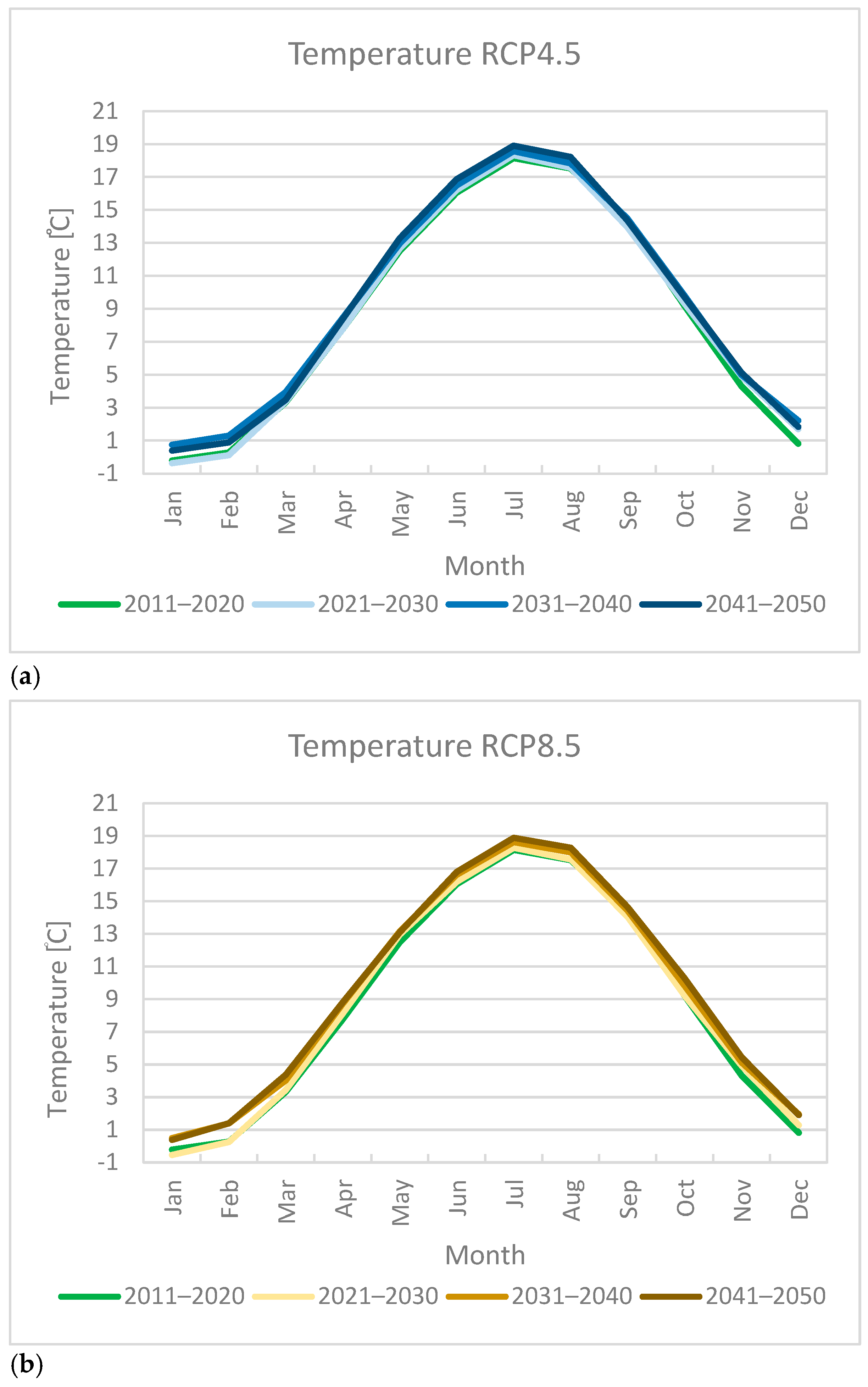
In the historical period, the temperature patterns in the upper Parsęta catchment demonstrate seasonal variation, influencing climatic conditions throughout the year (Figure 9). During the winter months (December to February), temperatures in the basin tend to be cold, with average monthly temperatures ranging from approximately −0.2 °C in January to around +0.8 °C in December. As spring emerges (March to May), temperatures begin to rise, signaling the transition to milder weather. The average monthly temperature during this period ranges from approximately +3.3 °C in March to about +12.5 °C in May, indicating a gradual warming trend. The summer season (June to August) experiences the warmest temperatures, with average monthly temperatures ranging from approximately +16.1 °C in June to +18.2 °C in July. As autumn approaches (September to November), temperatures gradually cool once again. The average monthly temperature during this period ranges from around +14.3 °C in September to approximately +4.3 °C in November, reflecting the transition to cooler weather and the onset of the fall season.
Under both climate scenarios, a gradual increase in mean monthly air temperature is projected throughout the year, with the warming trend intensifying after 2030 (Table 8). Projections based on the KLIMADA 2.0 climate model indicate that, in the 2021–2030 period, the mean annual air temperature is expected to rise by approximately +0.1 °C, and by about +0.6 °C in 2031–2050 under the RCP4.5 scenario, and by around +0.8 °C under RCP8.5. The largest seasonal increase is projected for the winter months (DJF), amounting to +1.1 °C under RCP4.5 and 1.0 °C under RCP8.5, suggesting that future winters may become considerably milder. Overall, both scenarios suggest a continued transition toward warmer climatic conditions in the upper Parsęta catchment, with potential consequences for evapotranspiration rates and runoff dynamics.

3.4. Projected Runoff Changes

The projected mean annual runoff under both climate scenarios (RCP4.5 and RCP8.5) is expected to increase in all three projection decades compared to the reference period (2011–2020) (Table 9). The increase depends on the time horizon and the emission scenario and is most pronounced under the RCP8.5 scenario for the 2041–2050 period. Comparing the individual decades under the RCP4.5 scenario, the mean annual runoff increases systematically in the first two decades (+12.9% in 2021–2030 and +25.5% in 2031–2040), then declines in the third decade, although it still remains higher than in the historical period (+14.5%). Under the RCP8.5 scenario, the mean annual runoff remains close to the reference period in the first two decades (+4.5% in 2021–2030 and +1.1% in 2031–2040), with a significant increase occurring in the third decade (+28.0% in 2041–2050).
To analyze the range of flow variability, the coefficient of variation (Cv) and the irregularity coefficient (α) were calculated (Table 10). The coefficient of variation (Cv) is the ratio of the absolute measure of variability of a feature to the mean value of that feature. The calculations used the standard deviation and the arithmetic mean of the annual mean flows. The irregularity coefficient (α) is the ratio of the maximum to the minimum value of the feature. The calculations were performed based on annual mean flows.
In the reference period 2011–2020, the Cv value of 0.35 and the α value of 4.86 indicate moderate variability in runoff and irregularity between years with the highest and lowest flows (Table 10). This characteristic is typical of small coastal catchments in the lakeland region, where runoff is shaped by a rain–snow regime and relatively high natural retention.
In the climate change projections under the RCP4.5 scenario, a tendency toward gradual stabilization of runoff is observed. In the years 2021–2030, the Cv and α coefficient values slightly decrease, indicating a reduction in the average variability between extreme years. In the following decade (2031–2040), runoff variability reaches its minimum level (Cv = 0.29), and α decreases to 3.23, reflecting the most uniform hydrological regime in the entire analysis. In the years 2041–2050, a slight increase in both indicators is observed, although their values remain lower or comparable to those in the reference period, confirming a general tendency to mitigate runoff fluctuations under the moderate scenario.
A different situation emerges in the high-emission RCP8.5 scenario, where in the first decade of the future period (2021–2030), a decline in runoff stability is observed. The α value reaches the maximum across the entire analysis—up to 5.58—which indicates greater disparities between wet and dry years. This suggests a potential increase in the frequency of extreme events, including hydrological droughts and short-term flood events. In the years 2031–2040, the indicators return to levels comparable to the reference period. In the last analyzed decade (2041–2050), the indicators decreased (Cv = 0.31; α = 3.41), suggesting a stabilization of runoff.
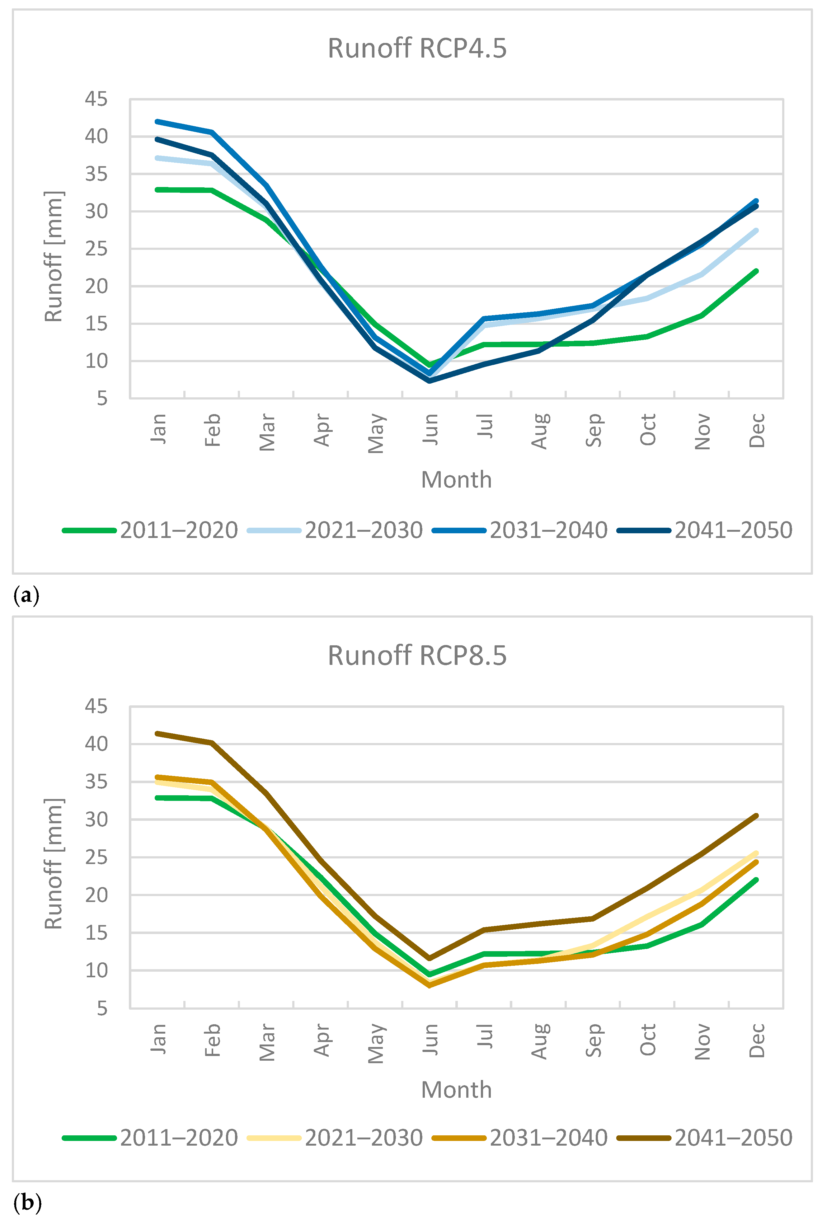
When analyzing monthly runoff changes under both climate scenarios across the three projection decades, an increase in mean runoff relative to the reference period (2011–2020) was observed for most months (Figure 10). In the RCP8.5 scenario, during the 2041–2050 decade, higher runoff values occur in all months of the year. In both scenarios, the simulated streamflow patterns retain a clear seasonal character, with the highest discharges occurring in winter (December–March) and the lowest in summer (May–August). The results indicate an overall increase in runoff throughout most months compared to the historical reference period, particularly pronounced in autumn, reflecting higher projected precipitation. In contrast, a slight reduction in simulated runoff is observed during spring months (April–June), corresponding to the projected decline in precipitation and potential enhancement of evapotranspiration. The seasonal shift in runoff distribution suggests an earlier onset of the high-flow period and a gradual transition toward rainfall-dominated hydrological conditions.
The model correctly reproduces the seasonal runoff pattern observed in the historical data, preserving the characteristic sequence of winter maxima (DJF), summer minima (JJA), and transitional values in spring (MAM) and autumn (SON) (Table 11). Across all decades and scenarios, a general increase in total runoff is projected relative to the baseline period, although the magnitude and timing of changes vary seasonally (Table 11). The highest increases are expected in the autumn (SON) and winter (DJF). Under the RCP4.5 scenario, autumn runoff rises by +5 to +8 mm, while under the RCP8.5 scenario, it rises by +1 to +7 mm. In winter, under the RCP4.5 scenario, the seasonal increases in runoff are the highest among the compared decades, ranging from +4 to +9 mm. Winter runoff also increases substantially, by +2 to +8 mm under RCP8.5, indicating wetter cold seasons associated with higher precipitation and reduced snow accumulation. Spring (MAM) runoff decreases under most scenarios, reflecting lower precipitation and enhanced evapotranspiration during the growing season. For RCP4.5, the reductions are approximately 1 mm, while RCP8.5 shows a similar trend (−1 to −2 mm), except for a slight increase in the 2041–2050 decade. Summer (JJA) projections exhibit greater variability: slight increases (+1 to +2 mm) in the near term (2021–2040) are followed by a decline (−2 mm) under RCP4.5. According to the RCP8.5 scenario, the opposite pattern is observed: a decrease in runoff in the near future (about −1 mm) followed by an increase in the last decade (about +3 mm).
Based on the obtained results, it can be concluded that the answer to the main research question, whether moderate climate forcing (RCP4.5) can generate runoff responses comparable to, or even exceeding, those predicted under extreme forcing (RCP8.5), is affirmative, but only on a seasonal basis. In autumn (SON) and winter (DJF), a greater increase in runoff is projected under moderate climate forcing. In summer (JJA), the moderate scenario will increase runoff, while the extreme scenario will reduce it. The relatively smallest changes will occur in spring (MAM), where both scenarios assume a slight decrease in runoff.

4. Discussion

This section interprets the calibration results and discusses the projected seasonal runoff changes under RCP4.5 and RCP8.5 in relation to precipitation and evapotranspiration patterns. It also addresses key limitations and uncertainties associated with input data and climate projections.

4.1. Discussion of Calibration and Validation Results

The sensitivity analysis showed that the parameters with the most significant influence on runoff generation in the upper Parsęta catchment are the baseflow alpha factor (ALPHA_BF), maximum canopy storage (CANMX), curve number condition II (CN2), groundwater–soil evaporation coefficient (GW_REVAP), lateral flow travel time (LAT_TIME), soil evaporation compensation factor (ESCO), deep aquifer recharge (RCHRG_DP), and the threshold water depth for re-evaporation (REVAPMN). These parameters correspond to the processes that dominate in postglacial lowland catchments, including baseflow contributions, infiltration and soil water retention, and groundwater–surface water interactions. The significant influence of these parameter groups on the simulated water balance in catchments located within the postglacial zone is also confirmed by other studies [57,58]. One of the most important parameters in SWAT simulations is ALPHA_BF, which determines the contribution of groundwater to streamflow. The low value of ALPHA_BF = 0.03 suggests a slow groundwater flow response and a long base-flow recession time, consistent with high natural retention and shallow aquifers typical for sand–clay mosaics of postglacial terrain. Similar values for ALPHA_BF were reported in calibrations for the entire Parsęta river basin [25] and a small lowland catchment in Northern Germany [59].
The obtained R2, NSE, and PBIAS values indicate that the SWAT model adequately reproduces the runoff dynamics in the upper Parsęta catchment. During the calibration period (2005–2017), the coefficient of determination was R2 = 0.66 and the Nash–Sutcliffe efficiency was NSE = 0.43, while in the validation period (2018–2022) the values reached R2 = 0.80 and NSE = 0.59, with very low percent bias (PBIAS: −0.71% in calibration and 13.87% in validation). These results demonstrate good agreement between observed and simulated streamflow, both in temporal variability and total runoff volume. The achieved model performance indicators are comparable to, or higher than, those reported for other lowland catchments [32,60]. According to the hydrological model evaluation guidelines [56], monthly simulations can be considered satisfactory when R2 > 0.6, NSE > 0.50, and PBIAS ≤ 15% for streamflow. In the validation period, the model for the upper Parsęta catchment meets these criteria, whereas during calibration the NSE value is slightly lower (0.43), placing it at the threshold of the range considered acceptable for complex lowland catchments dominated by baseflow. Considering the mosaic character of soil cover, the spatial variability of retention, and the strong interactions between groundwater and surface water, the obtained performance indicators should be viewed as good, particularly in the multi-year perspective.
The model accurately reproduces both high- and low-runoff years, indicating that it correctly captures the influence of precipitation variability and thermal conditions on water availability. The analysis of monthly runoff totals shows that the model reflects the characteristic runoff regime of postglacial rivers in Pomerania, with a winter–spring maximum (January–March) and a summer minimum (June–August). Such a hydrograph pattern has been described for the Parsęta river and other rivers of the coastal and lakeland regions [22], and for lowland catchments in central Poland [61]. The slight overestimation of peak flows and the underestimation of low-flow conditions fall within the range reported for SWAT applications in lowland catchments in Poland and Central Europe [60,62,63], where a high contribution of baseflow and substantial soil water retention increase the model’s sensitivity to uncertainties in input data (precipitation, soil properties, drainage parameters). In summary, the developed model is a reliable tool for analyzing the water balance and the temporal variability of runoff in the upper Parsęta catchment, and it can be applied to assess the effects of projected climate change on future water flows.

4.2. Discussion of Projected Changes in Precipitation, Temperature, and Runoff

The study analyzed projected changes in precipitation and temperature under the RCP4.5 and RCP8.5 scenarios and their effects on runoff in a young-glacial lowland catchment. The projections indicate an overall increase in precipitation across all three future decades in both scenarios. The largest increase (+14%) is expected in the winter season (December–January–February) during 2041–2050 under RCP8.5. A decrease in precipitation is projected only for the spring season (March–April–May). This reduction is particularly pronounced under RCP4.5 in the decades 2021–2030 and 2041–2050. These changes reflect the hydrological consequences of intensified atmospheric circulation and increased moisture availability under warming conditions, which have been identified as major drivers of shifts in the European hydrological cycle [2,3]. They are also consistent with national and regional climate studies for Poland, which report enhanced winter precipitation and a drying tendency in spring [14,15]. The projected rise in air temperature, reaching +0.8 to +1.0 °C under both scenarios, is consistent with expected warming trends in Poland, where the average increase is approximately 1 °C [13]. The projected changes in seasonal mean temperatures indicate a higher winter warming rate than in the other seasons.
Projected changes in precipitation and temperature for the upper Parsęta catchment exhibit patterns consistent with broader tendencies under ongoing climate warming. These trends align with assessments for Poland that highlight a shift toward wetter cold seasons and drier springs, and increasing temperature throughout the year [14,15]. Similar seasonal anomalies are also documented in Europe in regional climate assessments from EURO-CORDEX, with intensifying winter precipitation and enhanced summer evapotranspiration driving changes in runoff regimes [8,12].
This study is based on a widely applied methodology for assessing the impacts of climate change on river flows, combining hydrological modeling with climate change projections [64]. In such studies, a historical period is typically selected as the reference for evaluating future climate change impacts. The study conducted by Liersch et al. [65] emphasized the substantial influence of the chosen baseline period on the interpretation of discharge projections within such a modeling framework. In this work, the reference period was set to 2011–2020. This range is consistent with the historical period adopted in the KLIMADA2.0 project and enables decade-by-decade comparisons of projected runoff changes across three future horizons: 2021–2030, 2031–2040, and 2041–2050.
The interpretation of the modeling results is subject to several sources of uncertainty that should be considered. These uncertainties arise from the quality and spatial resolution of input data, including climate projections, soil data, land-use data, and the digital elevation model. In particular, the coarse resolution of regional climate model outputs relative to the small size of the study catchment limits the explicit representation of spatial climate variability and may affect the simulation of local precipitation and temperature extremes. It should be noted that the climate projections used in this study are derived from the KLIMADA 2.0 database, which provides bias-corrected climate scenarios based on the EURO-CORDEX framework but offers only a single realization per RCP scenario at each grid point. Consequently, the full range of uncertainty associated with the underlying RCM/GCM ensemble spread is not explicitly represented. This limitation precludes a formal quantification of projection uncertainty and implies that the simulated runoff changes should be interpreted as scenario-based signals rather than probabilistic forecasts. Inter-model variability in projected precipitation and temperature—particularly under high-emission scenarios—may therefore lead to a broader range of hydrological responses than those presented here.
The hydrological response simulated by the SWAT model reflects the interplay between climatic drivers. Increases in mean annual runoff are projected across all decades, reaching +13–26% under RCP4.5 and +2–28% under RCP8.5. The most pronounced increase is projected for the decade 2041–2050 under RCP8.5; however, when considering multi-year averages, the RCP4.5 scenario yields greater annual changes. These results may indicate that moderate climate forcing can generate runoff responses comparable to, or in some cases greater than, those projected under extreme forcing; however, this interpretation should be viewed in light of the limited representation of climate model uncertainty inherent to the applied projection dataset. Higher runoff values compared to the historical period are primarily driven by the projected increase in precipitation totals.
In postglacial lowland catchments with high natural retention and strong groundwater–surface water coupling, cold-season precipitation anomalies translate efficiently into runoff because evapotranspiration demand is low and antecedent soil moisture is relatively high. The dominance of baseflow-related parameters in the sensitivity analysis (e.g., ALPHA_BF, GW_REVAP, RCHRG_DP) supports the interpretation that projected runoff changes are primarily mediated by groundwater storage and release rather than by short-lived surface runoff peaks. Although the upper Parsęta catchment represents a small spatial scale, it is representative of postglacial lowlands with groundwater-dominated runoff typical of the southern Baltic region. Thus, the projected directions and seasonal patterns of runoff change are indicative of similar systems. However, the magnitude of changes should be interpreted with caution when transferring the results to larger coastal basins, where scale-dependent processes may alter hydrological responses.
In terms of seasons, the largest increases are projected for autumn and winter. Spring and early summer runoff decreases under most scenarios. The decrease in spring water resources may be associated with rising winter temperatures, which prevent the formation of a persistent snow cover [22]. The melting of snow cover at the end of winter would normally provide recharge to rivers and groundwater. A decreasing trend in snow cover depth is already observed across most of Poland (especially in lowland areas) and in northern Germany [66]. The number of days with snow cover is also decreasing [67]. The projected decrease in runoff from April to June under RCP4.5, and from April to July under RCP8.5, also results from reduced precipitation during this period and from rising air temperatures. Higher air temperatures enhance evaporation from land surfaces, water bodies, vegetation, and other surfaces. Increased evaporation reduces surface runoff and limits water infiltration into the soil, which in turn diminishes groundwater contributions to rivers. The results obtained in this study are similar to findings reported for other catchments in Poland [33,34,38]. For the two lowland catchments–the Barycz and the Upper Narew–Marcinkowski et al. [33] reported an increase in runoff in the near future (2021–2050), with the most pronounced intensification occurring during the winter season. For the largest river basins in Poland (the Vistula and the Odra), SWAT-based projections suggest an increase in mean annual runoff and increases across all seasons in the near future (2021–2050), with the largest changes expected in winter, the smallest in spring, and intermediate, comparable increases in summer and autumn [34]. Winter is the only season in which runoff is projected to rise consistently across all sub-basins and for all RCP-horizon combinations. For spring, the authors noted a spatial divide—relatively stable across scenarios and horizons—where runoff is projected to increase in northern sub-basins and decrease in southern ones. The SWAT model simulations for the Biebrza catchment indicate an increase in average monthly flows in the near future (2024–2050) for nearly all months [38]. The authors identified a slight decrease in mean monthly flow in April and September, while the largest increases are projected for the winter months.
The projected increase in winter and autumn runoff in the upper Parsęta catchment is consistent with findings from other lowland basins in the Baltic Sea region and reflects a broader shift in hydrological regimes under ongoing climate warming. Studies based on SWAT and other process-based hydrological models demonstrate that enhanced cold-season precipitation, combined with pronounced winter warming, leads to a gradual transition from snow-influenced to rainfall-dominated runoff regimes. This transition results in higher winter discharges, reduced snow storage, and a weakening of the traditional spring melt contribution to streamflow [20,68]. In the eastern and northern parts of the Baltic Sea region, similar responses have been attributed to shorter snow cover duration, earlier snowmelt, and an increasing proportion of winter precipitation falling as rain rather than snow, which promotes more direct runoff generation during the cold season.
Comparable seasonal patterns have also been reported for the lowland area in Germany, where increases in winter runoff contrast with reduced flows during summer [69]. These changes are commonly linked to a combination of declining spring precipitation, earlier onset of vegetation activity, and increasing evapotranspiration demand during the growing season, which together limit soil moisture recharge and groundwater replenishment in late spring and summer. As a result, the annual runoff signal becomes increasingly controlled by cold-season conditions, while warm-season flows exhibit greater sensitivity to short-term meteorological variability.
In groundwater-dominated lowland systems, such as postglacial catchments with high natural retention, these seasonal shifts are often accompanied by changes in interannual runoff variability and increased sensitivity to hydrological extremes. Previous SWAT-based studies indicate that under scenarios characterized by stronger climatic forcing, changes in runoff variability may be more pronounced than changes in mean annual discharge, particularly with respect to the contrast between wet and dry years [17]. This behavior is consistent with the results obtained for the upper Parsęta catchment, where elevated irregularity coefficients in the near-term RCP8.5 projections suggest a temporary amplification of interannual variability despite relatively modest changes in mean runoff. Together, these findings indicate that future hydrological change in lowland postglacial catchments will be governed not only by shifts in mean precipitation and temperature, but also by alterations in seasonal runoff distribution and variability, with important implications for water resources management and the frequency of hydrological extremes.

5. Conclusions

This study evaluated the projected impacts of climate change on water runoff in the upper Parsęta catchment—a representative postglacial lowland basin of northwestern Poland—using a calibrated and validated SWAT model. Future climate projections (RCP4.5 and RCP8.5) indicate pronounced seasonal shifts in precipitation and temperature regimes. Both scenarios suggest wetter winters and autumns and a consistent drying tendency in spring, accompanied by a gradual rise in air temperature across all decades. These climatic changes translate into distinct hydrological responses. Simulated runoff increases in most projection periods, with the highest relative changes occurring in autumn and winter, reflecting enhanced cold-season precipitation and reduced snow storage. Conversely, spring flows are expected to decline under most scenarios, in line with decreasing precipitation and increasing evaporative demand. Summer responses show greater variability, depending on the balance between rainfall and evapotranspiration. Together, these projected shifts indicate a transition toward a more rainfall-dominated hydrological regime, with earlier high-flow periods and potential intensification of summer low-flow conditions.
The configured SWAT model for the upper Parsęta catchment is a valid tool for analyzing the water balance and runoff variability. Its good stability and accurate representation of hydrological processes indicate that it can be further used to assess the impacts of land cover and land use changes, and projected climate change, on the runoff regime.

Author Contributions

Conceptualization, M.M., W.B. and J.G.; methodology, M.M., W.B. and J.G.; software, M.M. and W.B.; validation, M.M. and W.B.; formal analysis, M.M. and J.G.; investigation, M.M., W.B. and J.G.; resources, M.M. and J.G.; data curation, M.M. and W.B.; writing—original draft preparation, M.M. and J.G.; writing—review and editing, M.M., W.B. and J.G.; visualization, J.G.; supervision, W.B. All authors have read and agreed to the published version of the manuscript.

Funding

This research received no external funding.

Data Availability Statement

The original contributions presented in this study are included in the article. Further inquiries can be directed to the corresponding author.

Conflicts of Interest

The authors declare no conflicts of interest.

References

  1. Pörtner, H.-O.; Roberts, D.C.; Tignor, M.; Poloczanska, E.S.; Mintenbeck, K.; Alegría, A.; Craig, M.; Langsdorf, S.; Löschke, S.; Möller, V.; et al. (Eds.) Climate Change 2022: Impacts, Adaptation and Vulnerability. Contribution of Working Group II to the Sixth Assessment Report of the Intergovernmental Panel on Climate Change; Cambridge University Press: Cambridge, UK, 2022. [Google Scholar]
  2. Huntington, T.G. Evidence for Intensification of the Global Water Cycle: Review and Synthesis. J. Hydrol. 2006, 319, 83–95. [Google Scholar] [CrossRef] [Scilit]
  3. Gudmundsson, L.; Boulange, J.; Do, H.X.; Gosling, S.N.; Grillakis, M.G.; Koutroulis, A.G.; Leonard, M.; Liu, J.; Müller Schmied, H.; Papadimitriou, L.; et al. Globally Observed Trends in Mean and Extreme River Flow Attributed to Climate Change. Science 2021, 371, 1159–1162. [Google Scholar] [CrossRef] [Scilit] [PubMed]
  4. Teuling, A.J.; de Badts, E.A.G.; Jansen, F.A.; Fuchs, R.; Buitink, J.; Hoek van Dijke, A.J.; Sterling, S.M. Climate Change, Reforestation/Afforestation, and Urbanization Impacts on Evapotranspiration and Streamflow in Europe. Hydrol. Earth Syst. Sci. 2019, 23, 3631–3652. [Google Scholar] [CrossRef] [Scilit]
  5. Blöschl, G.; Hall, J.; Viglione, A.; Perdigão, R.A.P.; Parajka, J.; Merz, B.; Lun, D.; Arheimer, B.; Aronica, G.T.; Bilibashi, A.; et al. Changing Climate Both Increases and Decreases European River Floods. Nature 2019, 573, 108–111. [Google Scholar] [CrossRef] [Scilit] [PubMed]
  6. Eyring, V.; Bony, S.; Meehl, G.A.; Senior, C.A.; Stevens, B.; Stouffer, R.J.; Taylor, K.E. Overview of the Coupled Model Intercomparison Project Phase 6 (CMIP6) experimental design and organization. Geosci. Model Dev. 2016, 9, 1937–1958. [Google Scholar] [CrossRef] [Scilit]
  7. Hausfather, Z.; Peters, G.P. Emissions—The ‘business as usual’ story is misleading. Nature 2020, 577, 618–620. [Google Scholar] [CrossRef] [Scilit]
  8. Jacob, D.; Teichmann, C.; Sobolowski, S.; Katragkou, E.; Anders, I.; Belda, M.; Benestad, R.; Boberg, F.; Buonomo, E.; Cardoso, R.M.; et al. Regional climate downscaling over Europe: Perspectives from the EURO-CORDEX community. Reg. Environ. Change 2020, 20, 51. [Google Scholar] [CrossRef] [Scilit]
  9. Boé, J.; Terray, L.; Martin, E.; Habets, F. Projected Changes in Components of the Hydrological Cycle in French River Basins during the 21st Century. Water Resour. Res. 2009, 45, W08426. [Google Scholar] [CrossRef] [Scilit]
  10. Coppola, E.; Nogherotto, R.; Ciarlo, J.M.; Giorgi, F.; van Meijgaard, E.; Kadygrov, N.; Iles, C.; Corre, L.; Sandstad, M.; Somot, S.; et al. Assessment of the European Climate Projections as Simulated by the Large EURO-CORDEX Regional and Global Climate Model Ensemble. J. Geophys. Res. Atmos. 2021, 126, e2019JD032356. [Google Scholar] [CrossRef] [Scilit]
  11. Anav, A.; Antonelli, M.; Calmanti, S.; Carillo, A.; Catalano, F.; Dell’Aquila, A.; Iacono, R.; Marullo, S.; Napolitano, E.; Palma, M.; et al. Dynamical Downscaling of CMIP6 Scenarios with ENEA-REG: An Impact-Oriented Application for the Med-CORDEX Region. Clim. Dyn. 2024, 62, 3261–3287. [Google Scholar] [CrossRef] [Scilit]
  12. Jacob, D.; Petersen, J.; Eggert, B.; Alias, A.; Christensen, O.B.; Bouwer, L.M.; Braun, A.; Colette, A.; Déqué, M.; Georgievski, G.; et al. EURO-CORDEX: New High-Resolution Climate Change Projections for European Impact Research. Reg. Environ. Change 2014, 14, 563–578. [Google Scholar] [CrossRef] [Scilit]
  13. Mezghani, A.; Dobler, A.; Haugen, J.E.; Benestad, R.E.; Parding, K.M.; Piniewski, M.; Kardel, I.; Kundzewicz, Z.W. CHASE-PL Climate Projection dataset over Poland—Bias adjustment of EURO-CORDEX simulations. Earth Syst. Sci. Data 2017, 9, 905–925. [Google Scholar] [CrossRef] [Scilit]
  14. Struzewska, J.; Jefimow, M.; Jagiełło, P.; Kłeczek, M.; Sattari, A.; Gienibor, A.; Norowski, A.; Dúrka, P.; Walczak, B.; Drzewiecki, P. Zmiany Temperatury i Opadu na Obszarze Polski w Warunkach Przyszłego Klimatu do Roku 2100; Instytut Ochrony Środowiska—Państwowy Instytut Badawczy: Warsaw, Poland, 2020; pp. 1–31. [Google Scholar]
  15. Struzewska, J.; Kaminski, J.W.; Jefimow, M. Changes in Temperature and Precipitation Trends in Selected Polish Cities Based on the Results of Regional EURO-CORDEX Climate Models in the 2030–2050 Horizon. Appl. Sci. 2024, 14, 9. [Google Scholar] [CrossRef] [Scilit]
  16. Arnold, J.G.; Srinivasan, R.; Muttiah, R.S.; Williams, J.R. Large area hydrologic modeling and assessment part I: Model development. J. Am. Water Resour. Assoc. 1998, 34, 73–89. [Google Scholar] [CrossRef] [Scilit]
  17. Huang, S.; Krysanova, V.; Hattermann, F.F. Projections of climate change impacts on floods and droughts in Germany using an ensemble of climate change scenarios. Reg. Environ. Change 2015, 15, 461–473. [Google Scholar] [CrossRef] [Scilit]
  18. Kiesel, J.; Gericke, A.; Rathjens, H.; Wetzig, A.; Kakouei, K.; Jähnig, S.C.; Fohrer, N. Climate Change Impacts on Ecologically Relevant Hydrological Indicators in Three Catchments in Three European Ecoregions. Ecol. Eng. 2019, 127, 404–416. [Google Scholar] [CrossRef] [Scilit]
  19. Leta, O.T.; Bauwens, W. Assessment of the Impact of Climate Change on Daily Extreme Peak and Low Flows of Zenne Basin in Belgium. Hydrology 2018, 5, 38. [Google Scholar] [CrossRef] [Scilit]
  20. Tamm, O.; Maasikamäe, S.; Padari, A.; Tamm, T. Modelling the Effects of Land Use and Climate Change on the Water Resources in the Eastern Baltic Sea Region Using the SWAT Model. CATENA 2018, 167, 78–89. [Google Scholar] [CrossRef] [Scilit]
  21. Plunge, S.; Gudas, M.; Povilaitis, A. Expected Climate Change Impacts on Surface Water Bodies in Lithuania. Ecohydrol. Hydrobiol. 2022, 22, 246–268. [Google Scholar] [CrossRef] [Scilit]
  22. Świątek, M.; Walczakiewicz, S. Changes in Specific Runoff in River Catchments of Western Pomerania versus Climate Change. Geogr. Pol. 2022, 95, 25–52. [Google Scholar] [CrossRef] [Scilit]
  23. Brzozowski, J.; Miatkowski, Z.; Sliwinski, D.; Smarzynska, K.; Smietanka, M. Application of SWAT model to small agricultural catchment in Poland. J. Water Land Dev. 2011, 15, 157–166. [Google Scholar] [CrossRef] [Scilit]
  24. Gudowicz, J. Modelowanie transportu materiału zawieszonego w dorzeczu Parsęty z uwzględnieniem zróżnicowanych rozdzielczości danych przestrzennych. Landf. Anal. 2015, 30, 57–64. [Google Scholar] [CrossRef] [Scilit]
  25. Gudowicz, J.; Zwoliński, Z. Kształtowanie się odpływu rzecznego w dorzeczu Parsęty w świetle modelowania hydrologicznego = Shaping of river outflow in the Parsęta basin in the light of hydrological modelling. Prz. Geogr. 2017, 89, 45–66. [Google Scholar] [CrossRef] [Scilit]
  26. Marcinkowski, P.; Piniewski, M.; Kardel, I.; Srinivasan, R.; Okruszko, T. Challenges in Modelling of Water Quantity and Quality in Two Contrasting Meso-Scale Catchments in Poland. J. Water Land Dev. 2016, 31, 97–111. [Google Scholar] [CrossRef] [Scilit]
  27. Piniewski, M.; Szcześniak, M.; Kardel, I.; Berezowski, T.; Okruszko, T.; Srinivasan, R.; Schuler, D.V.; Kundzewicz, Z.W. Hydrological modelling of the Vistula and Odra river basins using SWAT. Hydrol. Sci. J. 2017, 62, 1266–1289. [Google Scholar] [CrossRef] [Scilit]
  28. Bochenek, W. Prawidłowości Obiegu Wody na Obszarze Beskidzko-Pogórskim Karpat Zachodnich na Przykładzie Zlewni Bystrzanki w Świetle Zmian Klimatu i Działalności Człowieka; Instytut Geografii i Przestrzennego Zagospodarowania PAN: Warsaw, Poland, 2020; Volume 271. [Google Scholar]
  29. Kijowska-Strugała, M.; Bochenek, W. Land Use Changes Impact on Selected Chemical Denudation Element and Components of Water Cycle in Small Mountain Catchment Using SWAT Model. Geomorphology 2023, 435, 108747. [Google Scholar] [CrossRef] [Scilit]
  30. Lach, S.K.; Kopacz, M.T.; Kowalczyk, A.; Grabowska-Polanowska, B. Analysis of Precipitation and Runoff in Carpathian Catchments Using the Soil and Water Assessment Tool Model. J. Ecol. Eng. 2025, 26, 403–415. [Google Scholar] [CrossRef] [Scilit]
  31. Bochenek, W.; Wiejaczka, Ł. Current and future variability of water supply to a mountain reservoir (Polish Carpathians). Stoch. Environ. Res. Risk Assess. 2023, 37, 5051–5069. [Google Scholar] [CrossRef] [Scilit]
  32. Marcinkowski, P.; Kardel, I.; Płaczkowska, E.; Giełczewski, M.; Osuch, P.; Okruszko, T.; Venegas-Cordero, N.; Ignar, S.; Piniewski, M. High-Resolution Simulated Water Balance and Streamflow Data Set for 1951–2020 for the Territory of Poland. Geosci. Data J. 2023, 10, 195–207. [Google Scholar] [CrossRef] [Scilit]
  33. Marcinkowski, P.; Piniewski, M.; Kardel, I.; Szcześniak, M.; Benestad, R.; Srinivasan, R.; Ignar, S.; Okruszko, T. Effect of Climate Change on Hydrology, Sediment and Nutrient Losses in Two Lowland Catchments in Poland. Water 2017, 9, 156. [Google Scholar] [CrossRef] [Scilit]
  34. Piniewski, M.; Szcześniak, M.; Huang, S.; Kundzewicz, Z.W. Projections of Runoff in the Vistula and the Odra River Basins with the Help of the SWAT Model. Hydrol. Res. 2018, 49, 303–317. [Google Scholar] [CrossRef] [Scilit]
  35. Badora, D.; Wawer, R.; Król-Badziak, A.; Nieróbca, A.; Kozyra, J.; Jurga, B. Hydrological Balance in the Vistula Catchment under Future Climates. Water 2023, 15, 4168. [Google Scholar] [CrossRef] [Scilit]
  36. Badora, D.; Wawer, R.; Król-Badziak, A. Modelling 2050 Water Retention Scenarios for Irrigated and Non-Irrigated Crops for Adaptation to Climate Change Using the SWAT Model: The Case of the Bystra Catchment, Poland. Agronomy 2023, 13, 404. [Google Scholar] [CrossRef] [Scilit]
  37. Marcinkowski, P. Projections of Climate Change Impact on Stream Temperature: A National-Scale Assessment for Poland. Appl. Sci. 2024, 14, 10900. [Google Scholar] [CrossRef] [Scilit]
  38. Marcinkowski, P.; Piniewski, M.; Grygoruk, M.; Mirosław-Świątek, D. Climate Change in the Biebrza Basin—Projections and Ecohydrological Implications. Ecohydrol. Hydrobiol. 2024, 24, 796–807. [Google Scholar] [CrossRef] [Scilit]
  39. Majewski, M.; Kostrzewski, A. Stan Geoekosystemów Polski w 2023 Roku na Podstawie Badań Zintegrowanego Monitoringu Środowiska Przyrodniczego; Uniwersytet im. Adama Mickiewicza: Poznan, Poland, 2024. [Google Scholar]
  40. Kostrzewski, A.; Mazurek, M.; Zwoliński, Z. Dynamika Transportu Fluwialnego Górnej Parsęty Jako Odbicie Funkcjonowania Systemu Zlewni; Stowarzyszenie Geomorfologów Polskich: Poznan, Poland; Wydawnictwo Naukowe Bogucki: Poznan, Poland, 1994; pp. 1–165. [Google Scholar]
  41. Karczewski, A. Morfogeneza Strefy Marginalnej Fazy Pomorskiej na Obszarze Lobu Parsęty w Vistulianie (Pomorze Środkowe); Wydawnictwo Naukowe UAM: Poznan, Poland, 1989; pp. 1–48. [Google Scholar]
  42. Piotrowska, I. Struktura użytkowania ziemi w dorzeczu Parsęty. In Funkcjonowanie Geoekosystemów Zlewni Rzecznych. Środowisko Przyrodnicze Dorzecza Parsęty. Stan Badań, Zagospodarowanie, Ochrona; Kostrzewski, A., Ed.; Uniwersytet im. Adama Mickiewicza: Poznan, Poland, 1998; pp. 124–130. [Google Scholar]
  43. Kostrzewski, A. Zintegrowany Monitoring Środowiska Przyrodniczego—Cele, Założenia i Zadania. In Zintegrowany Monitoring Środowiska Przyrodniczego. Propozycje Programowe; Kostrzewski, A., Ed.; Biblioteka Monitoringu Środowiska: Warsaw, Poland, 1995; pp. 7–22. [Google Scholar]
  44. Woś, A. Klimat Polski; Wydawnictwo Naukowe PWN: Warsaw, Poland, 1999. [Google Scholar]
  45. Arnold, J.; Kiniry, J.; Srinivasan, R.; Williams, J.; Haney, E.; Neitsch, S. Soil & Water Assessment Tool: Input/Output Documentation Version 2012; TR-439; Texas Water Resources Institute: College Station, TX, USA, 2012; pp. 1–650.
  46. Szpikowski, J. Zmiany Pokrycia Terenu i Użytkowanie Ziemi. In Raport z Realizacji Programu Badawczo-Pomiarowego Zintegrowanego Monitoringu Środowiska Przyrodniczego w Stacji Bazowej Parsęta w 2022 Roku; Szpikowski, J., Borysiak, J., Domańska, M., Kostrzewski, A., Kruszyk, R., Majewski, M., Szpikowska, G., Eds.; Uniwersytet im. Adama Mickiewicza w Poznaniu: Poznan, Poland, 2023; pp. 176–184. [Google Scholar]
  47. FAO; IIASA; ISRIC; ISSCAS; JRC. Harmonized World Soil Database (Version 1.2); FAO: Rome, Italy; IIASA: Laxenburg, Austria, 2012. [Google Scholar]
  48. Jenks, G.F. The Data Model Concept in Statistical Mapping. Int. Yearb. Cartogr. 1967, 7, 186–190. [Google Scholar]
  49. Zwoliński, Z.; Gudowicz, J. Zmienność przestrzenna typów pokrycia terenu i użytkowania ziemi w zlewniach rzecznych i jeziornych ZMŚP. In Stan i Przemiany Środowiska Przyrodniczego Geoekosystemów Polski w Latach 1994–2015 w Oparciu o Realizację Programu Zintegrowanego Monitoringu Środowiska Przyrodniczego; Kostrzewski, A., Majewski, M., Eds.; Biblioteka Monitoringu Środowiska: Warsaw, Poland, 2018; Volume 32, pp. 491–524. [Google Scholar]
  50. Chow, V.T. Open Channel Flow; McGraw-Hill: New York, NY, USA, 1959; pp. 99–136. [Google Scholar]
  51. Institute of Environmental Protection—National Research Institute (IOS-PIB). KLIMADA 2.0—Climate Change Adaptation Knowledge Platform. Available online: https://klimada2.ios.gov.pl/ (accessed on 10 June 2025).
  52. Ministry of the Environment. Poland’s National Strategy for Adaptation to Climate Change (NAS 2020); Ministry of the Environment: Warsaw, Poland, 2013.
  53. Winchell, M.; Srinivasan, R.; Di Luzio, M.; Arnold, J.G. ArcSWAT 2012: User’s Guide; Blackland Research and Extension Center, Texas A&M AgriLife Research: Temple, TX, USA, 2013.
  54. Abbaspour, K.C. SWAT-CUP 2012, SWAT Calibration and Uncertainty Programs—A User Manual; Eawag: Dübendorf, Switzerland, 2015. [Google Scholar]
  55. Moriasi, D.N.; Arnold, J.G.; van Liew, M.W.; Bingner, R.L.; Harmel, R.D.; Veith, T.L. Model evaluation guidelines for systematic quantification of accuracy in watershed simulations. Trans. ASABE 2007, 50, 885–900. [Google Scholar] [CrossRef] [Scilit]
  56. Moriasi, D.N.; Gitau, M.W.; Pai, N.; Daggupati, P. Hydrologic and water quality models: Performance measures and evaluation criteria. Trans. ASABE 2015, 58, 1763–1785. [Google Scholar] [CrossRef] [Scilit]
  57. Nützmann, G.; Mey, S. Model-Based Estimation of Runoff Changes in a Small Lowland Watershed of North-Eastern Germany. J. Hydrol. 2007, 334, 467–476. [Google Scholar] [CrossRef] [Scilit]
  58. Schmalz, B.; Fohrer, N. Comparing Model Sensitivities of Different Landscapes Using the Ecohydrological SWAT Model. Adv. Geosci. 2009, 21, 91–98. [Google Scholar] [CrossRef] [Scilit]
  59. Wagner, P.D.; Kiesel, J.; Hörmann, G.; Fohrer, N. Representation of Hydrological Processes in a Rural Lowland Catchment in Northern Germany Using SWAT and SWAT+. Hydrol. Process. 2022, 36, e14589. [Google Scholar] [CrossRef] [Scilit]
  60. Piniewski, M.; Okruszko, T. Multi-Site Calibration and Validation of the Hydrological Component of SWAT in a Large Lowland Catchment. In Modelling of Hydrological Processes in the Narew Catchment; Świątek, D., Okruszko, T., Eds.; Geoplanet: Earth and Planetary Sciences; Springer: Berlin/Heidelberg, Germany, 2011; pp. 15–41. [Google Scholar]
  61. Wrzesiński, D. Stability of High and Low Flow Periods on European Rivers. In Badania Fizjograficzne. Seria A—Geografia Fizyczna; Wydawnictwo Poznańskiego Towarzystwa Przyjaciół Nauk: Poznan, Poland, 2015; Volume A66, pp. 183–194. [Google Scholar]
  62. Guse, B.; Reusser, D.E.; Fohrer, N. How to Improve the Representation of Hydrological Processes in SWAT for a Lowland Catchment—Temporal Analysis of Parameter Sensitivity and Model Performance. Hydrol. Process. 2014, 28, 2651–2670. [Google Scholar] [CrossRef] [Scilit]
  63. Pfannerstill, M.; Guse, B.; Fohrer, N. A Multi-Storage Groundwater Concept for the SWAT Model to Emphasize Nonlinear Groundwater Dynamics in Lowland Catchments. Hydrol. Process. 2014, 28, 5599–5612. [Google Scholar] [CrossRef] [Scilit]
  64. Krysanova, V.; Donnelly, C.; Gelfan, A.; Gerten, D.; Arheimer, B.; Hattermann, F.; Kundzewicz, Z.W. How the Performance of Hydrological Models Relates to Credibility of Projections under Climate Change. Hydrol. Sci. J. 2018, 63, 696–720. [Google Scholar] [CrossRef] [Scilit]
  65. Liersch, S.; Drews, M.; Pilz, T.; Salack, S.; Sietz, D.; Aich, V.; Larsen, M.A.D.; Gädeke, A.; Halsnæs, K.; Thiery, W.; et al. One Simulation, Different Conclusions—The Baseline Period Makes the Difference! Environ. Res. Lett. 2020, 15, 104014. [Google Scholar] [CrossRef] [Scilit]
  66. Falarz, M.; Nowosad, M.; Bednorz, E.; Rasmus, S. Review of Polish Contribution to Snow Cover Research (1880–2017). Quaest. Geogr. 2018, 37, 7–22. [Google Scholar] [CrossRef] [Scilit]
  67. Szwed, M.; Pińskwar, I.; Kundzewicz, Z.W.; Graczyk, D.; Mezghani, A. Changes of Snow Cover in Poland. Acta Geophys. 2017, 65, 65–76. [Google Scholar] [CrossRef] [Scilit]
  68. Donnelly, C.; Yang, W.; Dahné, J. River Discharge to the Baltic Sea in a Future Climate. Clim. Change 2014, 122, 157–170. [Google Scholar] [CrossRef] [Scilit]
  69. Middelkoop, H.; Daamen, K.; Gellens, D.; Grabs, W.; Kwadijk, J.C.J.; Lang, H.; Parmet, B.W.A.H.; Schädler, B.; Schulla, J.; Wilke, K. Impact of Climate Change on Hydrological Regimes and Water Resources Management in the Rhine Basin. Clim. Change 2001, 49, 105–128. [Google Scholar] [CrossRef] [Scilit]
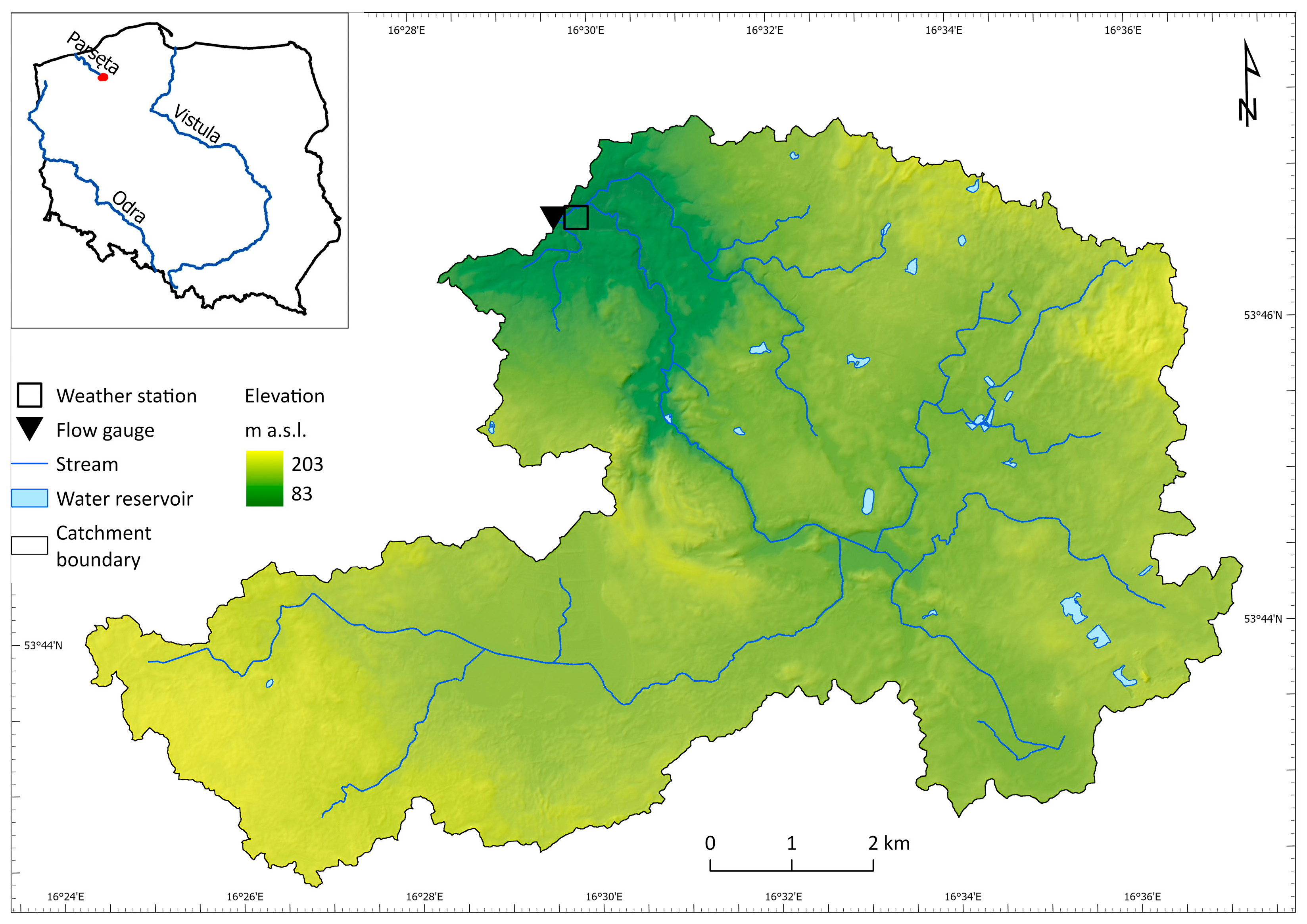
Figure 1. Location of the study area.
Water 18 00419 g001
Figure 2. Slope map of the upper Parsęta catchment.
Water 18 00419 g002
Figure 3. Land Use and Land Cover of the upper Parsęta catchment in 2022.
Water 18 00419 g003
Figure 4. Soil types in the upper Parsęta catchment based on the Harmonized World Soil Database [47].
Water 18 00419 g004
Figure 5. Hydrographic structure of the upper Parsęta catchment.
Water 18 00419 g005
Figure 6. Annual observed and simulated runoff totals for the period 2005–2022.
Water 18 00419 g006
Figure 7. Average monthly observed and simulated discharge (Q) for the calibration and validation periods.
Water 18 00419 g007
Figure 8. Comparison of monthly precipitation totals between historical data (2011–2020) and the two climate scenarios: RCP4.5 (a) and RCP8.5 (b) across three decadal periods: 2021–2030, 2031–2040, and 2041–2050.
Water 18 00419 g008aWater 18 00419 g008b
Figure 9. Comparison of the average monthly air temperatures between historical data (2011–2020) and the two climate scenarios: RCP4.5 (a) and RCP8.5 (b) across three decadal periods: 2021–2030, 2031–2040, and 2041–2050.
Water 18 00419 g009
Figure 10. Comparison of the average monthly flows between historical data (2011–2020) and two climate scenarios: RCP4.5 (a) and RCP8.5 (b) across three decadal periods: 2021–2030, 2031–2040, and 2041–2050.
Water 18 00419 g010
Table 1. Summary of input data used in the SWAT model setup.
Type of DataData SourceSpatial/Temporal ResolutionPeriod or Data Currency
Digital Elevation Model (DEM)Head Office of Geodesy and Cartography (GUGiK)5 m grid2022
Land Use Land Cover[46]2 m grid2022
SoilsHarmonized World Soil Database (HWSD) [47]
European Soil Database Maps (ESDAC)
1 km grid
20 m grid
2012
2001
Weather GeneratorIMNE Parsęta StationMonthly2005–2022
PrecipitationIMNE Parsęta StationDaily2005–2022
Air TemperatureIMNE Parsęta StationDaily2005–2022
Wind SpeedIMNE Parsęta StationDaily2005–2022
Relative HumidityIMNE Parsęta StationDaily2005–2022
Solar RadiationIMNE Parsęta StationDaily2005–2022
DischargeIMNE Parsęta flow gaugeDaily2005–2022
Table 2. Reclassification of CORINE Land Cover (CLC) codes used in the IMNE program into SWAT land use classes.
CLC CodeCLC ClassSWAT CodeSWAT Class
1.1.2Discontinuous urban fabricURMLResidential—Medium/Low Density
1.2.2Road and rail networks and associated landUTRNTransportation
1.3.1Mineral extraction sitesUIDUIndustrial
1.4.1Green urban areasRNGEGrasslands
2.1.1Non-irrigated arable landAGRLAgricultural Land—Generic
2.2.2Fruit trees and berry plantationsORCDOrchards
2.4.2Complex cultivation patternsCRGRCropland/Grassland Mosaic
2.4.3Land principally occupied by agriculture, with significant areas of natural vegetationAGRRCropland/Woodland Mosaic
3.1.1Broad-leaved forestFRSDForest—Deciduous
3.1.2Coniferous forestFRSEForest—Evergreen
3.1.3Mixed forestFRSTForest—Mixed
3.2.1Natural grasslandsPASTPasture
3.2.4Transitional woodland-shrubRNGBShrubland
4.1.2Peat bogsWETFWetlands
5.1.2Water bodiesWATRWater Bodies
Table 3. Physical soil parameters in the upper Parsęta catchment based on the Harmonized World Soil Database [45].
SMU10137101411014210162
FAO 90FluvisolsLuvisolsArenosolsCambisols
HYDGRPDAAB
SOL_ZMX [mm]970800800800
ANION_EXCL [fraction]0.50.50.50.5
SOL_CRK [m3/m3]0.50.50.50.5
SOL_Z [mm]300300300300
SOL_BD [g/m3]1.341.711.71.59
SOL_AWC [mm/mm]0.190.10.10.15
SOL_K [mm/hr]421021061
SOL_CBN [%]2.080.40.50.55
CLAY [%]455510
SILT [%]285610
SAND [%]27908980
ROCK [%]3424
SOL_ALB [fraction]0.210.250.250.24
USLE_K
[t ha h/(MJ mm ha)]
0.32920.180.180.23
Table 4. Optimal calibrated parameter values of the SWAT model in the upper Parsęta catchment.
Parameter NameOptimal Parameter Value
ALPHA_BF0.03
CANMX10
CN240
GW_REVAP0.1
LAT_TIME17
ESCO0.90
RCHRG_DP0.3
REVAPMN400
Table 5. Evaluation of observed and simulated runoff totals based on the following criteria: coefficient of determination (R2), Nash–Sutcliffe efficiency (NSE), and percent bias (PBIAS).
Calibration Period: 2005–2017Validation Period: 2018–2022
R2NSEPBIASR2NSEPBIAS
0.660.43−0.710.800.5913.87
Table 6. Monthly precipitation and runoff depths [mm] in the upper Parsęta catchment for the period 2005–2022.
MonthObserved ValuesSimulated Values
PrecipitationRunoffPrecipitationRunoff
163.627.3663.630.66
239.828.3339.833.60
346.528.1446.530.01
431.722.4631.724.10
568.615.9468.617.03
666.812.3266.812.11
7101.413.68101.412.84
888.713.5988.712.38
955.014.5855.011.84
1038.318.4338.312.09
1161.322.1361.315.71
1260.324.1660.321.68
Table 7. Comparison of seasonal precipitation totals between historical data (2011–2020) and two climate scenarios (RCP4.5 and RCP8.5) across three decadal periods: 2021–2030, 2031–2040, and 2041–2050.
Total Precipitation (Difference Relative to the Reference Period, %)
SeasonRCP4.5RCP8.5
2021–20302031–20402041–20502021–20302031–20402041–2050
DJF5.611.03.71.56.013.8
MAM−14.9−7.8−14.4−12.2−11.2−4.6
JJA8.64.93.73.13.47.7
SON5.912.611.68.37.412.6
Table 8. Comparison of seasonal average monthly air temperatures between historical data (2011–2020) and two climate scenarios (RCP4.5 and RCP8.5) across three decadal periods: 2021–2030, 2031–2040, and 2041–2050.
Air Temperature (Difference Relative to the Reference Period, °C)
SeasonRCP4.5RCP8.5
2021–20302031–20402041–20502021–20302031–20402041–2050
DJF0.21.10.80.01.00.9
MAM0.10.60.50.30.80.9
JJA0.10.40.80.10.50.8
SON0.10.50.50.10.50.9
Table 9. Mean annual runoff for the historical data (2011–2020) and two climate scenarios (RCP4.5 and RCP8.5) across three decadal periods: 2021–2030, 2031–2040, and 2041–2050.
Runoff (mm)
Reference PeriodRCP4.5RCP8.5
2011–20202021–20302031–20402041–20502021–20302031–20402041–2050
229.4259.0288.0262.6239.8232.0293.6
Table 10. Coefficient of variation (Cv) and irregularity coefficient (α) of the mean annual runoff for the historical data (2011–2020) and two climate scenarios (RCP4.5 and RCP8.5) across three decadal periods: 2021–2030, 2031–2040, and 2041–2050.
Coefficient Reference Period RCP4.5 RCP8.5
2011–2020 2021–2030 2031–2040 2041–2050 2021–2030 2031–2040 2041–2050
Cv0.350.340.290.310.360.350.31
α4.864.553.233.515.584.913.41
Table 11. Comparison of the seasonal average monthly runoff between historical data (2011–2020) and two climate scenarios (RCP4.5 and RCP8.5) across three decadal periods: 2021–2030, 2031–2040, and 2041–2050.
SeasonRunoff (mm; Difference Relative to the Reference Period in Parentheses, mm)
Reference PeriodRCP4.5RCP8.5
2011–20202021–20302031–20402041–20502021–20302031–20402041–2050
DJF29.233.7
(+4.4)
38.0
(8.8)
36.0
(6.7)
31.5
(+2.3)
31.6
(+2.4)
37.4
(+8.2)
MAM22.021.0
(−1.0)
23.1
(1.1)
21.2
(−0.8)
21.3
(−0.7)
20.5
(−1.5)
25.1
(+3.1)
JJA11.312.7
(+1.4)
13.4
(2.1)
9.4
(−1.9)
10.1
(−1.2)
10.0
(−1.3)
14.4
(+3.1)
SON13.919.0
(+5.1)
21.5
(7.6)
21.0
(7.1)
17.0
(+3.1)
15.2
(+1.3)
21.1
(+7.2)
Disclaimer/Publisher’s Note: The statements, opinions and data contained in all publications are solely those of the individual author(s) and contributor(s) and not of MDPI and/or the editor(s). MDPI and/or the editor(s) disclaim responsibility for any injury to people or property resulting from any ideas, methods, instructions or products referred to in the content.