Evaluating the Applicability of the wflow_sbm Model with Seamless Parameter Maps for Flood Simulation in Small- and Medium-Sized Catchments

Abstract

Flood simulation in small- and medium-sized catchments is hindered by data scarcity and strong hydroclimatic heterogeneity. Distributed models with pedotransfer functions offer new opportunities, yet their parameter sensitivity and regional applicability remain insufficiently understood. In this study, the wflow_sbm model was applied to two catchments: the humid Tunxi basin and the semi-humid Chenhe basin, China. Model seamless parameters, defined as spatially continuous fields derived directly from global datasets using pedotransfer functions without local calibration, were generated using the HydroMT system. The parameter sensitivity, applicability of pedotransfer function derived parameters, and model performance were systematically evaluated and benchmarked against the well-established Xin’anjiang (XAJ) model, which is a conceptual lumped hydrological model widely used for flood simulation in humid and semi-humid regions of China. Sensitivity analysis identified KsatHorFrac and InfiltCapSoil as dominant in Tunxi, and KsatHorFrac and SoilThickness in Chenhe. SoilThickness derived by HydroMT underestimated flood volumes in the Chenhe basin but was substantially improved after applying a uniform scaling factor of 0.1, resulting in an effective SoilThickness of approximately 0.2 m. The wflow_sbm model achieved performance comparable to the XAJ model. Optimal calibration achieved N_SE = 0.85 in Tunxi with good performance at internal sub-catchments (Yuetan and Chengcun, N_SE > 0.70), and generally above 0.7 in Chenhe. These findings highlight the region-dependent validity of parameterization and provide guidance for distributed flood modeling in data-scarce basins.

1. Introduction

Small- and medium-sized river basins are widely distributed across China and are highly prone to flash floods, debris flows, and other secondary mountain hazards. Hydrological prediction in such basins is particularly challenging due to sparse hydrometeorological observations, strong rainfall variability, and pronounced heterogeneity in land-surface conditions [1]. To address these spatial complexities, distributed hydrological models (DHMs) have shown promising potential. Their parameters possess clearer physical meaning and can better represent the spatial and temporal variability of catchment properties [2,3,4].

Over the past several decades, distributed hydrological modeling has advanced rapidly. Several representative DHMs, such as TOPKAPI [5], VIC [6], WRF-Hydro [7], and wflow_sbm [8], have been widely applied for rainfall–runoff simulation across diverse hydroclimatic regions. These models typically include multiple process options for runoff generation and channel/floodplain routing and can be calibrated using automatic optimization algorithms. A significant trend in their development has been the reduction in calibration dependency through improved parameter estimation. With increasing availability of global datasets [9,10,11], DHMs have progressively adopted parameterization schemes based on soil properties, land-cover characteristics, and topography. This enhances model transferability and provides an important foundation for flood prediction in ungauged or data-scarce basins.

A common approach to assigning parameters to grid cells is through look-up tables (LUTs) that map categorical classes (e.g., soil or vegetation types) to parameter values derived from the literature or land-surface schemes [12,13]. Although computationally simple, LUT-based methods rely on a small number of soil or land-cover classes and often produce discontinuous parameter fields. Pedotransfer functions (PTFs) [14] provide a more continuous alternative by deriving point-scale soil hydraulic parameters from geophysical attributes. However, their empirical nature and scale dependence limit transferability beyond the conditions for which they were developed. To overcome these limitations, recent advances have emphasized spatially continuous and scale-consistent parameterization. Notably, the Multiscale Parameter Regionalization (MPR) framework [15,16] systematically upscales point-scale soil hydraulic information while preserving spatial structure and physical consistency, thereby improving model performance across scales.

The wflow_sbm model [8] developed by Deltares embodies this progression toward flexible and integrated parameterization. It belongs to a family of spatial DHMs that share a common vertical structure based on the Simple Bucket Model (SBM) [17], while allowing flexible representations of lateral flow processes, including overland and channel routing. Owing to this flexible process representation, wflow_sbm is capable of simulating transient catchment runoff dynamics but also involves a large parameter space, with more than 25 potentially tunable parameters, which may complicate model calibration in data-scarce basins. To address this challenge, Imhoff et al. [18] combined PTFs with upscaling techniques to generate seamless, spatially continuous parameter maps and successfully applied them within the wflow_sbm framework. This work led to the development of the HydroMT preprocessing system [19], which enables the automatic construction of model setups and derivation of distributed parameters from globally available datasets. As a result, the number of parameters requiring manual calibration is substantially reduced, making wflow_sbm particularly attractive for applications in ungauged or data-scarce catchments.

Despite these advances, several critical issues remain unresolved when applying seamlessly parameterized distributed models to small- and medium-sized mountainous catchments. First, model sensitivity to parameters is known to vary across catchments as a function of hydroclimatic regime, topography, and land-surface characteristics. In particular, humid and semi-humid regions exhibit distinct runoff generation mechanisms [20]. In humid catchments, runoff is often dominated by saturation-excess processes due to high antecedent soil moisture and shallow water tables, whereas in semi-humid catchments, runoff generation is more strongly controlled by infiltration capacity, soil depth, and subsurface storage, leading to greater event-to-event variability. These fundamental differences imply that the relative importance of model parameters may differ systematically between humid and semi-humid basins, yet whether the wflow_sbm model exhibits such consistent regional differences remains unclear, potentially leading to inefficient calibration. Second, although most wflow_sbm parameters can now be derived automatically from global datasets via PTFs-based approaches, the direct applicability of these parameters across different hydroclimatic regions has not been sufficiently evaluated. Parameters derived from global datasets may not adequately reflect regional characteristics, especially in small- and medium-sized river basins. It remains an open question whether PTF-derived parameters require regional adjustment. Third, while wflow_sbm has been widely applied worldwide, its flood simulation performance in small- and medium-sized basins in China has not been systematically benchmarked against well-established regional models. In humid and semi-humid regions of China, the semi-distributed XAJ model has long served as a reliable reference for rainfall–runoff simulation [21,22,23]. A comparative evaluation against XAJ is therefore essential to objectively assess the performance and practical applicability of wflow_sbm in data-scarce mountainous catchments.

To address these gaps, this study applies the wflow_sbm model to two representative basins in China: the humid Tunxi basin and the semi-humid Chenhe basin. Using HydroMT, distributed parameters are automatically generated based on PTFs and the MPR framework. We (1) systematically analyze the sensitivity of key runoff generation parameters of wflow_sbm model under contrasting hydroclimatic conditions, (2) evaluate the applicability of PTF-derived parameters and examine the necessity of region-specific parameter adjustment, and (3) benchmark the performance of wflow_sbm through comparison with the XAJ model. Multi-site validation is further conducted to assess the spatial robustness of the model. Through these analyses, we aim to clarify the conditions under which seamless parameterization is effective and to provide practical guidance for applying DHMs in data-scarce small- and medium-sized basins.

2. Study Area and Data

2.1. Study Area

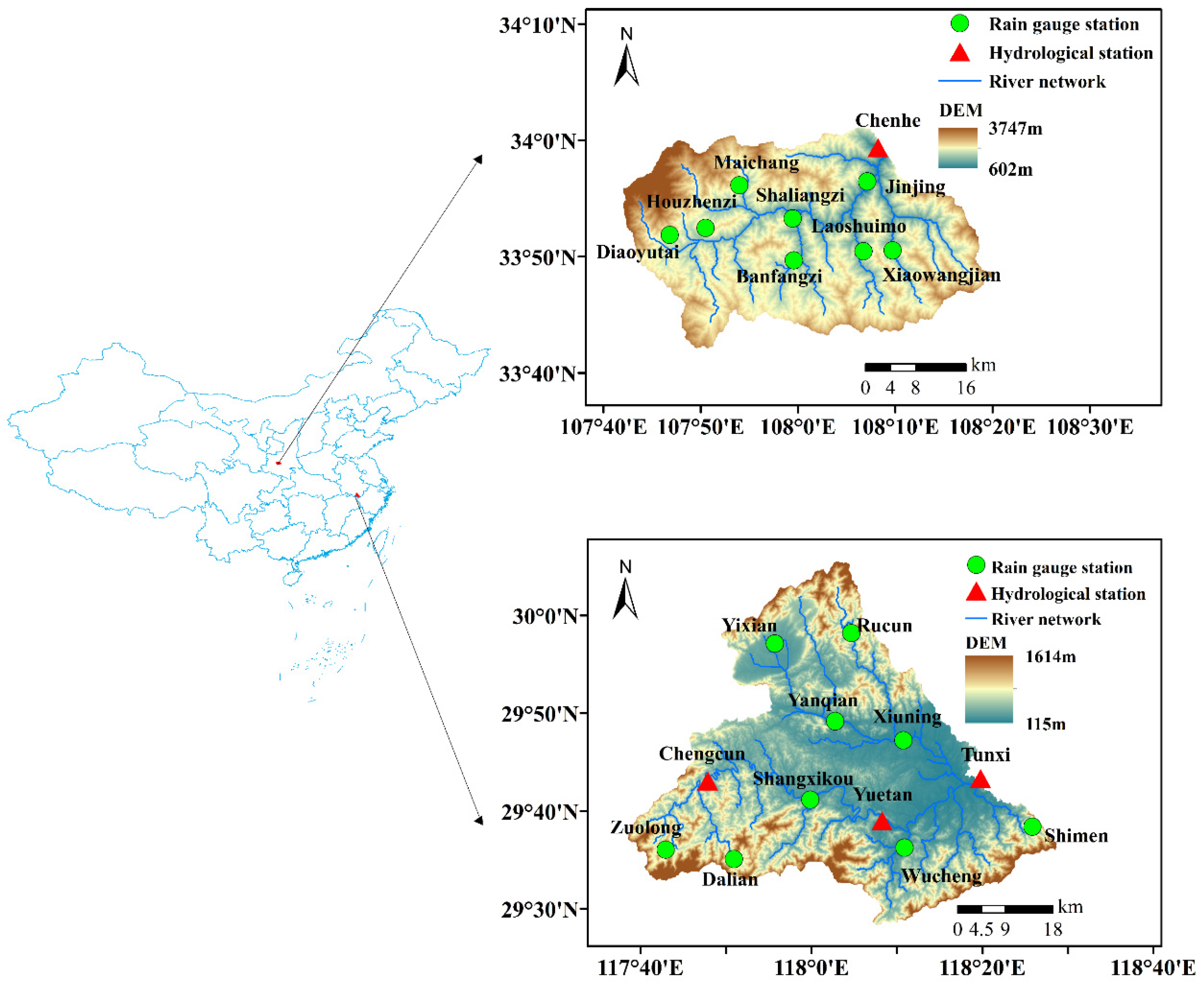
This study focuses on two representative small- and medium-sized catchments in China that exhibit contrasting hydroclimatic and physiographic conditions: the Tunxi catchment in the humid region and the Chenhe catchment in the semi-humid monsoon region of China (Figure 1). The two catchments provide contrasting hydroclimatic regimes for evaluating the adaptability of hydrological models under different climatic and topographic settings.

Tunxi catchment, located in the southern mountainous area of Huangshan City, Anhui Province, has a drainage area of approximately 2692 km². The terrain is steep, with elevations ranging from 115 to 1614 m. The region experiences a humid subtropical monsoon climate, with more than 60% of the annual rainfall occurring during the flood season (May–August). The long-term mean annual precipitation (1982–2002) is about 1600 mm, and streamflow exhibits strong seasonal variability. Discharge observations in the Tunxi catchment are provided by three hydrological stations, including the Tunxi station at the basin outlet and the Yuetan and Chengcun stations located within the interior of the basin. Precipitation data are collected from nine rain gauge stations distributed across the catchment, namely Wucheng, Shimen, Zuolong, Dalian, Shangxikou, Rucun, Yixian, Yanqian, and Xiuning. Chenhe catchment, located in the Weihe Basin in Shanxi Province, has a drainage area of about 1380 km². Elevations vary from 600 m in the lower eastern area to nearly 3700 m in the western mountainous region. The mean annual precipitation (2003–2012) is around 780 mm, most of which occurs during the warm season (June–September). The catchment’s complex topography and spatially variable rainfall make it a suitable representative for semi-humid mountainous catchments in China. In the Chenhe catchment, discharge observations are provided by one hydrological station located at the basin outlet. Precipitation is measured at eight rain gauge stations (Jinjing, Laoshimo, Xiaowangjian, Banfangzi, Shaliangzi, Maichang, Houzhenzi, and Diaoyutai), which are spatially distributed across the basin.

2.2. Available Data

The wflow_sbm model setup and evaluation in this study required three categories of data: geospatial data, meteorological forcing data, and hydrological observations. Geospatial data describe the physical characteristics of the catchments and are used by wflow_sbm to construct the spatially distributed model structure. Meteorological data supply the atmospheric forcing needed to drive the model. Hydrological data serves as independent observations for parameter calibration and performance evaluation. Most geospatial and meteorological datasets were automatically retrieved and preprocessed using the HydroMT framework, which integrates widely used global open-access data sources. Elevation and derived hydrographic information were obtained from the MERIT DEM [24] and the associated MERIT Hydro dataset [9] at 90 m resolution, which provides flow direction, flow accumulation, river networks, and Strahler stream order. Soil properties were derived from the SoilGrids dataset at 250 m resolution [10]. Land-cover information was derived from the ESA CCI land-cover dataset (VITO v2.0.2) [11] at a spatial resolution of 100 m. Precipitation forcing was generated from ground-based measurements. Hourly rainfall records from rain gauge networks within the Tunxi and Chenhe catchments were interpolated to the model grid using inverse distance weighting (IDW). IDW was selected because of its simplicity, numerical stability, and reproducibility, particularly under conditions of limited gauge density. Following common practice in operational hydrological applications, the power parameter of IDW was set to 2 [25]. Temperature and potential evapotranspiration using the de Bruin method [26] were derived based on downscaled ERA5 reanalysis dataset. Streamflow observations at the Tunxi outlet, as well as the interior gauging stations at Yuetan and Chengcun, were used for calibration and multi-site validation during the period 1982–2002. For the Chenhe catchment, discharge data at the basin outlet were used for the period 2003–2012. At all stations, discharge time series were derived from continuously recorded water stage measurements and established stage–discharge rating curves at each station. The rating curves were developed and periodically updated by the hydrological authorities through routine current-meter measurements. To meet the temporal requirement of flood simulation, the discharge series were interpolated to 1 h resolution using linear interpolation between successive records.

The XAJ model relies primarily on rain gauge observations and pan-evaporation measurements as its forcing inputs. For both the Chenhe and Tunxi catchments, pan-evaporation observations from nearby meteorological stations were employed and subsequently transformed into basin-scale potential evaporation to provide consistent inputs for both models.

3. Methods

3.1. The wflow_sbm Model and Parameterization

The conceptual bucket model wflow_sbm is based on topog_sbm with a kinematic-wave approach for lateral subsurface, overland and river flow routing, and the local inertial method for overland and river flow routing. It has four main routines: (i) a precipitation–snow routine based on the HBV model [27], (ii) a rainfall interception routine based on the modified Rutter model [28] or Gash model [29], (iii) a soil water routine based on topog_sbm, and (iv) a flow generation routine with the kinematic-wave and local inertial method.

In the wflow_sbm model, infiltration is partitioned into compacted and non-compacted fractions of each grid cell, controlled by soil and land-use properties. For each fraction, the maximum infiltration rate is defined as the minimum of the soil infiltration capacity (InfiltCapSoil) and the incoming water flux. Overland flow is generated through infiltration-excess runoff when rainfall intensity exceeds InfiltCapSoil.

The soil is considered as a bucket with a finite soil depth (SoilThickness), divided into a saturated store and an unsaturated store. All infiltrating water enters the unsaturated store first. The soil bucket can be split up into different layers. Assuming a unit head gradient, the potential transfer of water $Q_{transfer,pot,n}$ from an unsaturated layer is controlled by the vertical saturated hydraulic conductivity $K_{vz,n}$, the effective saturation degree of layer n, and a Brooks–Corey power coefficient $c_n$ based on the pore size distribution index ${\lambda }_n$ of layer n [30]. The soil water routine assumes an exponential decay of the saturated hydraulic conductivity with soil depth [31]:

$$Q_{transfer,pot,n}=K_{vz,n}{\left({\displaystyle \frac{{\theta }_n-{\theta }_r}{{\theta }_s-{\theta }_r}}\right)}^{c_n}$$

(1)

$$c_n={\displaystyle \frac{2+3{\lambda }_n}{{\lambda }_n}}$$

(2)

where ${\theta }_n$ is the soil water content of unsaturated soil layer n and ${\theta }_s$ and ${\theta }_r$ (thetaS and thetaR) are the saturated and residual soil water contents, respectively.

Lateral subsurface flow is represented using a kinematic-wave approximation, which describes the downslope transport of soil water above the water table. The kinematic-wave equation is solved iteratively using the Newton–Raphson method. If the entire soil column becomes saturated, saturation-excess overland flow is triggered, and exfiltration from the soil surface is calculated accordingly.

The governing equation for subsurface discharge $Q_{subsurface}$ along the flow path is

$${\displaystyle \frac{\partial Q_{subsurface}}{\partial t}}=-c{\displaystyle \frac{\partial Q_{subsurface}}{\partial x}}+cw{R}_{input}$$

(3)

where $t$ is time, $x$ is the downslope distance (m), $w$ is the effective flow width of the grid cell (m), and $R_{input}$ is the net input rate to the saturated zone ($\mathrm{m}{\mathrm{s}}^{-1}$). It represents the balance between vertical recharge from the overlying unsaturated soil layers and losses from the saturated store. Specifically, $R_{input}$ consists of the actual vertical transfer of soil water $Q_{transfer,pot,n}$ from unsaturated layer n above the water table at the previous time step, minus losses due to capillary rise, transpiration from the saturated zone, leakage, and soil evaporation from the saturated store.

The wave celerity $c$ controls the propagation speed of lateral subsurface flow and is defined as

$$c={\displaystyle \frac{K_{h0}exp\left(f_{ssf}{K}_v{z}_{ssf,watertable}\right)c_{landslope}}{{\theta }_s-{\theta }_r}}$$

(4)

where $K_v$ is the vertical saturated hydraulic conductivity($\mathrm{m}{\mathrm{s}}^{-1}$), $z_{ssf,watertable}$ is the depth to the water table (m), $K_{h0}$ is the saturated horizontal hydraulic conductivity at the soil surface ($\mathrm{m}{\mathrm{s}}^{-1}$), which is derived by scaling the vertical saturated hydraulic conductivity using a dimensionless fraction parameter (KsatHorFrac), $f_{ssf}$ is a decay parameter controlling the exponential decrease in hydraulic conductivity with soil depth (${\mathrm{m}}^{-1}$), and $c_{landslope}$ is the local land-surface slope.

Overland and river flow were simulated also using the kinematic-wave approximation. The kinematic-wave equations are nonlinear, and the model solves them iteratively using the Newton–Raphson method. Here, the default fixed internal timestep is 900 s for river cells and 3600 s for overland cells.

$${\displaystyle \frac{\partial Q}{\partial x}}+\alpha \beta Q^{\beta -1}{\displaystyle \frac{\partial Q}{\partial t}}=q_{inflow}$$

(5)

where $Q$ is the surface flow in the kinematic wave (m³ s⁻¹), $x$ is the length of the flow pathway (m), $q_{inflow}$ is the lateral inflow per unit length into the kinematic wave (m² s⁻¹), $t$ is the integration timestep, and $\alpha$ and $\beta$ are coefficients. These coefficients can be determined by using Manning’s equation [32].

Flood simulations were performed using the wflow_sbm model (version 0.6.3). The model was built using the HydroMT-Wflow plugin (version 0.8.0). All forcing and static data sources used in this study are described in Section 2.2. The main parameters and their sources for global parameterization used in this study are indicated in

Table 1. Main wflow_sbm parameters and their sources for global parameterization.

Model Parameter	Description	Parameterization
c	Power coefficient based on the pore size distribution index used for computing vertical unsaturated flow (–)	Rawls and Brakensiek (1989) [33]
Kext	Extinction coefficient in the canopy gap fraction equation (–)	Van Dijk and Bruijnzeel (2001) [34]
KsatVer	Vertical saturated conductivity (mm day−1)	Brakensiek et al. (1984) [35]
LAI	Long-term monthly average leaf-area index (–)	Myneni et al. (2015) [36]
M	Decay rate of KsatVer with depth (mm)	Derived as exponential decay function from KsatVer at seven depths
N	Manning’s roughness coefficient for the kinematic-wave function for overland flow (m−1/3 s)	Engman (1986) [37] and Kilgore (1997) [38]
N_River	Manning’s roughness coefficient for the kinematic-wave function for river flow (m−1/3 s)	Liu et al. (2005) [39]
RootingDepth	Maximum length of vegetation roots	Fan et al. (2016) [40] and Schenk and Jackson (2002) [41]
SI	Specific leaf storage for the interception module (mm)	Pitman (1989) [42] and Liu (1998) [43]
Slope	Slope (–)	Farr et al. (2007) [44]
SoilThickness	Depth of the upper aquifer (mm)	Hengl et al. (2017) [10]
Swood	Fraction of wood in the vegetation (–)	Pitman (1989) [42] and Liu (1998) [43]
thetaR	Residual water content (–)	Tóth et al. (2015) [45]
thetaS	Saturated water content (–)	Tóth et al. (2015) [45]
RiverWidth	River width (mm)	Leopold et al. (1953) [46]
RiverDepth	River depth (mm)	Leopold et al. (1953) [46]
KsatHorFrac	Multiplication factor applied to KsatVer for the horizontal saturated conductivity used for computing the lateral subsurface flow (–)	Calibration
InfiltCapSoil	Infiltration capacity of the non-compacted soil (mm day−1)	Default 100

. The model resolution was set to 1 km, resulting in 3629 grid cells in the Tunxi basin and 1958 grid cells in the Chenhe basin.

3.2. Key Parameter Sensitivity Analysis

To evaluate the sensitivity differences in key runoff generation parameters between humid and semi-humid regions, this study selected three parameters—KsatHorFrac, InfiltCapSoil, and SoilThickness—and conducted a sensitivity analysis in the Tunxi and Chenhe catchments. Two representative flood events were selected: the 26 August 1984 flood in Tunxi and the 3 September 2003 flood in Chenhe. Each parameter was systematically varied within physically reasonable ranges, while others were held constant. The parameter ranges (

Table 2. Parameter settings for sensitivity analysis.

Parameter	Constant Value	Tested Values
KsatHorFrac	100	1, 3, 10, 30, 100, 300, 500, 800, 1000, 3000, 5000, 8000, 10,000
InfiltCapSoil	100	10, 20, 40, 80, 100, 120, 200, 400, 800, 1200, 1600, 2500
SoilThickness	HydroMT (about 2 m)	* 0.1, * 0.25, * 0.5, * 0.75, * 1.0

Note: * indicates a multiplier relative to the default SoilThickness value derived from HydroMT.

) were determined based on Imhoff et al. [18]. Initial spatially distributed SoilThickness fields were obtained from the HydroMT parameterization scheme, with maximum depths of up to 2 m across the basin. From these initial values, uniform scaling factors (0.1–1.0) were applied to assess the parameter’s catchment-wide sensitivity. KsatHorFrac and InfiltCapSoil were treated as spatially uniform parameters during the sensitivity analysis, with a series of fixed values tested to quantify their influence on model performance.

Model outputs were evaluated using three performance metrics: the relative runoff error (PB), Nash–Sutcliffe efficiency (NSE), and Kling–Gupta efficiency (KGE) [47]:

$$\mathrm{P}\mathrm{B}={\displaystyle \frac{\overline{Q_{sim}}-\overline{Q_{obs}}}{\overline{Q_{obs}}}}\times 100\mathrm{\%}$$

(6)

$$\mathrm{N}\mathrm{S}\mathrm{E}=1-{\displaystyle \frac{\sum _{t=1}^z{\left(Q_{sim}^t-Q_{obs}^t\right)}^2}{\sum _{t=1}^z{\left(Q_{obs}^t-\overline{Q_{obs}}\right)}^2}}$$

(7)

$$\mathrm{K}\mathrm{G}\mathrm{E}=1-\sqrt{{\left(R-1\right)}^2+{\left(\alpha -1\right)}^2+{\left(\beta -1\right)}^2}$$

(8)

Here, $Q_{obs}$ and $Q_{sim}$ represent the observed and simulated discharge series, respectively. $R$, $\alpha$, and $\beta$ denote the correlation coefficient, the ratio of standard deviations, and the ratio of means between observed and simulated discharge. The relative bias PB emphasizes the overall water balance between the simulated and observed streamflow, where PB = 0 indicates perfect volume agreement. The NSE focuses on the model’s ability to reproduce the temporal dynamics of the hydrograph. The KGE integrates information from correlation, bias, and variability to provide a balanced assessment of model performance. Higher NSE and KGE values indicate better model performance.

3.3. wflow_sbm Model Calibration and Evaluation

For the wflow_sbm model, a manual trial-and-error calibration approach was adopted, guided by the parameter sensitivity analysis presented in Section 3.2. The calibration focused on three key parameters identified as most sensitive: KsatHorFrac, InfiltCapSoil, and SoilThickness. For Tunxi, 33 flood events were used, including 22 for calibration and 11 for validation. For Chenhe, 20 flood events were selected, with 13 for calibration and 7 for validation. Each simulation included a five-month warm-up period prior to the first event to ensure proper initialization. Model performance was evaluated using four indicators following the Ministry of Water Resources of China standard [48]: the four metrics were chosen as evaluation criteria including relative runoff volume error ($E_{RR}$, %), relative peak discharge error ($E_{RP}$, %), peak time error ($E_{PT}$, h), and Nash–Sutcliffe efficiency ($N_{SE}$):

$$E_{RR}={\displaystyle \frac{R_{sim}-R_{obs}}{R_{obs}}}\times 100\mathrm{\%}$$

(9)

$$E_{RP}={\displaystyle \frac{Q_{peak,sim}-Q_{peak,obs}}{Q_{peak,obs}}}\times 100\mathrm{\%}$$

(10)

$$E_{PT}=T_{peak,sim}-T_{peak,obs}$$

(11)

$$N_{SE}=1-{\displaystyle \frac{\sum _{t=1}^z{\left(Q_{sim}^t-Q_{obs}^t\right)}^2}{\sum _{t=1}^z{\left(Q_{obs}^t-\overline{Q_{obs}}\right)}^2}}$$

(12)

where $R_{obs}$ is the observed runoff volume; $R_{sim}$ is the simulated runoff volume; $Q_{peak,sim}$ is the observed peak discharge; $Q_{peak,obs}$ is the simulated peak discharge; $T_{peak,obs}$ is the observed time of flood peak; $T_{peak,sim}$ is the simulated time of flood peak; $Q_{obs}^t$ is the observed discharge for each time step t; $Q_{sim}^t$ is the simulated or predicted value at time $t$; $\overline{Q_{obs}}$ is the observed mean within the time period of analysis; and $z$ is the total number of values. A simulation is regarded as a qualified simulation regarding total runoff volume error if the absolute value of $E_{RR}$ is less than 20%. If the absolute value of $E_{RP}$ is less than 20%, this simulation is regarded as a qualified simulation regarding peak discharge error. Similarly, if the absolute value of $E_{PT}$ is within 3 h, this simulation is regarded as a qualified simulation regarding peak time error; if the $N_{SE}$ is greater than 0.7, this simulation is regarded as a qualified simulation regarding goodness of fit.

The primary objective during manual calibration was to jointly maximize $N_{SE}$ and while minimizing $E_{RR}$, $E_{RP}$, and $E_{PT}$. To evaluate the internal spatial consistency of the wflow_sbm model, the parameters calibrated at the Tunxi outlet were directly applied to the upstream sub-catchments draining to the Chengcun and Yuetan stations. Simulations at these interior gauges were then validated without any further parameter adjustment, serving as a rigorous test of model transferability.

3.4. XAJ Model Description and Setup

For comparison, the XAJ model was implemented in both catchments to benchmark the performance of the wflow_sbm model. Although both models are conceptual, they differ substantially in their levels of spatial representation and model structural complexity. The XAJ model adopts a semi-distributed framework, in which sub-catchments delineated according to rain gauge distribution serve as the basic computational units. Runoff generation in XAJ is based on a saturation-excess mechanism, whereby runoff is produced once soil moisture storage reaches field capacity. Spatial heterogeneity in soil water storage is represented using two conceptual storage capacity curves: a tension water storage capacity curve and a free water storage capacity curve. Soil moisture is partitioned into tension water and free water, controlled by the parameters WM (maximum tension water storage capacity) and SM (free water storage capacity), respectively. The parameter WM primarily governs soil moisture dynamics and runoff generation, whereas SM determines the partitioning of total runoff into surface runoff, interflow, and groundwater flow. Runoff generated within each sub-catchment is routed to the catchment outlet through a two-stage procedure. First, runoff is transferred to the sub-catchment outlet using a lag-and-route method, in which the recession parameter Cs plays a critical role in controlling flood peak magnitude [1]. Subsequently, channel routing is performed using the Muskingum successive-reaches method. A comprehensive description of the XAJ model can be found in Zhao [49]. Model parameters were calibrated using the Shuffled Complex Evolution global optimization algorithm (SCE-UA) [50] based on outlet discharge. The same set of flood events as used for the wflow_sbm model was employed for both calibration and validation. The calibrated values of the key parameters for the Tunxi and Chenhe catchments are listed in

Table 3. Parameters and their physical meaning.

Parameter	Description	Value of Tunxi	Value of Chenhe
Ke	Ratio of potential evapotranspiration to pan-evaporation	1.1	0.8
WM	Tension water capacity (mm)	120	180
SM	Free water capacity (mm)	15	10
CS	Recession constant in the lag-and-route method	0.9	0.06

.

4. Results

4.1. Sensitivity of Key Parameters and Model Calibration

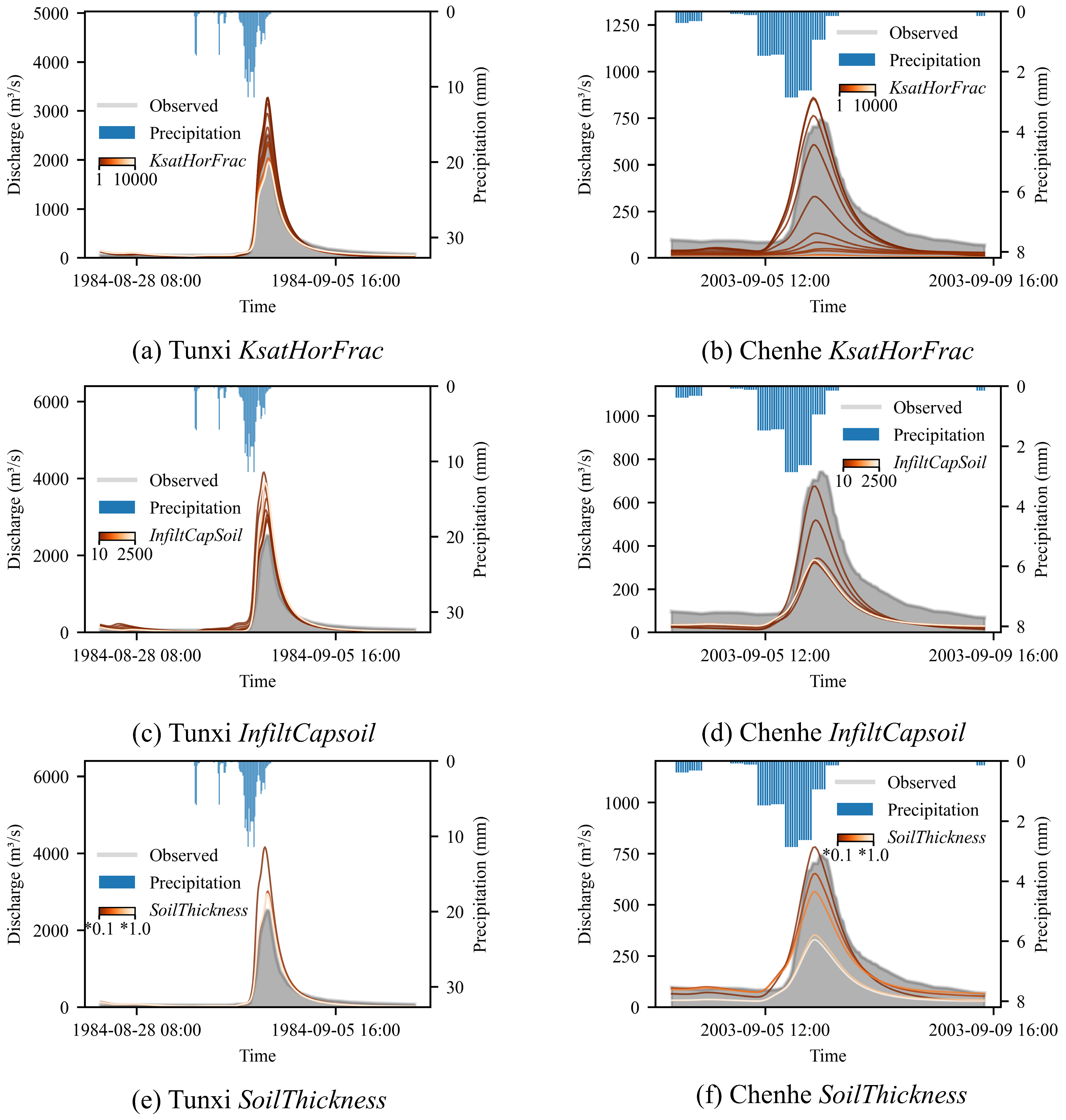
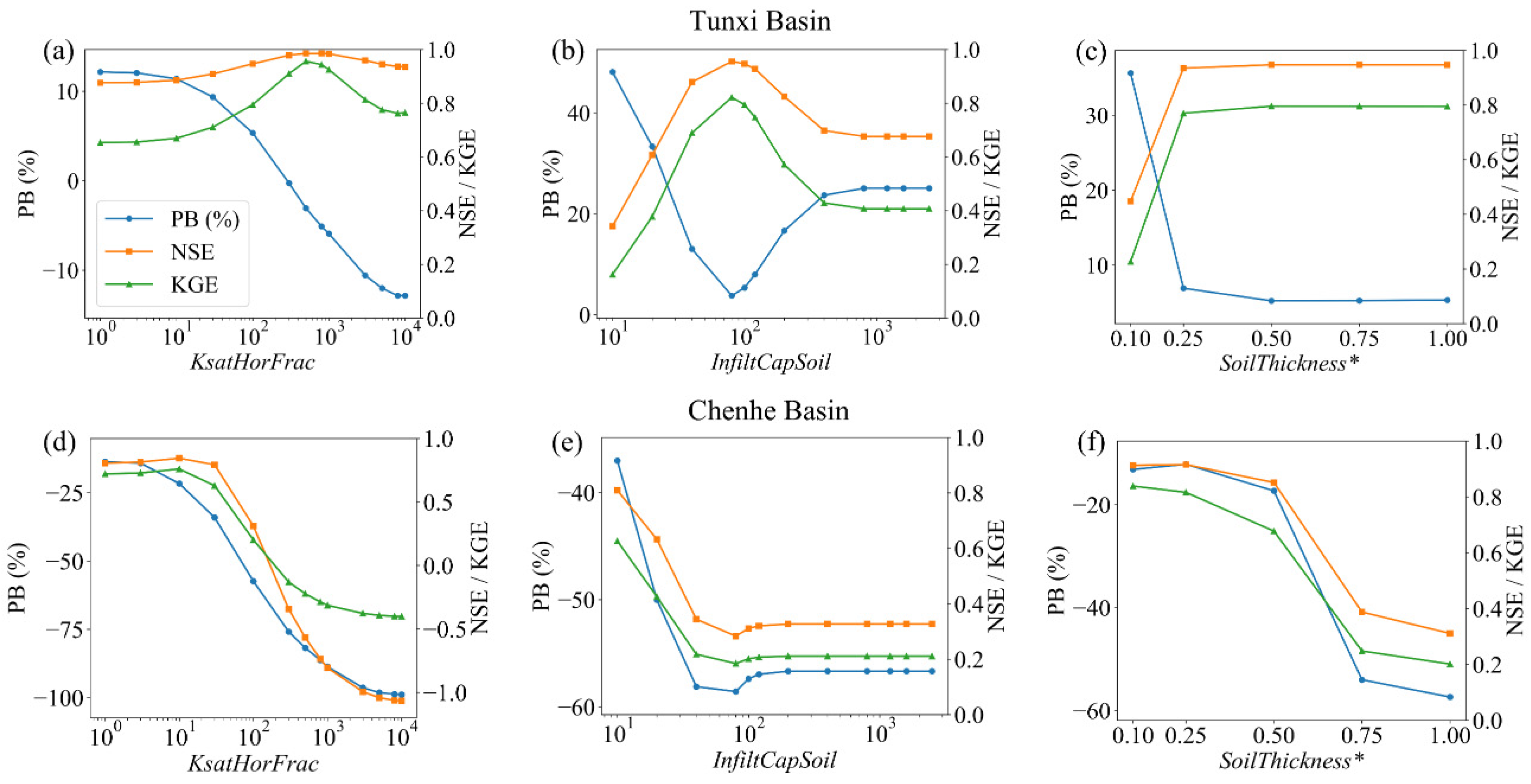
The sensitivity analysis results for three key parameters—KsatHorFrac, InfiltCapSoil, and SoilThickness—are presented in Figure 2, and the corresponding simulated hydrographs are shown in Figure 3 for the Tunxi (humid) and Chenhe (semi-humid) catchments.

4.1.1. Sensitivity Analysis

For the Tunxi catchment, the model exhibits pronounced sensitivity to KsatHorFrac, with the relative bias (PB) increasing steadily as the parameter value rises (Figure 2a). Lower KsatHorFrac values lead to a faster subsurface response and sharper flood peaks, while higher values attenuate the peak, as indicated by the hydrographs (Figure 3a,b). The InfiltCapSoil parameter shows a nonlinear response: PB first decreases and then increases, while NSE and KGE rise and then decline (Figure 2b). The model is most sensitive when InfiltCapSoil < 400 mm·day⁻¹, beyond which the hydrographs nearly overlap (Figure 3c). This indicates that infiltration capacity becomes non-limiting once rainfall can fully infiltrate, leading to diminished sensitivity. For SoilThickness, PB decreases and both NSE and KGE increase as the soil layer deepens (Figure 2c), reflecting improved storage and delayed surface runoff. Sensitivity is highest when SoilThickness is less than 0.25 times the default value, beyond which additional depth exerts little influence.

For the Chenhe catchment, PB, NSE, and KGE all decrease consistently with increasing KsatHorFrac (Figure 2d). Figure 3b also suggests that increasing KsatHorFrac reduces surface runoff and flood peaks. Unlike Tunxi, InfiltCapSoil in Chenhe shows a monotonic decline in performance metrics with increasing values (Figure 2e). Sensitivity is particularly high when InfiltCapSoil < 80 mm·day⁻¹, but stabilizes thereafter, indicating a rapid shift from infiltration-excess- to saturation-excess-dominated runoff (Figure 3d). For SoilThickness, PB, NSE, and KGE all decline with increasing depth (Figure 2f), and sensitivity remains high across the range tested. Thicker soils substantially increase storage, enhance subsurface contributions, and attenuate surface runoff response (Figure 3e,f).

Overall, KsatHorFrac and InfiltCapSoil exert the greatest control on model behavior in the humid Tunxi catchment, while KsatHorFrac and SoilThickness dominate in the semi-humid Chenhe catchment. These contrasting sensitivities highlight fundamental differences in runoff generation mechanisms under distinct hydroclimatic and soil conditions.

4.1.2. Model Calibration and Validation

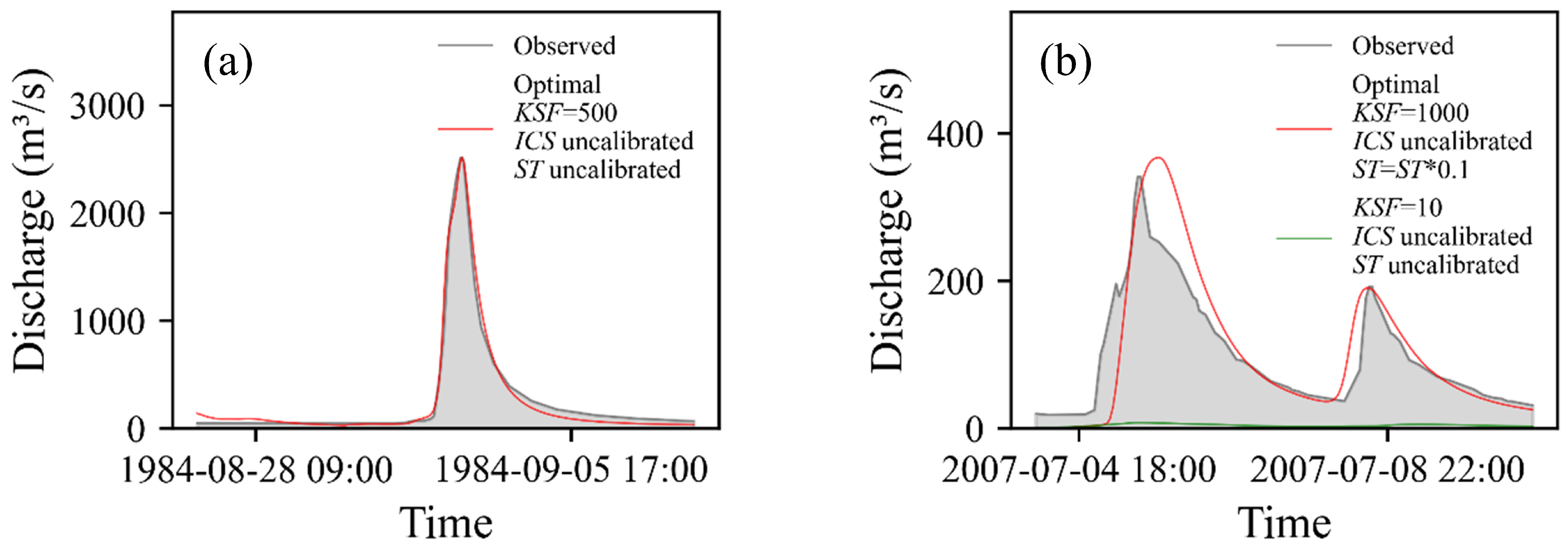
Based on the sensitivity results, parameter calibration was performed for both catchments to optimize flood simulation performance. In the Tunxi catchment, satisfactory flood reproduction was achieved by increasing KsatHorFrac to 500 while retaining the default values for InfiltCapSoil (100 mm·day⁻¹) and SoilThickness (Figure 4a). In the Chenhe catchment, however, increasing KsatHorFrac alone caused severe underestimation of flood peaks, with almost no runoff response. Reducing InfiltCapSoil provided little improvement. The most effective configuration was obtained when KsatHorFrac was increased to 1000 and SoilThickness was reduced to 10% of its original value, which significantly improved both peak discharge and total runoff volume simulation (Figure 4b). The result suggests that SoilThickness plays a dominant role in controlling flood volume and peak discharge in semi-humid mountainous catchments.

4.2. Performance of Both wflow_sbm and XAJ Models in Humid and Semi-Humid Regions

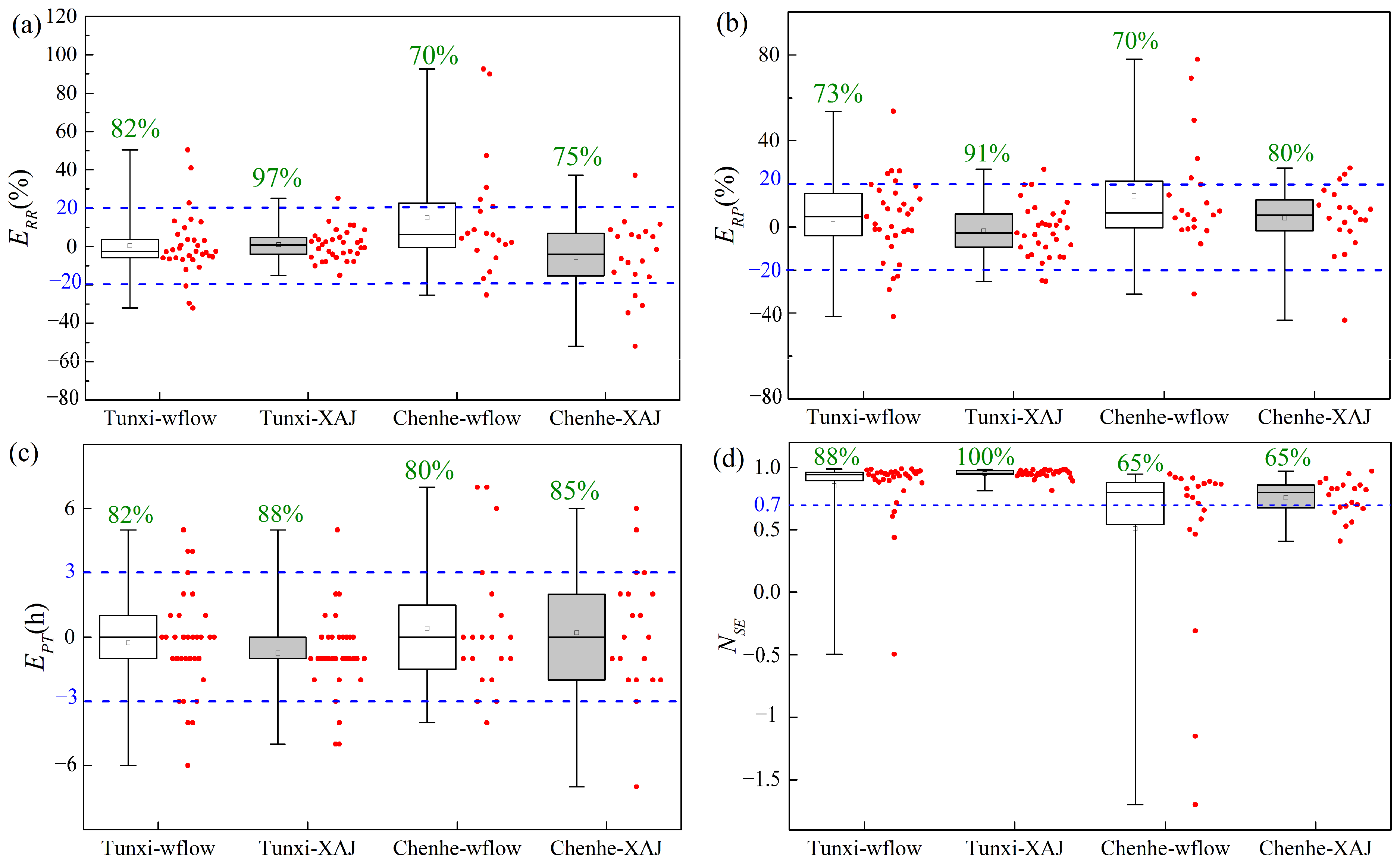
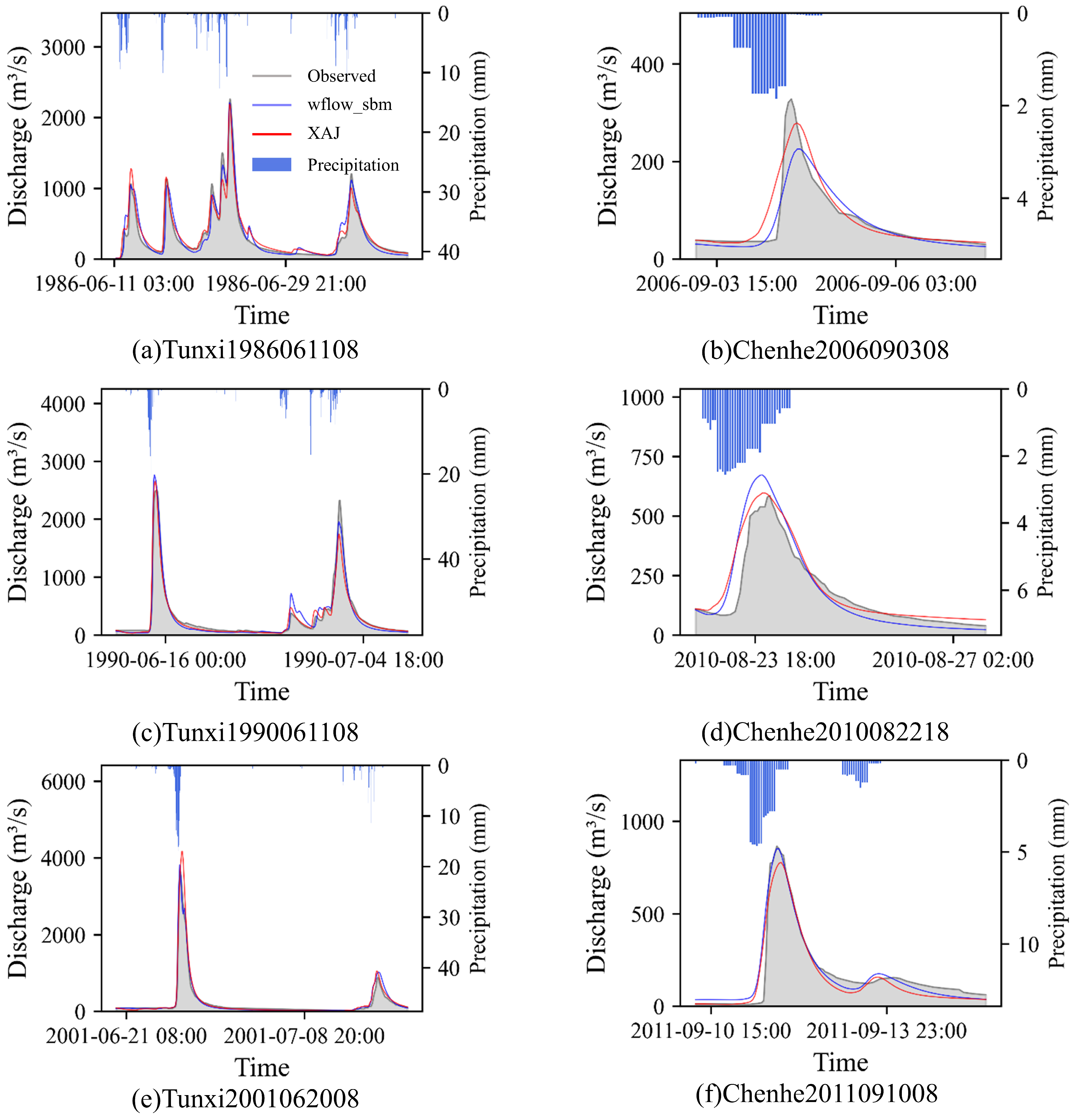
Figure 5 shows the statistical distributions of the relative volume error (E_RR), relative peak error (E_RP), peak timing error (E_PT), and Nash–Sutcliffe efficiency coefficient (N_SE) for both the wflow_sbm and XAJ models in the Tunxi and Chenhe catchments. Representative simulated and observed flood hydrographs are shown in Figure 6. Overall, both models reproduce flood processes reasonably well in the two catchments, though the XAJ model consistently performs slightly better than wflow_sbm. Model performance is generally higher in the humid Tunxi catchment than in the semi-humid Chenhe catchment.

In the humid Tunxi catchment (Figure 5a–d), the wflow_sbm model achieves strong simulation skill, with qualified rates of 82%, 73%, and 82% for E_RR, E_RP, and E_PT, respectively, and an average N_SE of 0.85. The NSE further reaches 0.93 during the validation period, as detailed in

Table 4. Characteristic statistics of simulations by wflow_sbm model for catchments Tunxi and Chenhe.

Catchments	Model	Period	Qualified Ratio (%)			Absolute Mean			Average
			RRE	RPE	PTE	RRE (%)	RPE (%)	PTE (h)	NSE
Tunxi	wflow	Calibration	72	68	77	13.6	15.3	1.6	0.82
		Validation	100	82	93	5.8	12.4	1.8	0.93
	XAJ	Calibration	100	86	86	6.2	10.6	1.3	0.95
		Validation	91	100	91	6.1	8.0	1.6	0.95
Chenhe	wflow	Calibration	62	69	69	20.7	19.3	2.8	0.49
		Validation	71	71	100	22.3	17.5	1.1	0.54
	XAJ	Calibration	77	77	77	14.6	13.1	2.5	0.74
		Validation	71	86	100	19.0	10.3	1.9	0.80

. The XAJ model performs slightly better, achieving qualified rates of 97% (E_RR), 91% (E_RP), and 88% (E_PT), and a mean N_SE of 0.95. Table 4 shows that its NSE remains stable at 0.95 during both calibration and validation periods. Both models capture flood peaks and recession limbs in close agreement with the observed hydrographs (Figure 6a,c,e). In the semi-humid Chenhe catchment(Figure 5a–d), the overall model performance is poorer than that in Tunxi catchment. The wflow_sbm model achieves qualified rates of 70%, 70%, and 80% for E_RR, E_RP, and E_PT, respectively, with a mean N_SE of 0.51, whereas the XAJ model yields slightly higher values (75%, 80%, and 85%) and a mean N_SE of 0.76. Further analysis of the temporal statistics (Table 4) reveals that in the Chenhe catchment, wflow_sbm attains an NSE of only 0.49 during calibration, which improves to 0.54 in validation, still notably lower than the XAJ model (0.74 in calibration and 0.80 in validation).

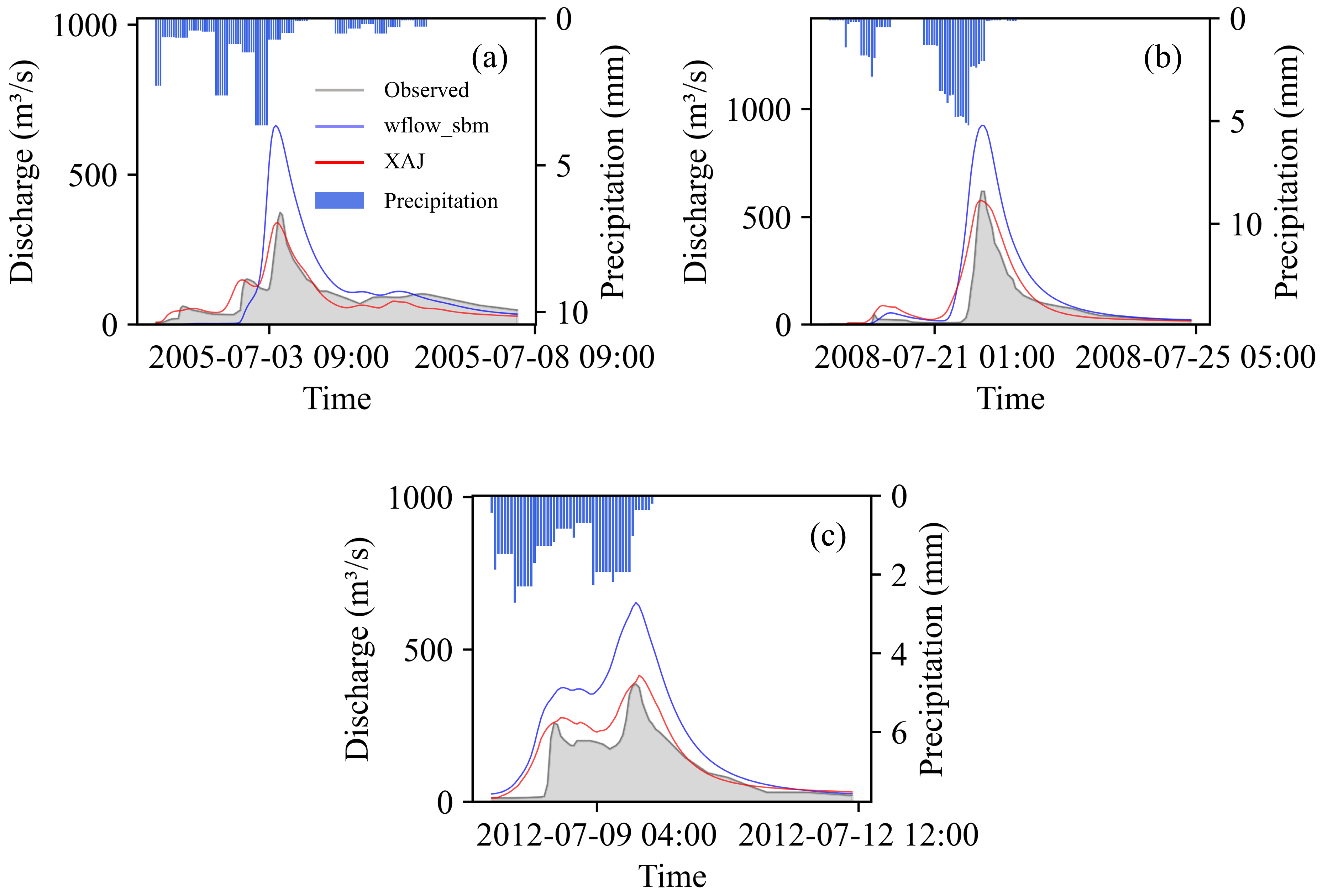
In addition, according to the boxplot results, three flood events in the Chenhe catchment exhibit N_SE values below zero, indicating poor simulation performance. These three storm events show notably larger deviations between observed and simulated discharges (Figure 7). In these cases, the wflow_sbm model tends to overestimate both total runoff and peak discharge, whereas simulated peaks of the XAJ model are closer to the observations. Even so, for the other flood events, as illustrated in Figure 6b,d,f, both wflow_sbm and XAJ exhibit comparable performance, showing a close agreement with the observed hydrographs in terms of peak timing and recession behavior.

4.3. Internal Sub-Catchment Simulation Results

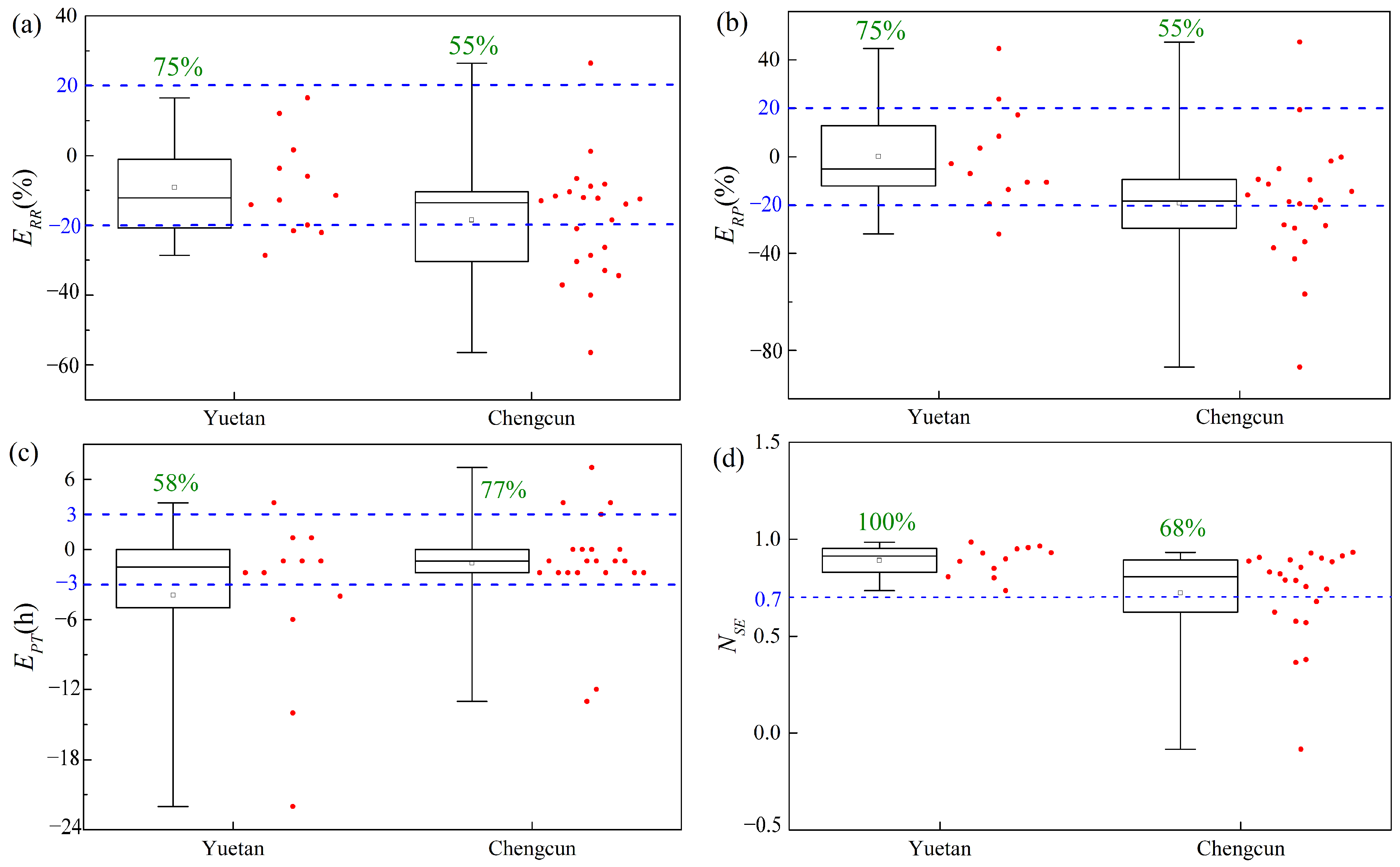
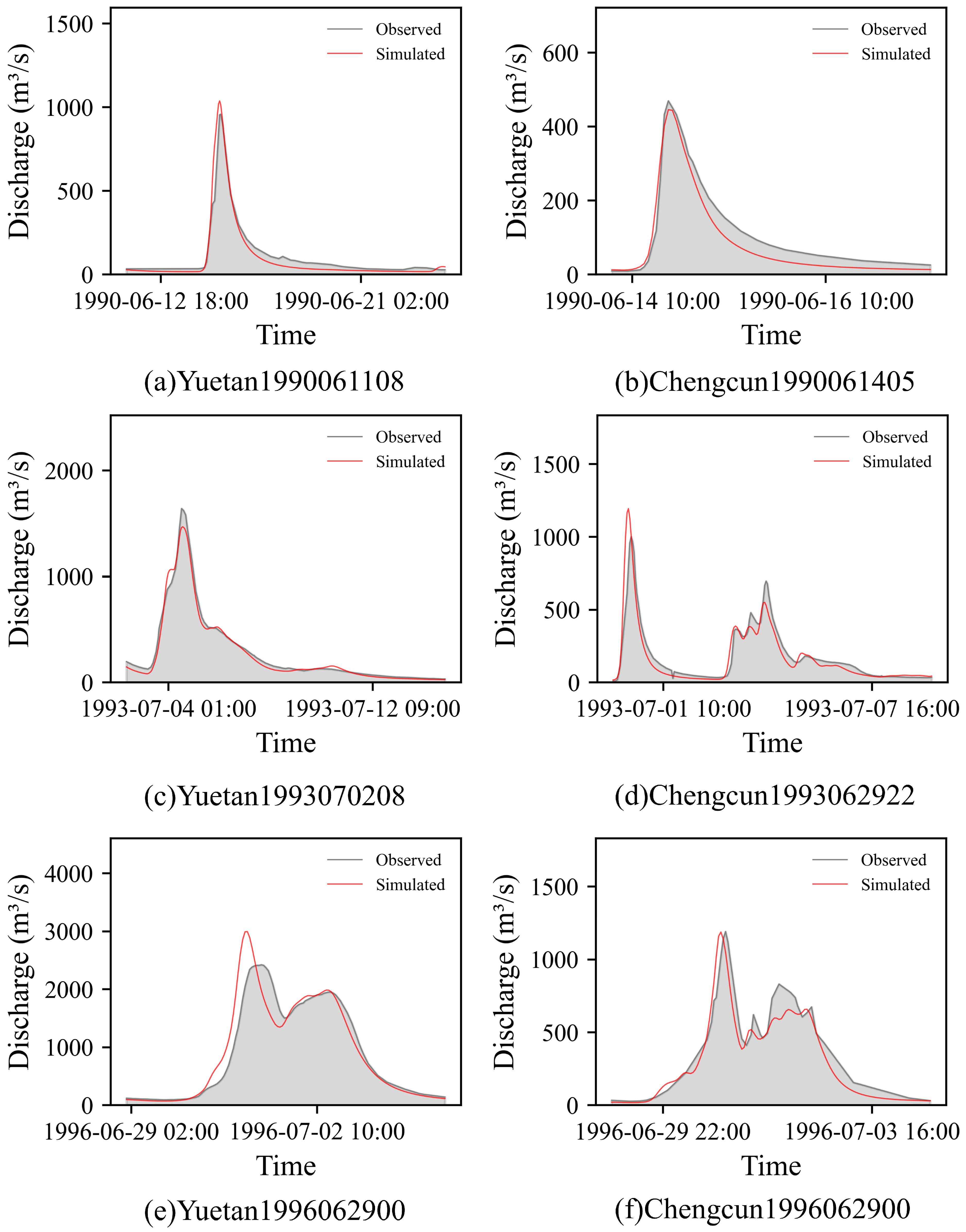
Figure 8 presents the statistical evaluation of flood simulations at two interior sub-catchments—Yuetan and Chengcun—within the Tunxi catchment. The Yuetan sub-catchment demonstrates consistently better performance across all metrics, with the distributions of E_RR, E_PR, E_PT, and N_SE showing tighter clustering around the ideal values. Median E_RR and E_PR are both close to zero (Figure 8a,b), and the proportions of qualified events reach 75%. The qualified rate of E_PT is 58% (Figure 8c) and all N_SE values exceed 0.7 (qualified rate 100%, Figure 8d), suggesting that the simulated hydrographs reproduce the timing and magnitude of observed flows well. In contrast, the Chengcun sub-catchment exhibits moderately lower accuracy, with qualified rates of 55% for E_RR and E_PR, 77% for E_PT, and 68% for N_SE. Flood peaks are generally reproduced with slight underestimation, but the overall hydrograph shape remains consistent with observations. Figure 9 further illustrates that the model accurately captures multi-peak flood responses in the Yuetan sub-catchment (Figure 9a,d,e), with peak discharge deviations within 10% and realistic recession behavior. For the Chengcun sub-catchment (Figure 9b,d,f), simulated peaks occur approximately 3 h earlier and are overestimated by around 15% in the 1993062922 event, suggesting that the local flow routing representation could be further improved in steep, highly variable terrain.

Overall, the wflow_sbm model also performs well at the interior gauging stations. Both Yuetan and Chengcun show good agreement between simulated and observed hydrographs, with satisfactory reproduction of flood peaks, peak timing, and recession behavior. These results indicate that the model can maintain consistent performance not only at the basin outlet but also within the internal drainage network, confirming its reliability in representing spatially distributed hydrological responses across the catchment.

5. Discussion

This study highlights the contrasting hydrological responses and model behaviors between humid and semi-humid catchments when applying the distributed wflow_sbm and semi-distributed XAJ models. The discussion below integrates the key findings regarding parameter sensitivity and interactions, regional model performance, and sources of simulation errors.

5.1. Comparing Parameter Sensitivity in Humid and Semi-Humid Catchments

Sensitivity analysis revealed distinct dominant parameters between the two basins. In the humid Tunxi basin, KsatHorFrac and InfiltCapSoil were the most sensitive, whereas in the semi-humid Chenhe basin, KsatHorFrac and SoilThickness exerted the strongest influence. The high sensitivity of KsatHorFrac in both basins aligns with previous wflow_sbm applications [18,51,52,53] and is consistent with findings from other distributed models (e.g., VIC, WRF-Hydro) [54,55], where parameters controlling vertical/subsurface flow velocity are often key determinants of flood peak simulation.

The contrasting sensitivity of InfiltCapSoil between the two catchments can be attributed to differences in rainfall regimes and the associated runoff generation processes. In the humid Tunxi catchment, storm events are typically of high intensity and short duration, frequently exceeding the infiltration capacity. Under these conditions, InfiltCapSoil directly governs the partitioning between infiltration and infiltration-excess runoff, such that changes in this parameter substantially modify both flood peak magnitude and hydrograph shape. In the semi-humid Chenhe catchment, however, rainfall intensities are generally lower and more spatially variable. Within the parameter range tested in this study, rainfall seldom approaches the infiltration capacity, meaning that the system rarely transitions into an infiltration-excess dominated regime. Instead, runoff formation is primarily controlled by soil saturation dynamics and subsurface flow processes. Therefore, variations in InfiltCapSoil exert only a limited influence on flood response, resulting in the much weaker parameter sensitivity observed in Chenhe.

Similarly, the sensitivity of SoilThickness differs markedly between the two basins owing to contrasting soil and moisture conditions. In the humid Tunxi catchment, soils are generally deeper and maintain relatively high antecedent moisture. Under these circumstances, the default SoilThickness (~2 m) already provides sufficient storage to represent subsurface retention and delayed flow pathways, such that further adjustments to the soil depth have only a limited influence on runoff generation. In contrast, the Chenhe catchment is characterized by shallower soils and a much thinner unsaturated zone, which constrains effective storage capacity. In this setting, even small changes in SoilThickness substantially affect the balance between infiltration and runoff, modify antecedent wetness conditions, and shift the relative contribution of saturation-excess and infiltration-excess runoff processes. This explains why SoilThickness becomes a primary control on flood peaks in the semi-humid basin. Similar basin-dependent sensitivities of soil depth have also been reported in previous distributed modeling studies, including VIC applications across Chinese catchments [55].

Overall, these results indicate that the sensitivity of key parameters such as InfiltCapSoil and SoilThickness is strongly basin-dependent and governed by local hydro-geomorphic characteristics, particularly soil depth, storage capacity, and rainfall intensity regime. This highlights the need to account for catchment-specific conditions when calibrating DHMs and when transferring parameters across regions.

A key limitation of this sensitivity analysis is its focus on only three parameters (KsatHorFrac, InfiltCapSoil, SoilThickness). These were selected because they directly control the dominant runoff generation processes in wflow_sbm. This focused approach allowed us to efficiently explore process-based contrasts between hydroclimatic regimes. However, the wflow_sbm model contains a broader parameter space (over 25 tunable parameters). Parameters governing evapotranspiration, river routing, or other subsurface processes may also influence model outcomes, particularly under different event conditions or in catchments with distinct characteristics. Future research should therefore expand the sensitivity analysis to include a more comprehensive set of parameters to gain a fuller understanding of model behavior.

5.2. Parameter Interactions Between wflow_sbm Model and XAJ Model

Further calibration revealed a key difference in soil thickness requirements between the two basins. In the humid Tunxi basin, the default SoilThickness produced reasonable results and required no major adjustment. In contrast, for the semi-humid Chenhe basin, the SoilThickness had to be reduced to about 10% of its default value to avoid severe underestimation of both flood volume and peak discharge. This confirms the high sensitivity of this parameter in Chenhe, consistent with the results of the sensitivity analysis. The optimized subsurface thickness in Chenhe was only about 0.2 m. This value aligns well with the basin’s observed hydrogeological conditions: steep slopes, shallow soils, and near-surface bedrock. Here, rainfall infiltration and runoff generation are largely confined to the upper soil layer. The dominant runoff mechanisms are a mix of saturation-excess and infiltration-excess flow, which involve a much thinner “active” hydrological layer than in deep-soil humid basins. Using this shallow layer in the model allows rainfall to be efficiently converted into overland flow and interflow, producing flood peaks and timing that match observations. Conversely, the default 2 m depth creates excessive soil storage, delays runoff, and attenuates flood peaks. Therefore, the calibrated 0.2 m likely represents the true effective hydrological depth of the Chenhe basin.

Furthermore, the adjusted SoilThickness in wflow_sbm shows a reasonable correspondence with the vadose zone thickness inferred from the XAJ model. Similarly to the wflow_sbm model, the soil column is conceptualized as a layer with finite thickness. Accordingly, the tension water capacity $WM(i,j)$ for each grid cell in XAJ model can be estimated using the classical definition of available soil water capacity (Equation (13)).

$$WM=({\theta }_{fc}-{\theta }_{wp})L_a$$

(13)

where ${\theta }_{fc}$ and ${\theta }_{wp}$ are the field capacity and wilting point, respectively, and $L_a$ is the vadose zone depth (mm). Using the maximum and minimum $WM$ values, the range of $L_a$ can be inferred. The maximum tension water capacity $W_{max}$ is given by

$$W_{max}=(1+B)WM$$

(14)

where $B=0.3$ and $WM=180\mathrm{mm}$, yielding $W_{max}=234\mathrm{mm}$. Assuming ${\theta }_{fc}=0.3$ and ${\theta }_{wp}=0.1$, the corresponding maximum $L_a$ is 1.17 m. According to variable contribution area theory, the unsaturated zone tends to be thin near channels and thicker on hillslopes. Thus, we assume $L_a\approx 0$ near saturated channel cells. Overall, the inferred unsaturated zone depth in the basin ranges from 0 to 1.17 m, with an average of approximately 0.55 m. After applying the SoilThickness adjustment, the effective subsurface layer thickness in wflow_sbm is approximately 0.2 m, which is close to this average value. This consistency suggests that the adjusted subsurface thickness is physically reasonable and highlights the necessity of modifying this parameter in semi-humid basins such as Chenhe.

5.3. Regional Model Performance and Implications

Both the distributed wflow_sbm and the semi-distributed XAJ model demonstrated satisfactory performance in the humid Tunxi catchment. The robust performance of wflow_sbm at internal stations (N_SE > 0.7) confirms that its spatially distributed parameters, derived from seamless global datasets, are generally reliable for humid environments. In the semi-humid Chenhe basin, wflow_sbm achieved overall acceptable accuracy, simulating most flood events comparably to the XAJ model. However, it substantially overestimated runoff volume and peak discharge in three events, highlighting a key challenge in semi-humid applications.

The observed overestimation appears to be the most plausible reason for inaccuracies in representing antecedent soil moisture within wflow_sbm. Operating in continuous simulation mode, wflow_sbm relies on globally available, coarse-resolution meteorological forcing. Persistent minor biases in precipitation or evapotranspiration within these datasets can accumulate, leading to systematic errors in simulated soil water storage prior to rainfall events. In contrast, the XAJ model benefits from its unique two-stage structure: a daily soil moisture accounting module provides a stabilized and often more accurate estimate of antecedent soil moisture, which is then used to initialize the hourly flood routing module. This structural advantage allows the XAJ model to better capture antecedent wetness conditions, resulting in more reliable flood simulations, particularly for event-based modeling.

These findings have clear practical implications. The wflow_sbm model, with its spatially explicit framework, is a valuable tool for flood simulation in small- to medium-sized humid and semi-humid catchments, especially under data-scarce conditions where its parameterization approach is advantageous. However, its application in semi-humid regions requires careful attention to key parameters like SoilThickness, for which calibration ranges can be informed by established models like the XAJ. When sufficient local data is available, the XAJ model is still an efficient and reliable option because of its simple structure and proven performance. These findings offer a methodological foundation for shifting flood management away from reliance on localized station data and towards a more detailed, physics-based approach that accounts for spatial differences, particularly enhancing flood risk management capabilities in small- and medium-sized basins.

To enhance the reliability of distributed models like wflow_sbm in transitional climate zones, future efforts should prioritize improving the accuracy of antecedent condition simulation. This can be achieved by (1) assimilating in situ or remotely sensed soil moisture data to correct model states, and (2) utilizing higher-resolution, bias-corrected meteorological forcing to reduce input-driven errors. Furthermore, to better understand parameter behavior, future work should extend the sensitivity analysis to a broader set of flood events with varying characteristics (e.g., intensity, duration, antecedent conditions) to obtain more generalizable insights into parameter controls. A promising way forward is to combine the strengths of both model types. This means integrating the effective soil moisture handling of conceptual models like XAJ with the spatial detail of distributed models.

6. Conclusions

To improve the accuracy of flood discharge simulation in small- and medium-sized catchments, this study selected the Tunxi catchment in a humid region and the Chenhe catchment in a semi-humid region of China as representative study areas. The conceptual distributed wflow_sbm model was used to analyze the sensitivity of runoff parameters in the two catchments. Based on this, the seamless parameter maps provided by the model preprocessing software HydroMT were further adjusted, and the simulation results were compared with those of the semi-distributed XAJ model, which has been widely applied in humid and semi-humid regions of China. The conclusions are summarized as followed:

(1)

In the humid Tunxi basin, KsatHorFrac and InfiltCapSoil were the most sensitive parameters, whereas in the semi-humid Chenhe basin, KsatHorFrac and SoilThickness showed markedly higher influence. These results highlight that the sensitive parameters of wflow_sbm differ between humid and semi-humid catchments, reflecting distinct hydrological controls in the two climatic regimes.

(2)

Using the default HydroMT SoilThickness (~2 m) in Chenhe resulted in underestimated runoff volume and peak discharge for several events. By uniformly scaling down the wflow_sbm subsurface layer (yielding a maximum soil depth of 0.2 m), the adjusted soil profile aligned closely with the vadose-zone thickness inferred from the XAJ model. This consistency confirms that SoilThickness is a key control in semi-humid catchments and underscores the necessity and physical rationality of adjusting subsurface depth when applying wflow_sbm in a semi-humid region.

(3)

In both the Tunxi and Chenhe basins, the wflow_sbm model demonstrated comparable performance to the XAJ model, indicating its strong applicability in both humid and semi-humid catchments and confirming the effectiveness of the adopted seamless parameter estimation maps. Specifically, in the humid Tunxi catchment, wflow_sbm achieved a mean N_SE of 0.85, with N_SE values exceeding 0.7 at both internal stations. In the semi-humid Chenhe basin, the model successfully reproduced most flood events, with N_SE values generally above 0.7, performing similarly to the XAJ model. However, three flood events showed noticeable overestimation in both flood volume and peak discharge. This discrepancy may be attributed to inaccuracies in simulating antecedent soil moisture conditions in the model. Therefore, future research should focus on incorporating soil moisture data assimilation and using higher-resolution land-surface datasets to improve the representation of initial conditions and enhance simulation accuracy.

(4)

Overall, the wflow_sbm model is applicable for flood forecasting in small- and medium-sized catchments in humid and semi-humid regions, and it is particularly advantageous under data-scarce basins. However, its application in semi-humid basins requires the adjustment of SoilThickness, which can be guided by parameter ranges inferred from the XAJ model for such regions.

References

1. Zang, S.; Li, Z.; Zhang, K.; Yao, C.; Liu, Z.; Wang, J.; Huang, Y.; Wang, S. Improving the flood prediction capability of the Xin’anjiang model by formulating a new physics-based routing framework and a key routing parameter estimation method. J. Hydrol. 2021, 603, 126867. [Google Scholar] [CrossRef]
2. Wagener, T.; Wheater, H.; Gupta, H.V. Rainfall-Runoff Modelling in Gauged and Ungauged Catchments; World Scientific: Singapore, 2004. [Google Scholar]
3. Todini, E. Rainfall-runoff modeling—Past, present and future. J. Hydrol. 1988, 100, 341–352. [Google Scholar] [CrossRef]
4. Beven, K.J. Rainfall-Runoff Modelling: The Primer; John Wiley and Sons: Hoboken, NJ, USA, 2011. [Google Scholar]
5. Liu, Z.; Todini, E. Towards a comprehensive physically-based rainfall-runoff model. Hydrol. Earth Syst. Sci. 2002, 6, 859–881. [Google Scholar] [CrossRef]
6. Liang, X.; Wood, E.F.; Lettenmaier, D.P. Surface soil moisture parameterization of the VIC-2L model: Evaluation and modification. Glob. Planet. Change 1996, 13, 195–206. [Google Scholar] [CrossRef]
7. Sun, M.; Li, Z.; Yao, C.; Liu, Z.; Wang, J.; Hou, A.; Zhang, K.; Huo, W.; Liu, M. Evaluation of flood prediction capability of the WRF-hydro model based on multiple forcing scenarios. Water 2020, 12, 874. [Google Scholar] [CrossRef]
8. Van Verseveld, W.J.; Weerts, A.H.; Visser, M.; Buitink, J.; Imhoff, R.O.; Boisgontier, H.; Bouaziz, L.; Eilander, D.; Hegnauer, M.; Velden, C.T.; et al. Wflow_sbm v0.7.3, a spatially distributed hydrologic model: From global data to local applications. Geosci. Model Dev. Discuss. 2024, 17, 3199–3234. [Google Scholar] [CrossRef]
9. Yamazaki, D.; Ikeshima, D.; Sosa, J.; Bates, P.D.; Allen, G.H.; Pavelsky, T.M. MERIT Hydro: A high-resolution global hydrography map based on latest topography dataset. Water Resour. Res. 2019, 55, 5053–5073. [Google Scholar] [CrossRef]
10. Hengl, T.; Mendes de Jesus, J.; Heuvelink, G.B.; Ruiperez Gonzalez, M.; Kilibarda, M.; Blagotić, A.; Shangguan, W.; Wright, M.N.; Geng, X.; Bauer-Marschallinger, B.; et al. SoilGrids250m: Global gridded soil information based on machine learning. PLoS ONE 2017, 12, e0169748. [Google Scholar] [CrossRef]
11. Buchhorn, M.; Smets, B.; Bertels, L.; Lesiv, M.; Tsendbazar, N.-E.; Herold, M.; Fritz, S. Copernicus Global Land Service: Land Cover 100 m, Epoch 2015, Globe, Version 2.0.2 [Dataset]. 2019. Available online: https://land.copernicus.eu/global/products/lc (accessed on 30 May 2025).
12. Kowalczyk, E.; Wang, Y.; Law, R.; Davies, H.; Mcgregor, J.; Abramowitz, G. The CSIRO Atmosphere Biosphere Land Exchange (CABLE) model for use in climate models and as an offline model, CSIRO. Mar. Atmos. Res. 2006, 13, 42. [Google Scholar]
13. Van Looy, K.; Bouma, J.; Herbst, M.; Koestel, J.; Minasny, B.; Mishra, U.; Montzka, C.; Nemes, A.; Pachepsky, Y.A.; Padarian, J.; et al. Pedotransfer functions in Earth system science: Challenges and perspectives. Rev. Geophys. 2017, 55, 1199–1256. [Google Scholar] [CrossRef]
14. Koren, V.; Smith, M.; Duan, Q. Use of a priori parameter estimates in the derivation of spatially consistent parameter sets of rainfall-runoff models. Calibration Watershed Models 2003, 6, 239–254. [Google Scholar]
15. Samaniego, L.; Kumar, R.; Attinger, S. Multiscale parameter regionalization of a grid-based hydrologic model at the mesoscale. Water Resour. Res. 2010, 46, W05523. [Google Scholar] [CrossRef]
16. Rakovec, O.; Kumar, R.; Attinger, S.; Samaniego, L. Improving the realism of hydrologic model functioning through multivariate parameter estimation. Water Resour. Res. 2016, 52, 7779–7792. [Google Scholar] [CrossRef]
17. Vertessy, R.A.; Elsenbeer, H. Distributed modeling of storm flow generation in an Amazonian rain forest catchment: Effects of model parameterization. Water Resour. Res. 1999, 35, 2173–2187. [Google Scholar] [CrossRef]
18. Imhoff, R.; van Verseveld, W.; van Osnabrugge, B.; Weerts, A. Scaling point-scale (pedo) transfer functions to seamless large-domain parameter estimates for high-resolution distributed hydrologic modeling: An example for the Rhine River. Water Resour. Res. 2020, 56, e2019WR026807. [Google Scholar] [CrossRef]
19. Eilander, D.; Boisgontier, H.; Bouaziz, L.J.E.; Buitink, J.; Couasnon, A.; Dalmijn, B.; Hegnauer, M.; de Jong, T.; Loos, S.; Marth, I.; et al. HydroMT: Automated and reproducible model building and analysis. J. Open Source Softw. 2023, 8, 4897. [Google Scholar] [CrossRef]
20. Liu, Y.; Luo, Y.; Li, Z.; Liu, Z.; Wang, C.; Fu, X.; Zhang, X. Spatiotemporal dynamic runoff generation process and distribution characteristics of the saturation-excess and infiltration-excess modes in the semi-humid and semi-arid regions. J. Hydrol. Reg. Stud. 2025, 61, 102589. [Google Scholar] [CrossRef]
21. Hao, G.; Li, J.; Song, L.; Li, H.; Li, Z. Comparison between the TOPMODEL and the Xin’anjiang model and their application to rainfall runoff simulation in semi-humid regions. Environ. Earth Sci. 2018, 77, 279. [Google Scholar] [CrossRef]
22. Tian, Y.; Xu, Y.; Zhang, X. Assessment of climate change impacts on river high flows through comparative use of GR4J, HBV and Xinanjiang models. Water Resour. Manag. 2013, 27, 2871–2888. [Google Scholar] [CrossRef]
23. Yao, C.; Zhang, K.; Yu, Z.; Li, Z.; Li, Q. Improving the flood prediction capability of the Xinanjiang model in ungauged nested catchments by coupling it with the geomorphologic instantaneous unit hydrograph. J. Hydrol. 2014, 517, 1035–1048. [Google Scholar] [CrossRef]
24. Yamazaki, D.; Ikeshima, D.; Tawatari, R.; Yamaguchi, T.; O’Loughlin, F.; Neal, J.C.; Sampson, C.C.; Kanae, S.; Bates, P.D. A high-accuracy map of global terrain elevations. Geophys. Res. Lett. 2017, 44, 5844–5853. [Google Scholar] [CrossRef]
25. Ghazvinian, H.; Karami, H. Evaluating the impact of meteorological parameters on road accidents using spatial analysis: A case study of Semnan province, Iran. Spat. Inf. Res. 2025, 33, 46. [Google Scholar] [CrossRef]
26. De Bruin, H.D.; Trigo, I.; Bosveld, F.; Meirink, J. A thermodynamically based model for actual evapotranspiration of an extensive grass field close to FAO reference, suitable for remote sensing application. J. Hydrometeorol. 2016, 17, 1373–1382. [Google Scholar] [CrossRef]
27. Lindström, G.; Johansson, B.; Persson, M.; Gardelin, M.; Bergström, S. Development and test of the distributed HBV-96 hydrological model. J. Hydrol. 1997, 201, 272–288. [Google Scholar] [CrossRef]
28. Rutter, A.; Morton, A.; Robins, P. A predictive model of rainfall interception in forests. II. Generalization of the model and comparison with observations in some coniferous and hardwood stands. J. Appl. Ecol. 1975, 12, 367–380. [Google Scholar] [CrossRef]
29. Gash, J. An analytical model of rainfall interception by forests. Q. J. R. Meteorol. Soc. 1979, 105, 43–55. [Google Scholar] [CrossRef]
30. Brooks, R.; Corey, A. Hydraulic Properties of Porous Media. Ph.D. Thesis, Colorado State University, Fort Collins, CO, USA, 1964. [Google Scholar]
31. Beven, K.J.; Kirkby, M.J. A physically based, variable contributing area model of basin hydrology. Hydrol. Sci. J. 1979, 24, 43–69. [Google Scholar] [CrossRef]
32. Chow, V.; Maidment, D.; Mays, L. Applied Hydrology; McGraw-Hill Book Company: New York, NY, USA, 1988. [Google Scholar]
33. Rawls, W.; Brakensiek, D. Estimation of Soil Water Retention and Hydraulic Properties. In Unsaturated Flow in Hydrologic Modeling: Theory and Practice; Springer: Dordrecht, The Netherlands, 1989; pp. 275–300. [Google Scholar]
34. Van Dijk, A.; Bruijnzeel, L. Modelling rainfall interception by vegetation of variable density using an adapted analytical model. Part 1. Model description. J. Hydrol. 2001, 247, 230–238. [Google Scholar] [CrossRef]
35. Brakensiek, D.; Rawls, W.; Stephenson, G. Modifying SCS Hydrologic Soil Groups and Curve Numbers for Rangeland Soils; ASAE Paper No. PNR-84203; American Society of Agricultural Engineers: St. Joseph, MI, USA, 1984. [Google Scholar]
36. Myneni, R.; Knyazikhin, Y.; Park, T. MOD15A3H MCD15A3H MODIS/Terra+Aqua Leaf Area Index/FPAR 4-day L4 Global 500m SIN Grid, Version 006 [Dataset]. NASA EOSDIS Land Processes Distributed Active Archive Center (DAAC): Sioux Falls, SD, USA, 2015. Available online: https://lpdaac.usgs.gov/products/mcd15a3hv006/ (accessed on 30 May 2025).
37. Engman, E.T. Roughness coefficients for routing surface runoff. J. Irrig. Drain. Eng. 1986, 112, 39–53. [Google Scholar] [CrossRef]
38. Kilgore, J.L. Development and Evaluation of a Gis-Based Spatially Distributed Unit Hydrograph Model. Ph.D. Thesis, Virginia Tech, Blacksburg, VA, USA, 1997. [Google Scholar]
39. Liu, Z.; Martina, M.L.; Todini, E. Flood forecasting using a fully distributed model: Application of the TOPKAPI model to the Upper Xixian Catchment. Hydrol. Earth Syst. Sci. 2005, 9, 347–364. [Google Scholar] [CrossRef]
40. Fan, J.; Mcconkey, B.; Wang, H.; Janzen, H. Root distribution by depth for temperate agricultural crops. Field Crops Res. 2016, 189, 68–74. [Google Scholar] [CrossRef]
41. Schenk, H.J.; Jackson, R.B. The global biogeography of roots. Ecol. Monogr. 2002, 72, 311–328. [Google Scholar] [CrossRef]
42. Pitman, J.I. Rainfall interception by bracken in open habitats—Relations between leaf area, canopy storage and drainage rate. J. Hydrol. 1989, 105, 317–334. [Google Scholar] [CrossRef]
43. Liu, S. Estimation of rainfall storage capacity in the canopies of cypress wetlands and slash pine uplands in North-Central Florida. J. Hydrol. 1998, 207, 32–41. [Google Scholar] [CrossRef]
44. Farr, T.G.; Rosen, P.A.; Caro, E.; Crippen, R.; Duren, R.; Hensley, S.; Kobrick, M.; Paller, M.; Rodriguez, E.; Roth, L.; et al. The Shuttle Radar Topography Mission. Rev. Geophys. 2007, 45, RG2004. [Google Scholar] [CrossRef]
45. Tóth, B.; Weynants, M.; Nemes, A.; Makó, A.; Bilas, G.; Tóth, G. New generation of hydraulic pedotransfer functions for Europe. Eur. J. Soil Sci. 2015, 66, 226–238. [Google Scholar] [CrossRef]
46. Leopold, L.B.; Maddock, T. The Hydraulic Geometry of Stream Channels and Some Physiographic Implications; US Government Printing Office: Washington, DC, USA, 1953. [Google Scholar]
47. Gupta, H.V.; Kling, H.; Yilmaz, K.K.; Martinez, G.F. Decomposition of the mean squared error and NSE performance criteria: Implications for improving hydrological modelling. J. Hydrol. 2009, 377, 80–91. [Google Scholar] [CrossRef]
48. GB/T 2482-2008; Standard for Hydrological Information and Hydrological Forecasting. Ministry of Water Resources of the People’s Republic of China: Beijing, China, 2008.
49. Zhao, R. The Xinanjiang model applied in China. J. Hydrol. 1992, 135, 371–381. [Google Scholar] [CrossRef]
50. Duan, Q.; Sorooshian, S.; Gupta, V. Effective and efficient global optimization for conceptual rainfall-runoff models. Water Resour. Res. 1992, 28, 1015–1031. [Google Scholar] [CrossRef]
51. Wannasin, C.; Brauer, C.; Uijlenhoet, R.; van Verseveld, W.; Weerts, A.H. Daily flow simulation in Thailand Part I: Testing a distributed hydrological model with seamless parameter maps based on global data. J. Hydrol. Reg. Stud. 2021, 34, 100794. [Google Scholar] [CrossRef]
52. Zang, S.; Weerts, A.; van Verseveld, W.J.; Li, Z.; Huang, P. Compound effects of river routing and local rainfall-runoff for inflow simulation of a large reservoir. Hydrol. Sci. J. 2025, 70, 1541–1553. [Google Scholar] [CrossRef]
53. Rusli, S.; Weerts, A.; Taufiq, A.; Bense, V. Estimating water balance components and their uncertainty bounds in highly groundwater-dependent and data-scarce area: An example for the Upper Citarum basin. J. Hydrol. Reg. Stud. 2021, 37, 100911. [Google Scholar] [CrossRef]
54. Liu, Y.; Liu, J.; Li, C.; Yu, F.; Wang, W.; Qiu, Q. Parameter sensitivity analysis of the WRF-hydro modeling system for streamflow simulation: A case study in semi-humid and semi-arid Catchments of Northern China. Asia-Pac. J. Atmos. Sci. 2021, 57, 451–466. [Google Scholar] [CrossRef]
55. Gou, J.; Miao, C.; Duan, Q.; Tang, Q.; Di, Z.; Liao, W.; Wu, J.; Zhou, R. Sensitivity analysis-based automatic parameter calibration of the VIC model for streamflow simulations over China. Water Resour. Res. 2020, 56, e2019WR025968. [Google Scholar] [CrossRef]
Figure 1. Elevation map of the study areas derived from the Shuttle Radar Topography Mission (SRTM) digital elevation model, and the locations of hydrological and rainfall gauge stations.
Water 18 00417 g001
Figure 2. Sensitivity analysis of key parameters in the wflow_sbm model for two representative catchments. Panels (ac) show the results for the Tunxi catchment and (df) for the Chenhe catchment. Model performance metrics PB, NSE, and KGE were used to evaluate the response to variations in KsatHorFrac, InfiltCapSoil, and SoilThickness. The symbol *denotes a multiplier relative to the baseline SoilThickness value derived from HydroMT.
Water 18 00417 g002
Figure 3. Simulated hydrographs under different parameter values for the Tunxi and Chenhe catchments. The figure illustrates the model response to changes in KsatHorFrac, InfiltCapSoil, and SoilThickness, highlighting differences in hydrograph shape and magnitude between the two catchments. The symbol * denotes a multiplier relative to the baseline SoilThickness value derived from HydroMT.
Water 18 00417 g003
Figure 4. Simulated and observed hydrographs for representative flood events in two study catchments. Panels show the comparison for (a) Tunxi and (b) Chenhe catchments under different parameter calibration schemes. The abbreviations in the legend: KSF (KsatHorFrac), ICS (InfiltCapSoil), ST (SoilThickness) The symbol * denotes a multiplier relative to the baseline SoilThickness value derived from HydroMT.
Water 18 00417 g004
Figure 5. Box plots of the (a) relative volume error (ERR), (b) relative peak error (ERP), (c) peak timing error (EPT), and (d) Nash–Sutcliffe efficiency coefficient (NSE) for floods simulated by the wflow_sbm model and XAJ model in the Tunxi and Chenhe catchments.
Water 18 00417 g005
Figure 6. Comparison of observed and simulated flood hydrographs using the wflow_sbm and XAJ models in typical events of the Tunxi and Chenhe catchments.
Water 18 00417 g006
Figure 7. Comparison of observed and simulated hydrographs for three flood events (ac) in the Chenhe catchment with NSE < 0.
Water 18 00417 g007
Figure 8. Boxplots of flood simulation performance metrics for two sub-catchments within the Tunxi catchment. Panels show (a) relative volume error ( E R R ), (b) relative peak error ( E R P ), (c) peak timing error ( E P T ), and (d) Nash–Sutcliffe efficiency coefficient ( N S E ) for floods simulated by the wflow_sbm model at the Yuetan and Chengcun sub-catchments.
Water 18 00417 g008
Figure 9. Comparison of observed and simulated hydrographs for representative flood events at Yuetan and Chengcun sub-catchments using the wflow_sbm model.
Water 18 00417 g009