Optimization of Electrical Resistivity Tomography Monitoring for Weak Electrical Response Pollutants: A Coupled Field–Sand Tank Experimental Study Taking Nitrate as an Example

Abstract

Due to the weak electrical response characteristics of groundwater nitrate contamination, traditional monitoring and remediation assessment methods are limited by low spatiotemporal resolution, high cost, and strong subjectivity. To address this issue, this study proposed an integrated technical framework combining field detection, laboratory-controlled experiments, and remediation process monitoring, aiming to explore the application potential of Electrical Resistivity Tomography (ERT) in nitrate pollution monitoring and remediation evaluation. First, ERT survey lines (L1 and L2) were deployed at a chemical-contaminated site in Luzhou, Sichuan Province, and groundwater samples were collected. Coupled with hydrochemical analysis, the feasibility of ERT for identifying nitrate plumes was verified. Second, a quantitative response model between nitrate concentration and resistivity was established through Miller box experiments, and a multi-line layout was optimized via sand tank experiments to mitigate boundary effects and improve monitoring accuracy. Finally, grouped sand tank experiments involving electroactive bacteria (EAB) and magnetite were conducted. Combined with 16S rRNA sequencing, the coupling mechanism between ERT electrical responses and biogeochemical processes was elucidated. The results showed that the low-resistivity anomaly zones identified by field ERT were accurately consistent with the high-nitrate contamination zones, and Piper diagrams confirmed that nitrate-related ions were the primary cause of the low-resistivity anomalies. The power function quantitative model established by the Miller box experiment (y = 1021.97x^−0.74, R² = 0.9589) enabled the indirect inversion of nitrate concentrations, with a small deviation between theoretical and measured values in the deep layer (16–18 m). The optimized layout of one main and three auxiliary survey lines effectively characterized the spatiotemporal migration of the contamination plume. Under high-water level conditions, the ternary system of nitrate–magnetite–EAB exhibited the strongest low-resistivity response. Microbial analysis indicated that electroactive groups (e.g., Pseudomonas and Flavobacterium) enriched in the EAB group were the core drivers of enhanced electrical conductivity. The integrated ERT monitoring technology system constructed in this study realizes the visual identification of nitrate plumes and dynamic tracking of remediation processes, providing technical support for the precise monitoring and in situ remediation of nitrate contamination in agricultural non-point sources and industrial sites.

1. Introduction

The use of hazardous environmental substances in industrial activities has led to the contamination of many important aquifers worldwide. The deterioration of groundwater quality poses threats to human health, drinking water and food supply, and biodiversity. Excessive application of nitrogen fertilizers in agricultural production, as well as the improper discharge of industrial and domestic wastewater, can result in nitrate concentrations exceeding the standard limit in groundwater [1]. This makes groundwater nitrate contamination a key focus of groundwater pollution remediation. Traditional nitrate pollution monitoring methods rely on field drilling, sampling, and laboratory analysis, which involve monitoring and analyzing nitrate content in groundwater based on water sample data from boreholes. Although traditional monitoring methods offer high accuracy, they suffer from practical limitations such as long time consumption and high cost [2]. Meanwhile, their invasive nature can cause disturbances to groundwater systems. Moreover, in situ measurement data obtained from individual wells only reflect conditions at a single point within the area, which is usually insufficient to track the migration of contamination plumes or determine concentration changes outside the vicinity of the wellhead [3,4]. Therefore, developing an effective method for rapid, low-cost, and large-scale monitoring of groundwater nitrate contamination has become an urgent problem to be solved.

ERT is a geophysical method that infers the distribution of subsurface media based on subsurface resistivity distribution. It is highly sensitive to hydrogeological parameters such as porosity, temperature, salinity, and water content. With advantages including continuous spatial information, in situ non-destructiveness, rapid measurement, low cost, real-time dynamic monitoring, and wide coverage, ERT has shown great potential in groundwater nitrate pollution monitoring and remediation processes [5]. Benson et al. conducted ERT measurements at a hydrocarbon-contaminated site in Utah and identified contaminant plumes through high-resistivity anomalies [6]. Yan et al. verified that abnormally high-resistivity zones in ERT results could well characterize organochlorine-contaminated areas by combining ERT with borehole sampling at a pesticide factory in Northeast China [7]. Rucker performed ERT measurements on the surface of waste disposal trenches at Hanford, demonstrating the advantages of apparent resistivity pseudo-sections and indicating a correlation between resistivity and nitrate [8]. Gasperikova used ERT to investigate groundwater contamination at Oak Ridge, Tennessee, and found that the effect of nitrate concentration on resistivity was most significant in the range of 100–2000 mg/L [9]. However, current applications of ERT technology in pollution monitoring were mostly concentrated on contamination types with significant electrical responses, such as heavy metals and non-soluble organic pollutants [10]. This is mainly because organic pollutants such as DNAPL (Dense Non-Aqueous Phase Liquid) and LNAPL (Light Non-Aqueous Phase Liquid) often form locally distinct high-resistivity zones in aquifers, while some metal cations can cause a decrease in resistivity, thus exhibiting good electrical identifiability [11,12]. In contrast, nitrate, the focus of this study, is a highly soluble inorganic pollutant with fast migration speed and significant diffusion with groundwater flow. At the same time, its hydrochemical characteristics are close to the background of groundwater, making it difficult to form prominent high-resistivity zones similar to DNAPL/LNAPL or low-resistivity zones formed by heavy metals. Therefore, in real field sites, identifying nitrate solely based on electrical changes is often difficult, especially in the context of agricultural non-point source pollution, where nitrate signals are easily masked by complex hydrogeochemical processes [13,14,15]. For example, Wehrer M et al. used 3D ERT to depict the migration path and distribution of nitrate in soil in an intensively cultivated farmland, but the results showed that there were still obvious deviations in estimating nitrate concentrations through ERT inversion [16]. In addition, the scale of conventional ERT profiles is limited, and the low-resistivity changes caused by nitrate are often difficult to directly identify in inversion maps, requiring interpretation through multi-profile comparison. Meanwhile, resistivity changes mainly reflect the total dissolved solids level of groundwater, rather than specific pollutant information. Therefore, interpreting ERT images based on experience is prone to problems such as strong subjectivity, high ambiguity, and high risk of misjudgment.

In theoretical explorations using small-scale laboratory sand tanks, ERT often encounters significant boundary effects due to scale limitations, which have become a key factor restricting test accuracy [17,18]. Achieving high-precision ERT testing in small-scale laboratory sand tanks has thus become a practical challenge. From existing experiments, the interference of closed boundaries in small-scale sand tanks on ERT signals is mainly reflected in three aspects. First, the high-resistivity bottom boundary (e.g., Perspex base) can reflect electric current, forming a high-resistivity shadow zone, which masks the true resistivity characteristics of key target layers (e.g., clay layers) and prevents their effective resolution [19]. Second, the three-dimensional migration of pollutants (e.g., diesel) on small scales is limited by lateral boundaries [20], while conventional 2D inversion is difficult to adapt to this process, easily generating out-of-plane artifacts (e.g., anomalies in the high-resistivity zone of the base, false high-resistivity signals below deep injection points), leading to misjudgment of migration range and concentration. Third, the sensitivity of the current field decays sharply near the boundaries, greatly compressing the effective testing area, and only data in a very small central area of the tank are reliable [21]. These problems highlight the inherent contradiction in small-scale sand tank-based ERT testing. Specifically, large-scale sand tanks are not feasible for laboratory construction, whereas the boundary constraints of small scales significantly disrupt the current field distribution and inversion accuracy of ERT. Therefore, how to overcome the boundary effects caused by small scales through method optimization, boundary design, or sensitivity correction to achieve high-precision ERT testing has become an urgent practical problem in laboratory-scale research on subsurface media and contaminant migration.

In many sites, source zone contamination undergoes natural attenuation, and contaminants migrate to form groundwater contamination plumes. With the development of in situ remediation technology, more and more treatment strategies can act directly on contamination plumes within aquifers without the need for large-scale excavation or extraction treatment [22]. However, whether remediation agents and microorganisms are successfully delivered to the target aquifer and fully contact with contaminants is one of the key factors determining remediation effectiveness [23]. Therefore, it is necessary to accurately judge the diffusion range and reaction activity of injected agents within a short time scale to timely adjust injection strategies or perform secondary injection. Although traditional sampling methods can provide local chemical information, their limited spatial coverage and obvious reaction lag make it difficult to meet the needs of rapid decision-making and dynamic tracking [24]. To address this limitation, there is an urgent need for an in situ decision-making auxiliary tool for short-cycle delivery evaluation. Based on the response mechanism of subsurface media electrical changes, ERT can realize the visualization of migration and reaction processes with continuous, rapid, and high spatial resolution by means of the conductivity changes caused by agents or microorganisms [25]. For example, Orozco used ERT to monitor the biogeochemical transformations caused by microbial stimulation after acetate injection [26]. Mao et al. successfully located potassium permanganate plumes based on ERT in sand tank experiments [27] and further combined ERT with Self-Potential technology to track the diesel degradation process promoted by sulfate [28]. Therefore, ERT has shown great practical application potential in the rapid evaluation of agent delivery and conductivity changes caused by microorganisms, the monitoring of contamination plume evolution, and the identification of in situ remediation process responses.

Taking nitrate as the target pollutant, this study aims to explore an efficient monitoring and diagnosis method based on ERT to address the weak electrical response characteristics of nitrate contamination and the limitations of traditional sampling methods in spatiotemporal resolution. First, considering the lack of research methods combining field exploration and laboratory experiments at current groundwater nitrate-contaminated sites, borehole sampling was conducted at the nitrate-contaminated site, and ERT survey lines were deployed near background boreholes and the most severely contaminated boreholes. Second, sand tank experiments were carried out by injecting field background groundwater and water from nitrate-contaminated boreholes to monitor changes in resistivity. The resistivity test results were then compared with the sand tank sampling test results to determine characteristic empirical coefficients. A quantitative response relationship between nitrate concentration and resistivity changes was established, and the electrical identification conditions of nitrate under different hydrochemical backgrounds were clarified, providing a physical basis for the interpretation of its resistivity imaging. Third, to address the problem of imaging errors caused by boundary effects commonly existing in small-scale laboratory sand tank experiments, this study proposed an optimized multi-line layout strategy to improve the imaging accuracy of ERT under limited scale conditions. Fourth, this study used ERT to monitor the transport and diffusion processes of remediation agents and microorganisms, revealed the coupling relationship between electrical changes and biogeochemical reactions, and initially constructed the corresponding relationship between remediation agents, microorganisms, and ERT signals. Finally, combining resistivity imaging and water sample detection results, a technical system that can realize the visual identification of nitrate plumes and rapid feedback of remediation effectiveness was formed, providing technical support for the monitoring and in situ management of nitrate contamination in groundwater.

2. Materials and Methods

2.1. Study Area Overview, Hydrogeological Background and Investigation Methods

The study area is located in Naxi District, Luzhou City, Sichuan Province, China, which is one of the main urban areas of Luzhou City. Preliminary borehole sampling in April showed that nitrate concentrations in groundwater monitoring wells in this region exceeded the standard. Pollution source tracking indicated that this contamination was mainly related to the leakage of pollutants from the upstream nickel-based catalyst production workshop, nitric acid storage area, and water circulation device area, as well as historical legacy issues.

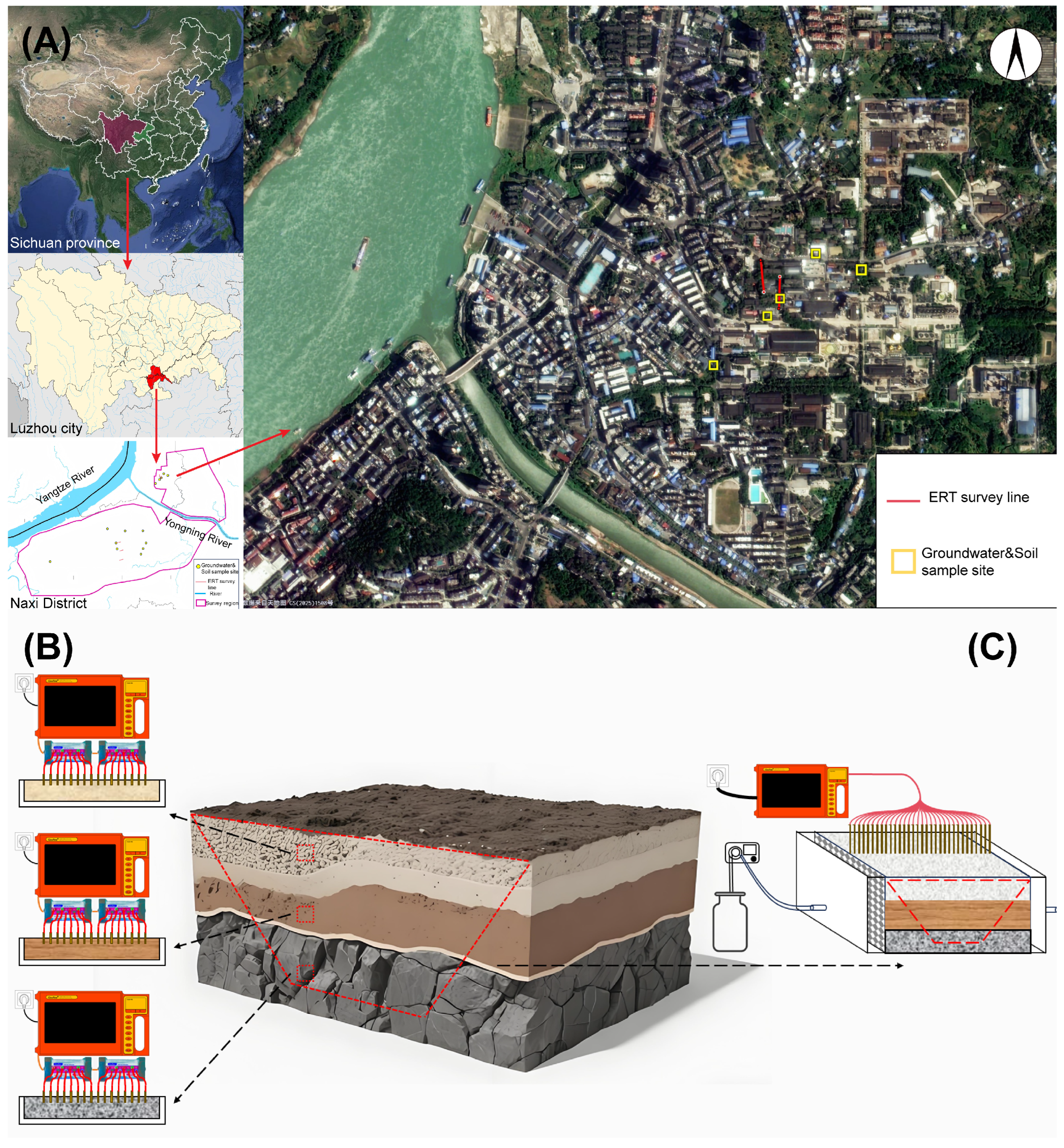
In terms of hydrogeological conditions, the study area within a depth of 0–25 m can be divided into three layers from top to bottom: the upper layer (0–8 m) is Quaternary artificial fill, mainly composed of silty clay with a small amount of gravel; the middle layer (8–20 m) is sandy gravel of the Middle Jurassic Shaximiao Formation, with argillaceous and silty structures and good water permeability, serving as the main aquifer; the lower layer (20–25 m) is sandstone of the Middle Jurassic Shaximiao Formation, with poor water permeability, forming an aquiclude. To systematically clarify the degree and spatial distribution characteristics of nitrate contamination, groundwater sampling was carried out in two phases in this study: the first phase collected water samples from 4 groundwater environmental monitoring wells in April, and 5 additional monitoring wells were sampled in June based on the detection results. Meanwhile, to reveal the spatial distribution law of the contamination plume, one 112 m (56 electrodes) and one 100 m (50 electrodes) ERT survey line were deployed near the most severely contaminated and relatively lightly contaminated monitoring wells, designated as L1 and L2, respectively (Figure 1A).

2.2. Laboratory Experimental Design

2.2.1. Miller Box Experiment

The Miller box experiment was designed to establish a quantitative response relationship between nitrate concentration and resistivity (Figure 1B), providing a calibration basis for the quantitative interpretation of field ERT monitoring results. The experiment used an acrylic box with a wall thickness of 1 cm and internal dimensions of 4 cm × 5 cm × 25 cm, filled using a wet method: an appropriate amount of ultrapure water was first added to the box, followed by the slow addition of 40–70 mesh quartz sand to ensure that the quartz sand was completely submerged in water throughout the process. The above operation was repeated until the quartz sand filling thickness reached 4 cm and a stable water film formed on the surface (the actual effective filling volume was 4 cm × 4 cm × 25 cm).

After filling, 16 copper rod electrodes were uniformly inserted into the top of the box, and the electrodes were connected to an E60DN electrical method workstation and an electrode conversion box. The experimental water was collected from the field background monitoring well (42NX), and a series of gradient nitrate solutions was prepared by adding potassium nitrate (KNO₃, purity ≥ 99.9%). Resistivity measurements were performed using the Wenner array. Due to the 16 electrodes, a maximum of 5 measurement layers could be divided. The measured apparent resistivity data were inverted using the least-squares method with the Swedish Res2dinv software (v.3.59). Considering the small size of the Miller box, deep-layer measurements were significantly affected by boundary effects, resulting in large inversion errors. Therefore, only the average value of the inverted resistivity data of the first layer was selected as the characteristic resistivity value corresponding to the nitrate concentration. The experimental concentration gradient was set according to the minimum and maximum nitrate concentrations measured in the field. By measuring the apparent resistivity at different concentrations, the nitrate concentration-resistivity response curve was finally fitted.

Given the characteristics of the Miller box, including its small size, absence of detection depth and inability for stratified packing, the results measured in this experiment correspond to the resistivity of a single point within the formation at the actual site, which constitutes a comprehensive reflection of the lithological, hydrochemical and other relevant characteristics at that point. Although the data obtained from such small-scale experiments on homogeneous media are more accurate, sandbox experiments are required to determine the overall resistivity distribution of two-dimensional profiles, thereby observing the heterogeneous resistivity distribution induced by formation inhomogeneity. Meanwhile, such experiments can also characterize the dynamic variations in low or high resistivity zones during the diffusion and migration of aqueous-phase contaminants with high or low electrical conductivity in sandy soils. This study exclusively focuses on the migration of nitrate in aquifers with groundwater flow, and thus, the sandbox was homogenously packed without stratification to minimize experimental errors.

2.2.2. Sand Tank Experiment

A three-dimensional sand tank apparatus was used to simulate the migration process of nitrate in the groundwater environment and the nitrate removal effect of the microorganism-magnetite system. The external dimensions of the sand tank were 52 cm (length) × 42 cm (width) × 21 cm (height), and the interior was divided into three parts by partitions: a water inlet chamber, a main chamber, and a water outlet chamber. The main chamber was the core simulation area with internal dimensions of 40 cm (length) × 40 cm (width) × 20 cm (height). Both the water inlet chamber and the water outlet chamber had dimensions of 4 cm (length) × 40 cm (width) × 20 cm (height) (Figure 1C). The water inlet pipe of the water inlet chamber was connected to a peristaltic pump, and the inlet flow rate was controlled by adjusting the rotational speed of the peristaltic pump. The water outlet flow rate was monitored in real-time at the water outlet pipe of the water outlet chamber using a graduated cylinder and a stopwatch. By regulating the water levels in the water inlet and outlet chambers, simulation experiments under both saturated and unsaturated aquifer conditions could be carried out, respectively. A high-density electrical main survey line (L1) with an electrode spacing of 1 cm and 32 electrodes was deployed on the top of the sand tank along the water flow direction (water inlet chamber to water outlet chamber) to monitor the dynamic changes in resistivity during contaminant migration.

(1)

Sand Tank Experiment for Monitoring Contaminant Migration

To accurately capture the spatial migration process of nitrate, in addition to the main survey line L1 on the top of the sand tank, three additional high-density electrical survey lines (L2, L3, L4) with an electrode spacing of 1 cm and 32 electrodes were deployed every 10 cm perpendicular to the water flow direction. Meanwhile, four water sampling points (A, B, C, D) were set every 8 cm along the main survey line L1, and the water sample from the outlet was designated as point E. Before the experiment, 44NX background well water was injected to saturate the sand tank, followed by the injection of 01NX high-concentration nitrate-contaminated well water. ERT detection and simultaneous collection of water samples from each sampling point were carried out at 10 min, 30 min, 1.5 h, 2.5 h, 5 h, 8 h, 12 h, 24 h, and 36 h, respectively. The experiment was terminated when the electrical conductivity at the water outlet stabilized. By comparing the ERT inversion profiles at different time points with the measured nitrate concentrations of water samples, the dynamic migration law of nitrate was revealed.

(2)

Microbial Experiment

Soil sample spheres were placed in the middle of the main chamber of the sand tank. The soil samples were collected from the chemical site in the study area. After grinding and sieving, 49 g of soil was taken to make spherical soil samples with a diameter of approximately 4 cm. The burial depth was about 2 cm below the upper surface of the quartz sand, and the surrounding area was backfilled and covered with quartz sand. A total of eight groups of soil samples were prepared. One or more distinct samples were added to each soil sample group. The added samples include: 5 mL of groundwater sample from Well 42NX (background well), 5 mL of groundwater sample from Well 01NX (high-concentration nitrate-contaminated well), 0.98 g of magnetite, 10 mL of electroactive bacterial suspension with an OD₆₀₀ of 0.8. The combination methods of adding samples to the spherical soil samples are shown in

Table 1. The sample added to each group of soil samples.

Number of Samples	The Source of the Added Water Sample (mL)	Magnetite (g)	EAB (mL)	Drying Method
1	042NX, 5	0	0	air-dried naturally
2	01NX, 5	0	0	air-dried naturally
3	042NX, 5	0.98	0	air-dried naturally
4	042NX, 5	0	10	air-dried naturally
5	01NX, 5	0.98	0	air-dried naturally
6	01NX, 5	0	10	air-dried naturally
7	042NX, 5	0.98	10	air-dried naturally
8	01NX, 5	0.98	10	air-dried naturally

.

The experiment was first conducted under unsaturated conditions where the liquid levels in the water inlet and outlet chambers were lower than the spherical soil samples. After the experiment, 42NX background well water was injected into the sand tank until the liquid levels in the water inlet and outlet chambers were flush with the upper surface of the quartz sand (saturated condition), and the experiment was repeated. Under both conditions, the water in the sand tank was 42NX background well water.

2.3. Physicochemical Index Detection Methods

The concentration of nitrate (NO₃⁻-N) in water samples was determined using a Metrohm 930 Compact IC Flex ion chromatograph coupled with a 919 IC Autosampler plus (Metrohm AG, Herisau, Switzerland), and all operations of the ion chromatograph and autosampler were controlled by MagIC Net software (version 3.3, Metrohm AG, Herisau, Switzerland). Sample pretreatment: an appropriate amount of the water sample was vacuum-filtered through a 0.22 μm aqueous microporous membrane to remove impurities. If the sample matrix was complex or the nitrate concentration exceeded the linear range of the instrument, gradient dilution was performed using ultrapure water. Chromatographic analysis conditions: a Metrosep A Supp 5-250/4.0 anion separation column (Metrohm, Herisau, Switzerland) and a matching guard column were used; the eluent was a mixed solution of 0.3392 g/L Na₂CO₃ and 0.084 g/L NaHCO₃ (prepared with ultrapure water and used immediately after preparation) with a flow rate of 1.0 mL/min; the column temperature was 30 °C, and the injection volume was 20 μL; a conductivity detector combined with a Metrohm chemical suppressor was used for detection, and the suppression current was set according to instrument optimization [29]. Quantitative method: a series of gradient standard solutions was prepared using KNO₃ (purity ≥ 99.9%) as the standard substance, and a standard working curve was plotted (with nitrate concentration as the abscissa and conductivity response peak area as the ordinate), requiring a correlation coefficient R² ≥ 0.999. The concentration of the sample to be tested was calculated from its response peak area combined with the standard curve. Quality control: one blank control (ultrapure water) and one medium-concentration standard substance were inserted every 10 samples. All samples were determined in triplicate, and the average value was taken as the final detection result.

ERT data were collected using a Geopen E60DN high-density electrical method instrument (Beijing Jiaopeng Technology Co., Ltd., Beijing, China) with the Wenner array for electrode arrangement. Data inversion was performed using the least-squares method, and inversion calculations were completed using the Res2dinv software to obtain resistivity profiles for each survey line.

2.4. Microbial Community Analysis

2.4.1. Sample Collection and Preservation

Initial microbial community samples were collected from acclimated activated sludge (designated as the EAB group, electroactive bacterial community) and contaminated site soil in the study area (designated as the LCG group, indigenous microbial community), every five samples. All microbial samples were stored in an ultra-low temperature refrigerator at −80 °C [30]. Sample transportation was carried out under dry ice refrigeration conditions and sent to Majorbio Bio-Pharm Technology Co., Ltd. (Shanghai, China) for Illumina high-throughput sequencing of the 16S rRNA gene.

2.4.2. DNA Extraction and High-Throughput Sequencing

Total genomic DNA was extracted from the samples according to the instructions of the E.Z.N.A.^® Soil DNA Kit (Omega Bio-tek, Norcross, GA, USA). The V3-V4 hypervariable region of the 16S rRNA gene was amplified by PCR using barcoded specific primers. The forward primer was 338F (5′-ACTCCTACGGGAGGCAGCAG-3′) and the reverse primer was 806R (5′-GGACTACHVGGGTWTCTAAT-3′). PCR products were detected by agarose gel electrophoresis, purified, and used to construct an Illumina sequencing library. High-throughput sequencing was completed on the Illumina MiSeq platform [31].

2.4.3. Bioinformatics Analysis

Raw fastq sequencing data were quality-controlled and preprocessed using QIIME2 software (v2023.2): low-quality sequences with a quality value Q < 20 and a length shorter than 200 bp were filtered out, and chimeric sequences were removed using the UCHIME algorithm to obtain clean and valid sequences. To eliminate the interference of sequencing depth differences on subsequent analysis, rarefaction treatment was performed at a unified depth based on the minimum number of valid sequences among all samples. The rarefied dataset was used for all subsequent microbial community analyses.

All bioinformatics analyses were completed in the R language environment (v4.3.1), with the core analysis process as follows: Alpha diversity analysis: The Shannon index (considering both species richness and evenness) was used to evaluate the intra-sample community diversity. Data integration and index calculation were performed using the phyloseq package. For the significance test of inter-group differences, the Kruskal–Wallis test was used when the data did not meet the normal distribution assumption, or the independent samples t-test was used when the data met the normal distribution and homogeneity of variance (implemented by the vegan package). Box plots (combined with scatter points) were drawn using the ggplot2 and ggsignif packages, and significance levels were marked (* p < 0.05, ** p < 0.01, *** p < 0.001). Beta diversity analysis: Bayesian Principal Coordinates Analysis (Bayesian PCoA) was used to evaluate inter-sample community structure differences. Bray–Curtis or Unifrac distance matrices were constructed using the phyloseq and ape packages. The significance of inter-group community structure differences was verified using the PERMANOVA test (Adonis test, 999 permutations, vegan package), and intra-group dispersion was evaluated using the PERMDISP test. Two-dimensional PCoA scatter plots were drawn using the ggplot2 package, and the variance explanation rate of each principal coordinate was marked. Community structure analysis: taxonomic annotation of OTU/ASV sequences was completed based on the Silva database (v138). Data aggregation at the phylum and genus taxonomic levels and relative abundance calculation were performed using the phyloseq package. The top 15 dominant taxa were selected (the remaining low-abundance taxa were combined as “Others”), and stacked bar charts were drawn using the ggplot2 package to show the community composition characteristics. Phylogenetic tree analysis: The top 100 high-abundance or taxonomically representative OTU/ASV sequences were selected, and multiple sequence alignment was completed using the MAFFT algorithm. A phylogenetic tree was constructed using FastTree. The ggtree and Biostrings packages were used for group coloring, species label annotation, and other beautification and annotation of the phylogenetic tree [32].

3. Results and Discussion

3.1. Field-Scale ERT Detection and Hydrochemical Coupling: Feasibility of Identifying the Weak Electrical Response of Nitrate

3.1.1. Spatial Distribution of ERT Resistivity and Delimitation of Contamination Plume Boundaries

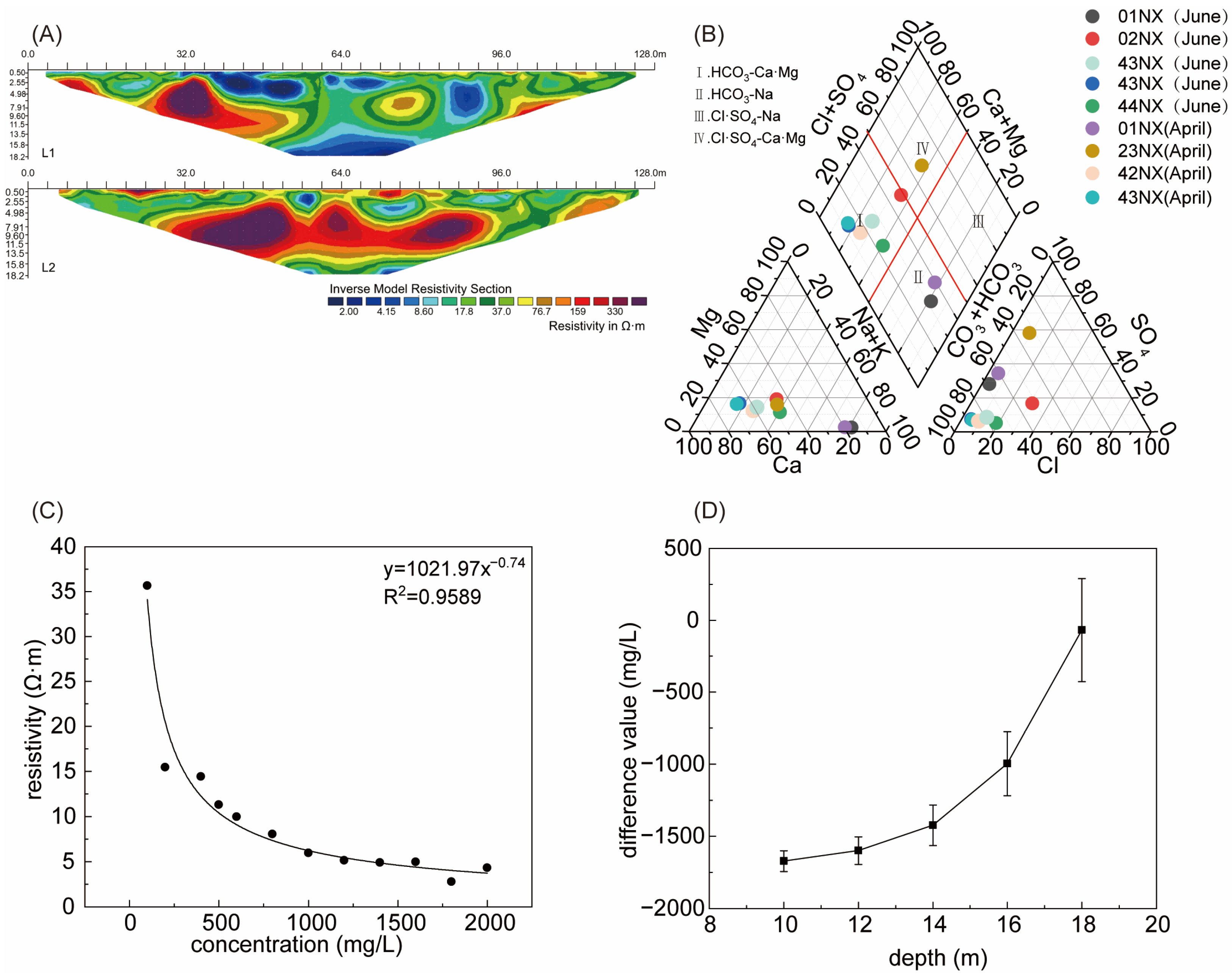
As shown in Figure 1A, the spatial layout of five sampling points (including 01NX (heavily contaminated) and 42NX (background)) and two ERT survey lines (L1 and L2) in the field achieved an accurate comparison between the core contamination area and the background area. The field ERT inversion results in Figure 2A showed that both L1 and L2 survey lines exhibited significant resistivity gradients: the central area of the survey line near the 01NX sampling point was a low-resistivity anomaly zone with a resistivity range of 0–110 Ω·m, while the central area of the survey line near the 42NX background sampling point was mostly a high-resistivity zone, with the upper-middle and middle-lower parts ranging from 15–100 Ω·m and the central part having a resistivity > 159 Ω·m. This clear spatial differentiation of resistivity was clearly consistent with the contamination/background attributes of the sampling points, initially confirming that ERT technology can effectively identify the spatial distribution characteristics of nitrate contamination plumes, laying a foundation for subsequent accurate interpretation combined with hydrochemical data.

It is worth noting that the resistivity difference between the nitrate-contaminated area and the background area (with a nitrate concentration difference of approximately 1800 mg/L) was significant. This result was similar to the research results of ERT survey lines measured by Gasperikova et al. in the Valley and Ridge physiographic province of the Appalachians, where the resistivity ratio corresponding to different nitrate concentrations at a subsurface depth of 4–14 m was comparable [9]. However, both studies required high nitrate concentrations to clearly determine the location of contaminants. This comparison clearly revealed the weak electrical response characteristic of nitrate, which makes it difficult to form high-resistivity zones at low concentrations like non-soluble organic pollutants [33]. This also essentially explains the limitation of traditional field ERT technology in directly and accurately identifying nitrate contamination—the weak electrical signal is easily masked by the complex hydrogeological conditions of the site [34]. Therefore, cross-validation with hydrochemical analysis data is required to improve the reliability of contamination identification.

The hydrochemical data of the field water samples collected in April and June (Figure 2B) provided key evidence for the cause of ERT resistivity anomalies: the water sample from the 01NX sampling point (with a nitrate concentration of approximately 1900 mg/L) belonged to the HCO₃-Na type, with nitrate-related ions as the main conductive components; while the water sample from the 42NX background sampling point (with a nitrate concentration of approximately 10 mg/L) belonged to the HCO₃-Ca-Mg type, with background bicarbonate as the main conductive ions. The significant differentiation between the two hydrochemical types provided specific evidence for the cause of ERT low-resistivity anomalies [35]. The proportion of nitrate-related ions in the water sample from the 01NX contamination point was significantly higher than that of other components, while the water sample from the 21NX background point was dominated by background bicarbonate ions. This corresponding relationship locked the intrinsic connection between the decrease in resistivity and nitrate contamination, effectively separating the interference of other soluble ions on the electrical signal and improving the targeting of contamination identification.

3.1.2. Establishment of Quantitative Response Relationship and Field Application Verification

To overcome the subjectivity and ambiguity dominated by experience in the interpretation of ERT, controlled experiments were carried out based on the Miller box apparatus shown in Figure 1C to establish a quantitative response model between resistivity and nitrate concentration. The goal was to realize the accurate quantitative delimitation of the nitrate contamination range after obtaining the ERT inversion image [14]. The fitting results showed a significant power function correlation between the two variables: y = 1021.97x^−0.74 (R² = 0.9589), where y is the resistivity (Ω·m), and x is the nitrate concentration (mg/L) (Figure 2C). The quantitative relationship with a high fitting degree (R² > 0.95) provided key experimental evidence for the quantitative interpretation of field ERT data, laying a foundation for the indirect inversion of nitrate concentrations under complex field conditions.

This quantitative relationship was applied to the ERT data of the L1 survey line of the field (at 64 m on the horizontal axis) to calculate the theoretical nitrate concentrations at different depths, which were then compared with the measured concentrations at the 01NX sampling point (Figure 2D). The results showed that the error exhibited significant depth dependence: in the deep layer (16–18 m), the difference between the theoretical and measured values approached zero, while in the shallow layer (8–14 m), the difference reached −1500 mg/L. This difference was due to the uniform formation medium, stable hydrogeological conditions, and few interfering ions in the deep layer (16–18 m), which were consistent with the hypothetical premise of the resistivity-nitrate concentration quantitative model [36]. Therefore, the deviation between the theoretically calculated value and the measured value was extremely small. The shallow layer (8–14 m) was affected by medium heterogeneity, the interface between the saturated and unsaturated zones of groundwater, mixed conduction of multiple ions, and the detection resolution of ERT. In addition, part of the nitrate existed in an adsorbed state and could not be monitored by resistivity, leading to a significant deviation between the theoretical and measured values [37]. On the other hand, the long survey line had to cross a section of cement pavement, which introduced errors into the measured apparent resistivity values. Even after multiple iterations of inversion, the root mean square (RMS) error remained at 29%. The inevitable errors observed in the field ERT measurements also exemplify a long-standing limitation of geophysical methods in the environmental field. Unlike drilling, which enables the collection of actual water and rock samples, geophysical methods rely on inferences drawn from measured geophysical parameters. For this reason, such methods require the analysis of results from multiple survey lines to study concentration variations across a given area; quantitative concentration calculations based solely on the results of a single survey line are inherently lacking in precision. Meanwhile, the static ERT test in the Miller box was simulated in a controlled environment, highlighting the inherent differences between indoor and field scenarios. This may also be the reason for the error for the difference between the theoretical values calculated from ERT inversion maps at different burial depths and the actual values, and it also provides a reference basis for the depth correction of subsequent field ERT data.

3.2. Survey Line Layout Optimization and Boundary Effect Mitigation: Improving ERT Monitoring Accuracy

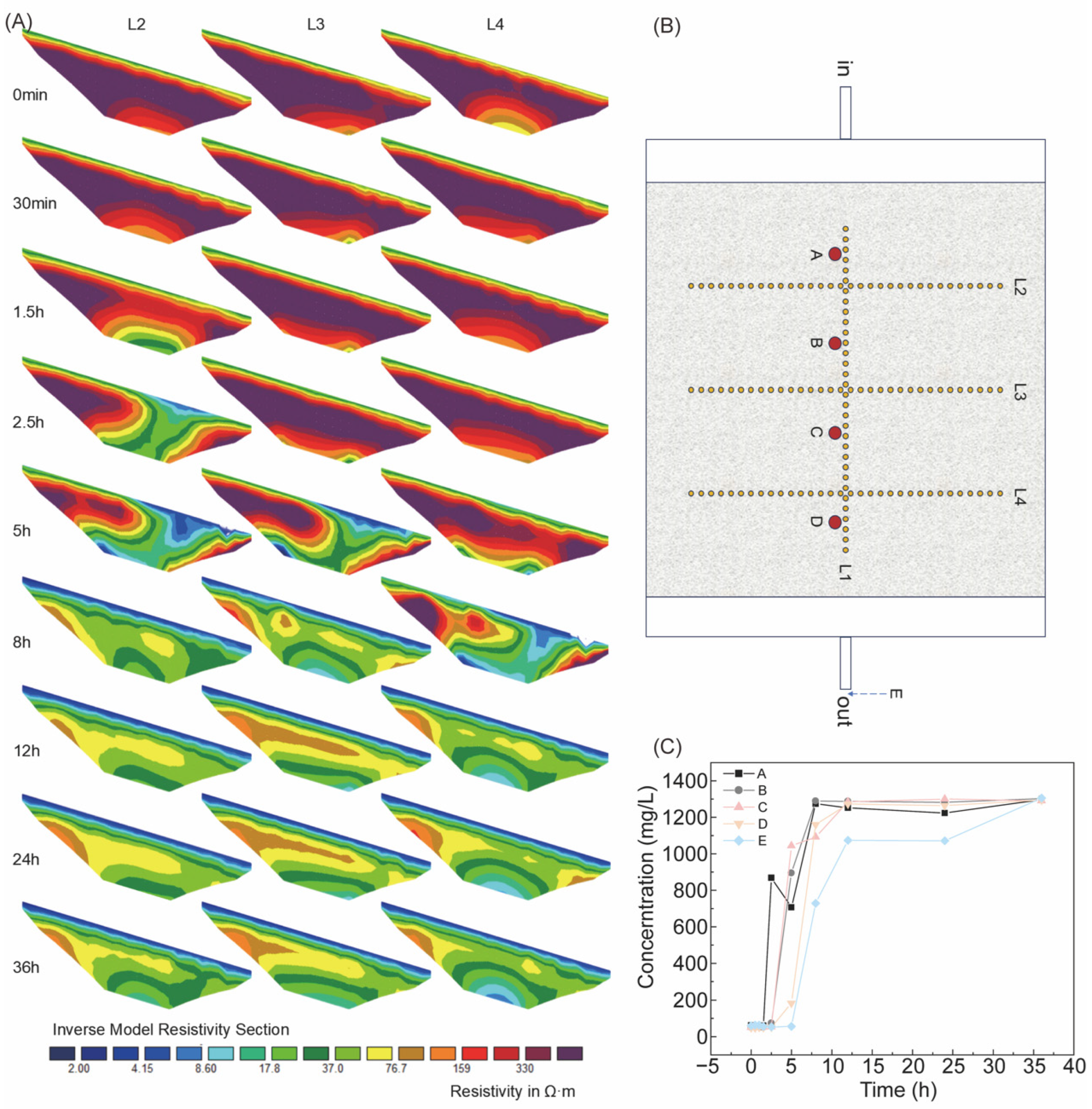
To address the problems of the limited scale of conventional ERT profiles, which makes it difficult to identify the weak electrical changes in nitrate, and the boundary effects in small-scale sand tank experiments that restrict monitoring accuracy [38,39], this study designed an optimized layout of “1 longitudinal main survey line L1 + 3 transverse auxiliary survey lines L2–L4” (Figure 3B). L1 was deployed along the water flow direction to track the longitudinal migration of contaminants; L2–L4 were uniformly deployed perpendicular to the water flow direction at intervals of 10 cm to capture the transverse diffusion range. Meanwhile, four sampling points (A, B, C, D) and an outlet sampling point E were set along the L1 survey line to realize the synchronous verification of ERT inversion results and measured concentrations.

Optimization Value of Multi-Line Layout: Full-Dimensional Characterization of Spatiotemporal Migration of Contamination Plumes

The multi-line ERT inversion results in Figure 3A and Figure 4 clearly showed the spatiotemporal evolution process of nitrate migration: at the initial stage of the experiment (0 min, saturated with background water), the entire sand tank was in a high-resistivity state (>330 Ω·m); 30 min after the injection of 01NX contaminated water, a low-resistivity zone (17.8–37.0 Ω·m) appeared in the upper reaches of L1, corresponding to the start of the increase in nitrate concentration at point A (Figure 3C, ~63 mg/L); at 5 h, the low-resistivity zone extended to the middle of the sand tank along L1, and synchronous low-resistivity signals appeared in the middle of the auxiliary survey lines L2–L3, indicating the transverse diffusion of nitrate. At this time, the concentration at point B rose to ~1000 mg/L; at 36 h, the low-resistivity zone covered the entire L1 and extended to the lower reaches of L4, and the concentration at the outlet point E stabilized at ~1200 mg/L.

The results confirmed that the multi-line layout effectively overcame the dimensional limitation of traditional single-line ERT, which can only reflect one-dimensional changes. The transverse diffusion range of nitrate was delimited by the auxiliary survey lines L2–L4 and the response time difference between L1 and L2–L4, avoiding the overestimation of the contamination plume range. This is impossible to achieve with traditional single-line monitoring or borehole point sampling, providing a reliable experimental basis for the prediction of contamination plume migration in the field.

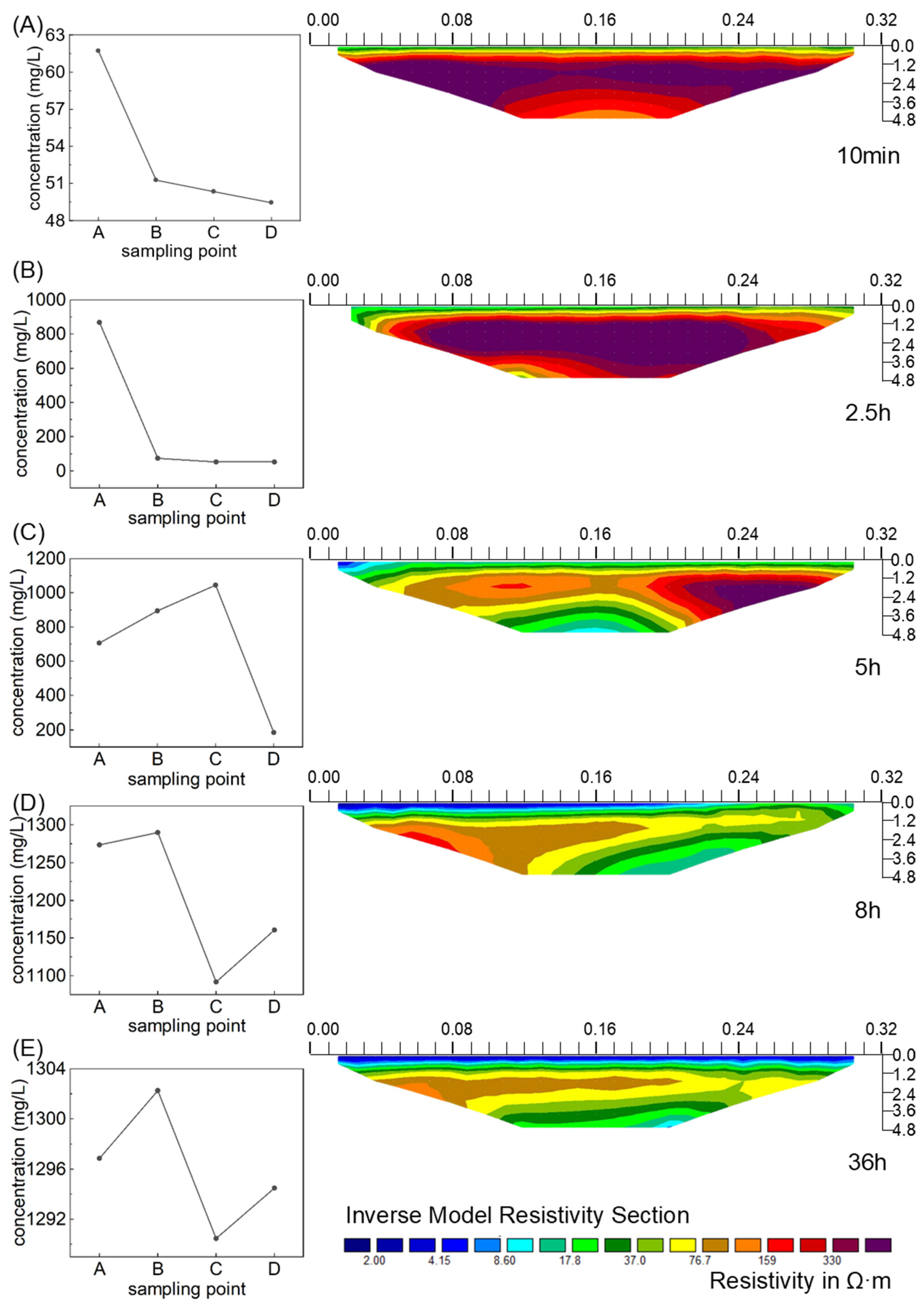
Figure 4 further focused on the main survey line L1, presenting the dynamic coupling relationship between ERT inversion results at different times and the corresponding nitrate concentrations at points A, B, C, and D: at 10 min, the local low-resistivity zone in the upper reaches of L1 (resistivity ~4.15 Ω·m) was synchronized with the increase in concentration at point A (~63 mg/L); at 2.5 h, the low-resistivity zone advanced downstream along L1, consistent with the time of the peak concentration at point A (~1000 mg/L). After 5 h, the low-resistivity zone gradually covered the entire survey line, and the concentrations at points C and D increased sequentially (~1000 mg/L at point C at 5 h, about 1150 mg/L at point D at 8 h). At 36 h, the resistivity of the L1 survey line was uniformly distributed, and the concentrations at all sampling points stabilized at around 1300 mg/L.

This triple matching of time–space–concentration not only verified the accurate tracking ability of the L1 main survey line for the longitudinal migration process of nitrate but also eliminated the interference of small-scale boundary effects through the sand tank experiment. Through reasonable survey line layout and sampling point setting, the influence of the boundary high-resistivity shadow zone and current field attenuation zone was reduced, expanding the effective testing area from the center of the tank to the entire tank. This provides an optimized experimental design scheme for simulating field contamination processes in small-scale experiments.

The multi-line layout strategy verified by the sand tank experiment provides a directly scalable technical framework for field ERT monitoring [40]. Based on overlapping electrode and parallel data acquisition technologies, this strategy significantly improves the accuracy of anomaly identification while ensuring monitoring efficiency through the optimized spatial configuration of survey lines and data association methods. In actual field monitoring, main survey lines can be systematically deployed along the groundwater flow direction, and continuous profile data can be used to track the migration path and dynamic evolution trend of nitrate contamination plumes. For the core contamination area, auxiliary survey lines can be densely deployed perpendicular to the water flow direction, and the cross-validation effect of multi-line data can be used to accurately delimit the transverse diffusion boundary and concentration gradient distribution of contaminants [41]. This combined layout of main survey line tracking and auxiliary survey line densification not only effectively makes up for the shortcomings of traditional field ERT, such as insufficient survey line density and limited ability to identify weak electrical response signals of nitrate. It enhances the signal-to-noise ratio of weak signals through multi-line data superposition, solving the problem that single survey lines are easily affected by background noise. It also successfully avoids the spatial representativeness deviation of traditional borehole sampling, which uses points to represent areas, realizing the leap from discrete point monitoring to continuous surface imaging. Combined with the non-invasive advantage of ERT technology, this layout can quickly cover a large monitoring area without damaging the integrity of the field medium, and simultaneously obtain the spatial distribution characteristics and migration laws of nitrate contamination. This provides efficient and reliable technical support for the precise management of contaminated sites and the formulation of remediation plans.

3.3. ERT Monitoring of Remediation Systems: Coupling Between Electrical Responses and Biogeochemical Processes

3.3.1. Regulatory Effect of Water Level Conditions on ERT Responses

To link the large-scale monitoring needs of nitrate contamination at the field scale with the refined management goals of remediation processes, grouped experiments were carried out based on the sand tank apparatus shown in Figure 1B. First, the multi-line layout strategy was used to accurately identify the migration trend and diffusion boundary of the contamination plume. Then, spherical soil samples containing different functional components (the initial soil samples were collected from the Sichuan site) were placed in the middle of the sand tank. ERT technology was used to simultaneously capture the migration of contaminants and the transport and diffusion dynamics of remediation agents and microorganisms. This design realized the transition from “spatial distribution monitoring” of field contamination to “key process visualization” of remediation processes, providing further feasibility verification for the precise remediation and effect evaluation strategies of nitrate contamination in the field.

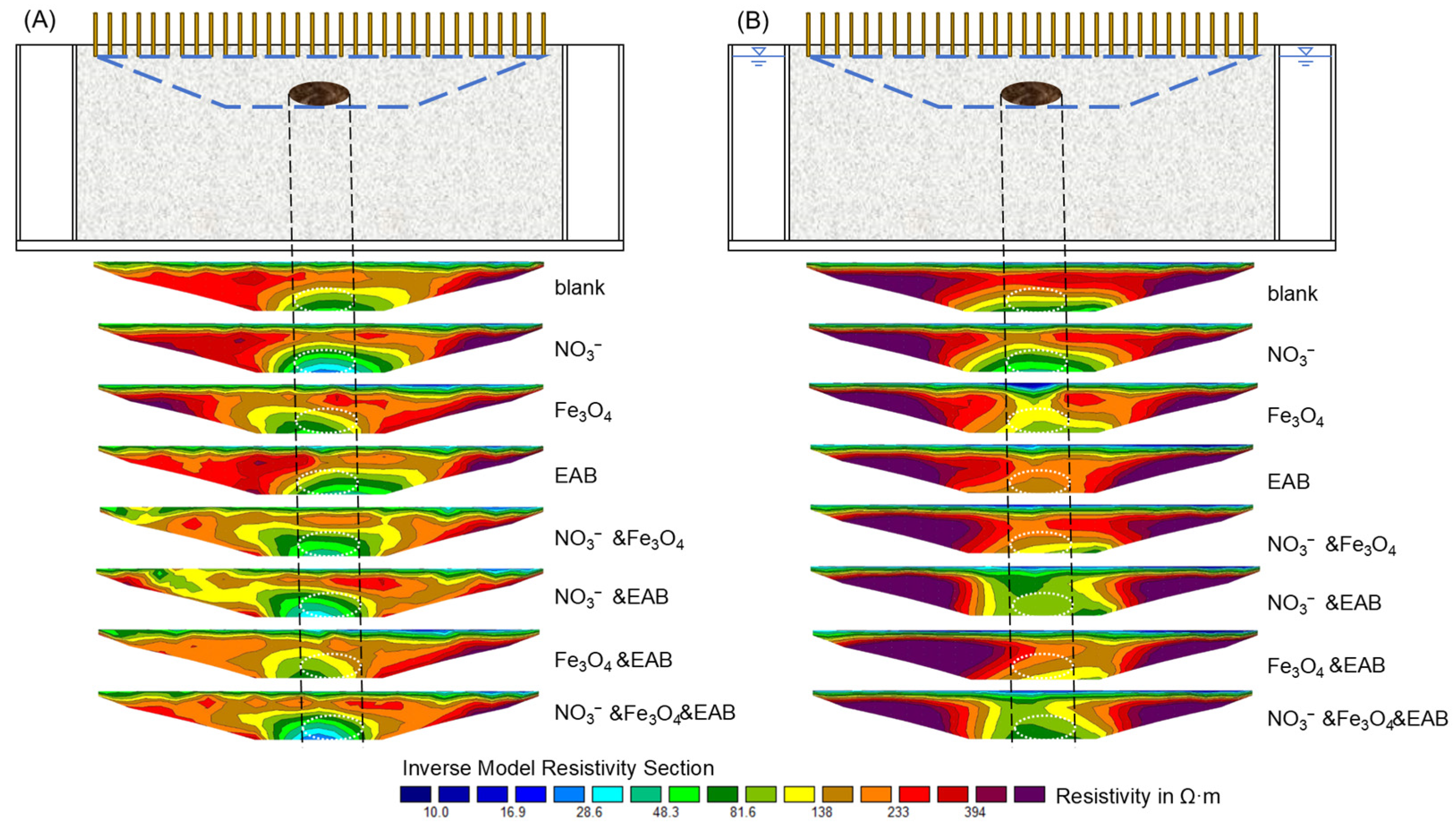
The results showed that water level conditions had a decisive influence on ERT responses (Figure 5): under low-water level conditions, compared with the blank group, the ERT profiles of the high-nitrite contamination group all showed obvious low-resistivity anomalies. However, the effects of other treatment groups could not exceed those of the high-concentration nitrate group, but there were still certain differences in the resistivity of the initial soil sample area. This indicated that under low-water levels, the contact between functional components and pore water was insufficient [42], biogeochemical reactions were difficult to occur [33], and ion migration was hindered [43], making it impossible to form an identifiable electrical gradient. Under high-water level conditions, the blank group showed a red/orange high-resistivity zone (138–394 Ω·m) and a small low-resistivity zone, representing the background electrical reference of the sand tank medium. Among the single-component groups, the group containing NO₃⁻ (nitrate) showed a green low-resistivity zone, the group containing Fe₃O₄ (magnetite) only slightly reduced the resistivity, and the low-resistivity zone of the group containing EAB (electroactive bacteria) was more concentrated (microbial metabolism enhanced ion migration). Among the two-component combinations, the low-resistivity zone range of NO₃⁻&Fe₃O₄ was larger than that of single NO₃⁻, and the green low-resistivity signal of NO₃⁻&EAB was more significant (the superposition of ion and microbial effects). The low-resistivity zone of Fe₃O₄&EAB was concentrated around the soil sample (with a better effect than single EAB). The three-component combination (NO₃⁻&Fe₃O₄&EAB) had the largest coverage of blue-green low-resistivity zones and the strongest conductivity among all groups. In summary, the resistivity characteristics of ERT signals were directly related to the type and combination mode of functional components. Combinations containing NO₃⁻, EAB and multi-component synergy exhibited more significant ERT low-resistivity signals, indicating that it is feasible to use ERT to monitor the transport and diffusion processes of remediation agents and microorganisms and to reveal the coupling relationship between electrical changes and biogeochemical reactions.

3.3.2. Electrical Response Mechanism of Functional Component Coupling

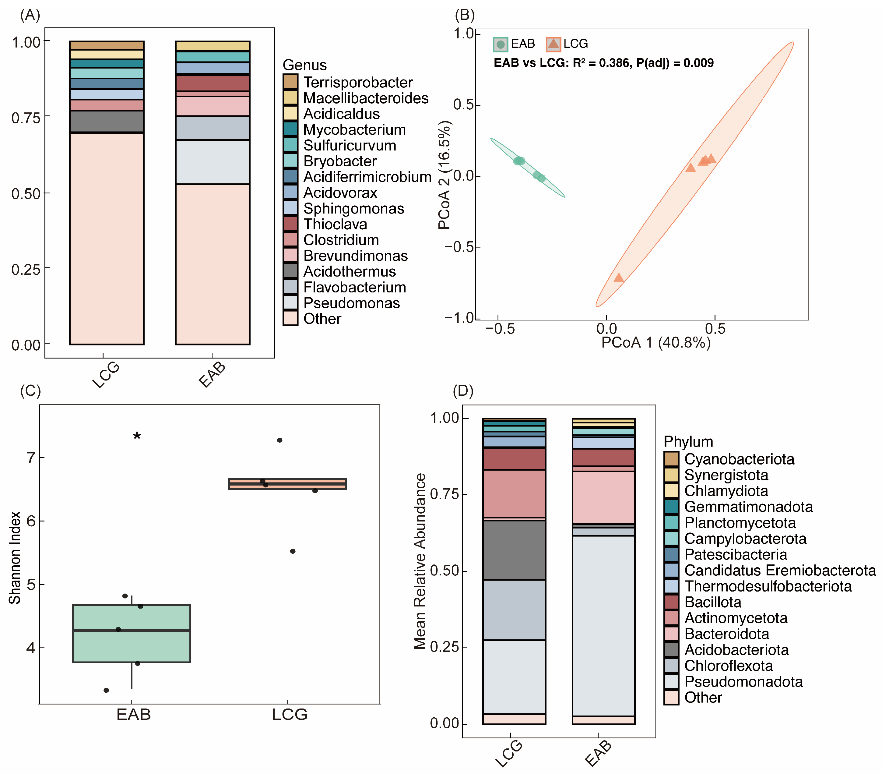
As illustrated in Figure 6, according to PCoA analysis of community beta diversity, with PCoA1 (explaining 40.8% of the variance) and PCoA2 (explaining 16.5% of the variance) as the axes, the sample points of the EAB group and the LCG group were completely separated. Pairwise PERMANOVA analysis confirmed a statistically significant difference in microbial community structure between the EAB and LCG groups (R² = 0.386, p = 0.009). Biological interpretation: An R² value of 0.386 indicates that the dissimilarity between EAB and LCG accounts for 38.6% of the total variation in microbial communities, demonstrating that the observed differentiation is not only statistically significant but also possesses substantial biological relevance. The microbial community diversity (richness and evenness) of the LCG group was higher, while the community structure of the EAB group was simpler. Due to additional current acclimation, there were significant and comprehensive differences in the microbial abundance characteristics between the two groups. The indices of the EAB group were concentrated in the 4–5 interval, while those of the LCG group were concentrated in the 6–7 interval, clearly showing that the microbial community diversity of the EAB group was much lower than that of the LCG group. Among the unique microbial taxa of the EAB group, some were directly related to conductivity and electron transfer processes. Synergistota at the phylum level could synergistically metabolize with electrogenic bacteria to assist electron transfer [44], while Pseudomonas at the genus level was a typical electroactive bacterium (EAB) that could realize electricity generation and conductivity through extracellular electron transfer [45]. Flavobacterium could secrete conductive extracellular polymeric substances [46], Brevundimonas was involved in Fe(III)/Mn(IV) reduction accompanied by electron transfer [47], and Acidovorax could use insoluble electron acceptors to complete extracellular electron transfer [48]. All these taxa were directly involved in conductivity-related processes. Thioclava produced ionic products through sulfur metabolism [49], and Sulfuricurvum participated in the sulfur cycle to generate ionic metabolites [50]. Both indirectly improved medium conductivity. These electroactive microorganisms, unique to the EAB group, were the microbial mechanisms underlying its stronger ERT low-resistivity electrical response in the sand tank experiment.

Comprehensive analysis of microbial data, different added components, and their ERT response relationships showed that this response difference originated from “chemical-biological” synergy. Weak response of single components: the NO₃⁻ group only slightly reduced resistivity through ion dissolution, the Fe₃O₄ group contributed a weak signal relying on its own conductivity, and the EAB group had low metabolic activity without nitrate substrates. None of them could form strong electrical anomalies. Synergistic gain of two components: in the NO₃⁻&Fe₃O₄ group, magnetite might act as an electron medium to accelerate the chemical reduction in nitrate and promote ion release. In the NO₃⁻&EAB group, the extracellular conductivity of EAB could reduce the resistivity of the area where EAB was located and improve the ERT response effect. In the NO₃⁻&EAB&Fe₃O₄ group, magnetite further improved the electron transfer efficiency of EAB, enhanced denitrification reactions, and might simultaneously promote the formation of a three-dimensional conductive network between biofilms and magnetite, resulting in a significant decrease in resistivity. The possible mechanisms are as follows: Construction of the conductive network: Fe₃O₄ nanoparticles embedded in the EAB biofilm act as an electronic highway, which establishes a direct electron transfer (DET) pathway and remarkably reduces the electron transfer resistance between bacterial cells and the extracellular electron acceptor (NO₃⁻). Acceleration of extracellular electron transfer (EET): Fe₃O₄ facilitates electron shuttling via the redox cycle of Fe²⁺/Fe³⁺. Serving as an active intermediate, it accepts electrons from EAB and rapidly donates them to NO₃⁻. Synergistic regeneration: In the NO₃⁻-EAB-Fe₃O₄ system, EAB biologically regenerates Fe²⁺ on the magnetite surface, which prevents the passivation of Fe₃O₄ and sustains an efficient electron transfer cycle [51]. This coupling effect constructed an electrical response chain of nitrate metabolism-ion release-conductive network, revealing the application potential of ERT signals and biogeochemical reactions in the remediation and monitoring of nitrate contamination [52].

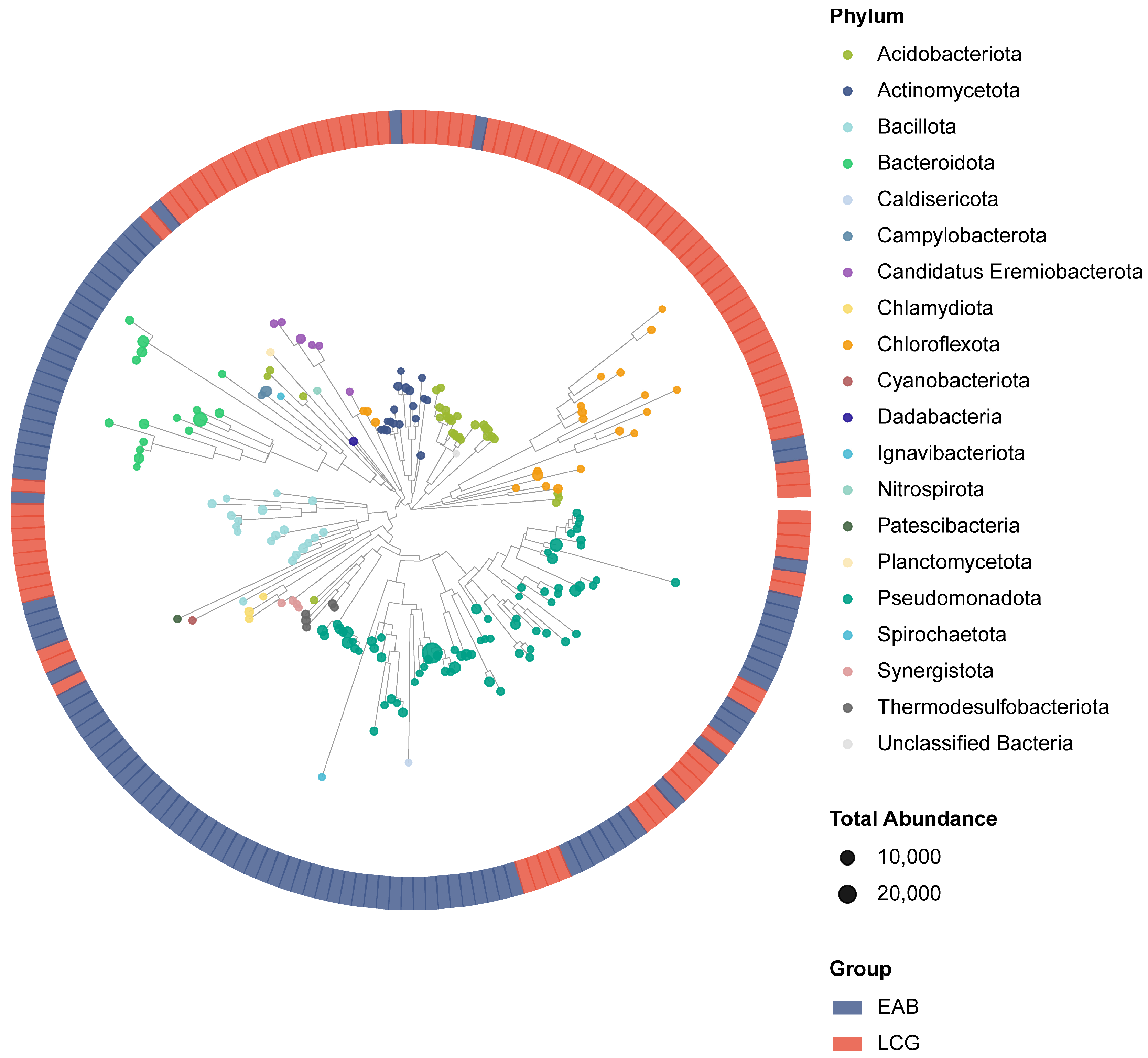
Species branches within the same group showed a cluster-like aggregation characteristic (e.g., the species branches of the EAB group were concentrated in the inner area corresponding to the dark blue block of the ring, while those of the LCG group were concentrated in the inner area corresponding to the red block), while species branches of different groups showed divergent separation. In the outer ring, the color distribution of EAB (dark blue segment) and LCG (red segment) showed almost no overlap, and each formed a continuous block aggregation. This intuitively reflected that the species affiliation of the two types of microbial communities had a strong group specificity. Most species were only enriched in one of the groups, and only a very few species branches were associated with the ring areas of both groups. This indicated that the difference in community composition was the core characteristic of the two types of microbial communities (Figure 7).

From the perspective of the correspondence between species abundance and classification: high-abundance nodes (corresponding to an abundance of 20,000) were mainly concentrated in phyla such as Bacteroidota, Chloroflexota, and Pseudomonadota, and the branches of these high-abundance species strictly extended to the ring areas of the corresponding groups (e.g., the high-abundance nodes of the Bacteroidota phylum, whose branches were almost all connected to the blue ring segment of the EAB group; the dominant species of the Pseudomonadota phylum were associated with both groups, but their branches still aggregated towards the blocks of EAB/LCG, respectively). Combined with the functions of these taxa, it can be seen that species of the Bacteroidota phylum mostly have the function of degrading refractory organic pollutants (such as the decomposition of complex carbohydrates and aromatic compounds). They can efficiently degrade complex organic matter, decompose difficult-to-utilize carbon sources such as polysaccharides, proteins, and mucoglycoproteins, and produce short-chain fatty acids (acetate, butyrate, etc.). These small-molecule organic acids are high-quality electron donors for electroactive microorganisms (such as Pseudomonas and Geobacter), which can significantly promote the extracellular electron transfer efficiency of EAB. Some Bacteroidota strains can secrete extracellular polymeric substances (EPS), which contain charged groups such as polysaccharides and proteins, and can improve medium conductivity [53]. Meanwhile, EPS can act as a biofilm skeleton to help EAB attach and colonize on the soil surface, promoting intercellular electron transfer (such as direct interspecies electron transfer, DIET). Species of the Pseudomonadota phylum include both taxa with electroactive respiration (such as extracellular electron transfer) (enriched in the EAB group) and taxa with anaerobic fermentation and pollutant transformation (partially enriched in the LCG group). This also explains why they are associated with both groups, but their branches aggregate directionally—the functional attributes determine their distribution in different microbial communities. This is the most direct function of Pseudomonadota related to your research. Its subordinate strains in multiple classes (such as Gammaproteobacteria and Betaproteobacteria) carry complete denitrification functional gene clusters (narG/nirS/nosZ, etc.). They can use nitrate (NO₃⁻) as an electron acceptor to sequentially reduce NO₃⁻ to NO₂⁻, NO, and N₂O, and finally convert it to N₂. They are key functional microbial communities for the in situ remediation of groundwater nitrate contamination. Meanwhile, its subordinate genera, such as Pseudomonas, Geobacter, and Shewanella, are all typical electroactive microorganisms (EAB), which can transfer electrons generated by metabolism to extracellular electron acceptors (such as magnetite, electrodes, nitrate, etc.) through extracellular electron transfer (EET) mechanisms [54]. Most taxa of Chloroflexota are typical oligotrophic microorganisms that can grow using low-concentration organic substrates (such as humus and refractory plant residues) and can obtain energy through metabolic pathways such as fermentation and hydrogen oxidation, which are perfectly adapted to the nutrient-poor environment in the field [55].

In addition, the branch distribution of low-abundance nodes (corresponding to an abundance of 10,000) in the figure also reflects this rule: although these low-abundance species (such as those of the Nitrospirota phylum) have low abundance, species of the Nitrospirota phylum have the function of nitrate redox (nitrification and denitrification). Their group-specific aggregation in both groups also corresponds to the functional differences between the EAB group (electrically assisted denitrification) and the LCG group (indigenous denitrification), further confirming that the structural differences between the two types of microbial communities are at the whole-community scale (not only limited to dominant species but also low-abundance species show group specificity), rather than the accidental distribution of local species. This figure not only shows the differences in community composition between EAB and LCG but also clearly presents the evolutionary and distribution characteristics of the two types of microbial communities, which form exclusive community structures through functional differentiation based on a common species pool, through details such as ring distribution of group-specific aggregation, functional directional enrichment of dominant species, and phylogenetic-functional coupling of branches. The EAB group is enriched with functional taxa for electroactive metabolism and electrically assisted pollutant transformation, while the LCG group aggregates functional taxa for organic matter degradation and natural nutrient cycling in the indigenous environment.

The experimental results of this section provide three key supports for field in situ remediation monitoring: the significant electrical response under high-water levels indicates that field remediation monitoring should select the saturated period of the aquifer for ERT detection to avoid signal distortion caused by low-water levels. The strong low-resistivity anomaly of the three-component system can be used as a direct criterion for the effective reaction of “remediation agents-microorganisms-contaminants”. If a similar low-resistivity signal is monitored in the field, it can be quickly judged that the remediation system has been successfully delivered to the target area and is functioning. The synergistic enhancement effect of magnetite and EAB provides an experimental basis for the optimal ratio of the field remediation system. Meanwhile, ERT can real-time track the diffusion range and reaction intensity of this synergistic system, providing technical support for the dynamic adjustment of remediation strategies.

4. Conclusions

Aiming at the monitoring challenges caused by the weak electrical response of nitrate contamination, this study systematically explored the application of ERT technology in nitrate pollution monitoring and remediation assessment through a combination of field investigations and laboratory experiments. The results showed that ERT technology can effectively identify the spatial distribution of nitrate plumes: the low-resistivity anomaly zones at the field scale were accurately consistent with the high-nitrate contaminated areas. Combined with Piper hydrochemical analysis, the interference from other ions could be excluded, thereby improving the targeting of pollution identification. The quantitative model between nitrate concentration and resistivity established via Miller box experiments provided a reliable basis for the quantitative interpretation of field ERT data. This model exhibited high application accuracy in the deep strata (16–18 m) with homogeneous media and minimal interference, while deviations were observed in the shallow strata (8–14 m) due to factors such as medium heterogeneity and multi-ion mixing. The layout strategy of “one longitudinal main survey line plus three transverse auxiliary lines”, verified by sand tank experiments, effectively overcame the dimensional limitations of traditional single-line ERT and the boundary effects of small-scale experiments. It enabled full-dimensional characterization of the spatiotemporal migration process of pollution plumes and quantitative calculation of migration rates. In addition, water level conditions and functional component combinations had a significant impact on ERT responses. Under high water level conditions, the ternary system of nitrate–magnetite–EAB exhibited the strongest low-resistivity response. Microbial analysis confirmed that the enrichment of electroactive groups in the EAB consortium was the core driving factor for enhanced electrical conductivity.

The findings of this study provide an important reference for the application of ERT technology in the monitoring and remediation of nitrate-contaminated groundwater, clarifying the key technical parameters and response mechanisms of ERT for identifying weak electrical response pollutants. The results demonstrate that the constructed integrated ERT technology system of field detection–laboratory modeling–remediation monitoring can successfully realize visual identification of nitrate plumes, quantitative inversion of concentrations, and dynamic tracking of remediation processes, making up for the shortcomings of traditional monitoring technologies such as low spatiotemporal resolution and strong subjectivity. Whether the proposed quantitative model and optimized survey line layout strategy are applicable to other types of weak electrical response pollutants under different hydrogeological backgrounds requires further research. Most chemical sites investigated in this study are covered with cement pavements. Owing to the interference of the thick, rigid cement pavements with high resistivity on the ground surface, the grid layout of multiple survey lines and high-precision detection could not be implemented, resulting in a relatively small number of survey lines employed in this study. In future research, if the surface detection conditions of the site are favorable, multiple survey lines parallel and perpendicular to the groundwater flow direction can be designed in a crossed arrangement, consistent with the sand tank experiment conducted in this study. Additionally, multiple representative wells can be selected at the site for borehole ERT measurements, and Miller box experiments can be carried out on drilling cores collected at different depths of the actual site. It is also feasible to design larger sand tanks to improve the detection depth of laboratory experiments; with the enhanced detection depth, stratified filling in the vertical direction and zonal filling in the horizontal direction can be implemented for detection in accordance with the formation heterogeneity of the actual site. Furthermore, several porous plastic pipes can be vertically inserted into the sand tank to simulate boreholes, for conducting injection experiments of contaminants and remediation agents. Borehole ERT detection in the sand tank can be supplemented as an auxiliary method, thereby realizing three-dimensional (3D) ERT detection within the sand tank. After the inversion images are spliced, high-precision full spatial coverage can be achieved. By systematically investigating the coupling relationship between ERT electrical responses and biogeochemical processes, this study deepens the understanding of the application potential of ERT in nitrate pollution monitoring and remediation. This achievement will facilitate the interpretation of ERT monitoring data from other similar contaminated sites and provide technical support for monitoring during in situ remediation for nitrate pollution in agricultural non-point sources and industrial sites.

References

1. Zhang, M.; Zhi, Y.; Shi, J.; Wu, L. Apportionment and uncertainty analysis of nitrate sources based on the dual isotope approach and a Bayesian isotope mixing model at the watershed scale. Sci. Total Environ. 2018, 639, 1175–1187. [Google Scholar] [CrossRef]
2. Xin, J.; Wang, Y.; Shen, Z.; Liu, Y.; Wang, H.; Zheng, X. Critical review of measures and decision support tools for groundwater nitrate management: A surface-to-groundwater profile perspective. J. Hydrol. 2021, 598, 126386. [Google Scholar] [CrossRef]
3. García-Aróstegui, J.-L.; Baudron, P.; Robles-Arenas, V.M. Sampling methods may drive short-term groundwater nitrate variability in an irrigated watershed connected to a coastal lagoon (Campo de Cartagena-Mar Menor, SE Spain). Sci. Total Environ. 2024, 912, 169188. [Google Scholar] [CrossRef]
4. Day-Lewis, F.D.; Mackley, R.D.; Bence, R. Sampling in Long-Screened Wells: Issues, Misconceptions, and Solutions. Groundwater 2024, 62, 669–680. [Google Scholar] [CrossRef] [PubMed]
5. Riwayat, A.I.; Nazri, M.A.A.; Abidin, M.H.Z. Application of electrical resistivity method (ERM) in groundwater exploration. J. Phys. Conf. Ser. 2018, 995, 012094. [Google Scholar] [CrossRef]
6. Benson, A.K.; Payne, K.L.; Stubben, M.A. Mapping groundwater contamination using dc resistivity and VLF geophysical methods—A case study. Geophysics 1997, 62, 80–86. [Google Scholar] [CrossRef]
7. Yan, Z.; Song, X.; Wu, Y.; Gao, C.; Wang, Y.; Yang, Y. Fingerprinting organochlorine groundwater plumes based on non-invasive ERT technology at a chemical plant. Appl. Sci. 2022, 12, 2816. [Google Scholar] [CrossRef]
8. Rucker, D.F.; Fink, J.B. Inorganic plume delineation using surface high-resolution electrical resistivity at the BC cribs and trenches site, Hanford. Vadose Zone J. 2007, 6, 946–958. [Google Scholar]
9. Gasperikova, E.; Hubbard, S.S.; Watson, D.B.; Baker, G.S.; Peterson, J.E.; Kowalsky, M.B.; Smith, M.; Brooks, S. Long-term electrical resistivity monitoring of recharge-induced contaminant plume behavior. J. Contam. Hydrol. 2012, 142–143, 33–49. [Google Scholar] [CrossRef]
10. Meng, F.; Wang, J.; Zhao, Y. Mapping and monitoring dense non-aqueous phase liquid source zone by fused surface and cross-borehole electrical resistivity tomography. J. Hazard. Mater. 2024, 478, 135618. [Google Scholar] [CrossRef]
11. Gao, W.; Xiang, C.; Wu, C.; Li, X.; Zhang, W.; Tang, L.; Jiang, J.; Li, W.; Guo, J.; Xue, S. Unveiling heavy metal(loid) contamination and migration at an abandoned smelting site: Integrated geophysical and hydrological analyse. Chem. Eng. J. 2024, 500, 156853. [Google Scholar] [CrossRef]
12. Tsai, Y.-J.; Chou, Y.-C.; Wu, Y.-S.; Lee, C.-H. Noninvasive survey technology for LNAPL-contaminated site investigation. J. Hydrol. 2020, 587, 125002. [Google Scholar] [CrossRef]
13. Park, S.; Yi, M.-J.; Kim, J.-H.; Shin, S.W. Electrical resistivity imaging (ERI) monitoring for groundwater contamination in an uncontrolled landfill, South Korea. J. Appl. Geophys. 2016, 135, 1–7. [Google Scholar] [CrossRef]
14. Robinson, J.; Johnson, T.; Rockhold, M. Feasibility assessment of long-term electrical resistivity monitoring of a nitrate plume. Groundwater 2020, 58, 224–237. [Google Scholar] [CrossRef]
15. Andersen, M.S.; Baron, L.; Gudbjerg, J.; Gregersen, J.; Chapellier, D.; Jakobsen, R.; Postma, D. Discharge of nitrate-containing groundwater into a coastal marine environment. J. Hydrol. 2007, 336, 98–114. [Google Scholar] [CrossRef]
16. Wehrer, M.; Binley, A.; Slater, L.D. Characterization of reactive transport by 3-D electrical resistivity tomography (ERT) under unsaturated conditions. Water Resour. Res. 2016, 52, 8295–8316. [Google Scholar] [CrossRef]
17. Adepelumi, A.; Solanke, A.; Sanusi, O.; Shallangwa, A. Model tank electrical resistivity characterization of LNAPL migration in a clayey-sand formation. Environ. Geol. 2006, 50, 1221–1233. [Google Scholar] [CrossRef]
18. Adeniran, M.A.; Oladunjoye, M.A.; Doro, K.O. Electrical resistivity imaging of crude oil contaminant in coastal soils—A laboratory sandbox study. J. Appl. Geophys. 2024, 230, 105516. [Google Scholar] [CrossRef]
19. Sentenac, P.; Hogson, T.; Keenan, H.; Kulessa, B. Small scale monitoring of a bioremediation barrier using miniature electrical resistivity tomography. J. Appl. Geophys. 2015, 115, 24–31. [Google Scholar] [CrossRef]
20. Sentenac, P.; Montinaro, A.; Kulessa, B. Diesel transport monitoring in simulated unconfined aquifers using miniature resistivity arrays. Environ. Earth Sci. 2010, 61, 107–114. [Google Scholar] [CrossRef]
21. Mohammed Nazifi, H.; Gülen, L.; Gürbüz, E.; Pekşen, E. Time-lapse electrical resistivity tomography (ERT) monitoring of used engine oil contamination in laboratory setting. J. Appl. Geophys. 2022, 197, 104531. [Google Scholar] [CrossRef]
22. Lévy, L.; Thalund-Hansen, R.; Bording, T.; Fiandaca, G.; Christiansen, A.V.; Rügge, K.; Tuxen, N.; Hag, M.; Bjerg, P. Quantifying reagent spreading by cross-borehole electrical tomography to assess performance of groundwater remediation. Water Resour. Res. 2022, 58, e2022WR032218. [Google Scholar]
23. Cao, S.; Zhan, G.; Wei, K.; Zhou, B.; Zhang, H.; Gao, T.; Zhang, L. Raman spectroscopic and microscopic monitoring of on-site and in-situ remediation dynamics in petroleum contaminated soil and groundwater. Water Res. 2023, 233, 119777. [Google Scholar] [CrossRef] [PubMed]
24. Wei, K.-H.; Ma, J.; Xi, B.-D.; Yu, M.-D.; Cui, J.; Chen, B.-L.; Li, Y.; Gu, Q.-B.; He, X.-S. Recent progress on in-situ chemical oxidation for the remediation of petroleum contaminated soil and groundwater. J. Hazard. Mater. 2022, 432, 128738. [Google Scholar] [CrossRef]
25. Ma, X.; Zhang, J.; Schwartz, N.; Li, J.; Chao, C.; Meng, J.; Mao, D. Characterizing landfill extent, composition, and biogeochemical activity using electrical resistivity tomography and induced polarization under varying geomembrane coverage. Geophysics 2024, 89, E151–E164. [Google Scholar] [CrossRef]
26. Flores Orozco, A.; Williams, K.H.; Long, P.E.; Hubbard, S.S.; Kemna, A. Using complex resistivity imaging to infer biogeochemical processes associated with bioremediation of an uranium-contaminated aquifer. J. Geophys. Res. Biogeosci. 2011, 116. [Google Scholar] [CrossRef]
27. Mao, D.; Revil, A.; Hort, R.D.; Munakata-Marr, J.; Atekwana, E.A.; Kulessa, B. Resistivity and self-potential tomography applied to groundwater remediation and contaminant plumes: Sandbox and field experiments. J. Hydrol. 2015, 530, 1–14. [Google Scholar] [CrossRef]
28. Xia, T.; Ma, M.; Huisman, J.A.; Zheng, C.; Gao, C.; Mao, D. Monitoring of in-situ chemical oxidation for remediation of diesel-contaminated soil with electrical resistivity tomography. J. Contam. Hydrol. 2023, 256, 104170. [Google Scholar]
29. Kim, M.; Kim, S.; Yang, W.; Sim, J. Determination of nitrite and nitrate in postmortem whole blood samples of 10 sodium nitrite poisoning cases: The importance of nitrate in determining nitrite poisoning. Forensic Sci. Int. 2022, 335, 111279. [Google Scholar] [CrossRef]
30. Ding, H.; Su, J.; Sun, Y.; Yu, H.; Zheng, M.; Xi, B. Insight into spatial variations of DOM fractions and its interactions with microbial communities of shallow groundwater in a mesoscale lowland river watershed. Water Res. 2024, 258, 121797. [Google Scholar] [CrossRef]
31. Wang, S.; Wang, X.; Fessler, M.; Jin, B.; Su, Y.; Zhang, Y. Insights into the impact of polyethylene microplastics on methane recovery from wastewater via bioelectrochemical anaerobic digestion. Water Res. 2022, 221, 118844. [Google Scholar] [CrossRef]
32. Ruff, S.E.; Humez, P.; De Angelis, I.H.; Diao, M.; Nightingale, M.; Cho, S.; Connors, L.; Kuloyo, O.O.; Seltzer, A.; Bowman, S. Hydrogen and dark oxygen drive microbial productivity in diverse groundwater ecosystems. Nat. Commun. 2023, 14, 3194. [Google Scholar] [CrossRef]
33. Caterina, D.; Flores Orozco, A.; Nguyen, F. Long-term ERT monitoring of biogeochemical changes of an aged hydrocarbon contamination. J. Contam. Hydrol. 2017, 201, 19–29. [Google Scholar] [CrossRef] [PubMed]
34. Robinson, J.; Johnson, T.; Thomle, J.; Cambeiro, J.; Peta, K.; Jaysaval, P.; Mackley, R. Interpretation of large-scale, long-term electrical geophysical monitoring guided by a process simulation. Vadose Zone J. 2024, 23, e20303. [Google Scholar] [CrossRef]
35. Albuquerque, G.M.; Mansur, K.L.; Silva, G.C.; Mello, C.L.; Braga, M.A. Fault mapping and characterization of a coastal aquifer related to a mangrove ecosystem, using electrical resistivity tomography (ERT), ground penetrating radar (GPR) and hydrochemical data: The case of the Mangue de Pedra Aquifer, Armação dos Búzios, Brazil. J. S. Am. Earth Sci. 2022, 120, 104095. [Google Scholar]
36. Zhang, D.; Wang, P.; Cui, R.; Yang, H.; Li, G.; Chen, A.; Wang, H. Electrical conductivity and dissolved oxygen as predictors of nitrate concentrations in shallow groundwater in Erhai Lake region. Sci. Total Environ. 2022, 802, 149879. [Google Scholar] [CrossRef] [PubMed]
37. Tso, C.-H.M.; Kuras, O.; Wilkinson, P.B.; Uhlemann, S.; Chambers, J.E.; Meldrum, P.I.; Graham, J.; Sherlock, E.F.; Binley, A. Improved characterisation and modelling of measurement errors in electrical resistivity tomography (ERT) surveys. J. Appl. Geophys. 2017, 146, 103–119. [Google Scholar] [CrossRef]
38. Hung, Y.-C.; Lin, C.-P.; Lee, C.-T.; Weng, K.-W. 3D and boundary effects on 2D electrical resistivity tomography. Appl. Sci. 2019, 9, 2963. [Google Scholar] [CrossRef]
39. Moreira, C.A.; Rosolen, V.; Furlan, L.M.; Bovi, R.C.; Masquelin, H. Hydraulic conductivity and geophysics (ERT) to assess the aquifer recharge capacity of an inland wetland in the Brazilian Savanna. Environ. Chall. 2021, 5, 100274. [Google Scholar] [CrossRef]
40. Chen, X.; Yang, X.; Wu, X.; Cao, Y.; Yue, M.; Zhou, G. Three-dimensional observation system of direct current method based on overlapping electrodes and its application. Acta Geophys. 2025, 73, 1377–1392. [Google Scholar]
41. El-khteeb, A.; Mabrouk, W.M.; Soliman, K.S.; El Aguizy, O.M.; Metwally, A. Archeological exploration via integrated shallow geophysical methods: Case study from Saqqara, Giza, Egypt. npj Herit. Sci. 2025, 13, 38. [Google Scholar] [CrossRef]
42. Jodry, C.; Palma Lopes, S.; Fargier, Y.; Sanchez, M.; Côte, P. 2D-ERT monitoring of soil moisture seasonal behaviour in a river levee: A case study. J. Appl. Geophys. 2019, 167, 140–151. [Google Scholar] [CrossRef]
43. Deceuster, J.; Kaufmann, O.; Van Camp, M. Automated identification of changes in electrode contact properties for long-term permanent ERT monitoring experiments. Geophysics 2013, 78, E79–E94. [Google Scholar] [CrossRef]
44. Leong, L.E.; Denman, S.E.; Kang, S.; Mondot, S.; Hugenholtz, P.; McSweeney, C.S. Identification of the mechanism for dehalorespiration of monofluoroacetate in the phylum Synergistota. Anim. Biosci. 2023, 37, 396–403. [Google Scholar] [CrossRef] [PubMed]
45. Qi, X.; Wang, H.; Gao, X.; Zhang, L.; Wang, X.; Xu, P. Efficient power recovery from aromatic compounds by a novel electroactive bacterium Pseudomonas putida B6-2 in microbial fuel cells. J. Environ. Chem. Eng. 2022, 10, 108536. [Google Scholar] [CrossRef]
46. Lin, C.; Liang, H.; Yang, X.; Zhan, J.; Yang, Q. Voltage recovery from frozen microbial fuel cells in the laboratory and outdoor field reactors. Sci. Total Environ. 2024, 942, 173751. [Google Scholar] [CrossRef]
47. Sakr, E.A.; Khater, D.Z.; El-khatib, K.M. Electroactive Brevundimonas diminuta consortium mediated selenite bioreduction, biogenesis of selenium nanoparticles and bio-electricity generation. J. Nanobiotechnol. 2024, 22, 352. [Google Scholar] [CrossRef]
48. Fei, Y.; Zhang, B.; Zhang, Q.; Chen, D.; Cao, W.; Borthwick, A.G. Multiple pathways of vanadate reduction and denitrification mediated by denitrifying bacterium Acidovorax sp. strain BoFeN1. Water Res. 2024, 257, 121747. [Google Scholar] [CrossRef]
49. Mou, T.; Su, J.; Zhang, J.; Yu, L.-Y.; Chen, H.-H.; Zhang, Y.-Q. Thioclava kandeliae sp. nov., Isolated from the Rhizosphere Soil of Mangrove Plant Kandelia candel. Curr. Microbiol. 2025, 82, 200. [Google Scholar] [CrossRef] [PubMed]
50. Cron, B.; Henri, P.; Chan, C.S.; Macalady, J.L.; Cosmidis, J. Elemental sulfur formation by Sulfuricurvum kujiense is mediated by extracellular organic compounds. Front. Microbiol. 2019, 10, 2710. [Google Scholar] [CrossRef]
51. Jin, Y.; Zhou, E.; Ueki, T.; Zhang, D.; Fan, Y.; Xu, D.; Wang, F.; Lovley, D.R. Accelerated Microbial Corrosion by Magnetite and Electrically Conductive Pili through Direct Fe0-to-Microbe Electron Transfer. Angew. Chem. Int. Ed. 2023, 62, e202309005. [Google Scholar] [CrossRef] [PubMed]
52. Cruz Viggi, C.; Casale, S.; Chouchane, H.; Askri, R.; Fazi, S.; Cherif, A.; Zeppilli, M.; Aulenta, F. Magnetite nanoparticles enhance the bioelectrochemical treatment of municipal sewage by facilitating the syntrophic oxidation of volatile fatty acids. J. Chem. Technol. Biotechnol. 2019, 94, 3134–3146. [Google Scholar] [CrossRef]
53. Martin, H.; Rogers, L.A.; Moushtaq, L.; Brindley, A.A.; Forbes, P.; Quinton, A.R.; Murphy, A.R.; Hipperson, H.; Daniell, T.J.; Ndeh, D. Metabolism of hemicelluloses by root-associated Bacteroidota species. ISME J. 2025, 19, wraf022. [Google Scholar] [CrossRef]
54. Chobert, S.-C.; Roger-Margueritat, M.; Flandrin, L.; Berraies, S.; Lefèvre, C.T.; Pelosi, L.; Junier, I.; Varoquaux, N.; Pierrel, F.; Abby, S.S. Dynamic quinone repertoire accompanied the diversification of energy metabolism in Pseudomonadota. ISME J. 2025, 19, wrae253. [Google Scholar] [CrossRef] [PubMed]
55. Freches, A.; Fradinho, J.C. The biotechnological potential of the Chloroflexota phylum. Appl. Environ. Microbiol. 2024, 90, e01756-23. [Google Scholar] [CrossRef] [PubMed]
Figure 1. Schematic diagram of field survey lines, sampling point distribution, and related experiments: (A) distribution of field survey lines (L1, L2) and groundwater sampling points (01NX and 42NX are background groundwater sampling points; 02NX, 23NX, 43NX, and 44NX are groundwater sampling points in the survey area); (B) schematic diagram of the Miller box experiment; (C) overall schematic diagram of the sand tank experiment.
Water 18 00404 g001
Figure 2. (A) Actual inversion results of field ERT survey lines L1 and L2; (B) piper trilinear diagram of hydrochemical data of field sampling points; (C) nitrate concentration and resistivity response curve based on the Miller box experiment in Figure 1C; (D) application of the quantitative relationship to ERT data of the L1 survey line—error results of the comparison between the calculated theoretical nitrate concentrations at different depths at 64 m on the horizontal axis and the measured concentrations at the 01NX sampling point.
Water 18 00404 g002
Figure 3. (A) ERT inversion results of survey lines L2, L3, and L4 based on (B); (B) schematic diagram of the optimized multi-line layout strategy for the sand tank experiment (L1–L4); (C) measured line graph of nitrate concentrations at different sampling positions (A, B, C, D) at different time points in (B).
Water 18 00404 g003
Figure 4. (AE) ERT inversion results of the L1 survey line synchronized with nitrate concentrations at points A, B, C and D in Figure 3B.
Water 18 00404 g004
Figure 5. ERT remediation monitoring of nitrate-contaminated groundwater in sand tank experiments: correlation diagram of response characteristics of 8 experimental ratios (background water/contaminated water/magnetite/electroactive bacteria single-factor and composite groups) under high and low water level conditions ((A)—low water level; (B)—high water level). Blue dashed lines indicate the detectable area; white dashed lines indicate the position of soil samples.
Water 18 00404 g005
Figure 6. Comparison of community characteristics between indigenous microorganisms and electroactive bacteria (EAB) based on 16S rRNA sequencing analysis: community structure, phylogenetic differentiation, and diversity characteristic analysis: (A) genus-level community structure composition and dominant species distribution characteristic diagram; (B) community phylogenetic differentiation diagram revealed by Bayesian PCoA analysis; (C) alpha diversity difference evaluation diagram mediated by the Shannon index,* indicates that p > 0.05; (D) phylum-level community structure composition and species classification statistical diagram.
Water 18 00404 g006
Figure 7. Phylogenetic tree diagram of microbial phylum-level classification: the outer ring is marked in red and blue, the size of branch labels represents abundance, and colors distinguish phyla.
Water 18 00404 g007