Real-Time Detection of River Contaminants Using Neural Networks: A Case Study of the Ebro River

Abstract

According to the UN World Water Development Report 2024, global food production has more than doubled over the past three decades, placing increasing pressure on freshwater systems due to climate change, urban expansion, and intensified pollution events. This study presents a Monitoring and Mitigation Framework (MMF) for real-time river contamination detection, contamination source identification, and estimation of Chemical Oxygen Demand (COD) concentrations at the source. The framework is based on Inverse Estimation (IE) algorithms using feed-forward neural networks trained on approximately 85,000 simulated pollution events for the Ebro River (Spain). Each event represents a 52 h contamination episode monitored at two locations with a 10 min sampling interval, covering a wide range of COD concentrations. For low-concentration scenarios (<1000 mg/L), the TensorFlow-based regression model achieved a Mean Absolute Relative Error (MARE) of 0.26% and a Mean Square Relative Error (MSRE) of 1.82%, while for higher concentrations (>1000 mg/L), the scikit-learn implementation provided superior performance with MARE below 1.85%. Source location identification achieved an accuracy of 81%, increasing to 97% when allowing adjacent river sections. Overall, the MMF is a scalable, low-cost, real-time decision-support tool for water authorities such as the Confederación Hidrográfica del Ebro (CHE) to detect, track, and mitigate pollution events.

1. Introduction

River contamination events caused by accidental spills or illegal discharges from agricultural, industrial, or urban activities continue to pose serious environmental, social, and economic risks worldwide. Unlike chronic pollution, these episodic events often evolve rapidly, making early detection and source identification essential for minimizing ecological damage and supporting timely mitigation actions by water authorities [1,2].

In large river systems, contamination management is further complicated by hydrodynamic variability, limited monitoring infrastructure, and the time lag between pollutant release and downstream detection. As a consequence, pollution events are frequently identified only after significant dispersion has occurred, reducing the effectiveness of corrective measures and hindering the attribution of responsibilities [3,4].

Chemical Oxygen Demand (COD) is widely used to characterize organic pollution from agricultural and industrial sources, as elevated COD levels are directly linked to oxygen depletion, ecosystem degradation, and risks to downstream water uses. Recent studies emphasize the relevance of COD as an operational variable for pollution monitoring and early-warning systems, particularly under high-load and transient contamination scenarios [5,6].

Several high-impact contamination events reported in recent decades have exposed the limitations of conventional monitoring approaches in major river basins, reinforcing the need for integrated tools capable of detecting pollution in near real time while simultaneously identifying its origin and estimating pollutant loads [7,8]. In the absence of timely mitigation measures, elevated pollutant loads can trigger significant ecological deterioration in aquatic systems [9,10].

In this context, the development of scalable and cost-effective monitoring frameworks that combine limited sensor data with advanced data-driven techniques has become a priority for river basin authorities. Despite the growing interest in artificial intelligence for water systems, one of the main limitations of real-time AI applications remains the scarcity of pilot-scale implementations and long-term datasets capable of capturing unsteady operational conditions. Recent studies highlight that this lack of representative, high-frequency data significantly constrains the development and validation of AI-based monitoring tools in real-world water environments [11]. To address these limitations, this study proposes a Monitoring and Mitigation Framework (MMF) based on neural networks trained on an extensive set of simulated contamination scenarios, explicitly designed to operate under highly unsteady hydraulic and pollution conditions in large river systems, such as the Ebro River.

Over the past decades, surface water bodies have been repeatedly affected by both accidental and deliberate pollutant releases across different regions worldwide. Notable examples include the chemical spill of 4-methylcyclohexane methanol into the Elk River (USA) in 2014 [12], as well as prolonged mercury contamination episodes associated with industrial activity in the Ebro River (Spain) during the late twentieth century [13], as well as chronic contamination associated with mining activities in resource-exhausted areas [14].

In this sense, recurrent contaminant scenarios have been reported in the Ebro River during long periods of time, according to ref. [15], which reports that, between 1986 and 1987, the Ebro River annually transported between 9000 and 12,000 tonnes of particulate carbon, along with 1200 to 1400 tonnes of particulate nitrogen, 300 to 2000 tonnes of particulate phosphorus, and between 87,000 and 165,000 tonnes of suspended solids into the sea.

Reducing the environmental consequences of such events requires rapid source localization together with reliable quantification of pollutant concentrations. In riverine and drainage networks influenced by agricultural, industrial, and urban activities, delayed detection often results in irreversible ecological damage. Consequently, the ability to identify contamination at its origin plays a decisive role in supporting timely intervention measures and safeguarding aquatic ecosystems.

In this context, MMF is designed to support real-time source localization and concentration estimation across river networks. The framework facilitates the analysis of contamination evolution at identified COD concentrations at pollution hotspots. This framework was previously tested on contamination scenarios in a reach of the Llobregat River [16], yielding remarkable results. However, new challenges have emerged when evaluating the MMF in a different context. In particular, the Ebro River represents a longer and more complex system, with greater flow variability and a broader range of pollution scenarios. According to the Confederación Hidrográfica del Ebro (CHE), an autonomous body under the Ministry for the Ecological Transition and the Demographic Challenge (MITECO), these characteristics required a thorough reassessment and adaptation of the MMF to meet the specific conditions and requirements of the Ebro River.

2. Methodology

MMF was designed to reduce the impact of contaminant discharges by locating the origin of pollution and estimating the temporal evolution of COD concentrations at those sources. While initially conceived for application in riverine environments, the MMF is also capable of operating in real time, integrating high-frequency data from water quality and hydraulic sensors installed throughout the river or drainage network. This section presents the methodology used to develop and deploy the MMF system.

2.1. Foundations and Structure of the MMF Methodology

To achieve the objectives of the Monitoring and Mitigation Framework (MMF), a set of task-oriented algorithms was developed, each addressing a specific function within the overall workflow. The conceptual organization of the framework, illustrated in ref. [16], supports the analysis of river and drainage networks by integrating hydrodynamic characterization, scenario generation, and data-driven inference.

The framework combines the extraction of geometric and hydraulic information from the river system with the generation of a synthetic database of contamination events. This database provides the basis for training inverse estimation models, which are subsequently applied to infer the most probable source locations and to reconstruct the temporal evolution of COD concentrations at identified points of interest.

A concise description of each functional component is provided below, while implementation details are available in the Supplementary Materials.

2.2. Methodological Framework of the IE Algorithms

Within the MMF, the Inverse Estimation (IE) algorithms constitute the core analytical component, as they are responsible for identifying the most likely location of contamination sources and reconstructing the temporal evolution of COD concentrations at those locations. In the Ebro River application, particular emphasis was placed on ensuring that the IE algorithms remained robust under conditions of high hydrodynamic variability and limited monitoring information.

The development of the IE component integrates three complementary elements: (i) the systematic generation of physically consistent contamination scenarios, (ii) the construction of a comprehensive learning database capturing a wide range of hydraulic and water quality conditions, and (iii) the training and validation of data-driven models capable of mapping sparse sensor observations to source characteristics. The specific implementation of these elements for the Ebro case is described in the following subsections.

2.2.1. LMS Algorithm and SWMM Simulation

The LMS algorithm was developed to generate enough and different pollution scenarios (combining flow and contamination transport boundary conditions) to build the Learning Database, so all scenarios generated by the algorithm could be attributed to real contamination events in our study cases at the Ebro River.

To construct a learning dataset representative of realistic contamination events in a large river system, a Location–Magnitude Scenario (LMS) algorithm was implemented. The objective of the LMS algorithm is to systematically explore combinations of upstream flow conditions, contamination source locations, and initial COD concentrations that could plausibly occur in the Ebro River, thereby ensuring that all generated scenarios remain physically meaningful and consistent with observed hydrological behavior.

The definition of boundary conditions was guided by hydrological records, regulatory guidelines, and historical water quality assessments for the Ebro River reach between the Flix and Ribarroja reservoirs (17 km). According to the Ebro River Basin Authority [17], the minimum operational flow at the Flix reservoir is approximately 68 m³/s, while maximum average flows may reach 420 m³/s. Based on these records, flow conditions ranging from 50 to 450 m³/s were considered, discretized into 51 representative scenarios. Flow values above 500 m³/s were excluded, as extreme flood events tend to dilute point-source pollution, reducing the relative environmental impact of agricultural and industrial discharges.

Surface water COD concentrations in the Ebro River typically range between 10 and 160 mg/L, depending on the river section and local conditions [18], with urban and industrial discharges accounting for up to 71% of the total organic load. These concentration ranges are consistent with historical datasets reported by ref. [19] for the Ebro corridor downstream of Zaragoza, as well as with real-time measurements from the SAICA monitoring platform and the official report Monitoring of the Status of Water Bodies [20]. Additional ecological assessments conducted in this river reach further support these observations [21,22].

To evaluate the robustness of the MMF under extreme but plausible conditions, the LMS algorithm was nevertheless configured to generate COD concentrations spanning from 1 mg/L to 250,000 mg/L. Although these upper values exceed historical observations, their inclusion was intended to enhance the generalization capacity of the IE algorithms when confronted with rare, high-impact contamination events in large river systems. This configuration resulted in 2550 distinct COD concentration levels included in the Learning Database.

Potential contamination sources were distributed along the downstream 14 km of the study reach, where industrial facilities and agricultural activities are predominantly located. In total, 48 cross-sections were considered as candidate source locations, selected from the 120 cross-sections used to discretize the river geometry. Compared with previous applications of the MMF to the Llobregat River, the Ebro case involves substantially wider flow ranges, broader COD concentration intervals, and a larger number of potential contamination sources, leading to markedly increased variability and a more challenging inverse estimation problem [23].

All hydraulic and pollution scenarios generated by the LMS algorithm were simulated using the SWMM 5.1 software [24], which models unsteady flow and contaminant transport along the river reach.

(a)

Flow Governing Equations

The conservation of mass and momentum for unsteady free surface flow through a channel or pipe are known as the St. Venant equations and can be expressed as:

$$\begin{gathered} {\displaystyle \frac{\partial A}{\partial t}}+{\displaystyle \frac{\partial Q}{\partial x}}=0 \\ {\displaystyle \frac{\partial Q}{\partial t}}+{\displaystyle \frac{\partial \left(Q^2/A\right)}{\partial x}}+gA{\displaystyle \frac{\partial H}{\partial x}}+gA{S}_f=0 \end{gathered}$$

(1)

In the governing equations, the spatial coordinate and time are denoted by x and t, respectively, while the flow cross-sectional area is represented by A. The discharge is expressed as Q, and the hydraulic head within the conduit is defined as the sum of the channel invert elevation and the local water depth. Flow resistance effects are accounted for through the friction slope S_f, and gravitational acceleration is represented by g [25].

These equations correspond to the one-dimensional formulation of open-channel flow commonly adopted in hydraulic modeling. For steady and gradually varied conditions, the friction slope can be parameterized using the Manning formulation, which relates energy losses to channel roughness and hydraulic geometry:

$$S_f={\displaystyle \frac{n^{2}Q\left|U\right|}{A{R}^{4/3}}}$$

(2)

where n denotes the Manning roughness coefficient and R is the hydraulic radius of the flow cross section. The inclusion of the absolute discharge value ensures that the resistance term consistently acts opposite to the flow direction, regardless of the sign of Q.

Equations (1) and (2) represent the one-dimensional Saint-Venant formulation coupled with a Manning-based friction law, which assumes predominantly longitudinal flow, hydrostatic pressure distribution, and gradually varied hydraulic conditions. These assumptions are consistent with the characteristics of the studied Ebro River reach, which presents a low slope, smooth geometric variations, and regulated flow conditions.

(b)

Transport Governing Equations

The longitudinal transport of dissolved substances in conduits and open channels can be represented through a one-dimensional mass balance formulation. This expression accounts for advective transport driven by the mean flow velocity, dispersive spreading along the flow direction, and source or sink processes associated with chemical or biological reactions, as stated by ref. [26]:

$${\displaystyle \frac{\partial c}{\partial c}}=-{\displaystyle \frac{\partial uc}{\partial x}}+{\displaystyle \frac{\partial }{\partial x}}\left(D{\displaystyle \frac{\partial c}{\partial x}}\right)+r(c)$$

(3)

where c denotes the solute concentration, u represents the longitudinal flow velocity, D is the dispersion coefficient, and r(c) accounts for reactive processes. In the SWMM implementation, hydrodynamic and transport calculations are performed in a sequential manner using a time-marching scheme, rather than through a fully coupled solution of the governing equations. The resulting flow and concentration fields are recorded at each time step and subsequently incorporated into the Learning Database used for training and validation of the inverse estimation models.

2.2.2. Learning Database

The Learning Database was constructed from approximately 85,000 SWMM simulations covering all combinations of the boundary conditions defined for the Ebro River case. Each simulation represents a distinct contamination event characterized by a specific source location, upstream flow condition, and initial COD concentration.

For each event, COD concentrations were recorded every 10 min at two monitoring locations along the river reach over a total duration of 52 h, resulting in 625 variables per simulation. This duration was selected to ensure that contamination plumes originating upstream could be fully captured at the downstream monitoring point. The 10 min sampling interval reflects the operational constraints of commercially available online COD sensors [27] and provides a realistic representation of field monitoring conditions. As no permanent water quality sensors are currently deployed in the studied Ebro River reach, all measurement data were generated using the SWMM simulation framework.

Despite the increased spatial extent and hydrodynamic complexity of the Ebro River case, the number of COD monitoring locations was deliberately limited to two, consistent with previous case studies. This design choice was motivated by two factors: first, to rigorously assess the robustness of the IE algorithms under sparse sensing conditions; and second, to reflect realistic economic and operational constraints associated with large-scale sensor deployment. These conditions substantially increase the difficulty of the inverse problem and therefore provide a stringent test of the proposed framework.

The IE component consists of two complementary data-driven models: a classification model designed to identify the most probable contamination source location and a regression model aimed at estimating the temporal evolution of COD concentrations at that source. Both models were developed using supervised machine learning techniques and trained and tested using the Learning Database generated for the Ebro River case.

Supervised learning techniques were adopted to construct predictive models from data, enabling the extraction of relationships between input variables and target outputs without relying on explicitly defined physical rules; see [28].

In the present case study, a supervised learning strategy was selected because the available dataset provides labeled examples, allowing each set of input features to be directly associated with a corresponding output response.

Although recurrent architectures such as Long Short-Term Memory (LSTM) networks are commonly applied to time-series modeling problems, temporal dynamics in this study are explicitly embedded in the input representation rather than handled through recurrent structures. Each sample in the Learning Database represents a complete contamination event and contains the full temporal evolution of COD concentrations over a 52 h period, recorded at two monitoring locations with a 10 min resolution.

As a result, each input vector consists of 625 time-ordered variables that collectively encode the temporal behavior of the system, enabling feed-forward neural networks to learn temporal dependencies directly from the data. Preliminary tests with recurrent architectures using reduced versions of the dataset were also conducted during the model development phase. However, these approaches required substantially higher computational costs and longer training times, without providing a noticeable improvement in the considered performance indicators.

The inverse estimation algorithms were finally implemented using artificial neural networks, ANN (MLP), to develop two complementary models. One model addresses a classification task focused on identifying the most likely contamination source location, while the second model performs a regression task aimed at estimating the temporal evolution of COD concentrations at that source.

To evaluate the performance of the regression and classification models, different sets of metrics were employed. Regression accuracy was quantified using the Mean Absolute Error (MAE), Mean Squared Error (MSE), Mean Square Relative Error (MSRE), and Mean Absolute Relative Error (MARE). For the classification task, standard evaluation measures, including accuracy, precision, recall, and the F1 score, were adopted.

The computational requirements for training the ANN models correspond to those of a standard workstation (Intel Core i7 CPU, 32 GB RAM) without GPU acceleration. Training was performed offline and required approximately 48 h for the regression model and 24 h for the classification model. Once trained, model deployment involves only forward inference and can be efficiently executed on CPU hardware.

Both final models were developed based on the Ebro case, and their performance was analyzed using the Llobregat case as a benchmark, employing different machine learning libraries. The steps introduced to generate the algorithms are as follows:

(A)

Training and Test Data

The dataset was divided into training and testing subsets using a hold-out validation strategy. Several experiments were conducted by varying the proportion of data assigned to each subset, with training ratios ranging from 70% to 80% and testing ratios from 20% to 30%. For the classification task, the best performance was obtained using a 75–25% split between training and testing data. In contrast, the regression models achieved optimal results with an 80–20% division, which was consistently adopted in the corresponding test cases.

(B)

Regression and Classification algorithms

Given the inherent complexity of simulating hydraulic behavior and pollutant transport in river reaches, multiple neural network architectures were evaluated. After testing several configurations (1-2-3-4 layers), a three-layer structure was selected for both classification and regression models in the Ebro case, as it offered the optimal balance between computational efficiency and predictive accuracy [29,30]. The regression network consists of three hidden layers with 256, 128, and 32 neurons, respectively, all using ReLU activation functions.

The activation function, which determines whether a neuron is activated based on the assigned weights, introduces the necessary nonlinearity into the learning process. Among the activation functions considered, the Rectified Linear Unit (ReLU) produced the most accurate and stable results in both modeling approaches to predict the temporal evolution of COD concentrations at the contamination source. Training was performed using the Adam optimizer (Google LLC, Mountain View, CA, USA) with a mean squared error (MSE) loss function over 750 epochs.

For the classification task, model development was performed using the Keras API with a TensorFlow backend (Google LLC, Mountain View, CA, USA), following established best practices in the literature [31]. In contrast, the regression model was initially implemented in TensorFlow, and subsequent iterations incorporated functionalities from the scikit-learn library to improve predictive performance.

The classification network is implemented as a feed-forward multilayer perceptron composed of three hidden layers with 128, 64, and 32 neurons, respectively. All hidden layers use the ReLU activation function, while the output layer employs a softmax activation function to estimate the probability distribution of the contamination source location. The model was trained using the Adam optimizer and the sparse categorical cross-entropy loss function for a total of 350 training epochs.

3. Results

3.1. Site Description and Testing Methodology

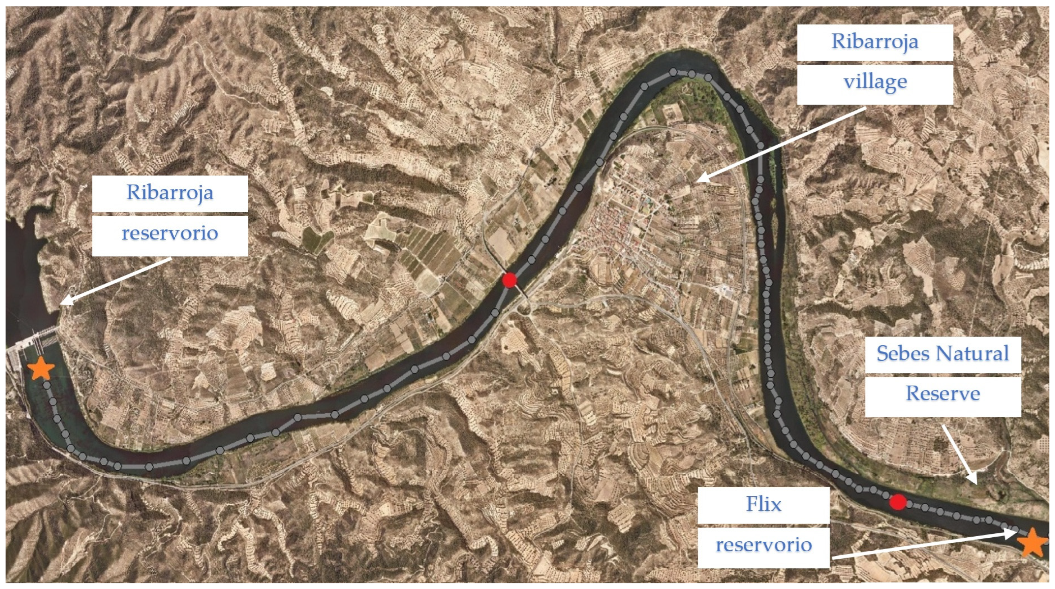
The Monitoring and Mitigation Framework (MMF) was trained and evaluated using a reach of the Ebro River. The selected case study covers the downstream 14 km segment of the river, as illustrated in Figure 1, and comprises a total of 120 cross-sections or computational nodes. Among these, 48 locations were considered as potential contamination sources based on their proximity to agricultural areas, industrial facilities, and urban drainage systems. The analysis focuses on these candidate source locations, with simulated COD concentrations ranging from 1 mg/L to 250,000 mg/L and river discharges between 50 m³/s and 450 m³/s.

Hypothetical COD sensors were assumed to operate at a 10 min sampling interval and were positioned at the Nautic Club Bridge and Mas Pitoia locations (Figure 1). In addition, a water level sensor was assumed at node 1 to represent sea-level influence, while a flow sensor was considered at the Old Hydraulic Laboratory location. All sensor measurements used in this study are synthetic and derived from hydrodynamic and transport simulations. Boundary conditions and operational scenarios were defined based on information available in the existing literature.

The IE algorithms were evaluated using two independent datasets: one derived from the original Learning Database and an additional dataset generated specifically to assess generalization performance. The latter dataset was produced under alternative boundary condition configurations to those used during training. In both cases, the data were obtained from SWMM-based simulations, as detailed in Section 2.

3.2. Regression Algorithm Test Case I

To assess how accurately the MMF predicts COD concentrations, a range of statistical error metrics were employed: MAE (Mean Absolute Error), MSE (Mean Squared Error), MSRE (Mean Squared Relative Error), and MARE (Mean Absolute Relative Error). MAE and MSE focus on absolute deviations between predicted and actual values, while MSRE and MARE provide a sense of the error in relative terms.

These metrics were computed under two conditions: (i) for the entire test dataset and (ii) for a subset of cases where COD concentrations remained below 1000 mg/L. The comparison between predicted and observed COD values over time at the pollution source, highlighting the performance of models trained with both the Scikit-learn and TensorFlow libraries. The results reflect consistently low error values across all 17,000 test instances.

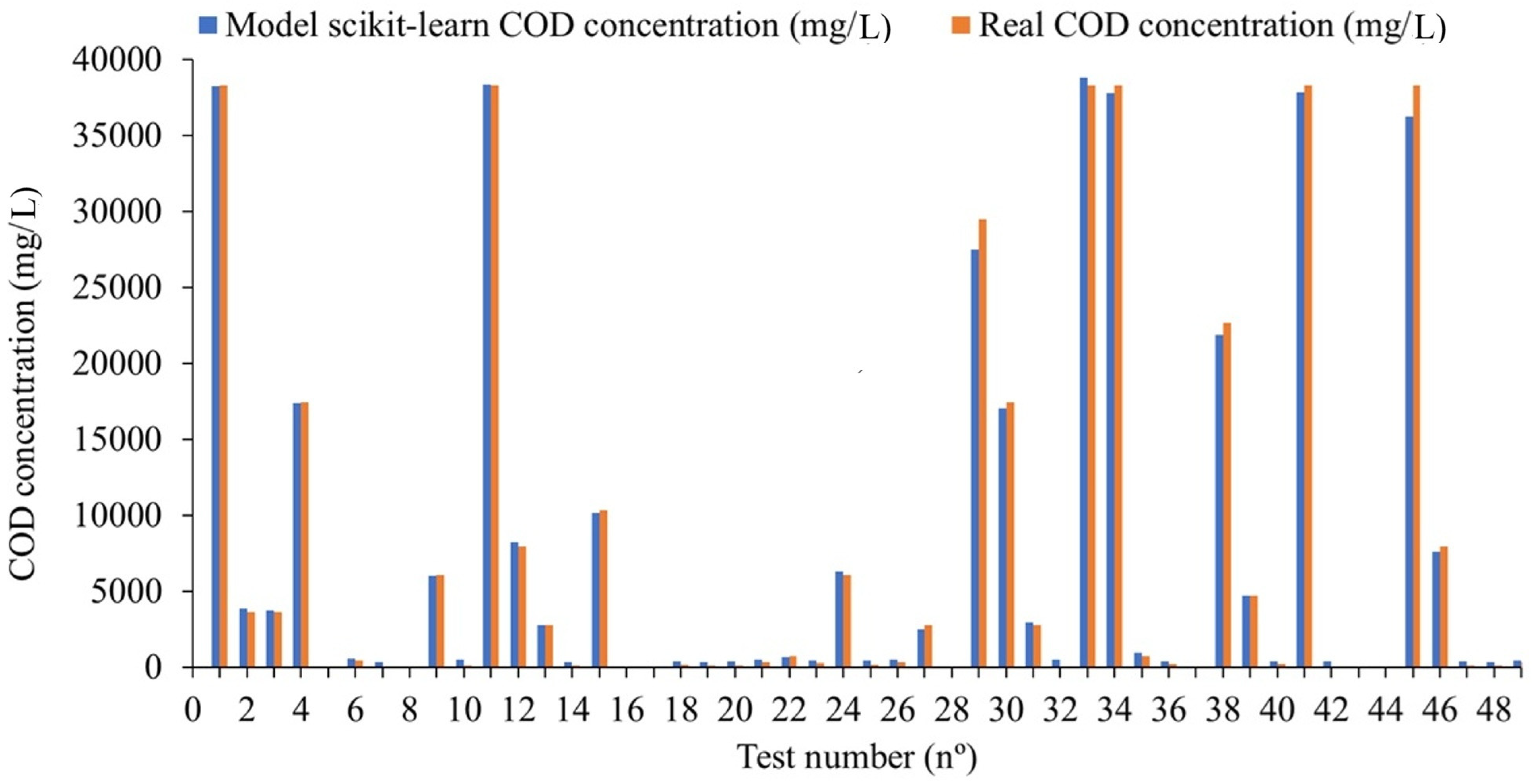
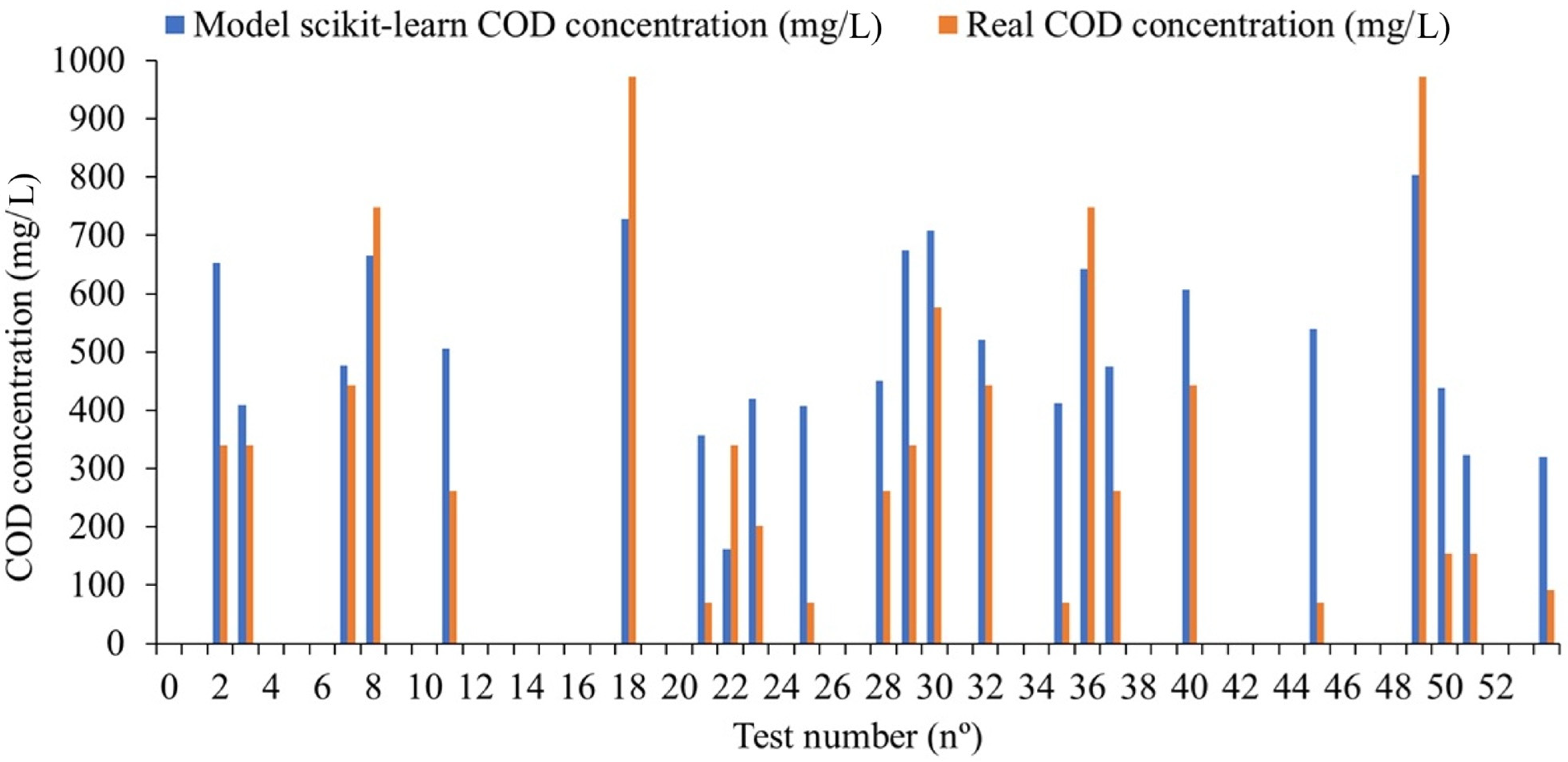
Furthermore, Figure 2 and Figure 3 present detailed results for the first 50 test cases obtained with Scikit-learn, while a full set of results is available in Supplementary Figure S5. Notably, the Scikit-learn-based algorithms yielded more accurate predictions than those developed using TensorFlow, especially for scenarios involving high COD concentrations. In this case, the model achieved consistently low prediction errors across the evaluated scenarios. In low-COD conditions (<1000 mg/L), the Mean Absolute Relative Error remained below 0.3%, with a minimum observed error close to zero. For high-COD scenarios (>1000 mg/L), the maximum Mean Absolute Relative Error remained below 1.85%, while the Mean Absolute Error stayed below 5000 mg/L even for concentrations up to 250,000 mg/L as shown in Table S3.

All non-relative error indicators (MAE and MSE) exhibited higher average errors compared to relative error indicators (MSRE and MARE), due to the fact that COD concentrations can reach up to 250,000 mg/L. In such cases, even small absolute errors are heavily penalized for high concentrations. The MSE values are particularly large in all scenarios because of the quadratic nature of this metric, where even minor percentage errors in high COD concentrations (e.g., >50,000 mg/L) result in large error values.

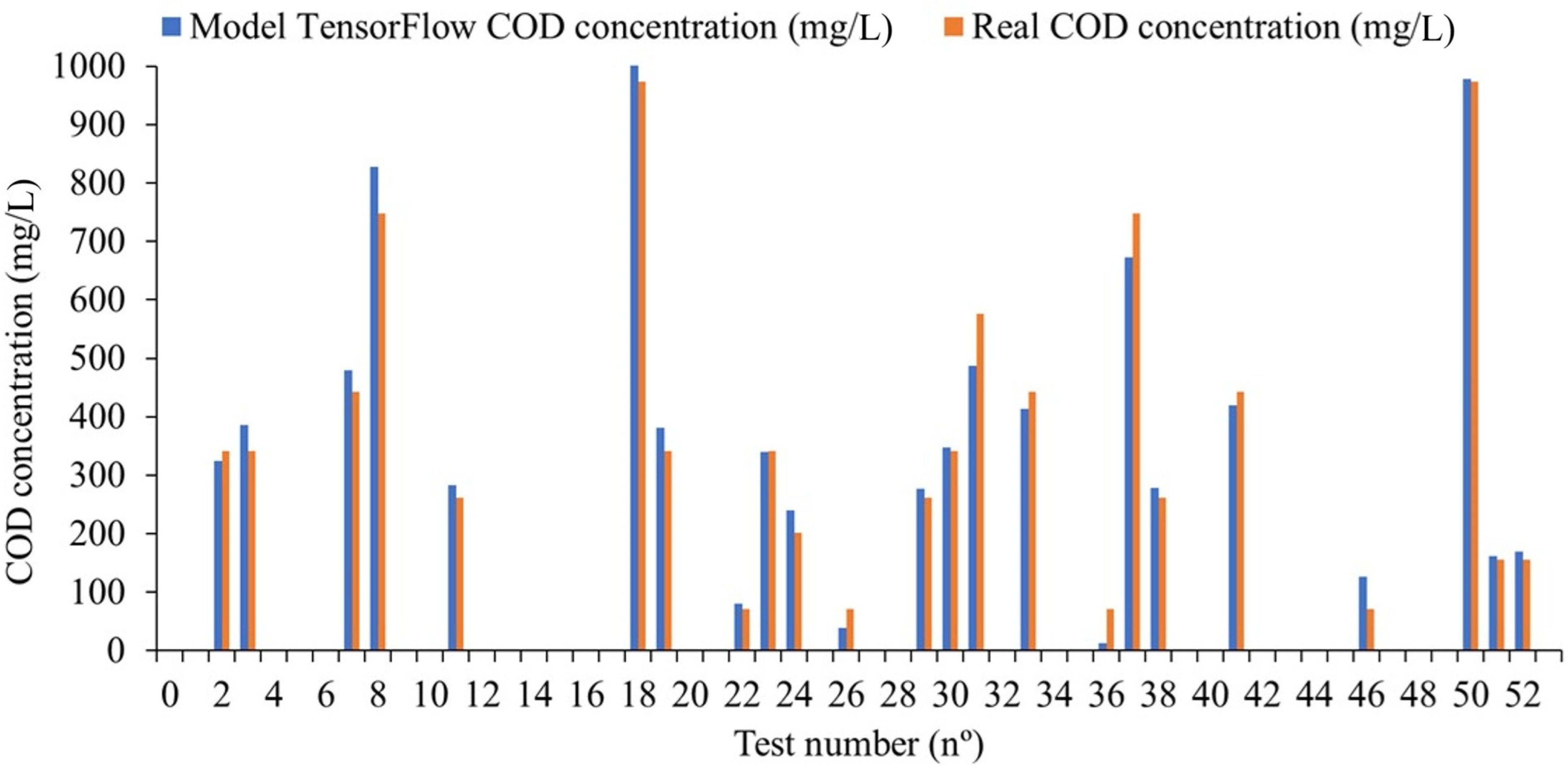
Conversely, when tests are limited to cases with COD concentrations below 1000 mg/L, average errors are significantly reduced,. Regarding model performance, Scikit-learn demonstrates better accuracy for COD concentrations over 1000 mg/L, as illustrated in Figure 4, where the model fits the real values. On the other hand, TensorFlow performs better for COD concentrations below 1000 mg/L. Figure 4 presents the results from TensorFlow for COD concentrations below 1000 mg/L, where TensorFlow shows a better overall fit than Scikit-learn. On the other hand, the MMF was also tested using a new dataset (Test Case II) that had not been used previously for training or testing the MMF (see Supplemental Materials).

Therefore, for the Ebro River case, it is strongly recommended to use both libraries in a complementary manner, that is, Scikit-learn for COD concentrations above 1000 mg/L and TensorFlow for those below this threshold.

3.3. Performance of the Classification Model for Test Case I

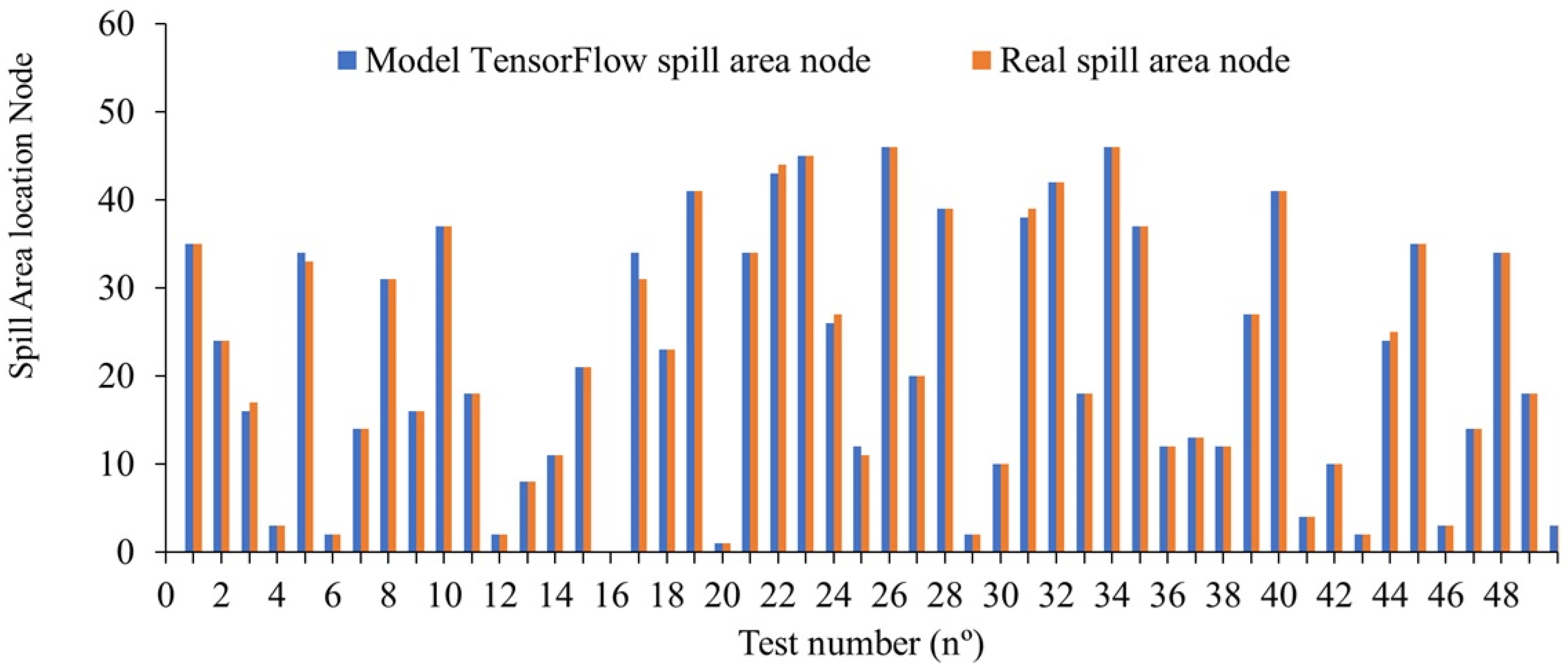
The performance of the inverse estimation classification model in Test Case I indicates a high level of accuracy across the evaluated scenarios. Out of the 21,250 test instances, a substantial number of contamination source locations were correctly identified. Model training was carried out using the TensorFlow framework, resulting in robust predictive behavior over the full set of cases.

Model predictions were compared against the known contamination source locations, and the results are summarized in Table S4. Classification accuracy was assessed using two complementary criteria. First, predictions were considered correct when the estimated source location exactly matched the true source position. Second, predictions falling within immediately adjacent upstream or downstream river sections were also treated as acceptable identifications. Regarding contamination source identification, the classification model correctly identified the exact source location in 81% of the test cases. When allowing one adjacent upstream or downstream river section, the identification accuracy increased to 97%. Precision, recall, and F1-score values ranged between 81% and 82%, indicating stable and robust classification performance across the evaluated scenarios; see Table S4.

The classification algorithm successfully identified a large number of COD concentration sources, as shown in Figure 5. Overall, the classification algorithm delivers highly reliable predictions for identifying point source contamination locations. On the other hand, the MMF was also tested using a new dataset (Test Case II) that had not been used previously for training or testing the MMF (see Supplemental Materials).

4. Analysis and Discussion

4.1. MMF: Robustness and Accuracy

Several methodologies have been proposed for predicting pollutant concentrations and identifying contamination sources in river systems. Physically based models, grounded in the advection–dispersion–reaction equation, can localize pollution sources accurately but often require extensive data such as dispersion coefficients, boundary conditions, and cross-sectional hydraulics and involve solving computationally demanding inverse problems (e.g., Bayesian or PSO methods).

To reduce complexity, hybrid methods have emerged. For example, ref. [32] introduced a geostatistical inverse framework to identify multiple point sources with fewer observations; while faster, it resulted in higher MAE and RMSE than MMF. Similarly, ref. [33] employed metaheuristic algorithms such as PSO, DE, and Metropolis–Hastings for source identification, achieving good localization but higher error levels in concentration estimations than MMF. Models integrating flow and water quality estimation through PSO or Muskingum routing [34,35] displayed faster runtimes but had elevated relative errors compared to MMF.

Parallel to these, data-driven approaches have grown. Long-term statistical models that relate pollution trends to land use or hydrological changes [3,36] are useful for retrospective analysis but do not enable real-time source identification. More recently, machine learning and IoT-enabled systems have shown promise for real-time water quality monitoring, combining sensor inputs (pH, turbidity, COD) with ML forecasts [37]. Nonetheless, these models often lack the dual capability to simultaneously identify source locations and estimate concentrations with transparency.

Emerging digital twin technologies provide comprehensive, real-time simulators of river basins, integrating AI, IoT, and hydraulic models such as [38,39]. While powerful for basin-wide management, they remain complex, data-intensive, and not tailored for minimal-input source tracking.

In contrast, the MMF combines simplicity and effectiveness: using two monitoring points and data-driven regression and classification, it reliably estimates both downstream concentrations and upstream source locations in real time. MMF avoids heavy physical modeling or inverse analysis while delivering high accuracy. This positions MMF as especially suitable for scalable deployment in complex river settings. The next paragraphs detail its robustness and precision in the Ebro vs. Llobregat case studies.

The MMF has demonstrated a high degree of robustness and accuracy, as evidenced by the results obtained in the Ebro River case study. These results are particularly noteworthy when compared with those previously obtained in the Llobregat River, offering strong support for the potential applicability of the method in varied hydrological contexts.

From a regression perspective, the relative error indicators (such as MSRE and MARE) yielded results that are closely aligned with those reported in the Llobregat case. Although absolute error metrics like MAE showed slightly less precision, the overall performance remains well within acceptable limits for practical environmental management in the studied reach of the Ebro.

In the case of the classification model, performance was even stronger. The accuracy, precision, recall, and F1 scores are highly consistent with those obtained in the Llobregat case, despite the fact that the Ebro scenario posed significantly greater challenges. Notably, both implementations relied on only two COD concentration monitoring points, but in the Ebro case the river reach was considerably larger (17 km compared to 8 km in the Llobregat case), and included far more potential contamination injection sections (48 potential cross-sections vs. 12 potential cross-sections in the Llobregat case). Additionally, the Ebro simulations covered a broader range of potential injection concentrations (1–250,000 mg/L vs. 1–120,000 mg/L) and a wider flow range (1.5–50 m³/s vs. 50–450 m³/s).

Furthermore, the robustness of the IE algorithms is supported by the fact that the hydraulic conditions of the Ebro reach are well-characterized thanks to prior studies conducted by the Barcelona School of Civil Engineering. In particular, parameters such as the Manning roughness coefficient were already precisely determined, eliminating the need for further calibration via optimization procedures [40].

These findings strongly suggest that the MMF, and the IE algorithms in particular, are viable for deployment in real-world river systems like the Ebro River, offering reliable environmental management tools in scenarios with greater complexity than the previously studied Llobregat case. In the case of the Ebro River, the MMF system could serve as a powerful tool to support environmental management tasks led by the Confederación Hidrográfica del Ebro (CHE), an autonomous body under the authority of the Ministry for the Ecological Transition and the Demographic Challenge (MITECO). This institution is responsible for monitoring water quality along the Ebro River, including critical areas such as Flix and the Ribarroja reservoir.

4.2. MMF Prediction for Real Time

Accurate and timely prediction of pollutant behavior in river systems is essential for effective environmental management, especially in contexts where industrial or urban discharges pose serious ecological risks. Several recent studies have demonstrated the feasibility of real-time or near real-time models for water quality forecasting in complex river systems.

One notable example is the work by ref. [41], who proposed an online adaptive learning algorithm capable of identifying the source location, discharge magnitude, and timing of pollution events in real time. This method leverages a neural network model updated continuously using incoming sensor data, making it especially well-suited for unsteady and non-stationary environments like rivers. The algorithm outperformed traditional optimization-based methods and showed robust generalization when deployed in synthetic pollution scenarios [41].

Similarly, ref. [42] developed a Random Forest-based classification system for the Marilao River in the Philippines, which achieved a 91.75% accuracy and a Kappa statistic of 0.81 when categorizing pollution levels using variables such as DO, BOD, and pH. Although not deployed in an online configuration, the system was designed to interface with IoT sensors, allowing for future integration into real-time water monitoring networks [42].

In another study, a predictive framework was applied to the Huangyang Reservoir in China [43], where traditional models such as ARIMA and LSTM were compared with modern long-term sequence forecasting models like Informer and LTSF-Linear. The LTSF-Linear model outperformed the others, reducing the Mean Squared Error (MSE) by 8.55% and the Mean Absolute Error (MAE) by 10.51%, demonstrating its advantage in short-term pollutant concentration forecasting. This study, conducted using an intensive deployment of monitoring devices, was published in Applied Sciences (2024) [43].

Due to the versatility of neural networks and their high computational speed, the MMF is not only useful for estimating COD concentrations at the contamination injection point and assessing whether an environmental crime has occurred, but also for identifying the responsible party. These capabilities make the MMF a valuable tool for deployment at the Sebes Nature Reserve in the Ebro River case, helping to monitor and control the surrounding environment. This is particularly relevant given the presence of several industrial facilities and agricultural systems located upstream of the Nature Reserve, between the Riba-roja and Mequinenza reservoirs.

Furthermore, once a contamination event has been detected by the MMF in the Sebes Nature Reserve, it becomes possible to simulate the travel time of the pollutant plume to the Nature Reserve and estimate the resulting COD levels upon arrival. This enables an assessment of the potential impact on the reserve’s flora and fauna and supports the implementation of timely mitigation measures.

5. Conclusions

The Monitoring and Mitigation Framework (MMF) proposed in this work exhibits excellent performance in detecting water pollution events, locating pollution sources, and estimating COD concentrations in river systems under realistic and variable conditions. At its core, the Inverse Estimation (IE) algorithms proved accurate and generalizable, achieving robust results even when applied to previously unseen test cases.

For COD concentration estimation, the Scikit-learn model outperformed TensorFlow in scenarios with high COD levels (above 1000 mg/L), achieving a Mean Absolute Relative Error (MARE) of 1.85% and a Mean Squared Error Relative (MSER) of 8.26% in Test Case I. Conversely, TensorFlow showed better performance in low-concentration events (below 1000 mg/L), with a MARE of 0.26% and MSER of 1.82% in Test Case I, highlighting the complementarity of both approaches depending on the pollution context.

The Mean Absolute Error (MAE) was also computed, with 229.3 mg/L for Scikit-learn and 56.52 mg/L for TensorFlow in the low-COD range in Test Case I. However, metrics like MSE are less informative in this scenario due to the high variability and scale of COD values: small relative errors in high-concentration cases can produce disproportionately large MSE values. For example, a 1% error in a 250,000 mg/L concentration translates into a 5000 mg/L squared deviation, inflating the MSE despite good predictive performance. Therefore, relative metrics such as MSER and MARE are preferred and more representative of the model’s behavior.

In terms of pollution source location, the TensorFlow classifier showed excellent generalization. In Test Case I, it identified the exact pollution source with 81% accuracy and reached 97% accuracy when including immediately upstream or downstream sections as acceptable matches. Precision, recall, and F1-score all reached 81–82%, and these results were confirmed in Test Case II in the Supplementary Materials.

In summary, MMF is a robust, low-cost, and real-time tool for environmental agencies such as the Confederación Hidrográfica del Ebro (CHE). It enables timely identification of pollution events and responsible actors, facilitating rapid and informed mitigation actions to protect water quality and aquatic ecosystems.

From a practical perspective, the proposed MMF is particularly suitable for regulated river reaches where monitoring infrastructure is sparse and rapid decision-making is required. The methodology is well adapted to applications involving early detection of accidental or illegal pollution events, real-time source localization, and operational support for river basin authorities.

Future research will focus on the integration of the framework with real sensor data as monitoring networks are progressively deployed, as well as on extending the approach to additional water quality parameters and river systems. Further developments may also explore alternative machine learning architectures and data fusion strategies to enhance performance under more complex hydrodynamic and monitoring conditions.

References

1. Wei, H.; Sun, J.; Shan, W.; Xiao, W.; Wang, B.; Ma, X.; Hu, W.; Wang, X.; Xia, Y. Environmental chemical exposure dynamics and machine learning-based prediction of diabetes mellitus. Sci. Total Environ. 2022, 806, 150674. [Google Scholar] [CrossRef]
2. Hasan, F.; Kabashi, N.; Saleh, T.; Alam, M.; Wahab, M. Water quality monitoring using machine learning and IoT: A review. Chem. Nat. Resour. Eng. J. 2024, 8, 32–54. [Google Scholar] [CrossRef]
3. Nguyen, G. Evaluating current water quality monitoring system on Hau River. Appl. Environ. Res. 2020, 42, 14–25. [Google Scholar] [CrossRef]
4. Liu, M.; Li, J.; Li, Y.; Gao, W.; Lu, J. Data-driven identification of pollution sources and water quality prediction using Apriori and LSTM models: A case study in the Hanjiang River basin. J. Contam. Hydrol. 2025, 272, 104570. [Google Scholar] [CrossRef] [PubMed]
5. Islam, F.; Saha, A.; Shultana, S.; Khan, R.A. Pollution and treatment of industrial wastewater. Int. J. Sch. Res. Eng. Technol. 2023, 2, 001–012. [Google Scholar] [CrossRef]
6. Zhang, S.; Wang, S.; Li, F.; Liu, S.; You, Y.; Liu, C. Enhanced assessment of water quality and pollutant source apportionment using APCS-MLR and PMF models in the upper reaches of the Tarim River. Water 2024, 16, 3061. [Google Scholar] [CrossRef]
7. Bixler, T.S.; Collins, M.R.; Mo, W. Risk-based public health impact assessment for drinking water contamination emergencies. Sci. Total Environ. 2024, 931, 172966. [Google Scholar] [CrossRef]
8. Jin, T.; Cai, S.; Jiang, D.; Liu, J. A data-driven model for real-time water quality prediction and early warning by an integration method. Environ. Sci. Pollut. Res. 2019, 26, 30374–30385. [Google Scholar] [CrossRef]
9. Nhapi, I.; Dalu, J.; Ndamba, J.; Siebel, M.A.; Gijzen, H.J. Evaluation of duckweed-based pond systems in Zimbabwe. Water Sci. Technol. 2003, 48, 323–330. [Google Scholar] [CrossRef]
10. Fan, L.; Zhang, X.; Li, Q.; Liu, Y.; Wang, H.; Zang, S. Removal of nitrogen and phosphorus in low-polluted wastewater by aquatic plants. Water 2024, 16, 2002. [Google Scholar] [CrossRef]
11. Uddin, G.; Sajjad, W.; Haq, A.; Song, J.; Li, P.; Fan, Q. Pollution status and remediation strategies for potentially toxic elements in Baiyin, Northwest China: Lesson from a typical resource-exhausted mining area. Curr. Pollut. Rep. 2025, 12, 1. [Google Scholar] [CrossRef]
12. Whelton, A.J.; McMillan, L.; Novy, C.L.-R.; White, K.D.; Huang, X. The crude MCHM chemical spill investigation. Environ. Sci. Water Res. Technol. 2017, 3, 312–332. [Google Scholar] [CrossRef]
13. Sánchez-Fortún, M.; Ouled-Cheikh, J.; Jover, C.; García-Tarrasón, M.; Carrasco, J.L.; Sanpera, C. Mercury pollution in the Ebro Delta. Environ. Pollut. 2020, 266, 115232. [Google Scholar] [CrossRef] [PubMed]
14. Liang, Y.Y.; Li, M. Unsteady-State Dynamics and AI in Membrane Desalination: Challenges and Emerging Opportunities. Desalination 2026, 618, 119507. [Google Scholar] [CrossRef]
15. Cabezas, A.; Comín, F.A.; Walling, D.E. Changing patterns of organic carbon and nitrogen accretion on the Middle Ebro floodplain (NE Spain). Ecol. Eng. 2009, 35, 1547–1558. [Google Scholar] [CrossRef]
16. Bonet, E.; Yubero, M.T.; Sanmiquel, L.; Bascompta, M. Monitoring and mitigation framework for contaminant spills in a river. Model. Earth Syst. Environ. 2025, 11, 213. [Google Scholar] [CrossRef]
17. Confederación Hidrográfica del Ebro (CHE). Hydrological Data and Operational Flow Regimes of the Ebro River Basin; CHE: Zaragoza, Spain, 2024; Available online: https://www.chebro.es (accessed on 5 March 2024).
18. Torrecilla, N.J.; Galve, J.P.; Zaera, L.G.; Retamar, J.F.; Álvarez, A.N.A. Nutrient sources and dynamics in the Ebro River. J. Hydrol. 2005, 304, 166–182. [Google Scholar] [CrossRef]
19. Confederación Hidrográfica del Ebro (CHE). Monitoring of the Status of Water Bodies; CHE: Zaragoza, Spain, 2023; Available online: https://www.chebro.es (accessed on 5 March 2024).
20. DGA-UZ. Clasificación de Las Aguas Superficiales en la Cuenca del Ebro, Anexo 11; CHE: Zaragoza, Spain, 1996; Available online: https://www.chebro.es/documents/20121/287514/MEMORIA.pdf (accessed on 25 May 2024).
21. Ibáñez, C.; Prat, N.; Canicio, A. Changes in hydrology and sediment transport by dams in the Ebro River and its estuary. Regul. Rivers Res. Manag. 1996, 12, 51–62. [Google Scholar] [CrossRef]
22. Sabater, S.; Artigas, J.; Gaudes, A.; Muñoz, I.; Urrea, G.; Romaní, A.M. Long-term nutrient inputs enhance autotrophy. Freshw. Biol. 2011, 56, 1266–1280. [Google Scholar] [CrossRef]
23. Bonet, E.; Yubero, M.T.; Sanmiquel, L.; Bascompta, M. Algorithms for source location source location and chemical oxygen demand concentration over time along the river. Environ. Technol. Innov. 2025, 39, 104230. [Google Scholar] [CrossRef]
24. U.S. Environmental Protection Agency. SWMM 5.1 User Manual; EPA: Washington, DC, USA, 2015. Available online: https://www.epa.gov (accessed on 25 May 2024).
25. Henderson, F.M. Open Channel Flow; MacMillan: New York, NY, USA, 1996. [Google Scholar]
26. Martin, J.L.; McCutcheon, S.C. Hydrodynamics and Transport for Water Quality Modeling; Lewis Publishers: Boca Raton, FL, USA, 1999. [Google Scholar]
27. Beltrán, A.P.; Iniesta, J.; Gras, L.; Gallud, F.; Montiel, V.; Aldaz, A.; Canals, A. Development of a fully automated microwave-assisted chemical oxygen demand measurement device. Instrum. Sci. Technol. 2003, 31, 249–259. [Google Scholar] [CrossRef]
28. Bonet, E.; Yubero, M.T.; Sanmiquel, L.; Bascompte, M. Neural network approaches for leakage flow quantification in masonry dam. J. Innov. Infrastruct. Solut. 2024, 9, 426. [Google Scholar] [CrossRef]
29. Kuhn, M.; Johnson, K. Applied Predictive Modeling; Springer: New York, NY, USA, 2018. [Google Scholar] [CrossRef]
30. Buitinck, L.; Louppe, G.; Blondel, M.; Pedregosa, F.; Mueller, A.; Grisel, O.; Niculae, V.; Prettenhofer, P.; Gramfort, A.; Grobler, J.; et al. API design for machine learning software: Experiences from the scikit-learn project. arXiv 2013, arXiv:1309.0238. [Google Scholar] [CrossRef]
31. Agrawal, A.; Modi, A.N.; Passos, A.; Lavoie, A.; Agarwal, A.; Shankar, A.; Ganichev, I.; Levenberg, J.; Hong, M.; Monga, R.; et al. TensorFlow Eager: A multi-stage, Python-embedded DSL for machine learning. arXiv 2019, arXiv:1903.01855. [Google Scholar]
32. Barati Moghaddam, M.; Mazaheri, M.; Mohammad Vali Samani, J. An innovative framework for real-time monitoring of pollutant point sources in river networks. Stoch. Environ. Res. Risk Assess. 2022, 36, 1791–1818. [Google Scholar] [CrossRef]
33. Yang, H.; Li, J.; Liu, B.; Chen, L. Source identification of hazardous chemical leakage in water. Environ. Sci. Pollut. Res. 2021, 28, 67292–67309. [Google Scholar] [CrossRef]
34. Lu, W.Z.; Fan, H.Y.; Leung, A.Y.T.; Wong, J.C.K. Pollutant levels in Hong Kong using neural network with PSO. Environ. Monit. Assess. 2002, 79, 217–230. [Google Scholar] [CrossRef]
35. Norouzi, H.; Bazargan, J. Investigation of river pollution using Muskingum and PSO. Appl. Water Sci. 2024, 14, 68. [Google Scholar] [CrossRef]
36. Hu, C.; Xiao, X.; Shen, D.; Cao, B.; Wen, X. Study of water pollution early warning framework based on Internet of Things. Int. Arch. Photogramm. Remote Sens. Spat. Inf. Sci. 2016, XLI-B8, 335–338. [Google Scholar] [CrossRef]
37. Essamlali, I.; Nhaila, H.; El Khaili, M. Advances in machine learning and IoT for water quality monitoring: A comprehensive review. Heliyon 2024, 10, e27920. [Google Scholar] [CrossRef]
38. Sit, M.; Demiray, B.Z.; Xiang, Z.; Ewing, G.J.; Sermet, Y.; Demir, I. Review of deep learning in hydrology. Water Sci. Technol. 2020, 82, 2635–2670. [Google Scholar] [CrossRef]
39. Thelen, A.; Zhang, X.; Fink, O.; Lu, Y.; Ghosh, S.; Youn, B.D.; Todd, M.D.; Mahadevan, S.; Hu, C.; Hu, Z. A comprehensive review of digital twin—Part 1. arXiv 2022, arXiv:2208.14197. [Google Scholar]
40. Dysarz, T. Application of Python scripting techniques for control and automation of HEC-RAS simulations. Water 2018, 10, 1382. [Google Scholar] [CrossRef]
41. Huang, W.; Jiang, J.; Liu, X. Online non-convex learning for river pollution source identification. arXiv 2022, arXiv:2005.11065. [Google Scholar] [CrossRef]
42. Víctoriano, J.P.; Manzano, J.A.; Aguilar, J.G.A.; Mariano, T.P. Water quality classification using random forest. arXiv 2022, arXiv:2202.06066. [Google Scholar]
43. Zhang, Y.; Zhou, X.; Wang, C. Deep Learning for Water Quality Prediction—A Case Study of the Huangyang Reservoir. Appl. Sci. 2024, 14, 8755. [Google Scholar] [CrossRef]
Figure 1. Location of the analyzed Ebro river. The upstream and downstream limits of the study reach are indicated by orange star symbols, while red markers denote the assumed positions of flow and water quality monitoring points. Cartographic data source: ICGC (Institute of Cartography and Geology of Catalonia).
Water 18 00403 g001
Figure 2. Comparison between observed COD concentrations at the source and Scikit-learn model–predicted COD concentrations for Test Case I. For clarity, only the first 50 test cases are shown out of a total of 17,000 test cases.
Water 18 00403 g002
Figure 3. Comparison between observed COD concentrations at the source (upper limit of 1000 mg/L) and the corresponding values predicted by the scikit-learn-based model for Test Case I. Results are shown for the first 52 evaluation runs.
Water 18 00403 g003
Figure 4. Comparison between observed and TensorFlow-predicted COD concentrations (maximum 1000 mg/L) at the source for Test Case I. For clarity, only 52 test cases are shown out of the 17,000 simulated cases.
Water 18 00403 g004
Figure 5. Comparison of real contamination source location versus TensorFlow library model-predicted contamination source location (first 50 test cases) for Test Case I.
Water 18 00403 g005
Disclaimer/Publisher’s Note: The statements, opinions and data contained in all publications are solely those of the individual author(s) and contributor(s) and not of MDPI and/or the editor(s). MDPI and/or the editor(s) disclaim responsibility for any injury to people or property resulting from any ideas, methods, instructions or products referred to in the content.