Article

From Compliant to Critical: Forecasting Emerging E. coli Risk in New Zealand’s South Island Rivers


1
Department of Mathematical Sciences, Auckland University of Technology, 55 Wellesley Street East, Auckland 1010, New Zealand
2
Centre for Advanced Computational Solutions, Lincoln University, Lincoln 7647, New Zealand
*
Authors to whom correspondence should be addressed.
Water 2026, 18(18), 2273; https://doi.org/10.3390/w18182273 (registering DOI)
Submission received: 5 August 2026 / Revised: 5 September 2026 / Accepted: 8 September 2026 / Published: 12 September 2026
(This article belongs to the Special Issue Pollution Process and Microbial Responses in Aquatic Environment)

Abstract

Freshwater quality is degrading globally, and regulatory monitoring remains largely retrospective, identifying non-compliance only after it occurs. This study identifies whether multi-year, regulatorily relevant compliance breaches can be forecast from sparse monthly monitoring records alone and whether such forecasts improve on the assumption that next year resembles the current one. Using approximately two decades (2004–2024) of Land, Air, Water Aotearoa (LAWA) data from 497 South Island, New Zealand river sites, a single pooled gradient-boosted (LightGBM) classifier was trained to forecast Escherichia coli worst-band (Band E) non-compliance under the National Policy Statement for Freshwater Management at one-, two-, and three-year horizons, benchmarked against persistence, trend projection, and majority-class baselines under strictly temporal validation. The model discriminated breaches reliably (AUC 0.84–0.85) and exceeded persistence in balanced accuracy at all three horizons, significantly at two and three years. Its principal value was early warning: among currently compliant sites, it recovered roughly half of subsequent breaches, transitions that persistence cannot detect by construction, yielding a forward watchlist of 97 sites at risk of entering the worst band (Band E) by 2027, concentrated in pastoral catchments. Forecasting from monitoring data alone imposes an honest ceiling; scores are reported as risk rankings. The findings support a shift from reactive to anticipatory freshwater management.

1. Introduction

Freshwater systems are among the most critically stressed ecosystems on Earth. A 2024 assessment by the United Nations Environment Programme found that in half of all countries globally, one or more types of freshwater ecosystem rivers, lakes, or aquifers are now degraded, with river flow declining in over 400 basins worldwide, a fivefold increase since 2000 [1]. Agriculture and untreated wastewater remain the primary drivers of this deterioration, releasing excess nutrients, principally nitrogen and phosphorus, that destabilise aquatic ecosystems through eutrophication, oxygen depletion, and biodiversity loss [2]. The scale of freshwater biodiversity loss is severe. In the year 2024, the World Wildlife Fund (WWF) Living Planet Report [3] reported an 85% decline in freshwater species since 1970, the steepest collapse of any ecosystem type, driven by habitat loss, overuse, and diffuse pollution. A review of 965 case studies in Nature Reviews Earth and Environment confirmed that river water quality generally deteriorates under droughts and heatwaves (68% of compiled cases), rainfall extremes (51%), and long-term climate change (56%), underscoring the compound vulnerability of rivers to both direct anthropogenic loading and changing hydroclimatic regimes [4].
The inadequacy of retrospective monitoring for proactive river management has stimulated a large body of research into predictive modelling of water quality. Machine learning methods, in particular long short-term memory (LSTM) networks, random forest (RF), and extreme gradient boosting (XGBoost), have emerged as leading approaches for capturing the non-linear, temporally autocorrelated behaviour of water quality time series [5,6]. LSTM networks excel at learning long-range dependencies in sequential data and have produced high-accuracy predictions of total nitrogen, dissolved oxygen, and chemical oxygen demand across diverse river systems [7,8,9]. Ensemble tree methods such as XGBoost complement deep learning approaches through interpretability, computational efficiency, and robustness to irregular sampling characteristics highly relevant to council-run monitoring networks where data are collected monthly or quarterly [5,10]. Hybrid architectures combining convolutional layers, LSTM, and attention mechanisms have further advanced multi-step ahead forecasting of nutrient concentrations in rivers [11,12]. In parallel, classification-oriented frameworks have been applied to translate continuous water quality predictions into categorical states that support regulatory decision-making, with XGBoost achieving classification accuracies exceeding 99% and LSTM achieving R 2 values approaching unity for water quality index prediction [5]. Despite these methodological advances, most forecasting studies remain focused on short-term event prediction (hours to days ahead) using high-frequency sensor data, leaving a clear gap for longer-horizon, regulatorily relevant trajectory forecasting from sparse monthly monitoring records.
New Zealand presents a particularly instructive and pressing case. Pastoral agriculture occupies approximately 40% of the country’s land area, and rivers draining livestock-grazed catchments are consistently more degraded across nitrogen, phosphorus, sediment, and faecal indicator bacteria than those in native forest or exotic plantation cover [13,14]. A long-term analysis of 1051 monitoring sites spanning 28 years found that land-use signals, particularly stocking intensity, exerted consistent effects on water quality trends over 20-year windows, though climate variability, indexed by the Southern Oscillation Index, tended to dominate at shorter timescales [15]. This temporal confounding between land-use pressure and climatic variation is a critical analytical challenge for trend attribution in New Zealand rivers. The land-use gradient is stark. LAWA (Land, Air, Water Aotearoa) data in 2024 confirm that rivers in native vegetation catchments are consistently in the best condition, followed by exotic forest, then pastoral, then urban, across virtually all water quality indicators [16]. Nitrate contamination is of particular concern in Canterbury and other lowland South Island catchments, where agricultural intensification and shallow groundwater connectivity have produced elevated nitrate-nitrogen concentrations in both rivers and domestic drinking water supplies [17]. Stats New Zealand reported that 69% of New Zealand’s river length had modelled nitrogen concentrations indicating risk of environmental impairment between 2016 and 2020, with pastoral land cover identified as the dominant predictor of elevated nutrients across the national monitoring network [18]. Despite widespread monitoring, uncertainty in nutrient load estimates from monthly data remains high; mean uncertainties of 29% for nitrate-nitrogen and 52% for total phosphorus have been reported when monthly records are compared against high-frequency data, which is a limitation that compounds the difficulty of early trend detection [19].
New Zealand’s National Policy Statement for Freshwater Management 2020 (NPS-FM 2020) established a National Objectives Framework (NOF) that requires all regional councils to assess water quality at each monitoring site against attribute bands; A (excellent), B (good), C (fair), D (poor), and E (degraded), with national bottom lines defined as minimum thresholds that sites must not breach or must not be allowed to further degrade below [20]. The NPS-FM 2020 obliges councils to identify the baseline state of each freshwater attribute and to avoid deterioration in sites already below national bottom lines while managing all other sites to maintain or improve their current band. LAWA operationalises these requirements nationally, calculating each site’s current attribute band from five hydrological years of monthly data, with results publicly reported across approximately 1700 river and stream sites [21]. The 2024 LAWA national summary reveals that two-thirds of monitored sites are graded D or worse for E. coli and that ecological health—assessed via the Macroinvertebrate Community Index—shows clear stratification by land cover, with pasture-dominated catchments disproportionately represented in the C and D bands [16,22]. The NPS-FM 2020 also formally requires councils to include predictions of likely future change in their state-of-environment reporting, including foreseeable effects of climate change, signalling a regulatory expectation that goes beyond static state assessment [23].
Notwithstanding the strength of the LAWA monitoring programme, its current assessment framework is inherently retrospective. A site’s attribute band is calculated from the most recent five years of data, telling managers where a site stands today but not where it is heading. This distinction is consequential: a site that currently occupies band B but is trending toward band C requires different management attention than a stable B-band site, yet both are reported identically under the current LAWA approach. Water quality trends in New Zealand have been assessed using Mann–Kendall tests and Sen’s slope estimators, but these retrospective trend analyses are not designed to produce forward-looking band classifications under the NPS-FM framework. In the international literature, predictive machine learning systems have increasingly been framed as early-warning tools for compliance drift in water quality regulation, with studies demonstrating that LSTM and XGBoost models can detect deteriorating trajectories weeks to months before they manifest as threshold exceedances in sensor records [5]. However, these systems have not been applied within a regulated band-classification framework of the type established by the NPS-FM 2020, and they have not been validated against the sparse monthly monitoring data that characterise council-run networks in New Zealand. The lag between land-use change and riverine water quality response, which can extend over years to decades in groundwater-connected lowland systems, further underscores the need for forward-looking tools capable of detecting early signals in monitoring data [13,19].
This study addresses the gap between what the NPS-FM 2020 requires: forward-looking, regulation-anchored water quality management, and what existing monitoring and assessment tools currently deliver. Using multi-year water quality monitoring data from regional council networks across the South Island of Aotearoa New Zealand, we develop and evaluate a machine learning model for forecasting the NPS-FM attribute band trajectory of individual river monitoring sites: specifically, whether a site is likely to hold its current band, degrade to a worse band, or improve to a better band within a defined forecast horizon. Models are built entirely from water quality parameters routinely collected without the addition of flow, rainfall, or catchment covariate data to assess what can be anticipated from the data infrastructure that already exists. E. coli was selected because it is a key indicator of faecal contamination and is closely linked to human health risks. It is routinely monitored in New Zealand freshwater systems and provides sufficient historical data for forecasting. E. coli levels can also change in response to other water nutrients, making it a useful target for predicting future water-quality problems and providing early warnings. We benchmark trajectory forecasting performance against simple statistical baselines (persistence and majority-class classifiers) and explicitly compare model performance and trajectory patterns across the dominant land-cover classes of pastoral and native-vegetation-dominated catchments.
The contribution of this work is threefold: (i) it operationalises NPS-FM band categories as forecast targets, making the modelling output directly interpretable within the regulatory framework councils use; (ii) it provides an honest empirical assessment of the forecast horizon achievable from monthly monitoring data alone, without auxiliary hydrological or climate inputs; and (iii) it delivers a data-driven, regulation-anchored early-warning screen that councils can apply to existing monitoring datasets to prioritise sites for intervention before compliance thresholds are crossed. The rest of this article is organised as follows. Section 2 describes the materials and methods used in current study. Section 3 shows the results of the analysis followed by the discussion in Section 4. Section 5 summarises the contribution of this research study with conclusion.

2. Materials and Methods

2.1. Study Area and Monitoring Data

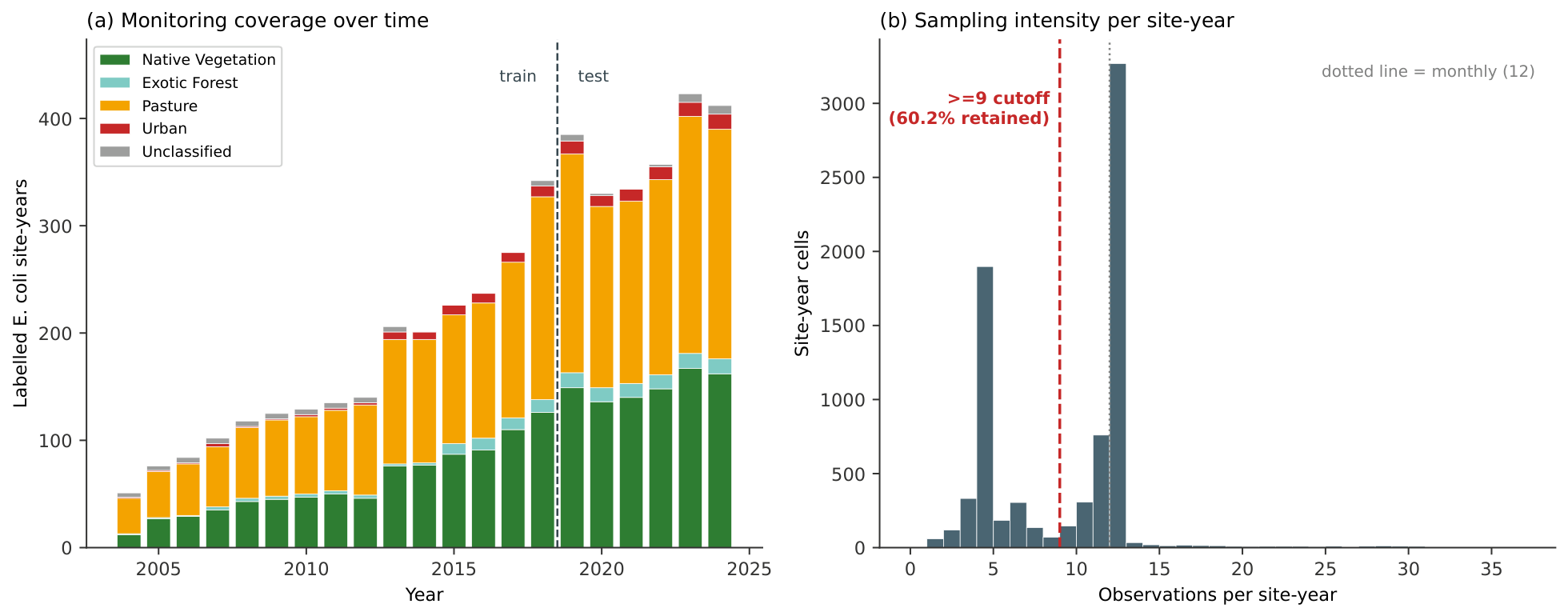
The spatial distribution of the 497 sites is shown in Figure 1. The study uses river water quality monitoring data for the South Island of New Zealand, obtained from the Land, Air, Water Aotearoa (LAWA) national monitoring database [16]. The South Island spans a strong land-use gradient, from near-pristine native vegetation catchments in the mountainous interior and west to intensively farmed pastoral lowlands and growing urban centres in Canterbury, Marlborough, Nelson, Tasman, Otago, Southland, and the West Coast. This gradient makes the region well suited to a cross-site analysis of how catchment character relates to compliance risk (Figure 2a).
The extract analysed here covers approximately two decades of monitoring (2004–2024) across 497 monitoring sites, comprising 680,231 individual measurements after cleaning. Sites are sampled at a typically monthly frequency under regional council state-of-the-environment programmes, and each record carries a site identifier, sampling date, indicator, measured value, a quality-control code, and catchment descriptors (land cover, latitude, and longitude). Eleven water quality indicators are retained as model inputs: E. coli, nitrate nitrogen, ammoniacal nitrogen, dissolved reactive phosphorus, total phosphorus, total nitrogen, turbidity, water clarity (black disc), dissolved inorganic nitrogen, total oxidised nitrogen, and pH. Summary statistics for the annual medians of all eleven indicators are given in Table A2.

2.1.1. Cleaning and Quality Control

Raw records were quality-screened against the National Environmental Monitoring Standards (NEMS) for discrete river water quality [24], under which each measurement may be assigned a quality code; in this extract, these ranged from QC 600 (highest quality) down to QC 200 (unverified). Measurements coded QC 200 (unverified) were discarded; all higher-quality codes (QC 300 and above) were retained. Records with missing values were dropped, sampling dates were parsed to a calendar year, and each remaining observation was assigned to a site–indicator–year cell. Sampling intensity is bimodal across site-years, reflecting quarterly and monthly monitoring regimes (Figure 2b). The ≥9-observation filter retains 60.2% of cells, deliberately excluding quarterly sampled cells so that each annual median, 95th percentile, and maximum is computed from enough observations to be representative; this trades network coverage for per-cell statistical reliability.
The large majority of records in this extract—over four-fifths—carry no NEMS code, reflecting inconsistent population of quality codes across regional councils rather than poor data quality. Two considerations support retaining these uncoded records. First, exclusion is infeasible: only a small fraction of records, and fewer than one in seven E. coli site-years, carry the highest QC 600 code, so restricting to fully coded data would discard most of the dataset and leave too few observations per site-year to compute robust annual statistics. Second, the resulting breach labels follow a strong, mechanistically expected land-cover gradient (Section 2.2); random measurement error in uncoded records would not produce this ordered structure, indicating that the breach signal reflects genuine water-quality variation rather than data-quality artefacts. The fully coded QC 600 subset covers 226 of the 497 sites and retains only 14.1% of E. coli site-years under the ≥9-observation requirement, too few to serve as a like-for-like validation sample; its land-cover composition, however, is close to that of the full network (Appendix B.3). Absolute breach rates are therefore interpreted as network-level estimates from operational monitoring data. Uncoded records were retained and processed identically to coded records.
To ensure annual statistics were representative rather than driven by sparse sampling, only site–indicator–year cells with at least nine observations were used. For each retained cell, the annual median was taken as the central summary, with the 95th percentile and annual maximum additionally computed for the compliance-labelling rules described in Section 2.2.

2.1.2. Catchment Land Cover

Each site was assigned a dominant catchment land-cover class from the RECLandCover field supplied in the LAWA dataset. These classes are derived from the New Zealand River Environment Classification (REC) [25] and grouped, following LAWA’s national river water quality reporting [26], into four dominant-cover classes: native vegetation, exotic forest, pasture, and urban (with sites lacking an assignment retained as “unclassified”). It is important to note that these are dominant -cover classes rather than pure ones: a native vegetation catchment is one in which native cover predominates upstream and may still contain minor pasture, exotic forest, or urban areas, consistent with the mixed-catchment categorisation rules of the REC land-cover scheme [27]. The distribution of sites across the four classes is summarised in Table 1.
The network is dominated by pastoral (53.1%) and native vegetation (36.4%) catchments; urban and exotic forest sites are comparatively few (16 and 14 sites, respectively), which limits the precision of within-class estimates for those two classes (Section 3).

2.2. Compliance Labelling

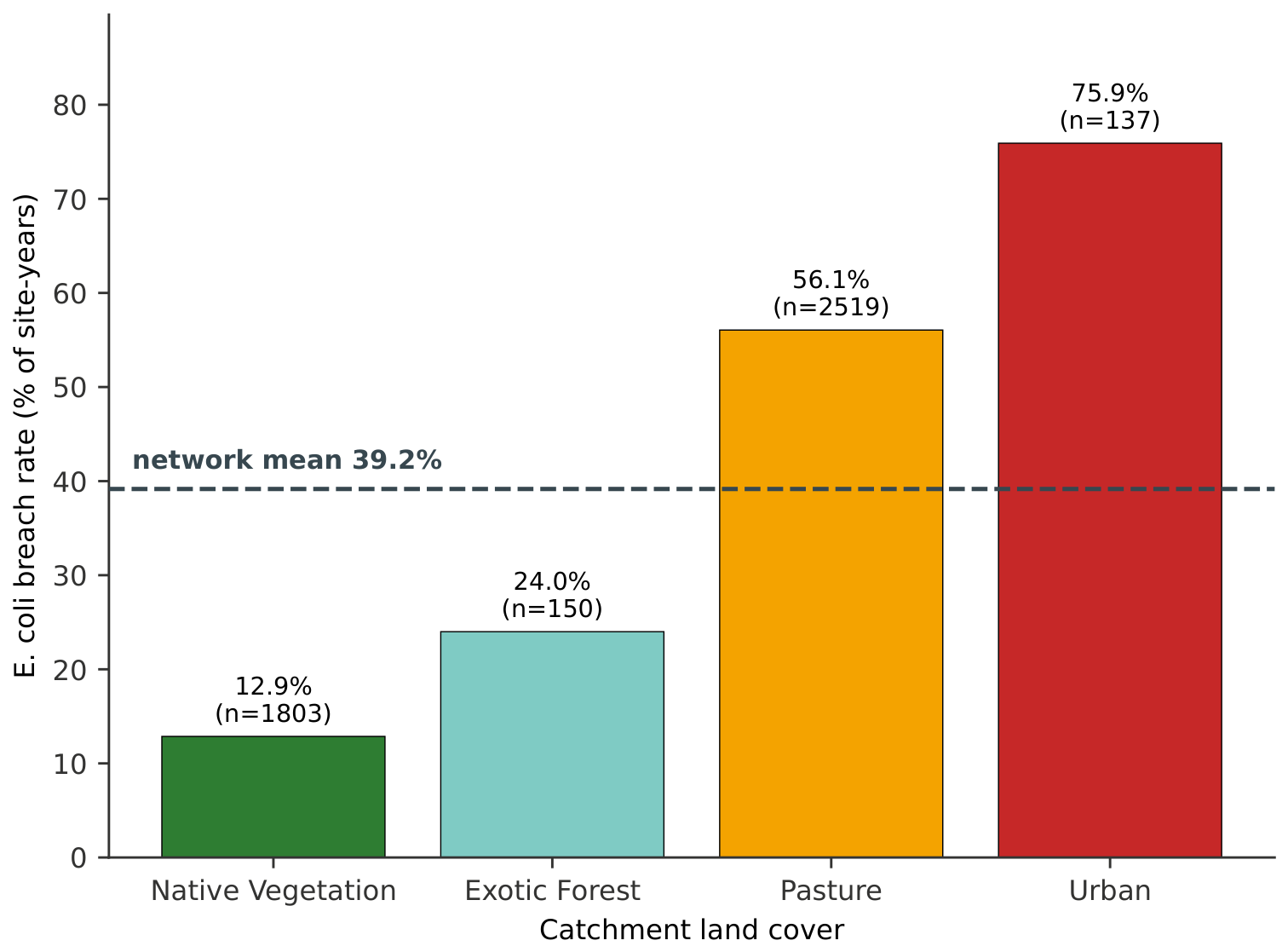
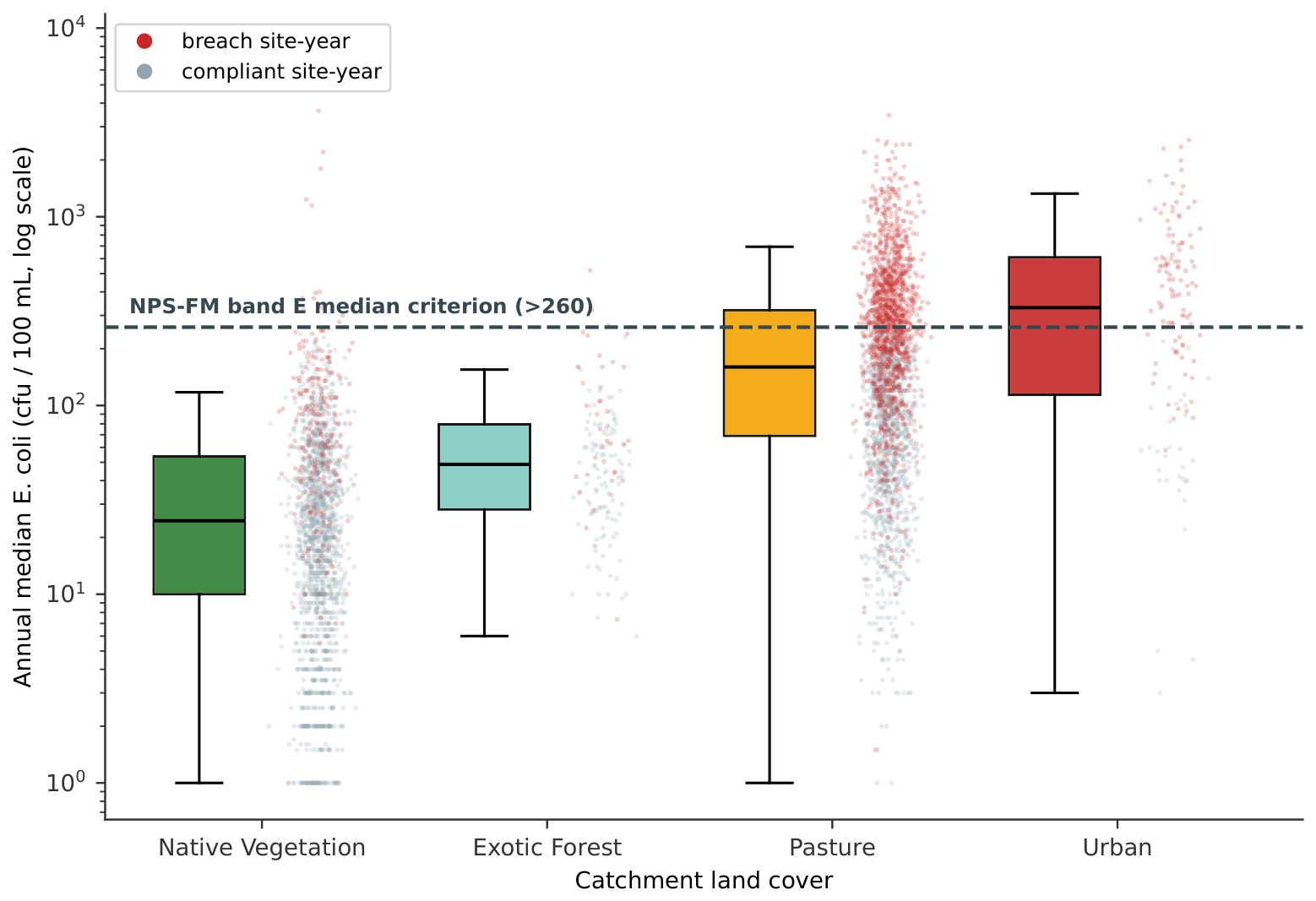
The forecasting target is annual compliance with the National Policy Statement for Freshwater Management 2020 (NPS-FM) [23]. The NPS-FM grades each attribute from Band A (best) to Band D or E (worst) and, for a subset of attributes, defines a national bottom line—a legally enforceable minimum below which a site is required to improve. Breach prevalence followed a clear land-cover gradient (Figure 3), rising monotonically from native vegetation through pasture to urban catchments.
We define the binary compliance-breach target on E. coli alone, because it is the human-contact attribute for which the NPS-FM specifies a national bottom line and which therefore carries an unambiguous regulatory meaning for a “breach” [23]. A site-year is labelled non-compliant (breach) when it falls into the worst attribute band (Band E) for E. coli—the most degraded NPS-FM state, which lies below the national bottom line defined as satisfying any of the four statistical criteria in Table 2. Dissolved reactive phosphorus (DRP) is an ecosystem-health attribute with no national bottom line; it is therefore not treated as a compliance-breach target and is instead reported separately as a descriptive action-planning indicator (Section 2.7).
The underlying concentration gradient driving these breach rates is shown in Figure 4; note that some breaching site-years fall below the median line, reflecting breaches triggered by the 95th-percentile or exceedance criteria.
Applying this rule yielded 4688 site-years with a valid E. coli label, of which 39.2% were breaches. Breach prevalence followed a clear land-cover gradient, rising monotonically from 12.9% at native vegetation sites through 24.0% (exotic forest) and 56.1% (pasture) to 75.9% at urban sites.

2.3. Feature Construction

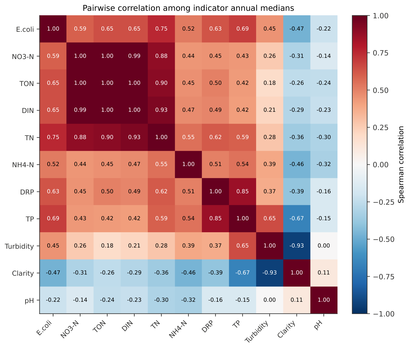
The eleven indicators are substantially inter-correlated (Figure 5), particularly within the nitrogen species, which informs the per-indicator aggregation of SHAP contributions in the interpretation of forecast drivers. The forecasting problem is framed as a supervised, cross-site binary classification task: using information available up to a given origin year, predict whether a site will breach the E. coli national bottom line h years into the future, for horizons h { 1 , 2 , 3 } . Pooling all sites into a single model rather than fitting one model per site allows the classifier to learn land-cover and catchment signatures that transfer across the network, including to sites with short individual records.
For every site and year, the annual median of each of the eleven indicators was arranged into a site-by-year feature matrix. From this matrix, three families of predictors were derived for each indicator:
  • Lagged levels: the annual median at the origin year and at each of the three preceding years of record (lags 0–3), capturing recent absolute conditions.
  • Three-year trend: the change in annual median over the three preceding years of record, capturing the local direction of travel.
  • Current breach status: a binary flag for whether the site is in breach at the origin year, which both anchors the model and defines the persistence baseline (Section 2.5).
The three-year lookback is bounded by data availability rather than chosen on statistical grounds. Lag-3, together with the three-year trend, requires four consecutive qualifying years of record at a site, which, under the ≥9-observation filter (Section 2.1.1), is already restrictive; a longer window would reduce the rows available for training without a corresponding gain in information. The resulting four-year span from the origin year also sits close in scale to the five-year window LAWA uses for its own attribute-state assessment. These were combined with four static catchment descriptors.
These were combined with four static catchment descriptors—land cover, region, latitude, and longitude—giving 60 predictors in total (Table 3). Land cover and region were passed to the model as native categorical features. The prediction target y for a row at origin year t is the E. coli breach label at year t + h ; rows were formed by an inner join between the feature matrix at t and the label at t + h , retaining only rows with a defined current breach status.

2.4. Forecasting Model

Forecasts were produced with a gradient-boosted decision tree classifier (LightGBM) [28], chosen for its strong performance on tabular data with mixed numerical and categorical features, its native handling of categorical variables, and its robustness to the correlated, partially missing predictors typical of multi-indicator monitoring records. A single model was trained per horizon. Hyperparameters were held fixed across horizons (400 boosting rounds, learning rate 0.03, 31 leaves, and 0.8 row and column subsampling), and a fixed random seed was used for reproducibility. Rather than reweighting classes to address the imbalance between compliant and non-compliant site-years, the decision threshold was tuned explicitly (Section 2.5), which keeps the predicted probabilities on their natural scale for the calibration analysis in Section 2.6.

2.5. Baselines and Temporal Validation

Because compliance status is highly persistent year to year, a forecast model is only useful if it improves on simply assuming next year looks like this year. The model was therefore benchmarked against three baselines:
  • Persistence: predict the future label to equal the current breach status. This is the primary benchmark to beat, and—by construction—it cannot flag any site that changes status.
  • Trend projection: linearly extrapolate the current indicator value by its recent per-year slope and compare the projection to the threshold.
  • Majority class: predict no breach for all site-years.
Validation used a strictly temporal hold-out to avoid any leakage of future information: models were trained on origin years whose target year fell on or before 2018 and evaluated on target years from 2019 to 2024. The operating threshold was selected on the two most recent training origin years (an internal validation slice, never the test set) by maximising balanced accuracy, and a single fixed threshold was then applied across all three horizons so that year-on-year forecast counts remain comparable.
Two further checks established that the model’s edge over persistence is genuine rather than an artefact of one particular split. First, a rolling-origin analysis repeated the temporal hold-out across successive origin years (2015–2018), confirming the direction and stability of the gain. Second, a paired bootstrap (2000 resamples of the test set) produced 95% confidence intervals on balanced accuracy and on the model-minus-persistence gap; the gap was treated as a real improvement only where its interval excluded zero.
Aggregate accuracy is dominated by the large number of sites whose status does not change, where persistence is already correct. The operationally meaningful question is narrower: among sites that are currently compliant, how many of those that go on to breach can the model flag in advance? This early-warning evaluation restricts the hold-out to currently passing site-years and reports precision and recall on the subset that subsequently enters the worst band (Band E). Persistence scores zero recall on this subset by construction, making it the natural reference against which the model’s forward-looking value is measured.

2.6. Calibration and Feature Attribution

For a risk forecast to support prioritisation, its scores should rank sites reliably; for them to be read as literal breach probabilities, they should also be calibrated. Calibration was assessed on the temporal hold-out using the Brier score (against a predict-the-base-rate reference) and decile reliability curves of predicted versus observed breach frequency. Where the raw scores were over-confident, post hoc recalibration was examined using both isotonic regression and Platt (sigmoid) scaling, fitted out-of-time so that any improvement would have to hold on genuinely future data rather than in-sample. The reporting decision that follows from this analysis is given in Section 3.
Finally, model behaviour was interpreted with SHAP (SHapley Additive exPlanations) values [29], with per-indicator contributions summed across lags to identify which monitoring signals drive the forecasts, and performance was additionally broken down within each land-cover class to check that skill is not confined to a single catchment type.

2.7. Dissolved Reactive Phosphorus as an Action-Planning Indicator

DRP is reported alongside the E. coli forecast but is treated distinctly. As an Appendix B.2 ecosystem-health attribute, DRP has no NPS-FM national bottom line, so its exceedances cannot be interpreted as regulatory breaches. DRP worst-band exceedance was modelled with the same feature set and horizons, and its scores are presented as a descriptive, catchment-prioritisation signal rather than a compliance forecast. The distinction is made explicit so that DRP risk informs action planning without being conflated with enforceable non-compliance.

3. Results

Results are reported on the strictly temporal hold-out described in Section 2.5: models are trained on origin years whose target falls on or before 2018 and evaluated on target years 2019–2024, for horizons h { 1 , 2 , 3 } . Throughout, E. coli non-compliance is the sole breach target and persistence—next year equals this year is the primary benchmark, because it is both the operationally obvious heuristic and the one a useful forecast must beat. The operating threshold was selected on the two most recent training origin years (an internal validation slice, never the test set) by maximising balanced accuracy, and a single fixed threshold was then applied across all three horizons so that year-on-year forecast counts remain comparable.

3.1. Forecast Skill Relative to Baselines

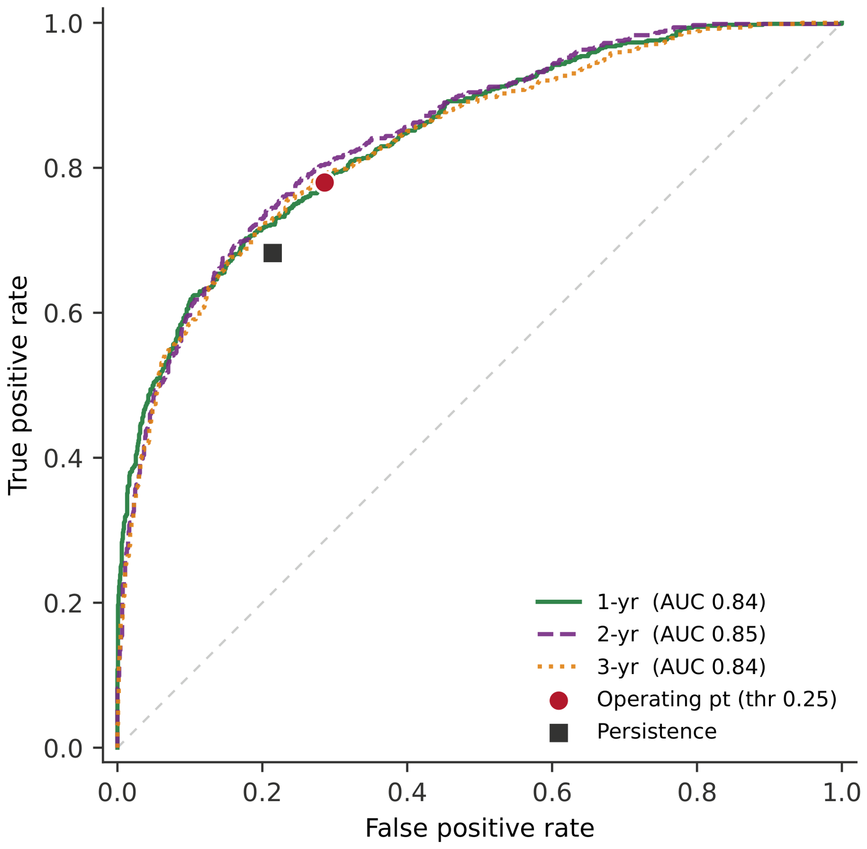
Discrimination is strong and stable across horizons, with area under the ROC curve of 0.844, 0.847, and 0.836 at the one-, two-, and three-year horizons (Table 4, Figure 6); the one-year estimate carries a bootstrap 95% interval of [0.825, 0.861], well clear of the 0.5 no-skill line. The practical consequence is clearest at persistence’s own operating point: holding the false positive rate equal to persistence (about 0.21), the model raises the true positive rate from 0.66–0.68 to 0.72–0.75 at every horizon—the same volume of false alarms but appreciably more breaches caught. (Table 4, Figure 6); the one-year estimate carries a bootstrap 95% interval of [0.835, 0.869], well clear of the 0.5 no-skill line. The practical consequence is clearest at persistence’s own operating point: holding the false positive rate equal to persistence (about 0.21), the model raises the true positive rate from 0.66–0.69 to 0.74 at every horizon—the same volume of false alarms but appreciably more breaches caught.
At the fixed 0.25 operating point, the model improves on persistence in balanced accuracy at all three horizons: 0.747 against 0.734 at one year, 0.765 against 0.731 at two years, and 0.755 against 0.719 at three years, with trend projection reaching 0.690 and the majority class 0.500. A paired bootstrap (2000 resamples, evaluated at the same fixed threshold) gives 95% confidence intervals for the model-minus-persistence difference of [ 0.008 , + 0.033 ] , [ + 0.011 , + 0.056 ] , and [ + 0.011 , + 0.060 ] . The two- and three-year gaps exclude zero; the one-year interval does not, and the aggregate one-year advantage is therefore not statistically distinguishable from persistence at this threshold. Threshold-free discrimination at one year is nevertheless well established (AUC 0.844, 95% CI [0.825, 0.861]), and the operationally decisive comparison is not aggregate accuracy but recall on status transitions (Section 3.3), where persistence scores zero by construction, and the margin is therefore unbounded rather than marginal. A rolling-origin analysis over successive origin years (2015–2018) reproduced the advantage in every split, with per-split balanced-accuracy gaps of + 0.033 (2015), + 0.029 (2016), + 0.041 (2017), and + 0.013 (2018) and AUC between 0.844 and 0.859. The gain is positive at every boundary tested, though smallest at the 2018 split reported above, indicating that the headline comparison is drawn from the least favourable of the four rather than a selectively advantageous one.
At the 0.25 operating point, the model recovers the large majority of breaches while holding false alarms to roughly a quarter of compliant site-years: precision ranges from 0.60 to 0.62, recall from 0.77 to 0.78, and the proportion of compliant site-years flagged from 0.25 to 0.29 across the three horizons (Table 4). In ROC space, the operating point sits well above the persistence point at a comparable false positive rate (Figure 6), confirming the gain is a genuine shift in the recall–false-alarm trade-off rather than a relabelling of the same decisions.
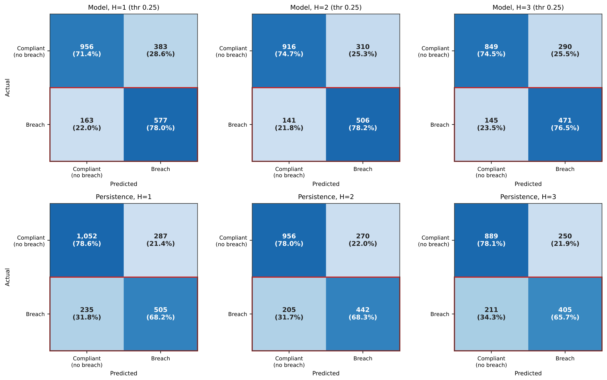
The recall–false-alarm trade-off underlying these balanced-accuracy figures is shown in Figure 7: the model recovers 577 of 740 hold-out breaches against persistence’s 505, while raising more false alarms among compliant site-years.

3.2. Operating Threshold and Decision Analysis

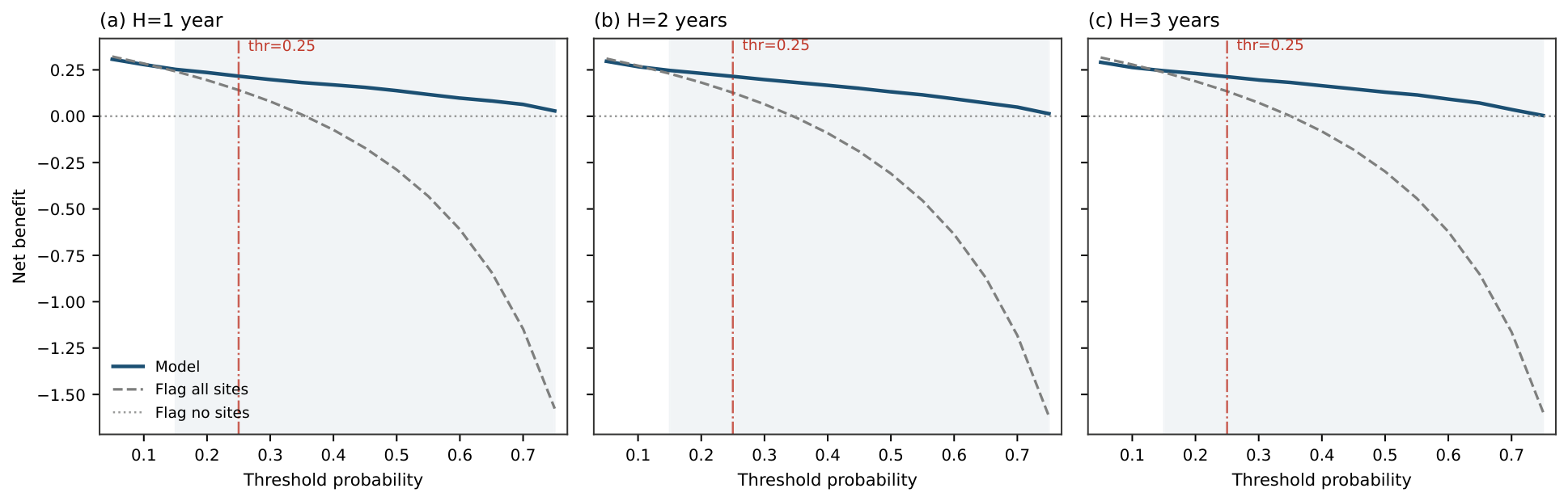
The 0.25 operating point reflects a recall-oriented screening posture rather than an optimum. Because the appropriate balance between missed breaches and unnecessary inspections depends on a council’s investigative capacity, we report performance across the full range of operating thresholds and evaluate the forecast under a decision-analytic framework in which the threshold probability p t also encodes the assumed cost of a false positive relative to a false negative, with weight w = p t / ( 1 p t ) . Net benefit (NB) is then TP / n ( FP / n ) × w , computed for the forecast and for the two policy alternatives available without a model: inspect every site and inspect none.
Two distinct quantities are separated throughout. The false alarm rate is the proportion of compliant site-years that are flagged (the false positive rate reported in Section 3.1), whereas the false alert rate is the proportion of issued alerts that do not eventuate in a breach ( 1 precision ). At the 0.25 operating point, the false alert rate is 39.9%, 38.0%, and 38.1% at the one-, two-, and three-year horizons, respectively: a minority of alerts, not a majority.
The comparison in Table 5 is between the three net-benefit columns within each row, since all three share the cost weight implied by that row’s threshold; values in different rows are computed under different cost assumptions and are not directly comparable. On that basis, the forecast yields higher net benefit than both inspecting every site and inspecting none at every threshold from 0.15 to 0.75 and at all three horizons (Figure 8). Below 0.15, the implied cost of a false positive becomes low enough that indiscriminate inspection is marginally competitive, which is of little practical interest given finite monitoring budgets.
The threshold therefore selects an operating position rather than a level of forecast skill. Raising it from 0.25 to 0.50 at the one-year horizon reduces the flagged set from 960 to 715 site-years and recall from 0.78 to 0.68—roughly a quarter fewer inspections for approximately ten percentage points of additional missed breaches. A council can enter Table 5 at its own inspection capacity and read off both the corresponding threshold and the recall it can expect, which is the intended operational use of the forecast.

3.3. Early Warning of Emerging Breaches

Aggregate accuracy is dominated by many sites whose status does not change, where persistence is already correct, and so understates the forecast’s practical value. The operationally decisive question here is to determine, among sites that are currently compliant, how many of those that subsequently enter the worst band (Band E) can the model flag in advance. Restricting the hold-out to currently passing site-years isolates exactly the transitions that persistence cannot, by construction, ever detect.
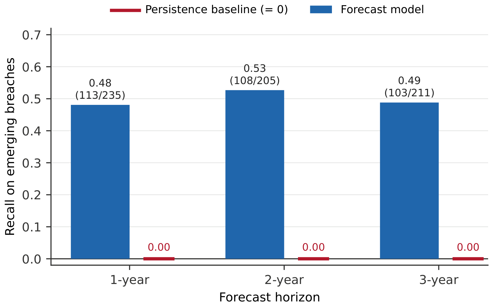
On this subset, the model identifies roughly half of all emerging breaches at every horizon: 113 of 235 transitions at one year (recall 0.48), 108 of 205 at two years (0.53), and 103 of 211 at three years (0.49) (Table 6, Figure 9). The cost of that early warning must be stated in the same breath. Recall is achieved at modest precision (0.37–0.40) because the model also raises 195, 164, and 163 false alarms among the 1052, 956, and 889 stable compliant sites at the three horizons. The tool is therefore best understood as a recall-oriented screening instrument for prioritising investigative monitoring, not as a high-precision predictor of individual site failure; acting on its watchlist means accepting that a minority of flagged sites will not, in the event, breach.
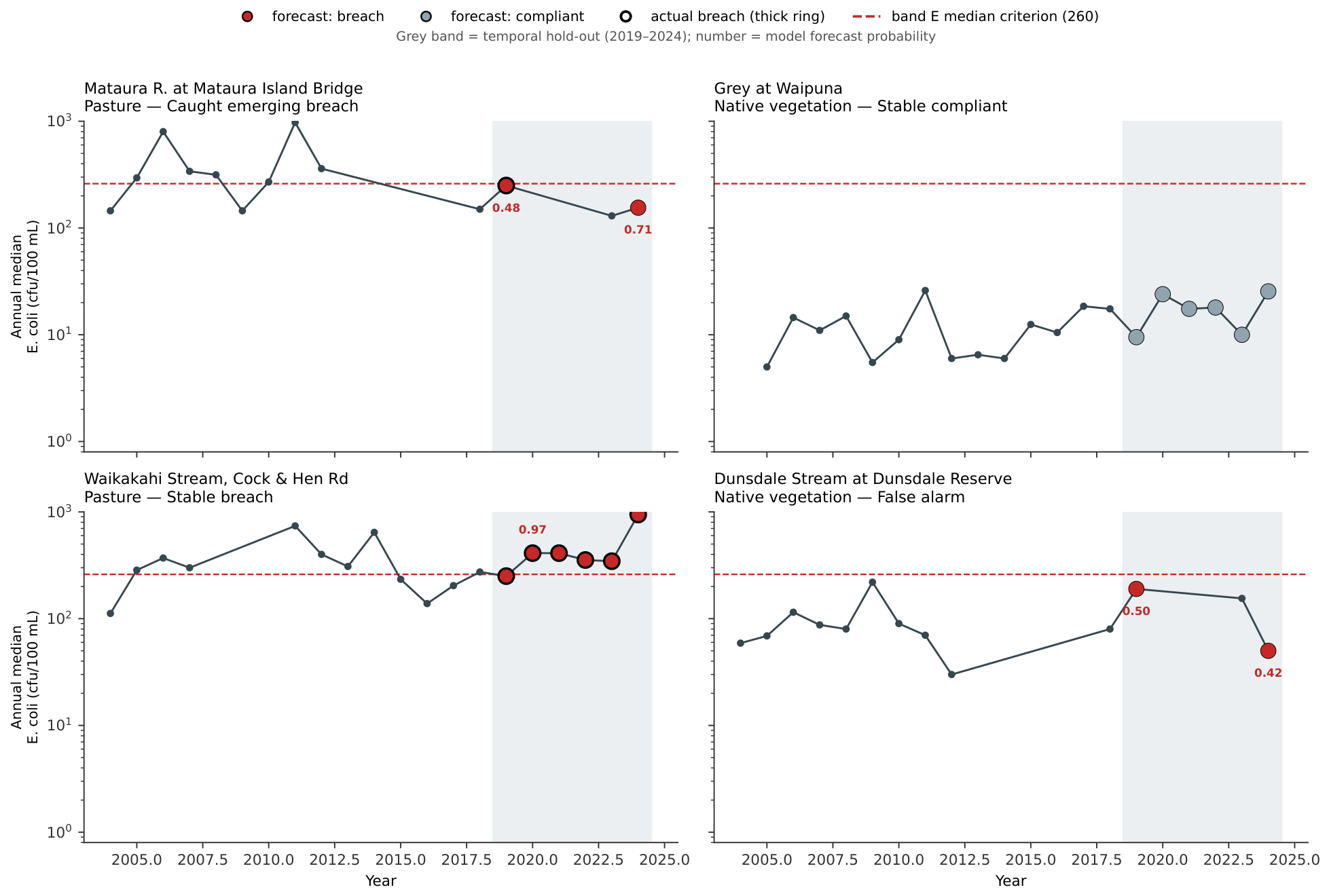
Figure 10 illustrates these dynamics at four representative sites: the model issues an early warning at a site approaching the worst band (Mataura), correctly holds a clean native vegetation site compliant (Taieri), tracks a persistent breach with high confidence (Waikakahi), and demonstrating the precision cost raises a false alarm at a compliant native vegetation site (Dunsdale).

3.4. Calibration and Score Reporting

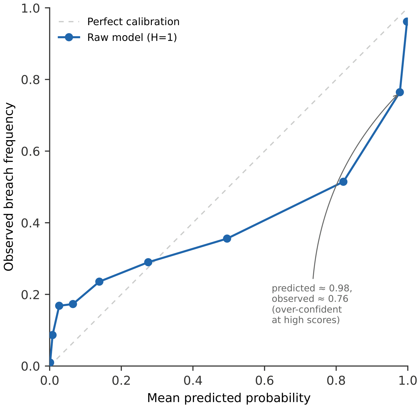
For the forecast scores to be read as literal breach probabilities, they must be calibrated, not merely well ranked. On the hold-out, the raw model scores attain a Brier score of 0.167 (against 0.229 for a predict-the-base-rate reference), compared with 0.209 for full-history Platt (sigmoid) scaling and 0.190 for a sigmoid fitted on the most recent training years. Platt scaling therefore degrades the raw scores under both fitting regimes. Isotonic regression, fitted out-of-time on a reduced calibration split, marginally improves on the raw scores evaluated on that same split (0.152 against 0.159), but the improvement is small and rests on a smaller fitting sample than the Platt comparisons, so it does not establish that recalibration transfers reliably in future data. Reliability curves show the raw scores are well calibrated at the low end but increasingly over-confident from the middle of the score range upward, with the highest decile predicting 0.98 against an observed breach rate of 0.76, where predicted breach rates run ahead of observed frequencies (Figure 11), where predicted breach rates run ahead of observed frequencies (Figure 11). Reliability curves show the raw scores are well calibrated at the extremes but somewhat over-confident through the upper-middle of the score range, where predicted breach rates run ahead of observed frequencies (Figure 11).
The reporting decision follows directly because no recalibration yields a reliable out-of-time improvement, and because the operational use of the scores is to order sites rather than to state probabilities, the model outputs are reported as risk rankings rather than calibrated probabilities, accompanied by an explicit statement of this drift limitation. Scores are used to order sites for prioritisation and to apply the fixed operating threshold; they are not interpreted as exact probabilities of breach.

3.5. Forecast Drivers and Within-Catchment Performance

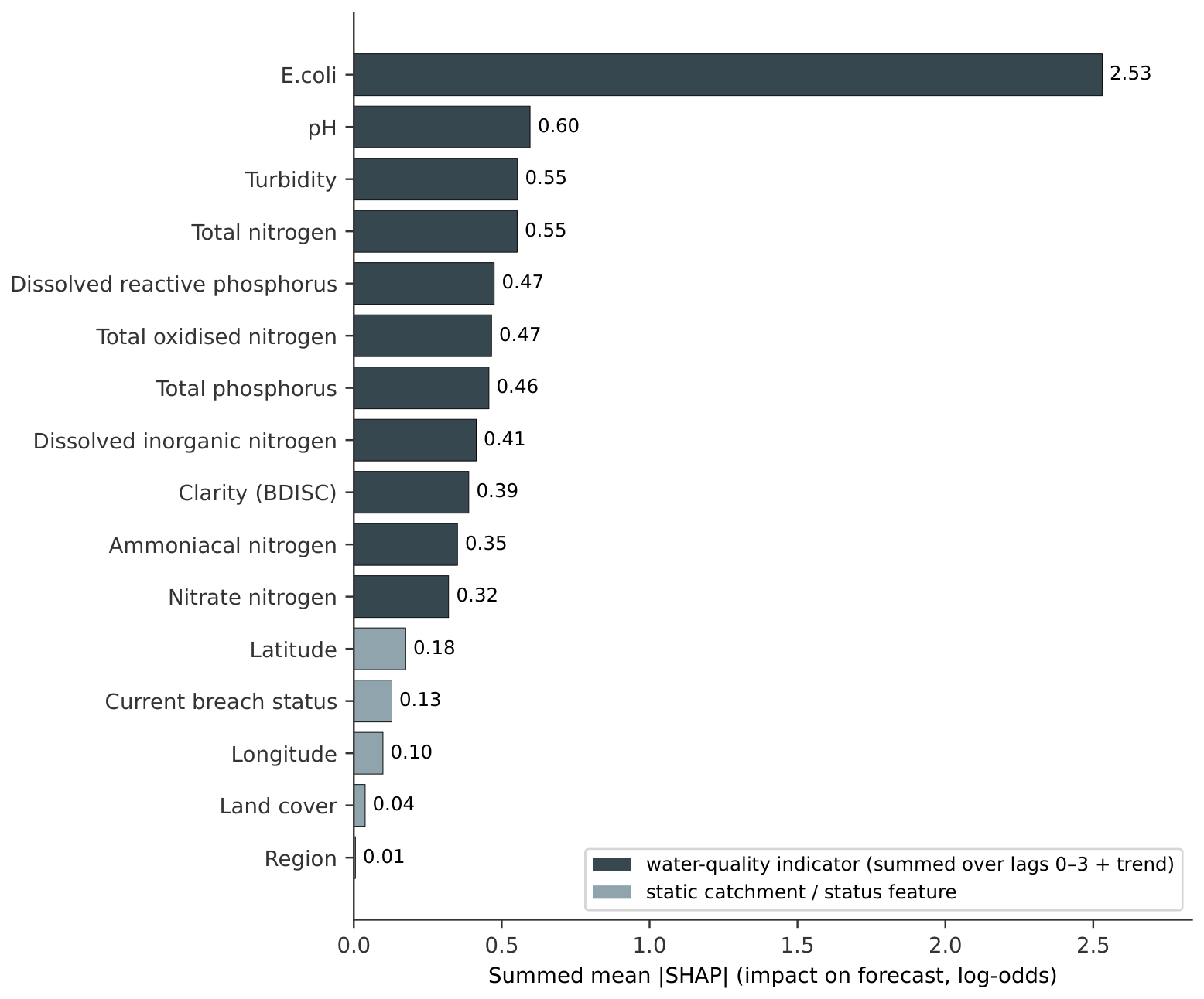
SHAP attribution, with per-indicator contributions summed across lags, shows the forecasts are driven overwhelmingly by a site’s own recent E. coli history (summed mean |SHAP| of 2.53, far above any other input), followed at a distance by pH (0.60) and turbidity (0.55), then total nitrogen and dissolved reactive phosphorus. The binary current-breach flag contributes little (0.13), indicating that the model draws its signal from the continuous trajectory of recent water-quality measurements rather than from current compliance status alone—which is what allows it to anticipate transitions that a status-copying rule cannot.
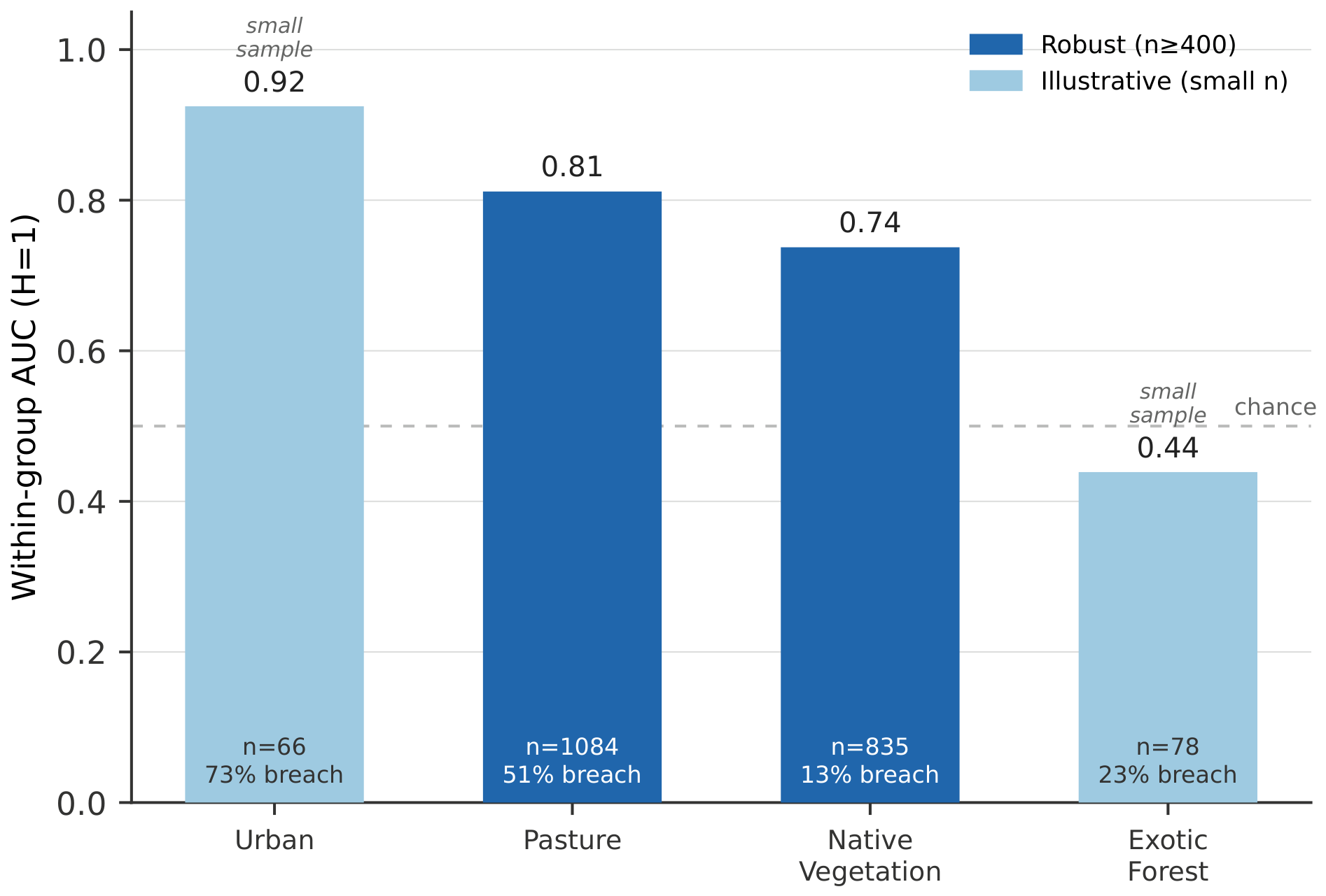
This is not confined to a single catchment type. Within-class AUC at the one-year horizon is 0.74 for native vegetation and 0.81 for pasture sites—the two classes with sufficient site-years to support a like-for-like estimate (Figure 12). The urban (AUC 0.92, 66 test site-years) and exotic forest (0.44, 78 site-years) estimates are reported for completeness but rest on too few observations for confident interpretation; the sub-chance exotic forest value in particular reflects small-sample noise rather than a genuine absence of characteristic. The breach base rate itself follows the expected land-use-intensity gradient, rising from 12.9% at native vegetation sites through 24.0% (exotic forest) and 56.1% (pasture) to 75.9% at urban sites; that the model retains discrimination within the higher-loading classes, where most breaches occur, is what makes the forecast operationally useful rather than a restatement of land cover. One year feature attribution forecast for all the features are shown in Figure 13.

3.6. Contribution of the Multi-Indicator Feature Set

Feature attribution (Section 3.5) shows the forecast is dominated by a site’s own recent E. coli history, raising the question of whether the remaining ten indicators contribute materially. To test this directly, the model was refitted using only six predictors—E. coli at lags 0–3, the E. coli three-year trend, and dominant catchment land cover—and compared with the full 60-predictor model on the same temporal hold-out, split, and operating threshold.
On threshold-free discrimination the two are close to indistinguishable: the full model attains AUC advantages of 0.001, 0.011, and 0.010 at the one-, two-, and three-year horizons. Recent E. coli history therefore carries most of the discriminative signal, consistent with the attribution results.
Comparison on early-warning performance requires care, because the two models place different proportions of the score distribution above a given probability. At the common 0.25 threshold, the reduced model appears to recover more transitions (140 against 113 at one year), but it does so by flagging substantially more currently compliant sites: 256 false alarms against 195, a false positive rate of 0.243 against 0.185. The apparent advantage reflects a more permissive operating point rather than superior early-warning skill.
Table 7 reports the comparison at matched operating points. Holding the false positive rate among stable compliant sites equal to that of the full model, the full model recovers more transitions at two of the three horizons, with the margin largest at two years (108 against 90); matching instead on the total number of flagged sites reproduces the same pattern. At one year, the reduced model retains a modest advantage under both matching schemes. This is consistent with balanced accuracy, on which the full model leads at every horizon (Table 4).
The multi-indicator design does not provide a large improvement in overall discrimination. Its main benefits are different. First, it provides early-warning performance that is at least comparable to a single-indicator model. It also performs no worse when both models are compared at the same operating point. Second, it allows us to identify which indicator is driving the increased risk. This helps explain why a site has been flagged. For a screening tool, this information is important. It is not enough to know that risk has increased. It is also useful to know which water-quality indicator is changing. This can help guide further monitoring and investigation.

3.7. Transferability Across Regions

Pooling all sites into a single model rests on the premise that catchment signatures learned in one part of the network transfer to another (Section 2.3). To test this directly, the model was refitted seven times, each time excluding one region’s site-years from training entirely, and evaluated on that held-out region. A model that had merely memorised region-specific behaviour would degrade sharply when denied its own region’s training data.
At the one-year horizon, the difference between the full-network model and the region-excluded model ranges from 0.030 to + 0.036 AUC across the seven regions (Table 8), with three regions scoring marginally higher when their own data are withheld—a pattern consistent with sampling variation rather than systematic loss. The largest degradations occur at Southland ( 0.030 ) and Tasman ( 0.022 ), both of which retain AUC above 0.81. Discrimination in the two largest regions, Canterbury and Otago, is essentially unchanged.
The same procedure applied to the DRP model gives differences between 0.010 and + 0.025 at six of seven regions, with one exception: West Coast falls by 0.051, from 0.979 to 0.928. Given the low DRP worst-band prevalence there (0.135 of 193 site-years), this is most plausibly a small-sample effect, but it is reported rather than omitted. The result supports the pooled cross-site design and, by extension, the model’s applicability to sites whose own records are too short to support site-specific fitting.

3.8. Forward Forecast, 2025–2027

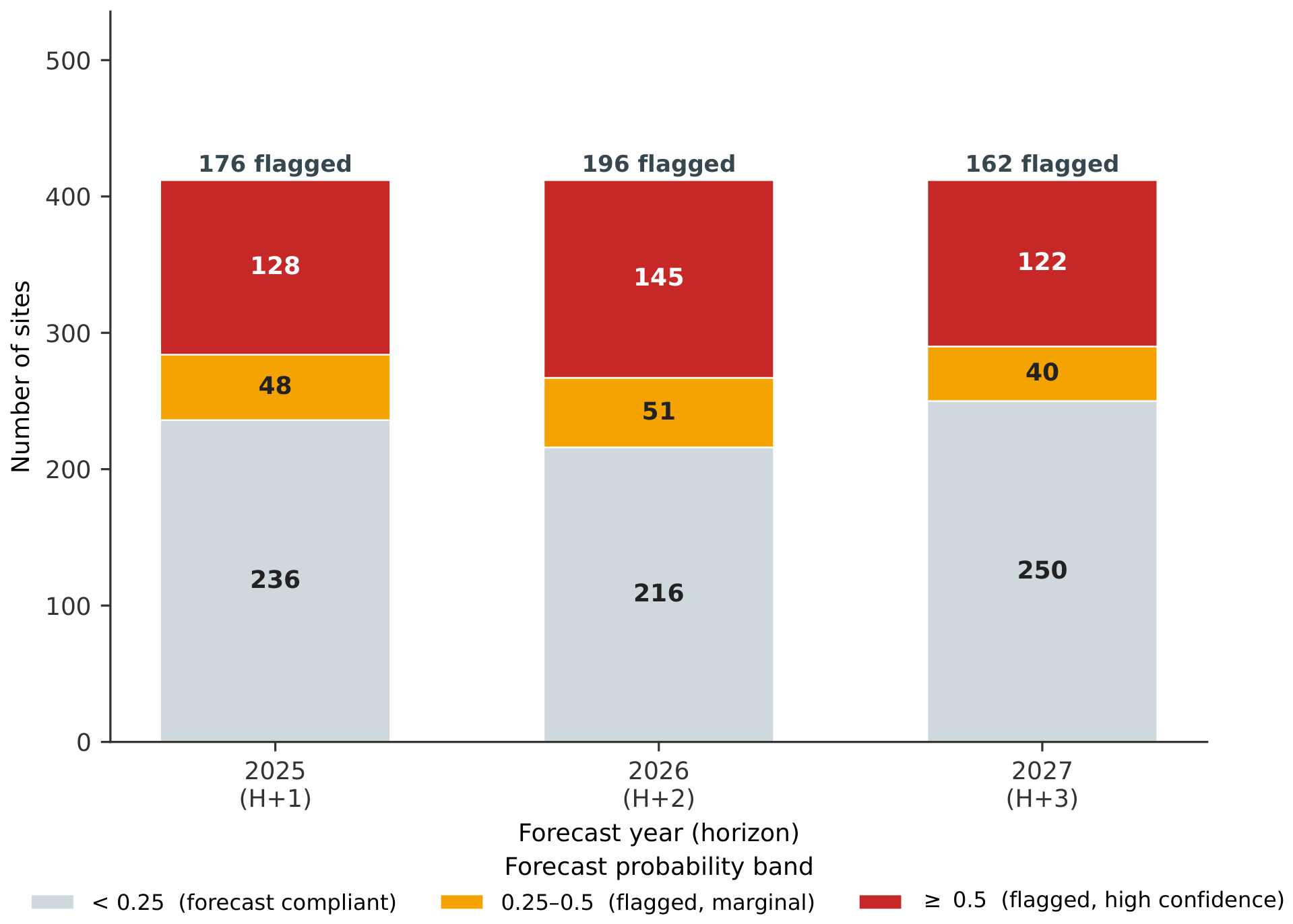
For the operational forecast, the model was refit on all labelled data and applied from a 2024 origin to project E. coli compliance for 2025–2027. This forward step is reported separately from the frozen hold-out evaluation above: it uses every available year of labels to maximise currency, at the cost of having no future labels against which to score it directly. Forecasts were produced for the 412 sites carrying a valid 2024 origin record (Figure 14).
The model projects 176, 196, and 162 sites in breach in 2025, 2026, and 2027, respectively. This modest decline across horizons should not be read as projected improvement in water quality. The subset of sites scored with high confidence (probability at or above 0.5) is essentially stable across horizons (128, 145, and 122 sites), while the median forecast probability is 0.194, 0.212, and 0.129 at the one-, two-, and three-year horizons, broadly flat before falling at the longest horizon. The attenuation therefore occurs among marginal cases, which slip back below the operating threshold as the forecast extends further from the last observed data, the expected behaviour of a forecast built on monitoring records alone, without the dynamic hydroclimatic drivers that govern shorter-term E. coli variability.
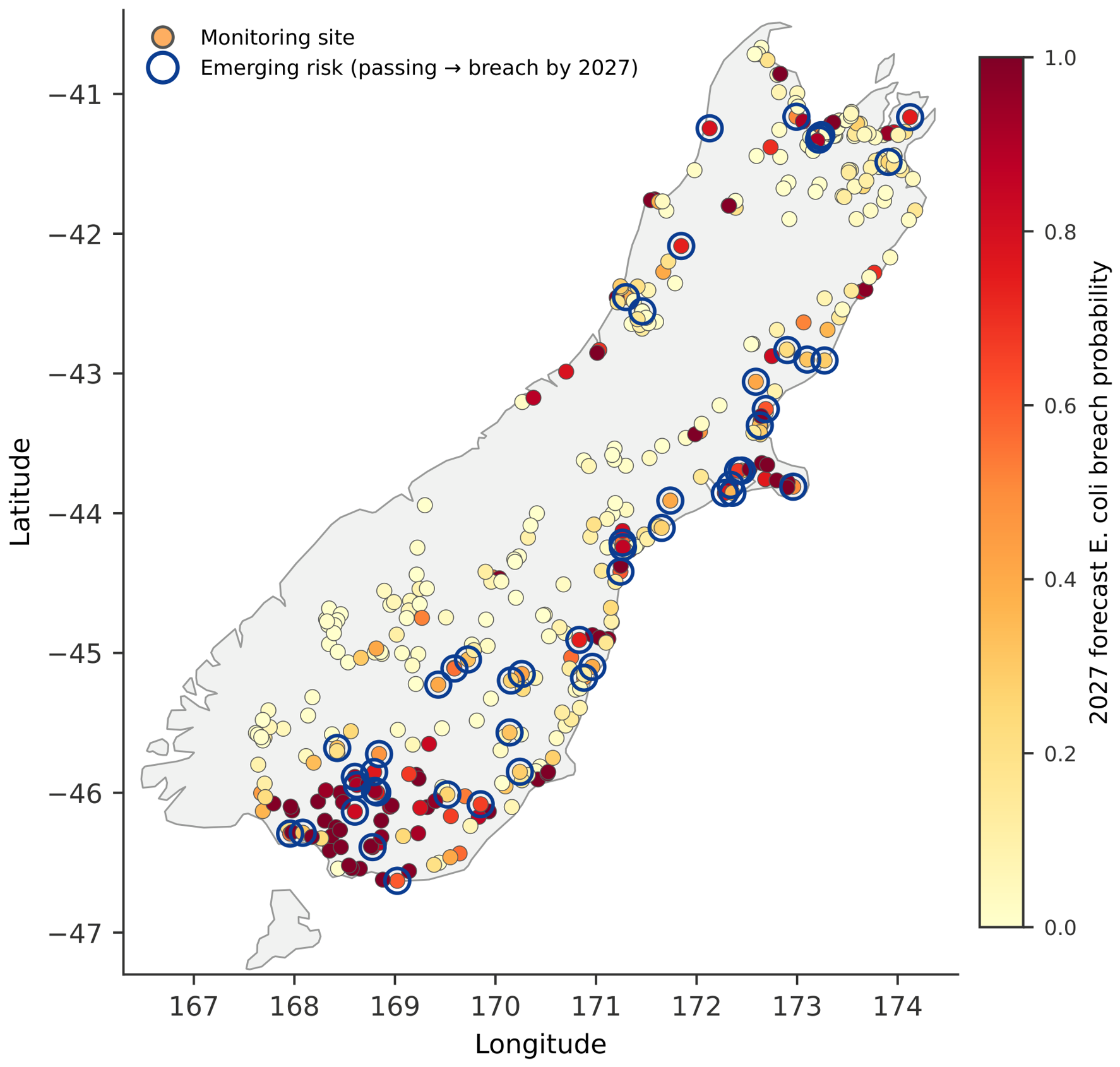
The key output is the emerging-risk watchlist: sites currently compliant that are forecast to breach. The model flags 60 such sites for 2025, 79 for 2026, and 51 for 2027, and 97 distinct currently compliant sites are flagged in at least one of the three years. These emerging-risk sites are concentrated in pastoral catchments (69 of the 97), with native vegetation sites (20), mirroring the breach gradient and the predominance of pasture in the network. Figure 15 maps the 2027 forecast across the South Island and rings the 51 sites forecast to degrade from compliant to breaching by that year, locating the emerging risk geographically for monitoring prioritisation.

3.9. Dissolved Reactive Phosphorus as an Action-Planning Signal

DRP worst-band status is highly stable year to year, which makes it easy to rank (model AUC 0.95–0.97) but leaves little forecasting headroom over persistence: evaluated at the common 0.25 operating point, persistence in fact attains higher balanced accuracy than the model at all three horizons (differences of 0.025 , 0.054 , and 0.063 , 95% intervals excluding zero). This reinforces the decision to treat DRP as a descriptive ranking for action planning rather than as a forecasting contribution in its own right. Of 411 sites with a valid origin, 52 were in the DRP worst band at the origin year, and the model projects 48, 52, and 49 sites in the worst band for 2025–2027, with 54 distinct sites flagged in at least one year. As with E. coli, the DRP signal is overwhelmingly pastoral (50 of the 54 flagged sites), reinforcing the land-use reading of nutrient as well as faecal-indicator risk. These DRP results are presented strictly to inform action planning and are not combined with the E. coli forecast or interpreted as regulatory non-compliance.

4. Discussion

This study sets out to test whether multi-year, regulatorily relevant compliance breaches can be forecast from sparse monthly monitoring records alone and whether such forecasts add value over the obvious heuristic that next year will resemble this one. Three key results are discussed here. First, a single pooled gradient-boosted model discriminates E. coli worst-band (Band E) breaches well and stable across all horizons (AUC 0.84–0.85). It also improves on persistence in balanced accuracy at every horizon, with bootstrap intervals that exclude zero at two and three years, though not at one. Second, and more importantly, the model recovers roughly half of the breaches that occur at sites that are currently compliant—the transitions that a persistence rule cannot, by construction, ever flag. Third, the raw model scores rank risk reliably but do not remain calibrated out-of-time, so they are most defensibly reported as risk rankings rather than as literal breach probabilities. Together, these results support the working hypothesis that operational monitoring data carry enough signal for genuine early warning, while also delineating, honestly, where that signal runs out.

4.1. Relationship to Prior Water-Quality Forecasting

Most machine learning work on river water quality applies a different approach from the one addressed here, which complicates direct comparison. A few of the studies did forecast composite water-quality indices at short horizons (hours to days) from high-frequency sensor streams using LSTM and hybrid convolutional–recurrent architectures. The classification accuracies in excess of 99% and R 2 values approaching unity have been reported for index prediction [5,7,8]. Those figures are not a benchmark this study can or should match, for two reasons. These studies describe interpolation of a smoothly varying signal over short intervals rather than multi-year categorical forecasting of a regulatory threshold crossing, and these are frequently reported without a persistence baseline, so an unknown share of the apparent skill reflects the autocorrelation of the target itself rather than forecasting ability. When the appropriate naive benchmark is imposed as used in this study, the realistic margin for a difficult, sparse, long-horizon task is modest, and the contribution lies in which cases are gained rather than in a large aggregate accuracy uplift. Several machine learning models are used in forecasting E. coli levels in literature [30,31,32].
The choice of a gradient-boosted tree ensemble over a deep sequence model is well matched to this data regime. Recurrent and attention-based architectures depend on long, regularly sampled series [7,8], whereas council state-of-the-environment data are monthly at best, irregular, and frequently gapped; tree ensembles are robust to sparse, mixed-type, and partially missing predictors and handle categorical catchment descriptors natively [5,10,28]. The stable cross-horizon performance reported here is consistent with that reasoning and supports ensemble methods as the pragmatic default for compliance forecasting from operational monitoring networks.
Within New Zealand specifically, the closest prior work forecasting nutrient and microbial concentrations at a small number of sites using the seasonal ARIMA model is reported in [9]. The present study advances that line in three respects: it scales from a handful of sites to the full South Island network of several hundred monitored sites; it reframes the target from concentration to binary worst-band (Band E) non-compliance under the NPS-FM [23]; and it benchmarks against persistence and evaluates the operationally decisive subset of status transitions. The shift from concentration to compliance, and from single-site to pooled cross-site learning, is what makes the output directly usable by regulators rather than a statistical description of individual records.

4.2. Why a Modest Margin over Persistence Matters

The aggregate balanced-accuracy gain over persistence is real but small, and it would be easy to read that as a weak result. The transition analysis shows why that reading is mistaken. Because compliance status is strongly autocorrelated year to year, persistence is already correct for the large majority of sites, and aggregate accuracy is therefore saturated by the easy, unchanging cases. The quantity that matters for proactive management is not overall accuracy but recall on emerging breaches—sites that look healthy now and degrade later, where persistence scores exactly zero by design. Recovering roughly half of these transitions, two and three years in advance, is the substantive contribution, and it is invisible in any metric that pools changing and unchanging sites together. This reframing, from aggregate accuracy to transition recall, is a transferable methodological point for compliance-forecasting studies more generally: against a highly persistent target, the honest and useful benchmark is the rate of correctly anticipated changes, not the rate of correct labels overall.
That value comes at a stated cost. The early-warning recall of about 0.5 is achieved at modest precision, meaning a non-trivial number of currently compliant sites are flagged that do not subsequently breach. The model is therefore appropriately positioned as a screening tool that narrows where limited investigative monitoring effort is directed, not as a definitive predictor of individual site failure. For a regulator triaging hundreds of sites, a recall-oriented screen that surfaces half of future problems early, at the cost of some false positives, is operationally preferable to a heuristic that surfaces none.

4.3. Land-Use Signatures and Forecast Drivers

The model’s behaviour is physically interpretable and consistent with established understanding of New Zealand freshwater. Breach prevalence rises monotonically along the land-use-intensity gradient, from near-pristine native vegetation catchments through pasture to urban sites, mirroring the well-documented relationship between catchment land use and microbial and nutrient loading in New Zealand rivers [15,25]. Feature attribution shows the forecasts are driven overwhelmingly by a site’s own recent E. coli trajectory, with secondary contributions from pH and turbidity and from the static catchment descriptors; the small contribution of the binary current-breach flag indicates the model exploits the continuous recent history rather than simply propagating present status, which is precisely the mechanism that allows it to anticipate transitions a persistence rule cannot. The ablation reported in Section 3.6 makes the corollary explicit: a model given only E. coli lags, trend, and land cover attains discrimination within 0.011 AUC of the full predictor set, so the multi-indicator design cannot be defended on aggregate accuracy. Once the two are compared at a common operating point, the fuller model is not outperformed on transition recall either, but its distinctive contribution is interpretive: a flagged site arrives with an attribution identifying which water-quality signals are moving, which is what allows a screening alert to be investigated rather than merely counted. The model retains discrimination within the higher-loading pasture class, where most breaches occur, which confirms it is learning more than a restatement of land cover. The pooled, cross-site design is integral in the sense that by learning catchment signatures that transfer across the network, the model can issue forecasts for sites with short individual records, an advantage a per-site approach could not provide.

4.4. Implications for Freshwater Management

The practical contribution is a forward-looking watchlist. The 2025–2027 forecast identifies 97 currently compliant sites at risk of entering the E. coli worst band (Band E) within three years, concentrated in pastoral catchments, alongside a geographically located map of emerging risk (Figure 14). Under the NPS-FM framework, which obliges councils to improve sites below the national bottom line [23], advance identification of likely future failures supports a shift from reactive response to pre-emptive intervention and targeted monitoring. The deliberate separation of dissolved reactive phosphorus is part of this regulatory honesty: DRP has no national bottom line and, being highly persistent, offers little forecasting headroom over persistence at the fixed operating point, so it is reported strictly as a descriptive action-planning ranking rather than conflated with enforceable non-compliance. Keeping the two distinct prevents a methodologically convenient but regulatorily meaningless aggregate breach target from inflating or distorting the headline results.
The reporting decision on calibration carries a broader lesson for risk communication. Because post hoc recalibration did not transfer to genuinely future data, presenting the scores as calibrated probabilities would overstate their reliability; reporting them as rankings, with an explicit drift caveat, keeps the operational claim defensible. For agencies acting on model output, the distinction between a reliable ordering of sites and a reliable probability of breach is not pedantic; however, it determines whether a score can be used to set numerical action triggers or only to prioritise attention.

4.5. Limitations

Several limitations bound these conclusions. The most fundamental is that the model forecasts from monitoring records alone and omits the dynamic hydroclimatic drivers such as rainfall, flow, and antecedent wetness that govern much short-term E. coli variability and whose influence on river water quality is intensifying under climate change [4]. This is an honest ceiling rather than an oversight: it explains both the roughly even split of captured versus missed transitions and the attenuation of forecast confidence at longer horizons, and it identifies the most promising route to improvement. Second, the predicted scores are not reliably calibrated out-of-time and are interpreted only as rankings. In addition to this, the urban and exotic forest land-cover classes contain too few sites (16 and 14) for reliable within-class estimates, so performance in those settings is reported with caution. The forward forecast covers the 412 sites with a valid recent origin record rather than the full network. Furthermore, the retained dataset is quality-heterogeneous: most records carry no NEMS quality code and were retained to preserve coverage, so absolute breach rates are best read as network-level estimates from operational data rather than as audited figures, even though the breach labels follow the mechanistically expected land-cover structure. Finally, lagged predictors are constructed over years of record rather than calendar years, so at 45 of 442 sites whose E. coli record contains year gaps, a lag-3 feature may reach further back than three calendar years. A systematic check confirmed no target-year information enters the feature set at any horizon (Appendix B.1), but this discontinuity means the effective lookback varies slightly across sites.

4.6. Future Directions

The future direction is to include dynamic factors such as rainfall, river flow, previous rainfall, and temperature. These factors may capture changes that the current monitoring-only model misses. Including them could improve early-warning performance and increase recall. Independent validation with the LAWA National Objectives Framework and officially derived labelling can occur, against which the model’s breach definitions and forecasts could be cross-checked. The framework also generalises naturally to other bottom-line attributes, such as nitrate and ammonia toxicity, and to the North Island and national scale, which would test the transferability of the learned catchment signatures. Finally, as more years of data permit, moving from fixed-threshold classification toward properly calibrated probabilistic forecasting with per-site uncertainty would let the scores support numerical action triggers rather than prioritisation alone, increasing their direct regulatory utility.

5. Conclusions

This study demonstrated that multi-year, regulatorily relevant compliance breaches can be forecast from sparse monthly river monitoring data alone. A single pooled gradient-boosted model was used to predict E. coli non-compliance in the worst water-quality band (Band E) over one-, two-, and three-year periods. The model reliably identified potential breaches, with an AUC of 0.84–0.85 across all time horizons. It also performed better than the persistence baseline in terms of balanced accuracy at every horizon. The improvement was statistically significant for the two- and three-year predictions.. Its central value, however, lies not in aggregate accuracy but in early warning: the model recovered roughly half of the breaches occurring at currently compliant sites, transitions that persistence cannot detect by construction, and translated this into a forward watchlist of 97 currently compliant South Island sites at risk of entering the worst band (Band E) by 2027, concentrated in pastoral catchments.
For freshwater management under the NPS-FM, this supports a shift from reactive response toward pre-emptive, targeted monitoring of sites before they fail. The results are bounded by an honest ceiling: forecasting from monitoring records alone, without dynamic hydroclimatic drivers, explains both the missed transitions and the attenuation of confidence at longer horizons, and the scores are reported as risk rankings rather than calibrated probabilities. Incorporating rainfall, flow, and antecedent-wetness covariates is the clearest route to sharper early warning, and the framework generalises directly to other bottom-line attributes and to the national scale. The main contribution is the forecasting approach. When the target is highly persistent, overall accuracy is not the best measure. What matters most is how well the model predicts changes and new non-compliance events. This approach can also be useful for water-quality forecasting in other regions well beyond New Zealand freshwater.

Author Contributions

Conceptualisation, P.T.; methodology, P.T. and T.G.; software, T.G.; validation, P.T., T.G. and D.K.; formal analysis, P.T. and T.G.; investigation, P.T.; resources, T.G.; data curation, P.T. and T.G.; writing—original draft preparation, P.T. and T.G.; writing—review and editing, P.T. and D.K.; visualisation, P.T. and T.G.; supervision, P.T. and D.K.; project administration, P.T. and D.K. All authors have read and agreed to the published version of the manuscript.

Funding

This research received no external funding.

Data Availability Statement

The original data presented in the study are openly available at https://www.lawa.org.nz/explore-data/river-quality, accessed on 5 September 2025.

Conflicts of Interest

The authors declare no conflicts of interest.

Abbreviations

The following abbreviations are used in this manuscript:
AUCArea Under the (ROC) Curve
DRPDissolved Reactive Phosphorus
LAWALand, Air, Water Aotearoa
LightGBMLight Gradient-Boosting Machine
NEMSNational Environmental Monitoring Standards
NPS-FMNational Policy Statement for Freshwater Management
RECRiver Environment Classification
ROCReceiver Operating Characteristic
SHAPSHapley Additive exPlanations

Appendix A. Monitored Indicators and Units

Table A1. Water-quality indicators used as model inputs, with measurement units (as recorded in the LAWA source data) and abbreviations. Annual medians of these indicators form the temporal predictors described in Section 2.3.
IndicatorAbbreviationUnit a
Escherichia coliE. colicfu/100 mL
Nitrate nitrogenNO3-Nmg/L
Ammoniacal nitrogenNH4-Nmg/L
Total oxidised nitrogenTONmg/L
Dissolved inorganic nitrogenDINmg/L
Total nitrogenTNmg/L
Dissolved reactive phosphorusDRPmg/L
Total phosphorusTPmg/L
TurbidityNTU/FNU b
Water clarity (black disc)m
pHpH units
Note(s): a A subset of records for several indicators (total nitrogen, total oxidised nitrogen, pH, and turbidity) carry a blank (“unspecified”) unit label in the source data; these are treated as the indicator’s standard unit shown above. b Turbidity is reported in both NTU and FNU across the network, reflecting different instrument standards; values are pooled as supplied.
Table A2. Summary of the eleven monitored water-quality indicators as annual medians over site-years meeting the ≥9-observation requirement (Section 2.1.1). Distributions are strongly right-skewed for E. coli and turbidity, so quartiles rather than means are reported. Units are as given in Table A1.
IndicatorSite-YearsSitesMinMedianIQRMax
Total nitrogen47964400.0120.3650.145–1.07514.45
E. coli468843517425–2107600
Ammoniacal nitrogen46554400.0010.0100.005–0.0100.940
Dissolved reactive phosphorus46094400.0010.0060.003–0.0130.400
pH45654364.307.537.28–7.778.92
Turbidity45224350.091.440.65–3.19410.0
Total oxidised nitrogen43814130.0010.1680.034–0.67013.80
Total phosphorus43344400.0010.0120.006–0.0280.545
Dissolved inorganic nitrogen40743620.0060.2430.050–0.87413.80
Clarity (black disc)38233760.0222.301.19–4.2622.81
Nitrate nitrogen24193030.0010.1470.031–0.4677.15

Appendix B. Supplementary Validation Analyses

Appendix B.1. Temporal Leakage Verification

Because features and labels are drawn from the same site-year table, an off-by-one merge would silently admit target-year information into the predictor set. Three checks were run across both attributes and all three horizons. First, the target year strictly exceeds the feature origin year and that the current-breach flag matches the same-year label; across all six attribute–horizon combinations. This returned zero unmatched label rows and zero flag/label mismatches. Second, the train–test split is time-ordered at the target level; the maximum training target year is 2018 and the minimum test target year 2019 in every case. Third, no lagged predictor draws on a year at or beyond the target. No violation was found in any combination.
One structural caveat follows from the construction rather than from a defect. Lags are taken over consecutive years of record rather than consecutive calendar years, so where a site’s series contains a gap, a lag-3 feature reaches further back than three calendar years. This affects 45 of the 442 sites contributing E. coli features. It does not introduce leakage, which is forward in time, but it means the effective lookback is slightly longer at those sites.

Appendix B.2. Precision–Recall Performance

Under class imbalance, ROC-AUC can overstate performance relative to precision–recall. Table A3 reports both at all three horizons. PR-AUC of 0.792, 0.773, and 0.767 against a positive class prevalence of 0.356–0.392 indicates performance well above the no-skill baseline, and the ordering across horizons matches that of ROC-AUC. Confusion matrices at all three horizons are given in Figure 7.
Table A3. Discrimination under both ROC and precision–recall framings, with balanced accuracy against the persistence baseline at the fixed 0.25 threshold.
HorizonROC-AUCPR-AUCBal. Acc. (Model)Bal. Acc. (Persistence)
1-year0.8440.7920.7470.734
2-year0.8470.7730.7650.731
3-year0.8360.7670.7550.719

Appendix B.3. Quality-Code Sensitivity

Section 2.1.1 retains records without a NEMS quality code. To characterise what a stricter policy would cost, the QC 600 subset was examined directly. It comprises 75,173 rows (11.1% of the retained dataset) across 226 of the 497 sites. Per-indicator retention of site-years meeting the ≥9-observation requirement ranges from 23.7% for nitrate nitrogen down to 1.5% for water clarity, with E. coli at 14.1% (661 of 4688 site-years, across 133 sites). Land-cover composition of the QC-600-covered sites is close to that of the full network (pasture 59.4% against 55.6%, native vegetation 31.2% against 38.1%), so the subset is not strongly skewed by catchment type.
A model fitted on the QC-600 subset alone attains ROC-AUC of 0.626, 0.655, and 0.585 at the one-, two-, and three-year horizons. These values are not evidence that the retained data are of poor quality: the subset supports only 219, 187, and 155 training rows, respectively, against 2012, 1677, and 1391 in the main analysis. The comparison is confounded by sample size to a degree that precludes inference about data quality and is reported to show why the restriction was not adopted rather than as a validation of the fuller dataset.

Appendix B.4. Alternative Labelling Windows

The NPS-FM assesses attribute state over five years of data, whereas this study labels annually to obtain enough units for temporal validation. Table A4 reports breach rates and the land-cover gradient under five-year non-overlapping blocks and five-year rolling windows at minimum observation counts of 30 and 60. The monotonic land-cover gradient holds under every protocol tested. Network breach rates under five-year aggregation are somewhat higher than the annual figure (0.42–0.45 against 0.392), as expected when a site is classified by its worst-performing period within a longer window.
The stricter protocols are not viable for modelling. Non-overlapping blocks at n 60 leave 263 units across 211 sites, a 94% reduction against the 4688 annual site-years, which is insufficient for temporally separated training and evaluation across three horizons. Rolling windows retain more units, but adjacent windows share four of five years, so the resulting units are not independent. Annual labelling is therefore retained as the only protocol supporting the validation design, with the five-year comparison reported here to confirm that the substantive land-cover signal does not depend on that choice.
Table A4. Breach rate and land-cover gradient under alternative labelling protocols. Rolling-window units overlap by construction and their counts are therefore not independent.
ProtocolMin. nUnitsSitesBreachNativePastureUrban
Annual (adopted)946884350.3920.1290.5610.759
5-yr blocks309554110.4280.0910.6390.900
5-yr blocks602632110.4520.1080.6971.000
5-yr rolling3043954310.4260.0880.6330.860
5-yr rolling609502370.4210.1280.6500.909

Appendix C. Per-Site E. coli Breach Summary

Table A5 lists every South Island monitoring site with at least one valid E. coli labelled site-year, grouped by dominant catchment land cover. Of the 497 monitored sites in Table 1, 435 contribute at least one site-year meeting the ≥9-observation requirement (Section 2.1.1) and appear below; the remaining 62 have no site-year with sufficient E. coli sampling intensity to support an annual attribute calculation. The attrition falls disproportionately on unclassified-catchment sites, of which 8 of 22 contribute labelled site-years. For each site, n is the number of labelled site-years contributing to the analysis, and the breach rate is the percentage of those site-years in the worst attribute band (Band E; Table 2). Class-level breach rates quoted in the main text are site-year weighted and therefore differ from the unweighted mean of the per-site rates below.
Table A5. Per-site E. coli breach summary by dominant catchment land cover. n = labelled site-years; breach rate = percentage of those site-years in Band E.
SitenBreach (%)
Native vegetation ( n = 172 sites)
12 Mile Creek at Glenorchy Queenstown Road60.0
25 Mile Creek Glenorchy Queenstown Road60.0
Ahuriri River Ben Omar119.1
Aorere at Le Comte1428.6
Aparima River at Dunrobin140.0
Arnold Rv @ Blairs Rd No. 2 Br1010.0
Arnold Rv @ Kotuku Fishing Access120.0
Arrow at Morven Ferry Road60.0
Ashburton River South Branch at Buicks Bridge120.0
Ashburton River South Branch at Quarry Road120.0
Ashley River u/s Ashley Gorge Rd120.0
Awatere River at Awapiri1811.1
Awatere River at River Mouth1811.1
Baker Ck @ Baker Ck Rd60.0
Bannock Burn at Lake Dunstan100.0
Black Birch Stream at Water Intake160.0
Blackcleugh Burn at Rongahere Road60.0
Branch River at Weir Intake150.0
Brook at Burn Pl1020.0
Brook at Manuka St1020.0
Brook at Motor Camp100.0
Buller at Longford200.0
Buller at Te Kuha200.0
Bush Stream Rangitata Gorge Road, at bridge120.0
Cardrona River at Mt Barker1225.0
Cascade Stream at Pourakino Valley Road1330.8
Clutha at Luggate Br.190.0
Clutha at Millers Flat170.0
Conway River u/s Inland Road1233.3
Conway River u/s SH11225.0
Craig Burn at SH650.0
Cromel Stream at Selbie Road130.0
Crooked Rv @ Rotomanu-Bell Hill Rd90.0
Crooked Rv @ Te Kinga1136.4
Cullen Creek at Road Bridge1566.7
Dart River at The Hillocks120.0
Deep Stream Access Road near Tui House128.3
Dencker at Kokorua Rd100.0
Dipton Stream at South Hillend-Dipton Road450.0
Dundas Creek at Mill Flat50.0
Dunsdale Stream at Dunsdale Reserve137.7
Dunstan Creek at Beattie Road140.0
Ford Ck @ Blackball-Taylorville Rd812.5
Forks Stream u/s SH8120.0
Fraser at Old Man Range60.0
Graham River at Road Bridge1741.2
Graham at SH61010.0
Greenstone at Greenstone Station Road50.0
Grey River at Awatere Valley Road333.3
Grey at Dobson2030.0
Grey at Waipuna200.0
Haast at Roaring Billy200.0
Hae Hae Te Moana River South Branch Sheep Dip Road1216.7
Hapuku River at SH1120.0
Hawea River at Camphill Bridge120.0
Hohonu Rv @ Mitchells-Kumara Rd Br90.0
Hohonu Rv @ Mouth944.4
Hunters at Kikiwa80.0
Hurunui River u/s Mandamus confl.30.0
Hurunui at Mandamus190.0
Invincible Creek at Rees Valley Road50.0
Irishman Creek u/s SH81216.7
Kahutara River at Dairy Farm Rd1225.0
Kaituna at Sollys Road837.5
Kaituna at Track start80.0
Kawarau at Chard Rd170.0
Kenepuru Stream at Kenepuru Head1540.0
Kowhai River 100 m u/s SH11225.0
Lambies Stream at Ashburton Gorge Road110.0
Leaping Burn at Wanaka Mt Aspiring Road633.3
Lee at Meads Br812.5
Lill Burn at Lill Burn-Monowai Road4100.0
Lindis River at Ardgour Road50.0
Lindis River at Lindis Peak1216.7
Luggate Creek at SH6 Bridge1233.3
Maclennan at Kahuiku School Road60.0
Maitai North Branch above Dam70.0
Maitai South Branch at Intake100.0
Maitai at Avon Tce100.0
Maitai at Groom Rd100.0
Mandamus River at Tekoa Road120.0
Mangles at 5 km u-s Buller825.0
Manuherikia downstream of Fork70.0
Marahau at 250 m u-s Sandy Bay Rd40.0
Mary Burn d/s SH81323.1
Matakitaki at SH6 Murchison80.0
Matukituki River at West Wanaka1216.7
Mawheraiti River at Atarau Br728.6
Mawheraiti Rv @ SH7 Maimai837.5
Medway River Upstream of Awatere River30.0
Meggat Burn at Berwick Road666.7
Mokotua Stream at Awarua130.0
Motatapu at Wanaka Mt Aspiring Road60.0
Motueka at Gorge200.0
Motueka at SH60 Bridge119.1
Motueka at Woodstock2015.0
Motupiko at 250 m u-s Motueka Rv812.5
Nelson Ck @ Swimming Hole Reserve185.6
Nevis at Wentworth Station80.0
Ngakuta Bay Stream at Queen Charlotte Dr333.3
Ohau Canal below power station110.0
Okutua Ck @ New Rd Br-Okarito Forest20.0
Omarama Stream SH81216.7
Opouri River at Tunakino Valley Road1618.8
Orari River Gorge120.0
Orari River Parke Rd1216.7
Oreti River at Three Kings147.1
Orowaiti Rv @ Keoghans Rd70.0
Otematata River SH83120.0
Otiake River Mt Bell Station911.1
Pigeon Ck @ NIWA stage4100.0
Poerua Rv @ Rail Br20.0
Poorman at Barnicoat Walkway1010.0
Quartz Creek at Maungawera Valley Road616.7
Quartz Reef Creek at SH8616.7
Rai River at Rai Falls1827.8
Rakaia River Gorge 50 m d/s recorder120.0
Rangitata River SH72128.3
Rees at Glenorchy Paradise Road Bridge616.7
Riwaka at Hickmotts812.5
Roaring Meg at SH660.0
Ronga River at Upstream Rai River1643.8
Sawyers Ck @ Bush Fringe825.0
Sawyers Ck @ Dixon Pk8100.0
Seven Mile Ck @ 300 m d/s Raleigh Ck10.0
Seven Mile Ck @ SH6 Rapahoe1747.1
Shotover at Bowens Peak195.3
Silverstream at Three Mile Hill Road616.7
Spray River Upstream of Waihopai River30.0
Taieri River at Linnburn Runs Road140.0
Taieri River at Stonehenge1513.3
Takaka at Kotinga120.0
Te Hoiere/Pelorus River at Fishermans Flat1711.8
Te Hoiere/Pelorus River at Kahikatea Flat180.0
Tekapo River at Steel Bridge130.0
Teviot at Bridge Huts Road633.3
The Neck Creek at Meads Road60.0
Timaru at Peter Muir Bridge60.0
Timms Creek at Northbank Road30.0
Twizel River d/s Black Stilt Reserve137.7
Upper Cardrona at Tuohys Gully Road60.0
Upper Shag at SH85 Culvert60.0
Upper Waiau River at Queens Reach70.0
Upukerora River at Te Anau Milford Road1414.3
Waiau River 2.3 km us Mararoa Weir50.0
Waiau River 2.8 km ds Pearl Harbour50.0
Waiau River 600 m us Clifden Highway1100.0
Waiau River at Sunnyside1428.6
Waiau River at Tuatapere1471.4
Waiau River ds Pearl Harbour50.0
Waiau River u/s Leslie Hills Road1216.7
Waiau River us Excelsior Creek50.0
Waiau at Tuatapere1957.9
Waihi River Waimarie1216.7
Waihopai River Upstream of Benhopai Dam30.0
Waihopai River Upstream of Spray River30.0
Waihopai River at Craiglochart175.9
Waikaia River at Waikaia1353.8
Waikaia River u/s Piano Flat1315.4
Waikopikopiko Stream at Haldane Curio Bay1330.8
Waimakariri River Gorge-Sth bank40.0
Waimakariri River Reids Reserve366.7
Waimea at SH60 Appleby120.0
Waipori River at Waipori Falls Reserve110.0
Wairau River at Argyle Canal Road30.0
Wairau River at Tuamarina205.0
Wairau at Dip Flat200.0
Wairoa at SH680.0
Waitohi River at State Highway One1717.6
Wakamarina River at SH6180.0
Wakapuaka at Duckpond Rd1010.0
Wangapeka at 5 km u-s Dart80.0
Exotic forest ( n = 14 sites)
Akatore Creek at Creek Road633.3
Collins at SH61010.0
Lud at 4.7 km1040.0
Lud at SH61040.0
Mimihau Stream Tributary at Venlaw Forest137.7
Ohinemahuta River at Northbank Road1822.2
Sharland at Maitai Confluence100.0
Teal at 1.6 km933.3
Tuamarina River at State Highway One1822.2
Wakapuaka at Hira1050.0
Wakapuaka at Maori Pa Rd1050.0
Whangamoa at Hippolite Rd1010.0
Whangamoa at Kokorua Bridge1020.0
Whare Creek at Whare Flat Road60.0
Pasture ( n = 226 sites)
Aparima River at Thornbury1471.4
Are Are Creek at Kaituna Tuamarina Track1566.7
Ashburton River North Branch at SH72120.0
Ashley River 50 m u/s SH1120.0
Avon River at Summerlands Rd Bridge333.3
Awamoko Stream at SH831163.6
Aylmers Valley Stream opposite Aubrey St1258.3
Baker Ck @ Oparara Rd785.7
Benger Burn at Booths771.4
Blackwater Ck @ Farm 8466100.0
Blue Duck Creek Above SH11154.5
Bog Burn d/s Hundred Line Road13100.0
Boggy Creek u/s Lake Road5100.0
Borck at 400 m d-s Queen St887.5
Boundary Drain Trigpole Road1283.3
Bradshaws Ck @ Bradshaw Rd7100.0
Bradshaws Ck @ Martins Rd7100.0
Buchanans Creek upstream confluence Waihao River128.3
Buckler Burn at Glenorchy Queenstown Road60.0
Burkes Ck @ SH69875.0
Cam River u/s Bramleys Road12100.0
Carran Creek at Waituna Lagoon Road1384.6
Catlins River at Houipapa1435.7
Cattle Creek Morland Settlement Road1216.7
Clarence River above river mouth110.0
Clutha at Balclutha1931.6
Crookston Burn at Kelso Road12100.0
Cust River u/s Skewbridge Road1275.0
Deadman Stream Hakataramea Valley Road1190.9
Deep Ck @ Arnold Vly Rd Br875.0
Deep Stream at SH87110.0
Doctors Creek Upstream Taylor1566.7
Doyleston Drain at Drain Rd recorder5100.0
Duck Ck @ Kokatahi-Kowhitirangi Rd Br850.0
Duncan Stream at Outlet1675.0
Ellis Ck @ 50 m d/s Ferry Rd Br2100.0
Flaxbourne River at Quarry1752.9
French Farm Stream at recorder12100.0
Gentleman Smith Stream at Hakatere-Heron Road128.3
Hakatakamea above MH Br.190.0
Hakataramea River u/s SH82 bridge30.0
Halswell River u/s McCartneys bridge17100.0
Hamilton Burn at Affleck Road450.0
Harris Ck @ Mulvaney Rd8100.0
Harts Creek d/s Lower Lake Rd1788.2
Hawkins River u/s Deans Road1233.3
Hayes Creek at SH620.0
Hedgehope Stream 20 m u/s Makarewa Confluence4100.0
Heriot Burn at Park Hill Road13100.0
Hills Creek at SH85650.0
Hillwood at Glen Rd10100.0
Hinds River Lower Beach Road1346.2
Home Creek 100 m us Waiau River540.0
Hook River Beach Road1250.0
Hurunui River SH1475.0
Hurunui River above swing bridge366.7
Irthing Stream at Ellis Road1323.1
Kaiapoi River u/s Harpers Road1060.0
Kaiapoi River u/s Island Rd1275.0
Kaituna River at Higgins Bridge1838.9
Kaituna Stream off Kaituna Valley Road1794.1
Kakanui River at Clifton Falls Bridge2065.0
Kakanui River at McCones147.1
Kauru at Kauru Hill Rd 700 m Upstream1435.7
Kawarau River at Chards Rd70.0
Kye Burn at SH85 Bridge137.7
LII Stream u/s Pannetts Rd1735.3
Leader River u/s SH11241.7
Lee River u/s Brooklands Farm bridge1241.7
Living Springs Stream at Allendale12100.0
Longridge Stream at Sandstone1291.7
Lovells Creek at Station Road1275.0
Lyell Creek u/s SH112100.0
Maerewhenua River SH831225.0
Makarewa River at Counsell Road9100.0
Makarewa River at Lora Gorge Road1392.3
Makarewa River at Wallacetown13100.0
Makarora at Makarora633.3
Manuherekia River at Blackstone Hill128.3
Manuherikia River at Galloway2119.0
Manuherikia River at Ophir1435.7
Mararoa River at Weir Road1435.7
Marchburn River at Marchburn Station250.0
Mason River d/s SH701250.0
Mataura River 200 m d/s Mataura Bridge13100.0
Mataura River at Gore13100.0
Mataura River at Mataura Island Bridge1376.9
Mataura River at Parawa1315.4
Mataura at Seaward Down19100.0
McKinnons Stream Wallaces Bridge1275.0
Mill Creek at Fish Trap.1225.0
Mill Creek at Ormonds1643.8
Moffat Creek at Moffat Road1384.6
Mokoreta River at Wyndham River Road1580.0
Molloy Ck @ Rail Line850.0
Motupipi at 1.2 km u-s Abel Tasman Dr8100.0
Moutere at Riverside850.0
Murchison Creek at 20 m u-s SH68100.0
Murray Ck @ Ford Rd S785.7
Neimann at 600 m u-s Lansdowne Rd8100.0
Nenthorn at Mt Stoker Rd100.0
Oamaru Creek at SH1666.7
Ohapi Creek upstream Orari River Confluence1291.7
Okana River u/s SH751794.1
Okarahia Stream u/s SH1120.0
Okuti River u/s Kinloch Road5100.0
Omaka River at Hawkesbury Road Bridge1811.1
Onekaka at Shambala Br850.0
Opaoa River at Hammerichs Road1816.7
Opaoa River at Swamp Road185.6
Opihi River-Grassy Banks425.0
Opihi River at Rockwood475.0
Opuha River Skipton Bridge40.0
Orakipaoa Creek Milford Lagoon Rd1291.7
Orangipuku Rv @ Mouth944.4
Orauea River at Orawia Pukemaori Road14100.0
Oreti River at Lumsden Bridge137.7
Oreti River at Lumsden Cableway825.0
Oreti River at Wallacetown1338.5
Orowaiti Rv @ Excelsior Rd1181.8
Orphanage at Saxton Rd East1060.0
Otamita Stream at Mandeville1376.9
Otapiri Stream at Otapiri Gorge1392.3
Otautau Stream at Otautau-Tuatapere Road14100.0
Otautau Stream at Waikouro14100.0
Otekaieke River Special School Road128.3
Oteramika Stream at Seaward Downs13100.0
Otukaikino Creek u/s Dickeys Rd1216.7
Owaka at Katea Road1145.5
Ox Burn at Rees Valley Road50.0
Page Stm @ Chasm Ck Walkway771.4
Pahau River at recorder2035.0
Parakanoi Drain Lower Beach Road6100.0
Pareora River Pareora Huts1233.3
Pareora River SH11216.7
Penticotico Stream SH831233.3
Pleasant at Patterson Road Ford616.7
Pomahaka River at Burkes Ford1580.0
Pomahaka River at Glenken1764.7
Poolburn at Cobb Cottage728.6
Poorman at Seaview Rd1030.0
Powell at 40 m u-s Motupipi Rv10100.0
Precipice Creek at Glenorchy Paradise Road60.0
Quailburn Quailburn Road1233.3
Rakaia River north bank d/s SH11216.7
Rangitata River Mouth1250.0
Raukapuka Creek Coach Road1283.3
Reservoir Creek at 20 m d-s Salisbury Rd862.5
Rhodes Stream Parke Road1346.2
Riverlands Coop Drain at SH13100.0
Saltwater Creek SH1 Bridge20.0
Saltwater Creek u/s Factory Rd1225.0
Sandstone Stream at Kingston Crossing Rd1190.9
Scott Creek at Routeburn Road60.0
Selwyn River u/s Coes Ford bridge1844.4
Selwyn River u/s Whitecliffs Rd1225.0
Shag River at Craig Rd166.2
Shag River at Goodwood Pump1330.8
Sherry at Blue Rock875.0
Silverstream at Taieri Depot1145.5
Smithfield Creek Te Awa Rd1283.3
Spring Creek at Wairau River Floodgates1816.7
St Leonards Drain at recorder2065.0
Sutherlands Creek Ben Omar Road1291.7
Sutton Stream at SH87714.3
Tahakopa at Tahakopa742.9
Taieri River at Allanton Bridge1330.8
Taieri River at Sutton1526.7
Taieri River at Tiroiti119.1
Taieri River at Waipiata2030.0
Taieri at Outram2025.0
Takaka at Lindsays Br812.5
Tasman Valley at u-s Jesters House8100.0
Taylor River at Rail Bridge1833.3
Te Ngawai River 200 m u/s Te Ngawai Road128.3
Te Wharau Stream u/s Charteris Bay Road12100.0
Temuka River u/s Manse Bridge20.0
Thomsons Creek at SH851291.7
Todds at SH610100.0
Tokanui River at Fortrose Otara Road1384.6
Tokomairiro River at West Branch Bridge1580.0
Tokomairiro at Blackbridge10100.0
Trotters Creek at Mathesons1216.7
Tuapeka at 700 m u/s bridge966.7
Turner Creek at Kinloch Road60.0
Tussock Creek at Cooper Road13100.0
Unnamed Ck @ Adamson Rd Whataroa2100.0
Upper Pomahaka at Aitchison Runs Road633.3
Wai-iti at 400 m d-s Waimea West Rd812.5
Waianakarua River at Browns1315.4
Waianakarua at South Branch SH1633.3
Waiareka Creek at Taipo Road1457.1
Waihao River Bradshaw Bridge1216.7
Waihopai River at Kennington5100.0
Waihopai River at SH63 Bridge1816.7
Waihopai River u/s Queens Drive13100.0
Waikaia River at Waipounamu Bridge Road1346.2
Waikakahi Stream Cock & Hen Road1894.4
Waikakahi Stream Old Ferry Road14100.0
Waikakahi Stream Te Maiharoa Road21100.0
Waikekewai Creek u/s Gullivers Rd1241.7
Waikiwi Stream at North Road13100.0
Waikouaiti at 200 m d/s DCC intake60.0
Waima (Ure) River at SH1 Bridge166.2
Waimatuku at Waimatuku Township Road4100.0
Waimea Stream at Mandeville1384.6
Wainui Stream u/s Wainui Main Rd1291.7
Waipahi River at Cairns Peak1392.3
Waipahi River at Waipahi1566.7
Waipara River at Laidmore Rd1216.7
Waipara River u/s Teviotdale Bridge1225.0
Wairaki River at Blackmount Road475.0
Wairau River at Church Lane30.0
Waireka/Waianiwaniwa River u/s Auchenflower Rd12100.0
Wairuna Stream at Millar Road14100.0
Waitahuna River at Tweeds Bridge1384.6
Waitaki River at SH130.0
Waitati at Mt Cargill Road933.3
Waitohi River 1.6 km u/s Hurunui Confluence2030.0
Waituna Creek at Marshall Road1392.3
Waiwera River at Maws Farm1250.0
Whitestone River d/s Manapouri-Hillside1428.6
Whitneys Creek Carrolls Rd11100.0
Willowburn Quailburn Road1283.3
Winton Stream at Lochiel13100.0
Zephyr Stream u/s Governors Bay Road333.3
Urban ( n = 15 sites)
Ashburton River at SH11258.3
Bullock Creek at Dunmore Street Footbridge666.7
Clutha River/Mata-Au at Balclutha10.0
Horn Creek at Queenstown Bay650.0
Jenkins at Pascoe St1070.0
Kaikorai Stream at Brighton Road13100.0
Leith at Dundas Street Bridge13100.0
Lindsays Creek at North Rd Bridge12100.0
Murphys Creek at Nelson Street150.0
Otepuni Creek at Nith Street13100.0
Taitarakihi Creek SH1785.7
Taitarakihi Creek Westcott Street4100.0
Taranaki Creek 20 m u/s Gressons Rd12100.0
Waitaki River Sth branch d/s SH8230.0
York at Waimea Rd10100.0
Unclassified ( n = 8 sites)
Mararoa River at South Mavora Lake140.0
Mararoa River at The Key1435.7
Mimihau Stream at Mimihau School Road2100.0
North Peak Stream at Waimea Valley Road1291.7
Opouriki Stream at Tweedie Road14100.0
Pourakino River at Traill Road1478.6
Waikaka Stream at Hamilton Park5100.0
Waikawa River at Biggar Road4100.0

References

  1. UNESCO World Water Assessment Programme. The United Nations World Water Development Report 2024: Water for Prosperity and Peace; Technical Report; UNESCO: Paris, France, 2024. [Google Scholar]
  2. World Health Organization. Progress on Household Drinking Water, Sanitation and Hygiene 2000–2024: Special Focus on Inequalities; World Health Organization: Geneva, Switzerland, 2025. [Google Scholar]
  3. Deinet, S.; Marconi, V.; Freeman, R.; Puleston, H.; McRae, L. Living Planet Report 2024 Technical Supplement: Living Planet Index; Technical Report; WWF and Zoological Society of London: London, UK, 2024. [Google Scholar]
  4. Van Vliet, M.T.; Thorslund, J.; Strokal, M.; Hofstra, N.; Flörke, M.; Ehalt Macedo, H.; Nkwasa, A.; Tang, T.; Kaushal, S.S.; Kumar, R.; et al. Global river water quality under climate change and hydroclimatic extremes. Nat. Rev. Earth Environ. 2023, 4, 687–702. [Google Scholar] [CrossRef] [Scilit]
  5. Elmotawakkil, A.; Enneya, N.; Bhagat, S.K.; Ouda, M.M.; Kumar, V. Advanced machine learning models for robust prediction of water quality index and classification. J. Hydroinform. 2025, 27, 299–319. [Google Scholar] [CrossRef] [Scilit]
  6. Chen, B.; Cao, T.; Yao, L. Research on Short-Term Multi-Step Prediction of River Dissolved Oxygen based on STL-LSTM. Front. Comput. Intell. Syst. 2024, 9, 5–13. [Google Scholar] [CrossRef] [Scilit]
  7. Gao, Z.; Chen, J.; Wang, G.; Ren, S.; Fang, L.; Yinglan, A.; Wang, Q. A novel multivariate time series prediction of crucial water quality parameters with Long Short-Term Memory (LSTM) networks. J. Contam. Hydrol. 2023, 259, 104262. [Google Scholar] [CrossRef] [Scilit] [PubMed]
  8. Lin, F.; Li, X.; Su, Y.; Yan, J. Water quality prediction model based on improved long short-term memory neural network and empirical mode decomposition. Discov. Artif. Intell. 2025, 5, 199. [Google Scholar] [CrossRef] [Scilit]
  9. Tiwari, P.; Rajanayaka, C.; Yang, J. Hybrid Modelling of Water Quality Dynamics: Data Assimilation with Machine Learning for Enhanced Predictions. In Differential Equations-Theory, Modeling, Data Assimilation and Algorithms; IntechOpen: London, UK, 2025. [Google Scholar]
  10. Nong, X.; He, Y.; Chen, L.; Wei, J. Machine learning-based evolution of water quality prediction model: An integrated robust framework for comparative application on periodic return and jitter data. Environ. Pollut. 2025, 369, 125834. [Google Scholar] [CrossRef] [Scilit] [PubMed]
  11. Hu, Y.; Lyu, L.; Wang, N.; Zhou, X.; Fang, M. Application of hybrid improved temporal convolution network model in time series prediction of river water quality. Sci. Rep. 2023, 13, 11260. [Google Scholar] [CrossRef] [Scilit] [PubMed]
  12. Whitehead, P.G.; Edmunds, P.; Bussi, G.; O’Donnell, S.; Futter, M.; Groom, S.; Rampley, C.; Szweda, C.; Johnson, D.; Triggs Hodge, A.; et al. Real-time water quality forecasting in rivers using satellite data and dynamic models: An online system for operational management, control and citizen science. Front. Environ. Sci. 2024, 12, 1331783. [Google Scholar] [CrossRef] [Scilit]
  13. McDowell, R.W.; Simpson, Z.P.; Ausseil, A.G.; Etheridge, Z.; Law, R. The implications of lag times between nitrate leaching losses and riverine loads for water quality policy. Sci. Rep. 2021, 11, 16450. [Google Scholar] [CrossRef] [Scilit] [PubMed]
  14. Davies-Colley, R.; Wilcock, B. Water quality and chemistry in running waters. In Freshwaters of New Zealand; Caxton Press: Christchurch, New Zealand, 2004; pp. 11.1–11.17. [Google Scholar]
  15. Snelder, T.H.; Fraser, C.; Larned, S.T.; Monaghan, R.; De Malmanche, S.; Whitehead, A.L. Attribution of river water-quality trends to agricultural land use and climate variability in New Zealand. Mar. Freshw. Res. 2021, 73, 1–19. [Google Scholar] [CrossRef] [Scilit]
  16. Land, Air, Water Aotearoa (LAWA). River Water Quality. 2026. Available online: https://www.lawa.org.nz/explore-data/river-quality (accessed on 24 June 2026).
  17. Rogers, K.M.; Bradshaw, D.; Scadden, P.; Tschritter, C.; Sanderson, S.; Cooper, J.; Phillips, A.; Pannell, J.; Thern, J.; Abel, S.; et al. Nitrate contamination in New Zealand’s domestic drinking water with a focus on rural groundwater-sourced self-supplies. Sci. Total Environ. 2025, 1002, 180549. [Google Scholar] [CrossRef] [Scilit] [PubMed]
  18. Barker, C. Understanding the Physiological Effects of Nitrate Pollution on Upland Bully (Gobiomorphus breviceps) in Canterbury, New Zealand. Master’s Thesis, School of Biological Sciences, University of Canterbury, Christchurch, New Zealand, 2023. [Google Scholar]
  19. McDowell, R.W.; Meenken, E.; Noble, A.; Kittridge, M.; Ausseil, O.; Keenan, L.; Snelder, T.; Doscher, C. High flows contributed a large part of annual contaminant yields in New Zealand’s rivers. Commun. Earth Environ. 2025, 6, 335. [Google Scholar] [CrossRef] [Scilit]
  20. Nelson City Council. National Guidance for Threatened Freshwater Species in Regional Planning Under the NPS-FM; Technical Report; Nelson City Council: Nelson, New Zealand, 2025; Envirolink (MBIE). [Google Scholar]
  21. Doehring, K. Collective Storytelling to Improve Freshwater Ecosystem Health through Catchment Community Knowledge Sharing; Technical Report; AgResearch: Christchurch, New Zealand, 2024. [Google Scholar]
  22. Julian, J.P.; De Beurs, K.M.; Owsley, B.; Davies-Colley, R.J.; Ausseil, A.G.E. River water quality changes in New Zealand over 26 years: Response to land use intensity. Hydrol. Earth Syst. Sci. 2017, 21, 1149–1171. [Google Scholar] [CrossRef] [Scilit]
  23. Ministry for the Environment. National Policy Statement for Freshwater Management 2020; Technical Report; Ministry for the Environment: Wellington, New Zealand, 2020; Amended October 2024.
  24. National Environmental Monitoring Standards. Water Quality Part 2: Sampling, Measuring, Processing and Archiving of Discrete River Water Quality Data; Technical Report; National Environmental Monitoring Standards (NEMS): New Zealand, 2019; Version 1.0.0, March 2019; Available online: https://www.nems.org.nz/documents/water-quality-part-2-rivers (accessed on 24 June 2026).
  25. Snelder, T.; Biggs, B.; Weatherhead, M. New Zealand River Environment Classification User Guide; Technical Report; Ministry for the Environment: Wellington, New Zealand, 2010; Updated June 2010.
  26. Land, Air, Water Aotearoa (LAWA). Land Cover and Why It Is Important. 2026. Available online: https://www.lawa.org.nz/learn/factsheets/land/land-cover-and-why-it-is-important (accessed on 24 June 2026).
  27. Ministry for the Environment. Update to REC Land Cover Categories and Review of Category Membership Rules; Technical Report CR 499; Ministry for the Environment: Wellington, New Zealand, 2022. Available online: https://environment.govt.nz/publications/update-to-rec-land-cover-categories-and-review-of-category-membership/ (accessed on 24 June 2026).
  28. Ke, G.; Meng, Q.; Finley, T.; Wang, T.; Chen, W.; Ma, W.; Ye, Q.; Liu, T.Y. LightGBM: A Highly Efficient Gradient Boosting Decision Tree. In Proceedings of the Advances in Neural Information Processing Systems, Long Beach, CA, USA, 4–9 December 2017; Volume 30, pp. 3146–3154. [Google Scholar]
  29. Lundberg, S.M.; Lee, S.I. A Unified Approach to Interpreting Model Predictions. In Proceedings of the Advances in Neural Information Processing Systems, Long Beach, CA, USA, 4–9 December 2017; Volume 30, pp. 4765–4774. [Google Scholar]
  30. De Lacerda, M.; Batista, G.; De Souza, A.; Aragão, D.; de Araújo, M.C.; Cunha, P. Predicting the presence of total coliforms and Escherichia coli in water supply reservoirs using machine learning models. J. Water Process Eng. 2025, 76, 108146. [Google Scholar] [CrossRef] [Scilit]
  31. Ibrahim, A.A.M.; Nkonyane, M.; Ngcobo, M.; Walingo, T.; Tapamo, J.R. Data-Driven Machine Learning Models for E. coli Concentration Prediction. Sustainability 2025, 18, 179. [Google Scholar] [CrossRef] [Scilit]
  32. Kuroki, S.; Ogata, R.; Sakamoto, M. Predicting the presence of E. coli in tap water using machine learning in Nepal. Water Environ. J. 2023, 37, 402–411. [Google Scholar] [CrossRef] [Scilit]
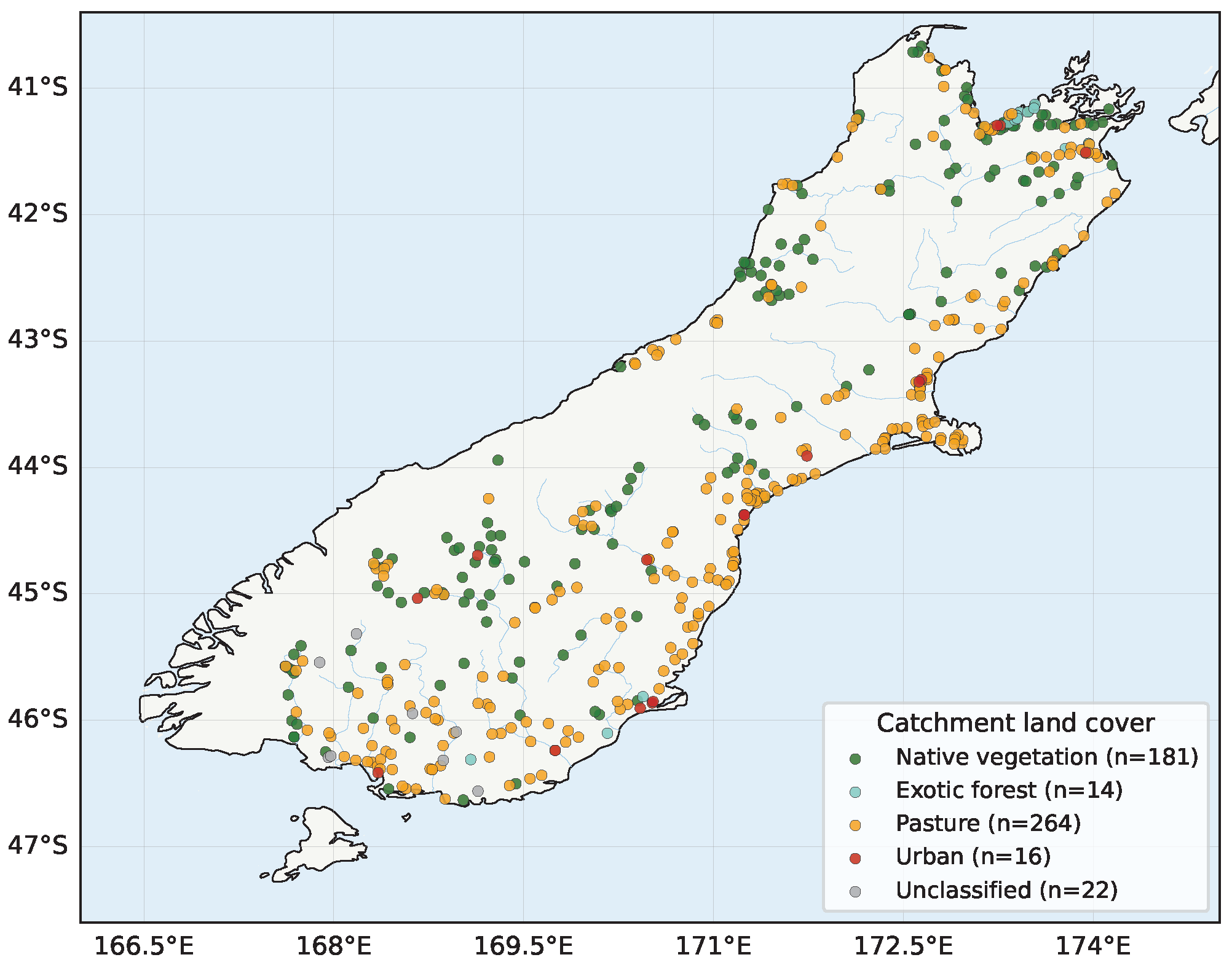
Figure 1. Distribution of the South Island river monitoring sites analysed in this study ( n = 497 ), coloured by dominant REC catchment land cover. The network spans a strong land-use gradient: native vegetation dominates the alpine and western interior, pasture the eastern plains and Southland lowlands, and the few urban sites cluster around the main centres. Land-cover classes describe dominant upstream catchment cover rather than land use at the sampling point (Section 2.1.2).
Water 18 02273 g001
Figure 2. Temporal data coverage of the labelled E. coli dataset. (a) Number of labelled site-years per year, 2004–2024, stacked by dominant catchment land cover; the dashed line marks the temporal train–test boundary used in the forecast evaluation (Section 3). (b) Distribution of the number of observations per site-year prior to the minimum-count filter, showing a bimodal pattern of quarterly (∼4) and monthly (∼12) sampling; the dashed line marks the ≥9-observation retention threshold, which excludes quarterly sampled cells to ensure each retained annual statistic rests on sufficient observations, which excludes quarterly sampled cells to ensure each retained annual statistic rests on sufficient observations.
Water 18 02273 g002
Figure 3. E. coli worst-band (Band E) breach rate by dominant catchment land cover, as the percentage of labelled site-years in breach (site-year counts in parentheses). Breach prevalence rises monotonically along the land-use-intensity gradient; the dashed line marks the network-wide mean (39.2%). Unclassified catchment site-years ( n = 79 ) are omitted from the per-class bars but retained in the network mean.
Water 18 02273 g003
Figure 4. Distribution of annual median E. coli concentration (log scale) by dominant catchment land cover, with each site-year coloured by its (four-statistic) breach status. Concentrations shift upward along the land-use-intensity gradient. The dashed line marks the NPS-FM band E median criterion (>260 cfu/100 mL); because a site-year can breach on the 95th-percentile or exceedance criteria at a lower median, the line is indicative of the median statistic alone and not a complete breach boundary—hence, the breaching site-years (red) that fall below it.
Water 18 02273 g004
Figure 5. Spearman rank correlation among the annual medians of the eleven monitored water–quality indicators, computed over all site-years with available indicator pairs. The nitrogen species (NO3–N, TON, DIN, TN) are near–collinear, the phosphorus and sediment indicators (DRP, TP, turbidity) form a second correlated block, and water clarity is strongly negatively correlated with turbidity ( 0.93 ). This redundancy motivates both the gradient–boosted ensemble, which is robust to correlated inputs, and the summing of SHAP contributions across correlated lagged features when interpreting forecast drivers (Section 2.6).
Water 18 02273 g005
Figure 6. Receiver operating characteristic curves for the one-, two-, and three-year E. coli forecasts on the temporal hold-out. The fixed 0.25 operating point and the persistence baseline are marked; at a false positive rate comparable to persistence, the model attains a higher true positive rate at every horizon.
Water 18 02273 g006
Figure 7. Confusion matrices for the one-, two-, and three-year E. coli breach forecasts on the temporal hold-out (target years 2019–2024), for the forecast model at the 0.25 operating point (top row), and the persistence baseline (bottom row). Cell values are site-year counts with row-normalised percentages in parentheses; the highlighted lower row (actual breaches) shows the model recovers a substantially larger share of breaches than persistence at every horizon (78.0%, 78.2%, and 76.5% against 68.2%, 68.3%, and 65.7%), at the cost of a higher false alarm rate in the upper row.
Water 18 02273 g007
Figure 8. Decision curves for the one-, two-, and three-year E. coli forecasts. Net benefit is plotted against threshold probability for the forecast model and for the two model-free policies of flagging all sites and flagging none. The forecast dominates both alternatives across the range 0.15–0.75 at all three horizons; the 0.25 operating point used throughout is marked.
Water 18 02273 g008
Figure 9. Early-warning performance on currently compliant site-years. Bars show the proportion of emerging E. coli breach sites that are compliant at the origin year and subsequently enter the worst band (Band E) recovered by the model at one-, two-, and three-year horizons. Persistence recovers none of these transitions by construction.
Water 18 02273 g009
Figure 10. Annual median E. coli trajectories (log scale, shared axes) for four representative monitoring sites, illustrating the model’s behaviour across outcome types: a caught emerging breach (top left), a stable compliant site (top right), a persistent breach (bottom left), and a false alarm (bottom right). The grey band marks the temporal hold-out (target years 2019–2024); within it, each point is coloured by the one-year forecast (red = predicted breach, grey = predicted compliant), and the annotation gives the forecast probability where it falls between 0.02 and 0.98; forecasts at the extremes are indicated by marker colour alone. The dashed line is the NPS-FM band E median criterion (>260 cfu/100 mL); because a site-year can breach on the 95th-percentile or exceedance criteria at a lower median, some ringedpoints fall below this line.
Water 18 02273 g010
Figure 11. Reliability of the raw one-year E. coli forecast scores on the temporal hold-out: observed breach frequency against predicted probability by decile. Points on the diagonal indicate perfect calibration; the scores are well calibrated at the low end but over-confident from the middle of the range upward.
Water 18 02273 g011
Figure 12. One-year forecast discrimination (AUC) within each land-cover class. Estimates for native vegetation and pasture sites rest on adequate sample sizes; the urban and exotic forest values are shown for completeness but derive from few site-years and should be read with caution.
Water 18 02273 g012
Figure 13. Feature attribution for the one-year forecast, as mean absolute SHAP value summed across the four lags and trend of each indicator (dark bars) and for the static catchment and status features (grey bars), on the temporal hold-out. The forecast is driven overwhelmingly by a site’s own recent E. coli history, followed at a distance by pH and turbidity. The low contribution of the binary current-breach flag (0.13) relative to the continuous indicators shows the model draws its signal from the recent water-quality trajectory rather than from present compliance status alone—the mechanism that allows it to anticipate transitions that a persistence rule cannot.
Water 18 02273 g013
Figure 14. Forecast E. coli compliance status across South Island river monitoring sites for 2027. Sites forecast to enter the worst band (Band E) are distinguished from those forecast to comply, and the 51 currently compliant sites forecast to degrade to breaching by 2027 are ringed, locating emerging risk for monitoring prioritisation.
Water 18 02273 g014
Figure 15. Composition of the 2025–2027 forward forecast by probability band, across the 412 sites with a valid 2024 origin record. Sites are divided into those forecast compliant (probability below the 0.25 operating threshold), those flagged marginally (0.25–0.5), and those flagged with high confidence (≥0.5). The high-confidence group varies without trend across horizons, while the marginal group contracts at the three-year horizon, showing that the decline in total flagged sites arises among borderline cases rather than from a uniform reduction in forecast risk.
Water 18 02273 g015
Table 1. Distribution of South Island monitoring sites across the four LAWA dominant land-cover classes derived from the River Environment Classification.
Land-Cover ClassSites (n)Share (%)
Native vegetation18136.4
Exotic forest142.8
Pasture26453.1
Urban163.2
Unclassified224.4
Total497100
Table 2. E. coli worst attribute band (Band E) criteria under the NPS-FM 2020. A site-year is labelled a breach if any single criterion is met. Units are cfu per 100 mL.
Annual StatisticBreach Condition
Median>260
95th percentile>1200
Proportion of samples exceeding 540≥30%
Proportion of samples exceeding 260≥50%
Table 3. Predictor set used by the forecasting model. Temporal predictors are computed per indicator from annual medians; static predictors describe the catchment.
GroupDefinitionCount
Lagged levelsAnnual median at lags 0–3 (years of record), per indicator 11 × 4
Three-year trendMedian change over 3 preceding years of record, per indicator 11 × 1
Current breach statusBinary E. coli breach flag at origin year1
Static catchmentLand cover, region, latitude, longitude4
Total 60
Table 4. Hold-out forecasting performance by horizon (target years 2019–2024). AUC summarises threshold-free discrimination; balanced accuracy, precision, recall, and the false alarm rate are reported at the single fixed operating threshold of 0.25. Persistence balanced accuracy is threshold-independent; the majority-class baseline attains 0.500 by construction.
Metric1-Year2-Year3-Year
AUC (model) 0.844 0.847 0.836
Balanced accuracy (model, thr 0.25) 0.747 0.765 0.755
Balanced accuracy (persistence) 0.734 0.7310.719
Precision @ 0.25 0.60 0.62 0.62
Recall @ 0.25 0.78 0.78 0.77
False alarm rate @ 0.25 0.29 0.25 0.25
Table 5. Operating thresholds and decision analysis, one-year horizon (target years 2019–2024, n = 2079 , breach prevalence 0.356). The false alert rate is the share of issued alerts not followed by a breach. Net benefit is computed at the cost weight implied by each row’s threshold; compare across columns within a row, not down a column.
Thr.FlaggedRecallPrec.False-AlertNB ModelNB Flag-All
0.1511140.8300.5510.4490.2530.242
0.259600.7800.6010.3990.2160.141
0.358470.7320.6400.3600.1820.009
0.507150.6770.7010.2990.138 0.288
0.656260.6310.7460.2540.083 0.840
0.755720.6000.7760.2240.029 1.576
Table 6. Early-warning (transition) performance on currently compliant site-years. Persistence flags none of the emerging breaches by construction.
Quantity1-Year2-Year3-Year
Currently compliant site-years tested 1287 1161 1100
 of which crossed to breach 235 205 211
Emerging breaches caught (model) 113 108 103
Recall on emerging breaches (model) 0.48 0.53 0.49
Recall on emerging breaches (persistence)0.000.000.00
Precision (model)0.37 0.40 0.39
False alarms among stable sites 195 164 163
Table 7. Early-warning performance of the full 60-predictor model against a six-predictor E. coli-only model on currently compliant hold-out site-years. Transitions recovered are reported at the common 0.25 threshold and at two matched operating points, since the two models place different score mass above a given probability.
Transitions Recovered1-Year2-Year3-Year
Transitions available235205211
Full model (thr 0.25)113108103
Reduced model (thr 0.25)140110106
Reduced, matched false positive rate1229098
Reduced, matched flagged count119100100
AUC advantage, full over reduced0.0010.0110.010
Table 8. Leave-region-out validation at the one-year horizon. Each row reports discrimination on one region’s hold-out site-years, first from the full-network model and then from a model trained with that region’s site-years excluded. Positive gaps indicate higher AUC without the region’s own training data.
RegionTest nBreach RateAUC (Full)AUC (Region Excluded)
Canterbury6110.3800.8490.861
Marlborough2150.2470.7200.711
Nelson1560.3010.7860.823
Otago5590.3060.8530.854
Southland1650.5520.8440.814
Tasman1770.3160.8940.872
West Coast1960.4590.8740.873
Disclaimer/Publisher’s Note: The statements, opinions and data contained in all publications are solely those of the individual author(s) and contributor(s) and not of MDPI and/or the editor(s). MDPI and/or the editor(s) disclaim responsibility for any injury to people or property resulting from any ideas, methods, instructions or products referred to in the content.