Urban Pluvial Flood Prediction in Huai’an City Based on a Transformer–GNN Fusion Model

Abstract

Urban pluvial flooding shows clear temporal accumulation, delayed response, and spatial heterogeneity. Better flood-depth prediction from a spatiotemporal coupling perspective can support urban flood risk identification and refined management. This study develops a spatiotemporal prediction model that integrates a Transformer and graph neural network (GNN). The Transformer module captures temporal dependencies in rainfall processes and flood-depth evolution. The graph attention network (GAT) represents spatial associations constrained by terrain, drainage networks, and neighboring spatial relationships. A fusion attention mechanism then adaptively couples temporal and spatial features. This study uses multi-source data, including hourly meteorological observations, terrain, land cover, drainage networks, and water-system data. It selects the heavy rainfall event caused by Typhoon In-Fa in Huai’an City in July 2021 as a typical case. The study analyzes the temporal evolution of regional average flood depth and the spatial differentiation of inundated grid cells at the municipal scale. The results show three main findings. First, during the typical heavy rainfall event, regional average flood depth follows a continuous process of low-level stability, sustained rise, rapid increase, delayed peak, slow recession at a high level, and rapid recession. The flood peak lags behind the rainfall peak by about 3 h. This result indicates clear accumulation and delayed response in urban pluvial flooding. Second, at the municipal scale, inundated grid cells show a pattern of concentrated distribution in urban built-up areas, secondary distribution in county-level built-up areas, and scattered distribution in non-construction land. Different depth grades also show clear hierarchical differentiation. Mild and moderate inundation covers a wider area. Medium-high inundation concentrates locally. High-grade inundation appears as a small number of nested high-value cells. Third, the spatial differentiation of medium- and high-grade inundated grid cells does not result from low-lying terrain or construction land alone. It forms under the combined effects of low-lying terrain, local relative depressions, and impervious surfaces in construction land. This pattern shows clear built-up-area clustering, grade differentiation, and land-cover correspondence. The results provide methodological support and decision references for urban flood risk identification, grid-based risk management, and emergency dispatch during extreme rainfall.

1. Introduction

Urban pluvial flooding is a frequent hazard during rapid urbanization. It threatens residents, traffic operations, and infrastructure safety. Climate change and urban expansion can both increase runoff generation and flood exposure. Short-duration heavy rainfall can quickly cause street ponding, traffic disruption, and cascading losses in areas with insufficient drainage capacity. Therefore, studies on flood formation mechanisms, spatiotemporal patterns, and high-risk areas have strong theoretical and practical value [1,2,3,4].

Researchers have developed many methods for urban flood prediction. The main technical routes include physically based hydrodynamic simulation, data-driven modeling with traditional machine learning, and deep learning for complex feature mining. These methods differ in modeling logic, data demand, computational cost, and interpretability. They also serve different prediction tasks under different spatial scales and accuracy requirements [5,6,7,8].

Physically based hydrodynamic models simulate flood evolution by describing rainfall-runoff-drainage processes. They have strong physical interpretability and can represent the coupling among rainfall, terrain, soil, pipe networks, and surface flow. Therefore, researchers widely use them for detailed flood simulation in complex urban areas. However, these models require difficult parameter calibration and high computational cost. They also introduce uncertainty when they generalize complex urban surfaces. These limitations restrict their application in real-time warning and large-scale rapid prediction [5,9,10,11,12,13,14].

Traditional machine learning methods predict urban flooding by mining statistical relationships among historical rainfall, geomorphology, and inundation data. These methods usually have high computational efficiency and a relatively simple workflow. They can support rapid risk assessment and real-time mapping when sufficient samples are available. However, their feature-expression capacity is limited. They often struggle to represent nonlinear spatiotemporal evolution, long-term rainfall dependence, and spatial heterogeneity in drainage-controlled urban environments [6,15,16].

Deep learning methods can extract nonlinear features from high-dimensional data. They provide new tools for rapid flood prediction and surrogate modeling. Recent studies have used neural networks, topographic deep learning, and attention mechanisms to predict urban flood depth and inundation maps. These studies show better efficiency and generalization than many traditional approaches. However, deep learning still depends on high-quality samples and careful model design, especially when the target task requires interpretable emergency decision support [7,8,17,18].

Although convolutional neural networks (CNNs) have been widely used for flood mapping and image-based spatial prediction, their underlying grid-based convolution operations primarily capture local spatial patterns in regular raster structures. Urban hydrological processes, however, are strongly constrained by irregular drainage networks, hydraulic connectivity, and topological relationships among spatial units. These relationships are difficult to represent explicitly using conventional CNN architectures because neighboring pixels in geographic space do not necessarily correspond to actual hydraulic interactions. In contrast, graph neural networks (GNNs) directly model spatial entities as nodes and hydraulic connections as graph edges, enabling explicit representation of drainage-network topology, runoff-transfer pathways, and spatial dependency structures. Therefore, GNN-based frameworks are better suited for urban flood prediction tasks where flood propagation is governed by network connectivity rather than solely by Euclidean spatial proximity [19,20,21].

This study constructs an urban pluvial flood prediction model that integrates a Transformer and a graph neural network (GNN). The model uses temporal attention to capture rainfall-dependent temporal features and graph-structured modeling to represent urban spatial associations. Huai’an City has frequent heavy rainfall, low-lying terrain, and a complex river network. These conditions make it suitable for model validation. Therefore, this study selects the July 2021 heavy rainfall event in Huai’an City as a representative case and analyzes flood prediction and spatiotemporal evolution patterns [19,20,21,22,23].

2. Materials and Methods

2.1. Model Construction Strategy

Urban flood prediction is a complex spatiotemporal evolution problem. Multiple sources drive it, and strong nonlinear constraints shape it. Rainfall accumulation over time and urban spatial structure jointly affect flood formation and development. In real urban environments, rainfall processes show nonstationarity and long-memory behavior. Drainage-network connectivity, terrain relief, and land-cover conditions also constrain the spatial distribution and propagation of flooding. Therefore, a model that uses only the temporal dimension or only the spatial dimension cannot fully describe the real evolution of urban flooding [1,2,23,24,25].

Existing urban flood prediction methods do not fully coordinate temporal-dependence modeling and spatial-structure modeling. To address this gap, this study builds a prediction framework that integrates Transformer and GNN. The framework includes three components: temporal evolution representation, spatial-structure constraint modeling, and spatiotemporal feature fusion. This design follows recent progress in attention-based time-series forecasting, graph learning, and spatiotemporal flood nowcasting [18,19,20,21,22,23].

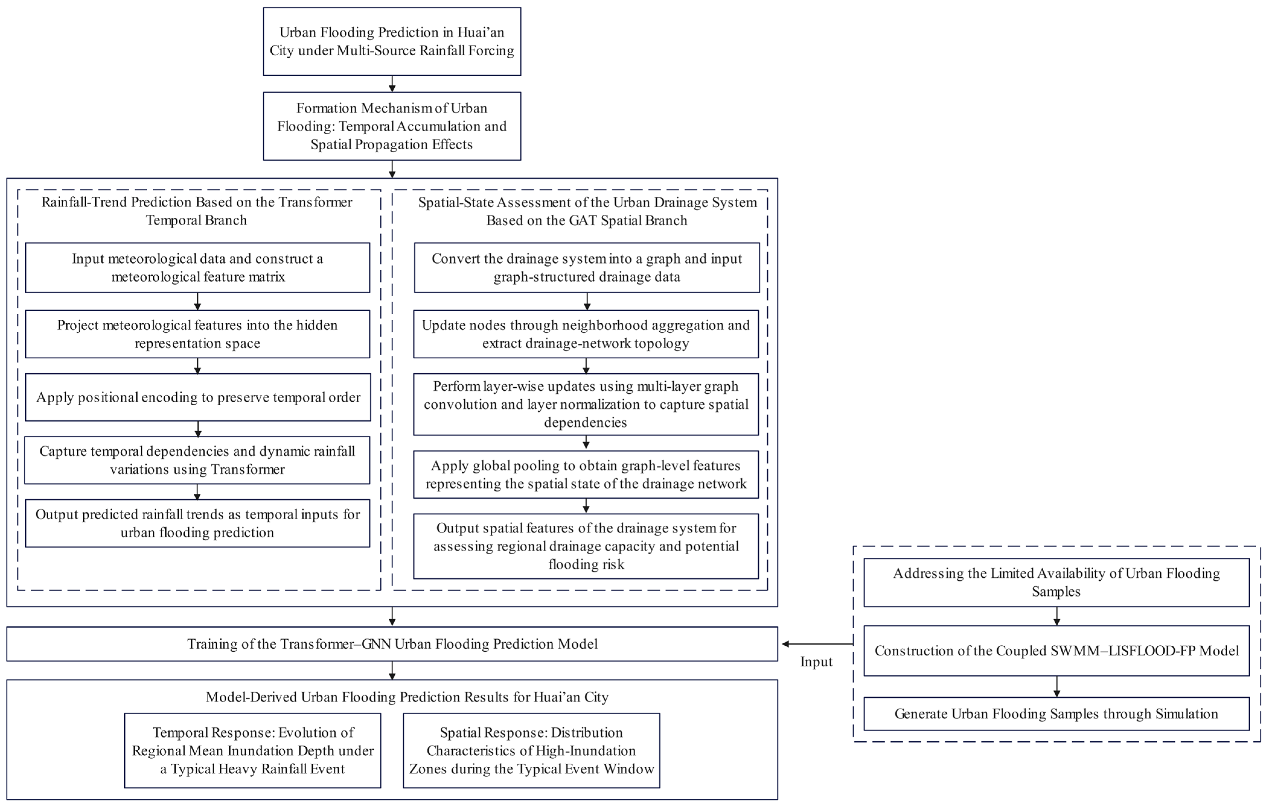
Figure 1 shows the model construction strategy. The framework follows the physical mechanism of urban flooding. It first decomposes flood evolution into two key dimensions. The temporal dimension describes dynamic changes in water depth. The spatial dimension describes runoff-path associations. The temporal model captures rainfall-driven changes in water depth. The graph model captures spatial convergence paths determined by terrain and drainage-network topology. The attention mechanism then adaptively fuses the two types of physical features. This allows the model to follow flood-related physical constraints while mining nonlinear relationships in the data [5,9,10,11,12,13,14,22,23].

2.2. Temporal Feature Model for Urban Flood Prediction

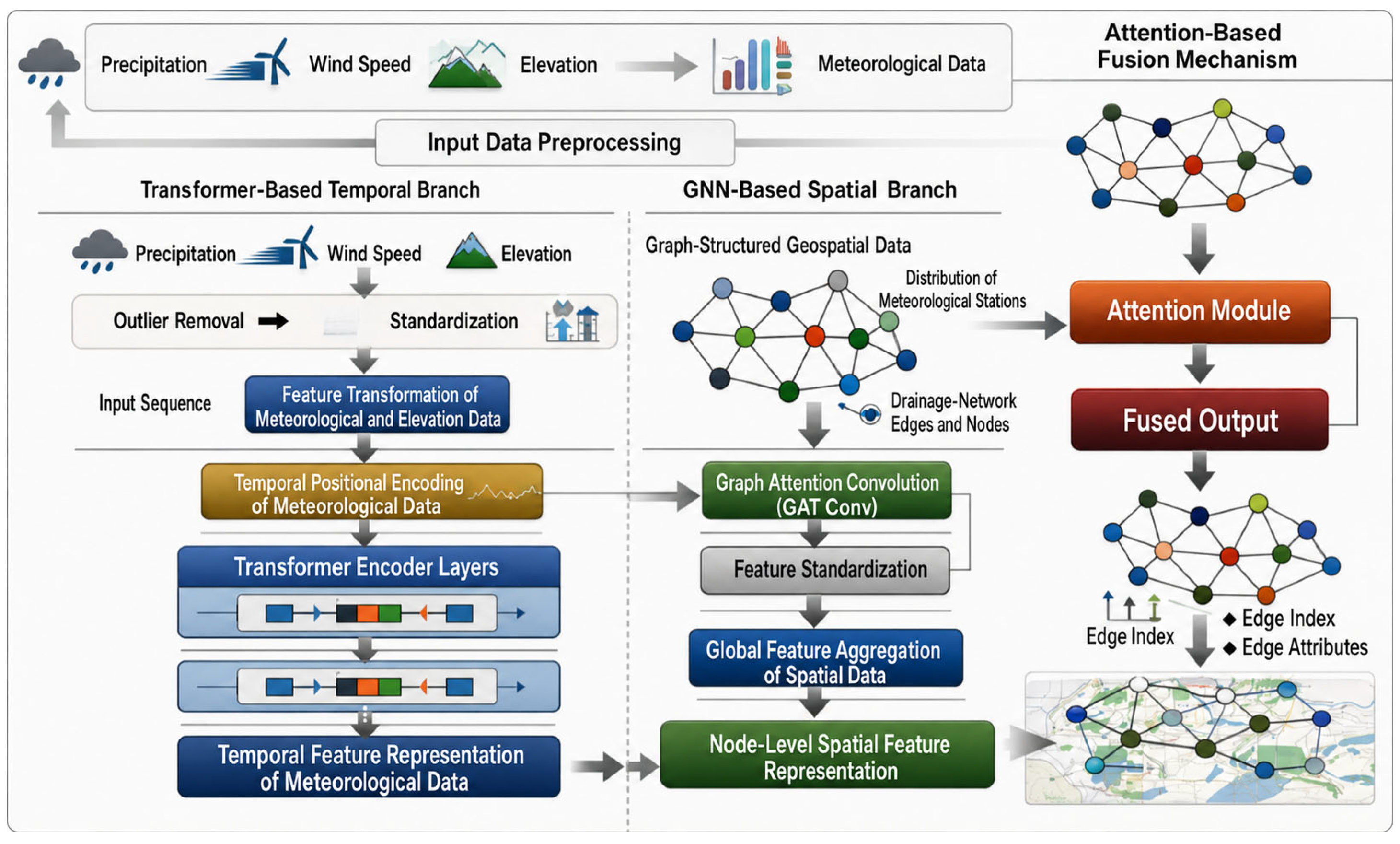
Urban flooding does not respond only to instantaneous rainfall. It evolves dynamically under the combined control of rainfall intensity, rainfall duration, and antecedent rainfall accumulation. During continuous rainfall or strong convective weather, previous rainfall affects surface water content, runoff generation capacity, and drainage-system load. These effects can change later flood development. As a result, urban flooding shows temporal accumulation, long-term dependence, and delayed response. A key task is to mathematically represent the temporal dependence of rainfall and related drivers. This task directly affects flood prediction accuracy (Figure 2) [22,24,25,26].

To represent the temporal dependence of flood evolution, this study constructs a temporal input feature set. Let the input feature vector at time t be $x_t$. It contains temporal drivers that directly affect flooding, such as rainfall amount at time t, rainfall intensity, and antecedent accumulated rainfall that reflects previous water storage. A sliding time window with length T yields a continuous temporal feature matrix [24,25]:

$$X = [x_{t-T+1},x_{t-T+2},x_t]$$

(1)

In Equation (1), the temporal matrix $X$ contains observations of key drivers from time t − T + 1 to time t. It aims to extract historical information from continuous rainfall inputs that affect the current inundation state. This structure represents two key temporal features. The first is the continuous change in the rainfall process over time. The second is the lasting effect of antecedent conditions, such as soil saturation and residual drainage-network capacity, on the current flood state. These features provide the input basis for later temporal-dependence modeling.

The temporal branch introduces the Transformer temporal self-attention mechanism. It quantifies how input features at different historical time steps affect the flood state at the prediction time. Unlike recurrent structures that rely on step-by-step propagation, temporal self-attention directly builds associations between any two time steps. It is more suitable for representing long-term dependence caused by continuous rainfall, delayed peaks, and cumulative response in urban flooding. Specifically, the temporal input matrix first maps to query (Q), key (K), and value (V) vectors through linear transformations [22,26]:

$$Q = X{W}_Q, K = X{W}_K, V = X{W}_V$$

(2)

In Equation (2), $W_Q$, $W_K$, and $W_V$ are trainable parameter matrices. The query vector represents the model’s attention demand for the current prediction task. It asks which previous time steps mainly affect the current flood state. The key vector represents the identification information carried by rainfall features at each historical time step. It supports matching with the query. The value vector represents the specific information content at each historical time step. This mapping transforms the original temporal input into a high-dimensional representation for attention-weight calculation.

After obtaining Q, K, and V, the Transformer uses temporal self-attention to weight information from each historical time step. The main calculation is:

$$\mathrm{Attention}(Q,K,V) = \mathrm{softmax}\left({\displaystyle \frac{Q{K}^T}{\sqrt{d_k}}}\right)V$$

(3)

In Equation (3), the dot product between the current query and historical key vectors first measures similarity. Scaling and softmax normalization then generate attention weights. These weights indicate the relative importance of each historical rainfall feature for predicting the current flood state. The model then computes a weighted sum of all value vectors to form the output of the temporal branch. This process shows that historical rainfall inputs do not contribute equally to urban flood formation. The model can adaptively identify key historical stages, such as periods of concentrated heavy rainfall or earlier rainfall accumulation. In this way, the model captures temporal accumulation and delayed response at the hourly scale under heavy rainfall. Modeling global temporal dependence improves the recognition of long-term flood evolution under complex rainfall scenarios. It also provides a stable and reliable temporal feature basis for later spatiotemporal modeling [15,22,26].

2.3. Spatial Association Feature Model for Urban Flood Prediction

In the spatial dimension, urban flooding shows strong structural characteristics. Different areas are not independent. Drainage-network connectivity, terrain relief, and water-system layout jointly form complex spatial associations. Ponding in one local area may affect adjacent areas through pipe-network overflow, surface runoff convergence, or downstream water-level backwater. These processes can promote flood-risk propagation and clustering in space. Therefore, a model that uses only single-point attributes cannot fully represent spatial diffusion paths, clustering patterns, or neighborhood interactions [3,10,11,27,28].

To explicitly represent these spatial structural constraints, this study abstracts the study area as a graph G = (V, E). The set V represents spatial units or drainage-system nodes, such as key nodes in the drainage network. The set E represents physical or hydraulic links among these units, such as connecting pipes and surface runoff paths. Each node $V_i$ has a feature vector $h_i$ that quantifies water depth, geomorphology, drainage capacity, and related attributes. At layer l of the network, the feature vector of node i is denoted as $h_i^{\left(l\right)}$. In the model implementation, the spatial branch uses a graph attention network (GAT), rather than ordinary graph convolution, to propagate and update node features [19,20,21,23]. The spatial branch consists of multiple GATConv layers. This means that the model introduces explicit attention-weight allocation in the spatial dimension.

The GAT updates node features through neighborhood information propagation. Its general form is

$${\mathbf{h}}_i^{(l+1)}=\sigma \left(\sum _{j\in N\left(i\right)}{\alpha }_{\mathit{ij}}^{\left(l\right)}{\mathbf{W}}^{\left(l\right)}{\mathbf{h}}_j^{\left(l\right)}\right)$$

(4)

In Equation (4), the terms have the following physical meanings:

$N\left(i\right)$ denotes the neighborhood of node i. It includes upstream, downstream, and adjacent areas that have direct hydraulic links or runoff-transfer relationships with target area i. This neighborhood defines the direct spatial range of flood influence. It is an important source of risk propagation.

The trainable weight matrix ${\mathit{W}}^{\left(l\right)}$ performs linear transformation and feature mapping of neighborhood information according to node attributes. Under urban spatial heterogeneity, it helps the model extract the combined effects of terrain, drainage networks, and water-depth states on spatial propagation.

The nonlinear activation function $\sigma (·)$ represents complex nonlinear relationships in flood formation and evolution. These relationships include sudden overflow after a water-depth threshold, superposition of inflow from multiple paths, and uneven response caused by local drainage bottlenecks.

The coefficient ${\alpha }_{ij}$ in Equation (4) differs from the temporal self-attention weights discussed above. It is a neighborhood attention coefficient in the spatial graph attention mechanism. It dynamically quantifies the relative influence of neighboring node j on the flood-state update of target node i. The features of nodes i and j jointly determine this weight. It is essentially a local masked self-attention constrained by graph neighborhoods. The model does not build attention directly among all nodes. Instead, it assigns attention only among neighboring nodes that have actual connections. This design highlights key influence sources along local spatial propagation paths. For urban flooding, it can represent complex spatial interactions. Examples include downstream water-level backwater that blocks upstream drainage, terrain-controlled runoff convergence, and strong constraints imposed by drainage bottleneck nodes on upstream areas. Thus, the coefficient reflects the influence strength during spatial transmission of flood risk.

This spatial graph attention propagation mechanism mathematically simulates flood-risk diffusion and superposition in urban space. During prediction, the model considers neighboring water-depth states, drainage connectivity, and spatial neighborhood influence. It can therefore represent spatial propagation and clustering of flooding. The core of this section is not general spatial feature extraction. It is GAT-based spatial neighborhood attention modeling. This mechanism supports the interpretation of spatial heterogeneity and formation mechanisms in urban flooding. It also provides a reliable spatial representation for the later fusion of temporal and spatial features [19,20,21,23].

2.4. Fusion Modeling Framework for Temporal and Spatial Features

Urban flood evolution results from the coupling between temporal evolution and spatial structure. Flood risk depends on rainfall accumulation over time. It also remains constrained by urban spatial structure, such as drainage-network connectivity and terrain relief. A single modeling dimension cannot fully reflect this complex spatiotemporal interaction. Therefore, after obtaining the temporal feature representation $H_t$ and the spatial association feature representation $H_{\mathrm{s}}$, a unified collaborative modeling framework is needed. The temporal representation contains rainfall accumulation and delayed response. The spatial representation describes risk propagation and clustering under drainage-network and terrain constraints [1,2,24,25]. The framework integrates these two types of information and adaptively couples them.

Simple feature concatenation may introduce information redundancy. It may also allow one dimension to dominate prediction. To avoid this, this study introduces a fusion attention mechanism to adaptively weight temporal and spatial features. This mechanism simulates the dynamic balance between temporal and spatial drivers of water depth. The attention used here differs from temporal self-attention and spatial graph attention. It acts on high-level feature representations from the two branches. Its main role is not to mine dependencies within a sequence. Instead, it dynamically evaluates the relative contribution of temporal drivers and spatial structure to prediction under the current sample scenario [18,19,22,23]. The model first concatenates the two features into a joint representation. It then uses a learnable parameter matrix to calculate fusion attention weights.

$$[{\alpha }_t,{\alpha }_s]=\mathit{softmax}\left(W_f\right[H_t;H_s\left]\right)$$

(5)

In Equation (5), $[·;·]$ denotes vector concatenation. The calculated weights quantify the relative contributions of temporal drivers, such as rainfall intensity, duration, and antecedent accumulation, and spatial structure factors, such as drainage capacity, terrain conditions, and neighboring ponding effects. This design reflects the dynamic changes in dominant flood-forming factors. For example, in a short-duration heavy rainfall event, spatial drainage capacity may become the main limitation for rapid runoff and ponding. During continuous rainfall or when antecedent soil saturation is high, rainfall accumulation may become more important. Therefore, Equation (5) describes a fusion attention mechanism that allocates contributions between the temporal and spatial branches.

Based on these fusion attention weights, the model weightedly fuses spatiotemporal features and obtains an integrated collaborative representation:

$$H_{\mathit{ts}} = {\alpha }_t{H}_t + {\alpha }_s{H}_s$$

(6)

In Equation (6), the model realizes a dynamic collaborative expression of temporal information and spatial structure. It does not preset the contribution ratio of the two branches. Instead, it adjusts attention to different physical processes according to rainfall features, antecedent accumulation, and urban underlying-surface conditions. The representation is not a simple linear sum. It is a spatiotemporal joint representation produced under fusion attention. This modeling approach better matches urban flood evolution, where multiple factors interact and dominant mechanisms vary by scenario. It helps improve prediction stability and generalization under complex flood scenarios. It also provides a stronger collaborative feature basis for water-depth prediction [17,18,19,22].

2.5. Selection of Factors Affecting Flood Depth

Urban flooding is controlled by rainfall, topography, surface properties, drainage-system conditions, and water-system characteristics. No single factor can fully explain its formation. Therefore, this study builds an indicator system that includes meteorological, terrain, drainage-system, land-cover, and water-system variables (

Table 1. Indicator system for urban-flood impact assessment.

Category	Indicator	Meaning	Data Source	Model Input Type
Meteorological factors	Hourly rainfall (PRCP)	Total rainfall per unit time; direct driver of urban flooding	Meteorological-station observations	Temporal input (Transformer)
Meteorological factors	Rainfall intensity	Intensity variation during the rainfall process	Calculated from station data	Temporal input
Meteorological factors	Antecedent cumulative rainfall	Rainfall accumulation and antecedent surface wetness	Historical rainfall sequence	Temporal input
Topographic conditions	Elevation	Terrain height and ponding potential	DEM data	Spatial node feature (GNN)
Topographic conditions	Slope	Surface-runoff velocity and direction	DEM data	Spatial node feature
Topographic conditions	Aspect	Local surface moisture and evaporation conditions	DEM data	Spatial node feature
Drainage system	Drainage-network connectivity	Drainage-network structure and water-transfer pathways	Urban drainage-network data	Graph-edge information
Drainage system	Spatial locations of drainage nodes	Distribution of key drainage nodes	Drainage-network data	Graph node attribute
Land-cover conditions	Impervious-surface ratio	Degree of surface hardening	Remote-sensing/land-use data	Spatial node feature
Land-cover conditions	Road density	Urban development intensity and runoff-generation potential	GIS road data	Spatial node feature
Water-system conditions	Water-system line density	Length of rivers and channels per unit area	Water-system line data for Huai’an City	Spatial node feature
Water-system conditions	Water-surface proportion	Proportion of lakes, reservoirs, and other water bodies	Water-system polygon data for Huai’an City	Spatial node feature

). The selection of indicators was guided by the physical mechanisms governing urban pluvial flooding and by findings reported in previous hydrological and urban-flood studies.

Urban flooding is generated through the interaction of rainfall forcing, surface runoff generation, flow routing, drainage conveyance, and water storage processes. Therefore, the indicator system was designed to represent these key components of the flood-generation mechanism from both temporal and spatial perspectives.

Meteorological variables (hourly rainfall, rainfall intensity, and antecedent cumulative rainfall) were selected because rainfall serves as the primary driving force of flood generation. These variables jointly characterize rainfall magnitude, temporal variability, and cumulative wetting effects that influence runoff production [24,25].

Terrain variables, including elevation, slope, and aspect, were incorporated because topography controls surface-water accumulation, flow direction, and runoff concentration. Low-lying areas and local depressions are generally more susceptible to inundation during heavy rainfall events [27,28].

Drainage-system indicators, including drainage-network connectivity and drainage-node locations, were selected to represent the efficiency of urban drainage infrastructure and the pathways through which floodwater is conveyed and redistributed. These variables capture potential conveyance bottlenecks and network-level hydraulic behavior [5,9,10,11,12,13,14].

Land-cover indicators, including impervious-surface ratio and road density, were used to characterize urbanization intensity and runoff-generation potential. Highly impervious surfaces reduce infiltration capacity and accelerate runoff concentration, thereby increasing flood susceptibility [1,4,27].

Water-system indicators, including river-network density and water-surface proportion, were incorporated because rivers, lakes, and channels regulate flood storage and discharge processes and may either mitigate or aggravate local inundation under extreme rainfall conditions [3,4].

In the proposed model framework, meteorological indicators are treated as temporal inputs to the Transformer branch, whereas terrain, drainage-system, land-cover, and water-system indicators are used as spatial node features in the GNN branch. Drainage-network connectivity is further utilized as graph-edge information to represent the underlying network topology [1,2,3,4,24,25,27,28].

2.6. Sample Collection and Preprocessing

2.6.1. Sample Collection

Because observed urban-flood data in Huai’an City are limited in temporal continuity and spatial coverage, this study constructs the sample set by combining observed information with model simulation. High-resolution observed inundation data are difficult to obtain at city scale; therefore, hydrological and hydrodynamic simulations are used to generate flood-depth samples under different rainfall scenarios, with available observations used for constraint and validation [7,8,14,16].

Considering the low-lying terrain, dense river network, and complex drainage system of Huai’an City, a single model cannot adequately represent both pipe-network hydraulics and surface inundation. This study therefore couples the Storm Water Management Model (SWMM), a one-dimensional drainage-network model, with LISFLOOD-FP, a two-dimensional surface hydrodynamic model. SWMM simulates pipe-network runoff, conveyance, and overflow, whereas LISFLOOD-FP describes surface runoff concentration and inundation diffusion. By linking pipe-node overflow with two-dimensional surface cells, the coupled system represents key hydrodynamic processes such as drainage discharge, surface storage, and backwater effects from external rivers [5,9,10,11,12,13].

Model inputs include a vector-constrained digital elevation model (DEM), land-use and impervious-surface data, drainage-network topology, and rainfall scenarios covering both design storms and historical heavy-rainfall events. Key hydraulic parameters are calibrated and tested for sensitivity to improve simulation stability and reliability (

Table 2. Key parameter-calibration results.

Parameter Category	Parameter	Calibrated Value	Reasonable Range	Sensitivity
Infiltration parameter	Horton maximum infiltration rate f0 (mm/h)	3.8 mm/h	2–15 mm/h	High
Infiltration parameter	Horton final infiltration rate fc (mm/h)	1.2 mm/h	0.5–5 mm/h	Medium
Infiltration parameter	Horton decay coefficient k	2.1	1–4	Medium
Pipe-network hydraulic parameter	Pipe Manning roughness coefficient n	0.015	0.011–0.017	High
Pipe-network hydraulic parameter	Manhole loss coefficient	0.60	0.4–0.8	Medium
Surface hydrodynamic parameter	Surface Manning roughness	0.020	0.015–0.040	Medium
Surface hydrodynamic parameter	Surface roughness in built-up areas	0.035	0.020–0.050	Low-medium

) [12,13,24,25].

The qualitative sensitivity rankings reported in Table 2 are derived from previous urban-flood modeling studies and practical calibration experience commonly adopted in SWMM- and hydrodynamic-model applications [5,10,13]. Parameters classified as “High” sensitivity are generally recognized as exerting substantial influence on runoff generation, hydraulic routing, or inundation depth, whereas “Medium” and “Low-Medium” sensitivity parameters typically have comparatively smaller effects on model outputs. The sensitivity levels reported here are intended to guide parameter calibration and interpretation and do not represent the results of a formal quantitative sensitivity analysis conducted in this study.

Independent validation against historical storm events yielded a Nash-Sutcliffe efficiency (NSE) of 0.68 for simulated inundation depth. Urban flooding is strongly affected by terrain details, heterogeneous land cover, and drainage-network structure. In this context, the validation result indicates acceptable performance for sample generation. The simulated high-resolution inundation results also show good consistency with available water-depth records. These samples are therefore suitable for training and testing the Transformer–GNN model [9,14,29].

To enhance the generalization capability of the proposed Transformer–GNN framework, the training dataset was generated from hydrodynamic simulations driven by diverse rainfall scenarios derived from long-term rainfall records. These rainfall inputs encompass a wide range of rainfall intensities, durations, cumulative depths, and temporal rainfall patterns. Consequently, the model was exposed to substantially more hydrological variability than the single Typhoon In-Fa event presented in the Results Section 3. The Typhoon In-Fa event was selected solely as a representative case study for illustrating model performance and spatial inundation dynamics.

2.6.2. Simulation-Based Training Sample Limitations

Although the calibrated SWMM–LISFLOOD-FP model achieved an acceptable validation performance (NSE = 0.68), approximately 32% of the variance in observed inundation dynamics remains unexplained. This residual uncertainty is mainly associated with rainfall-input errors, parameter-calibration uncertainty, terrain representation, drainage-network abstraction, and simplifications of hydraulic processes.

However, the purpose of the hydrodynamic model in this study is not to reproduce every local inundation detail exactly, but to generate physically consistent spatiotemporal samples that capture the dominant mechanisms of urban flood formation and propagation. Consequently, the proposed Transformer–GNN model learns generalized relationships between rainfall forcing, environmental conditions, and inundation responses rather than directly replicating individual simulation errors.

Nevertheless, systematic biases in the simulation results may propagate into the training dataset and affect prediction accuracy in areas characterized by complex hydraulic interactions or limited observational constraints. Therefore, the predictive performance of the Transformer–GNN model should be interpreted within the uncertainty bounds of the underlying hydrodynamic simulations. Given the scarcity of high-resolution observed inundation datasets at the city scale, the achieved NSE value is considered sufficient for constructing representative training samples. Future studies will incorporate additional observed flood records and multi-source monitoring data to further reduce uncertainty and improve model reliability.

In addition, model evaluation in this study is based primarily on the July 2021 Typhoon In-Fa event, which was selected because it represents one of the most severe and well-documented urban flooding events in Huai’an City. This event provides relatively complete rainfall observations, hydrodynamic simulation outputs, and inundation records for model development and validation. Although the event includes pronounced temporal rainfall variability and complex spatial inundation patterns, validation based on a single event cannot fully demonstrate model generalization under different rainfall characteristics and hydrological conditions. Future studies will incorporate multiple rainfall events with varying intensities, durations, and spatial distributions to further evaluate the robustness, transferability, and generalization capability of the proposed Transformer–GNN framework.

2.6.3. Data Preprocessing

To ensure consistency and reliability across temporal and spatial modeling, flood, meteorological, topographic, and drainage-network data were systematically preprocessed. The workflow includes data quality control, feature construction, and spatiotemporal alignment. These steps reduce noise, coordinate inconsistencies, and scale differences among data sources [14,24,25].

Data quality control involved checking raster projections, vector geometry validity, and drainage-network node-edge connectivity. Potential outliers in historical inundation records were detected using the Isolation Forest algorithm. The method measures anomaly degree by randomly partitioning the feature space. Its anomaly score can be written as follows [30]:

$$s(x) = 2^{{\displaystyle \frac{E\left(\mathrm{h}\right(x\left)\right)}{c\left(n\right)}}}$$

(7)

Samples with anomaly scores above a prescribed threshold were treated as outliers. Spatially unreasonable points were removed using administrative boundaries, and time fields were standardized to ensure temporal continuity. These operations reduce the influence of isolated errors on model training and validation [30].

Meteorological driving variables were extracted from rainfall data. DEM and slope rasters were spatially matched to flood locations to represent local terrain differences. The raster extraction process can be written as follows [24,25]:

$$z_i=f(x_i,y_i)$$

(8)

A nearest-neighbor interpolation method was used to fill a small number of missing values. This method keeps local spatial consistency when data gaps are limited:

$$\widehat{x } ={\displaystyle \frac{1}{K}}{\displaystyle \sum _{j=1}^K}{x}_j$$

(9)

To capture nonlinear interactions between rainfall and terrain, interaction features between precipitation and topographic factors were constructed. These terms help the model represent the fact that the same rainfall can produce different inundation responses under different elevations, slopes, and land-cover conditions [24,25,27,28]:

$$X_{\mathit{int}} = P \times H$$

(10)

Because flood-depth variables often exhibit skewed distributions, the target variable was log-transformed to reduce the influence of extreme values during model training. Such transformations are commonly used in data-driven hydrological modeling when target distributions include rare high-value events [6,7,8]:

$$y^{\prime }=\log (y+1)$$

(11)

For numerical stability, drainage-network data were abstracted into a graph $G=(V,E)$. Nodes represent pipe-network nodes or spatial units. Edges represent pipe connections or hydraulic links. Node coordinates and node attributes were standardized before model training. The whole preprocessing workflow used fixed random seeds to ensure reproducible experiments [23].

2.7. Comparative Experimental Setup

To further evaluate the effectiveness of the proposed Transformer–GNN framework, comparative experiments were conducted using three representative deep-learning models, namely Long Short-Term Memory (LSTM), Convolutional Neural Network (CNN), and U-Net. These models were selected because they represent different approaches for extracting temporal and spatial information in flood-prediction tasks. LSTM is widely used for hydrological time-series forecasting owing to its capability to capture temporal dependencies in sequential data. CNN has been extensively applied to flood prediction and environmental modeling because of its ability to extract local spatial features from gridded datasets. U-Net, an encoder–decoder convolutional architecture, has demonstrated strong performance in flood-inundation mapping and spatial prediction tasks by effectively integrating multi-scale spatial information [15,17,26].

To ensure a fair comparison, all benchmark models and the proposed Transformer–GNN model were trained and evaluated using the same dataset generated from the coupled SWMM–LISFLOOD-FP simulations. The same training, validation, and testing samples were adopted under a five-fold cross-validation framework. Model parameters were optimized independently to achieve stable convergence while maintaining comparable experimental conditions.

Model performance was evaluated using the coefficient of determination (R²), root mean squared error (RMSE), mean absolute error (MAE), and mean absolute percentage error (MAPE). R² was used to assess the goodness-of-fit between predicted and reference inundation depths, whereas RMSE and MAE quantified the magnitude of prediction errors. MAPE was used to evaluate relative prediction accuracy. Higher R² values and lower error metrics indicate better predictive performance.

The purpose of this comparative analysis is to assess whether the integration of Transformer-based temporal feature learning and graph neural network-based spatial topology representation can provide performance advantages over conventional sequence-based and convolution-based deep-learning architectures for urban flood-depth prediction.

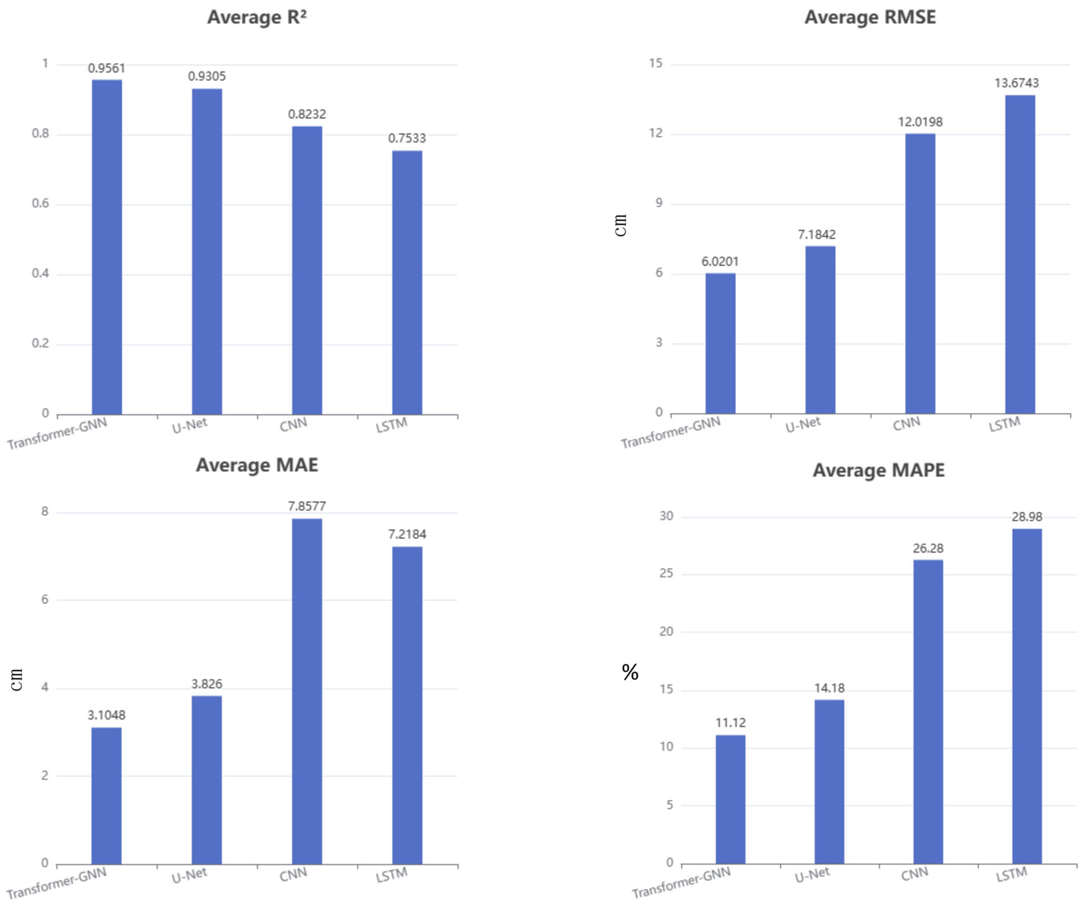
Figure 3 presents the comparative performance of different deep-learning models under five-fold cross-validation. The proposed Transformer–GNN framework achieved the highest prediction accuracy among all benchmark models, with an average R² of 0.9561, RMSE of 6.0201 cm, MAE of 3.1048 cm, and MAPE of 11.12%.

Compared with the LSTM model, the proposed framework improved the average R² by approximately 26.9% while reducing RMSE and MAE by 56.0% and 57.0%, respectively. Compared with CNN, the Transformer–GNN model achieved higher prediction accuracy and substantially lower prediction errors across all evaluation metrics. Although U-Net exhibited relatively strong predictive capability owing to its encoder–decoder structure and multi-scale spatial feature extraction, its average R² remained lower than that of the proposed framework, and all error metrics were consistently higher.

The superior performance of the proposed Transformer–GNN framework can be attributed to its ability to simultaneously capture temporal rainfall evolution and spatial topological relationships within the urban drainage system. The Transformer module effectively models long-range temporal dependencies in rainfall sequences, whereas the graph neural network explicitly represents connectivity and information propagation among drainage nodes. Consequently, the proposed framework provides a more comprehensive representation of urban flood-generation mechanisms than conventional sequence-based or convolution-based models.

Based on the above comparison results, the Transformer–GNN framework was selected as the prediction model for subsequent analyses of temporal inundation evolution and spatial inundation distribution during the representative heavy-rainfall event.

3. Results

This section uses the July 2021 heavy rainfall event influenced by Typhoon In-Fa as the representative event window. Based on the spatiotemporal fusion model, it analyzes the temporal response of average inundation depth and the spatial distribution of inundated grid cells in Huai’an City. The goal is to identify event-scale risk characteristics and provide support for urban flood management [1,2,3,14].

3.1. Temporal Characteristics of Regional Inundation During the Representative Heavy-Rainfall Event

3.1.1. Temporal Evolution of Regional Mean Inundation Depth

Regional mean inundation is a useful indicator of the overall flood response. It can reveal the stage relationship between rainfall input and water-depth response. This study therefore compares hourly rainfall with model-predicted mean inundation depth during the representative event window. The analysis focuses on peak response, duration, and recession characteristics [14,24,25].

Figure 4 shows the temporal relationship between regional mean inundation depth and hourly rainfall. Overall, the regional mean inundation process follows a continuous evolution: low-level stability, sustained rise, rapid increase, delayed peak, slow recession at a high level, and rapid recession. This process indicates a clear lag between rainfall forcing and flood-depth response.

Delayed peak. In the early stage from 06:00 to 12:00 on 27 July, regional mean inundation remained low and fluctuated weakly. With increasing rainfall, inundation entered a sustained rising stage. From 03:00 to 04:00 on 28 July, the curve slope increased sharply, indicating stronger runoff generation and convergence. Hourly rainfall peaked at 04:00 on 28 July, while regional mean inundation continued to rise and peaked at 07:00. The inundation peak lagged behind the rainfall peak by about 3 h. This lag reflects accumulation, routing time, and drainage-system response [14,24,25].

Slow recession at a high level. From 07:00 to 12:00 on 28 July, regional mean inundation entered a slow recession stage. Although the peak had passed, water depth decreased slowly and the curve formed a near-plateau shape. This indicates that runoff supply, drainage constraints, and local storage jointly maintained high water levels after the rainfall peak.

Rapid recession. After 12:00, regional mean inundation decreased more rapidly. The curve shifted from a gentle decline to a clear downward trend. Water depth fell continuously over a short period. Compared with the high-level recession stage, the unit-time recession rate was higher, indicating that runoff supply weakened and the drainage system and river channels began to discharge accumulated water more effectively.

3.1.2. Mechanisms of the Temporal Evolution of Regional Mean Inundation

The temporal evolution of regional mean inundation results from the joint effects of rainfall input, surface runoff generation, drainage capacity, and local storage. The representative event shows that urban flood processes have both cumulative and delayed characteristics. These characteristics are closely related to rainfall duration, antecedent wetness, topographic storage, and pipe-network conveyance [5,9,10,11,12,13,14,24,25].

Low-level stability. In the early stage, hourly rainfall was relatively weak. Rainwater was partly absorbed by surface depression storage, infiltration, and the existing drainage capacity. Therefore, regional mean inundation did not increase clearly.

Sustained rise. As rainfall continued and gradually intensified, inundation increased steadily. Three mechanisms explain this process. First, antecedent storage space was progressively occupied. Low-lying areas, surface depressions, and pipe-network storage approached their capacity. Second, surface runoff generation increased because soil water content rose and infiltration capacity declined. Third, upstream and surrounding runoff continued to converge toward lower areas. These processes pushed the inundation curve upward [4,24,25,27,28].

Rapid surge. Between 03:00 and 04:00 on 28 July, intense rainfall combined with antecedent inflow substantially increased surface runoff generation and convergence. Regional mean inundation shifted from sustained rise to rapid surge. This stage indicates that the flood response became stronger when rainfall intensity exceeded the combined regulation capacity of storage and drainage.

Delayed peak. The delayed peak reflects three main factors. First, rainfall must move through surface-flow and drainage-conveyance pathways before affecting inundation locations. Second, storage in depressions and pipe networks delays the conversion from rainfall to visible ponding. Third, drainage systems and external water levels can prolong high water levels, especially in low-lying river-network cities [5,9,10,11,12,13,14].

Slow recession at a high level. From 07:00 to 12:00 on 28 July, inundation depth decreased slowly. This high-level recession reflects both cumulative and lag effects. Surface runoff from upstream and surrounding areas still supplied water to lower areas. Some pipe sections may have remained under high load. Therefore, water depth stayed high even though rainfall had weakened.

Rapid drawdown. After 12:00, rainfall had largely ceased, runoff supply declined, delayed inflow from upstream and surrounding areas weakened, and drainage-system hydraulic gradients recovered. Water accumulated in surface depressions and pipe networks was discharged more quickly. This explains the accelerated decline of the regional mean inundation curve.

3.1.3. Implications of Regional Inundation Evolution for Emergency Response

Off-peak response window. The lag between rainfall peak and inundation peak indicates that the most dangerous flood condition did not coincide with the most intense rainfall. Emergency managers should not lower response levels immediately after rainfall weakens. Pumping, traffic control, inspection, and public warning should continue through the delayed peak period [2,3,14].

Quantifying the duration of risk exposure. The prolonged high-level recession determines how long high-risk water levels persist. This is critical for evaluating traffic disruption, underground-space safety, and the timing of recovery operations. The duration of high water levels can support staged emergency response and post-event drainage scheduling.

Identifying potential extreme-risk intervals. The P90 predicted curve is higher than the mean curve, indicating a distributional response under more extreme modeled conditions. This can help decision makers identify conservative control intervals and reserve emergency capacity for uncertain or more severe rainfall scenarios.

3.2. Spatial Distribution of High-Inundation Zones During the Representative Event Window

3.2.1. Overall Spatial Pattern and Inundation-Level Differentiation

To reveal the spatial response of urban flood risk, the trained Transformer–GNN model was used to predict inundation processes for spatial units within the representative event window. Figure 5, Figure 6, Figure 7 and Figure 8 show the inundation-depth distribution, elevation background, land-cover pattern, and inundation-depth proportions under different land-cover types. These figures together support spatial interpretation of high-inundation zones [3,16,17,18,19,20,21,28].

(1)

City-scale spatial pattern.

Figure 5 and Figure 7 show that inundated grid cells were unevenly distributed during the event. They did not spread randomly across Huai’an City. Instead, they clustered in the main built-up area, appeared secondarily in county-level built-up areas, and occurred sporadically on non-construction land. This pattern reflects the joint effects of urban development intensity, impervious surfaces, local depressions, and drainage capacity [16,18,19,20,21,27,28].

(2)

Spatial differentiation of inundation levels.

Inundation-depth grades showed clear hierarchical differentiation. Cells with depths of 15–30 cm covered a relatively wide area. Cells with depths of 30–50 cm and ≥50 cm were more localized. They mainly appeared in built-up areas and local low-lying units. This result indicates that higher-risk cells were embedded within broader mild-to-moderate inundation areas [3,17,28].

(3)

Terrain constraints.

Figure 6 shows that Huai’an City has generally low and flat terrain. Elevation variation is limited, and many areas have gentle surface gradients. These conditions provide a background for water accumulation. However, inundated cells did not appear in all low-lying areas. Therefore, elevation alone cannot explain the spatial pattern [4,27,28].

(4)

Land-cover response differences.

Figure 5, Figure 7 and Figure 8 show that inundation-depth distributions differ among land-cover types. Built-up land and impervious surfaces are strongly associated with medium-high inundation. Agricultural land, forest and grassland, and open water areas show different inundation-depth proportions because they differ in infiltration, roughness, storage, and drainage conditions. This result highlights the role of land-cover structure in runoff generation and flood concentration [1,4,27].

(5)

Integrated spatial characteristics.

Overall, high-inundation zones during the event exhibit three key characteristics: spatial clustering, hierarchical differentiation, and factor correspondence. The spatial distribution is closely related to built-up areas and local low-lying terrain. However, high-risk locations result from multiple coupled conditions rather than a single factor.

3.2.2. Formation Mechanisms of High-Inundation Zones Under the Combined Effects of Terrain and Land Cover

The formation of high-inundation zones during the event is not controlled by a single factor. It is produced by interactions among rainfall input, terrain, land cover, built-up space, drainage-system capacity, and the regional water-system setting. These interactions explain why high-inundation zones cluster in some urban cells while other low-lying areas show lower water depths [1,3,24,25,27,28].

Basic terrain constraint. Terrain is a fundamental factor affecting inundation. Huai’an City is generally low and flat, and many areas have limited elevation variation and gentle slopes. Such terrain slows surface runoff and promotes local storage. Local relative depressions therefore provide the physical basis for medium- and high-grade inundation [27,28].

Regulation of runoff generation by land cover. Land cover affects interception, infiltration, surface roughness, and runoff generation. Impervious built-up land converts a large proportion of rainfall into surface runoff. It also reduces infiltration and shortens concentration time. As a result, built-up areas have greater potential for rapid ponding under heavy rainfall [1,4,27].

Combined built-up-area convergence and drainage stress. High-inundation zones in the main urban area and county-level urban areas are closely related to runoff pathways and drainage constraints. Roads, buildings, and impervious surfaces accelerate runoff generation. Drainage-network bottlenecks and local surcharge then limit outflow. The superposition of rapid inflow and constrained drainage forms local high-value inundation cells [10,11,12,13,14].

Influence of regional hydrological setting. Huai’an City has a dense river-lake network, low-lying polder areas, and lake-plain environments. These hydrological settings affect both drainage boundary conditions and water-level regulation. During extreme rainfall, external water levels may slow drainage or create backwater effects, which increase the persistence of inundation in some areas [3,4,5].

Coupled formation logic. High-inundation zones result from multiple coupled factors. Low-lying terrain provides conditions for water retention; impervious surfaces increase runoff yield; built-up areas concentrate human exposure; drainage-network constraints slow discharge; and river-lake boundary conditions regulate outflow. The observed spatial pattern therefore reflects a coupled terrain-land-cover-drainage mechanism.

3.2.3. Implications of High-Inundation-Zone Identification for Flood-Risk Assessment

The high-inundation zones identified in this study are derived from model predictions for a representative event window. They reflect the spatial inundation response during the July 2021 extreme rainfall event. They should not be interpreted as fixed flood-prone points under all scenarios. However, they provide useful event-scale evidence for risk identification and emergency management [3,14,28].

Improving spatial precision in flood-risk identification. The results transform traditional susceptibility assessment based on terrain, land use, or empirical judgment into event-specific grid recognition. This helps identify not only broad vulnerable areas but also localized high-depth cells within built-up areas. It therefore supports finer flood-risk zoning [16,18,19,20,21].

Supporting typed and hierarchical risk expression. Figure 5, Figure 6, Figure 7 and Figure 8 show that high-inundation zones differ in spatial position, depth level, and land-cover type. Built-up areas in the main city and county towns require priority management because they combine higher inundation depth with higher exposure. Non-construction areas with scattered inundation need different measures, such as retention or ecological regulation.

Providing priorities for drainage and flood-prevention measures. Spatial units with concentrated medium-to-high inundation and high development intensity can be prioritized for drainage-network inspection, pump-station scheduling, pipe-capacity improvement, and road drainage optimization. The results also help locate zones where micro-topography adjustment and storage enhancement may reduce flood risk.

Enhancing emergency response during extreme rainfall. High-inundation-zone identification supports the pre-positioning of patrol teams, pumping equipment, traffic-control points, and warning resources. The temporal results show a delayed peak, while the spatial results show clustered high-risk cells. Together, they indicate where and when emergency resources should be maintained after the rainfall peak [2,3,14].

Supporting model validation and dynamic risk assessment. Repeated identification of high-inundation zones under different rainfall events can help establish relationships among rainfall scenarios, drainage states, and spatial risk patterns. This provides a basis for dynamic risk maps and scenario-based emergency plans.

4. Conclusions and Future Work

This study developed a spatiotemporal fusion model for urban-flood prediction by integrating a Transformer with a GNN. The Transformer component captures temporal dependence in rainfall and water-depth evolution. The GAT component represents spatial associations constrained by terrain, drainage networks, and neighboring units. The fusion attention mechanism adaptively couples the two feature branches.

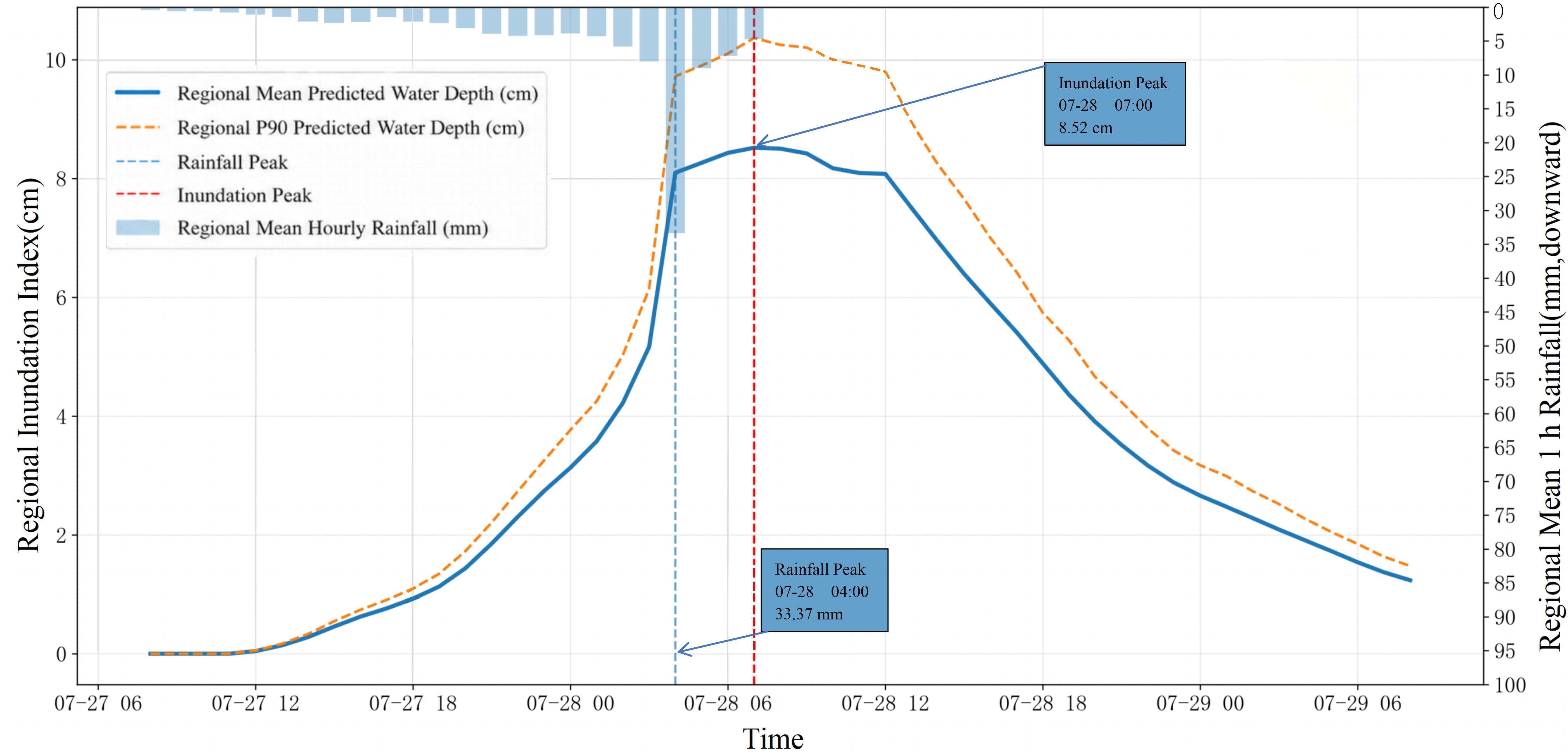
First, the regional mean inundation process did not respond synchronously to rainfall. It exhibited clear temporal accumulation and delayed response. The process followed a sequence of low-level stability, sustained rise, rapid increase, delayed peak, slow recession at a high level, and rapid recession. The inundation peak lagged behind the rainfall peak by about 3 h.

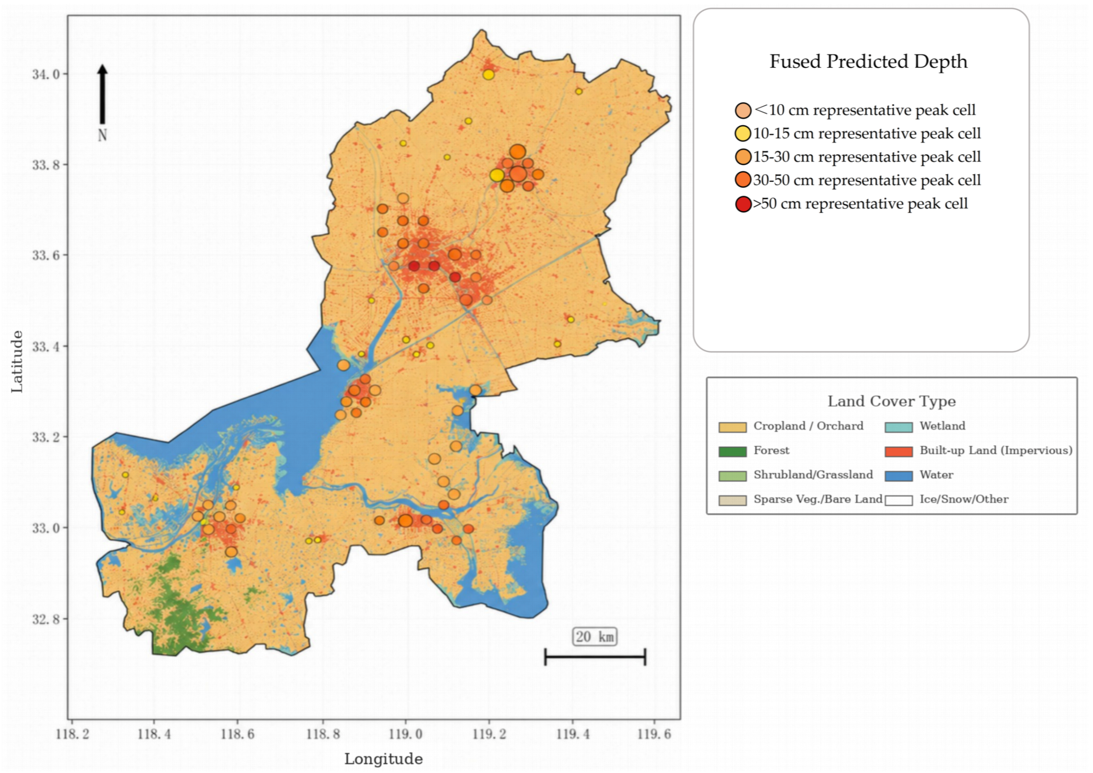
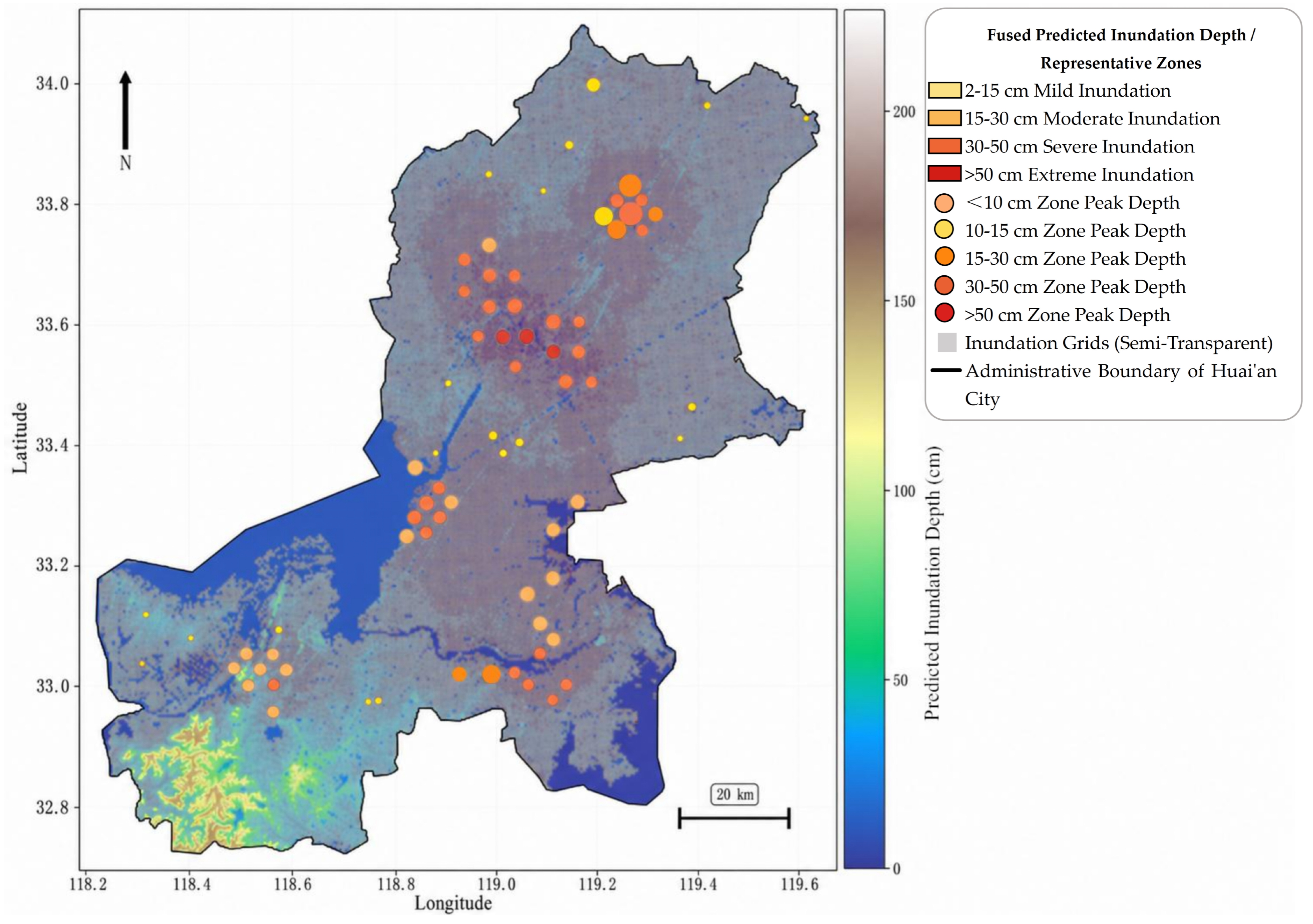
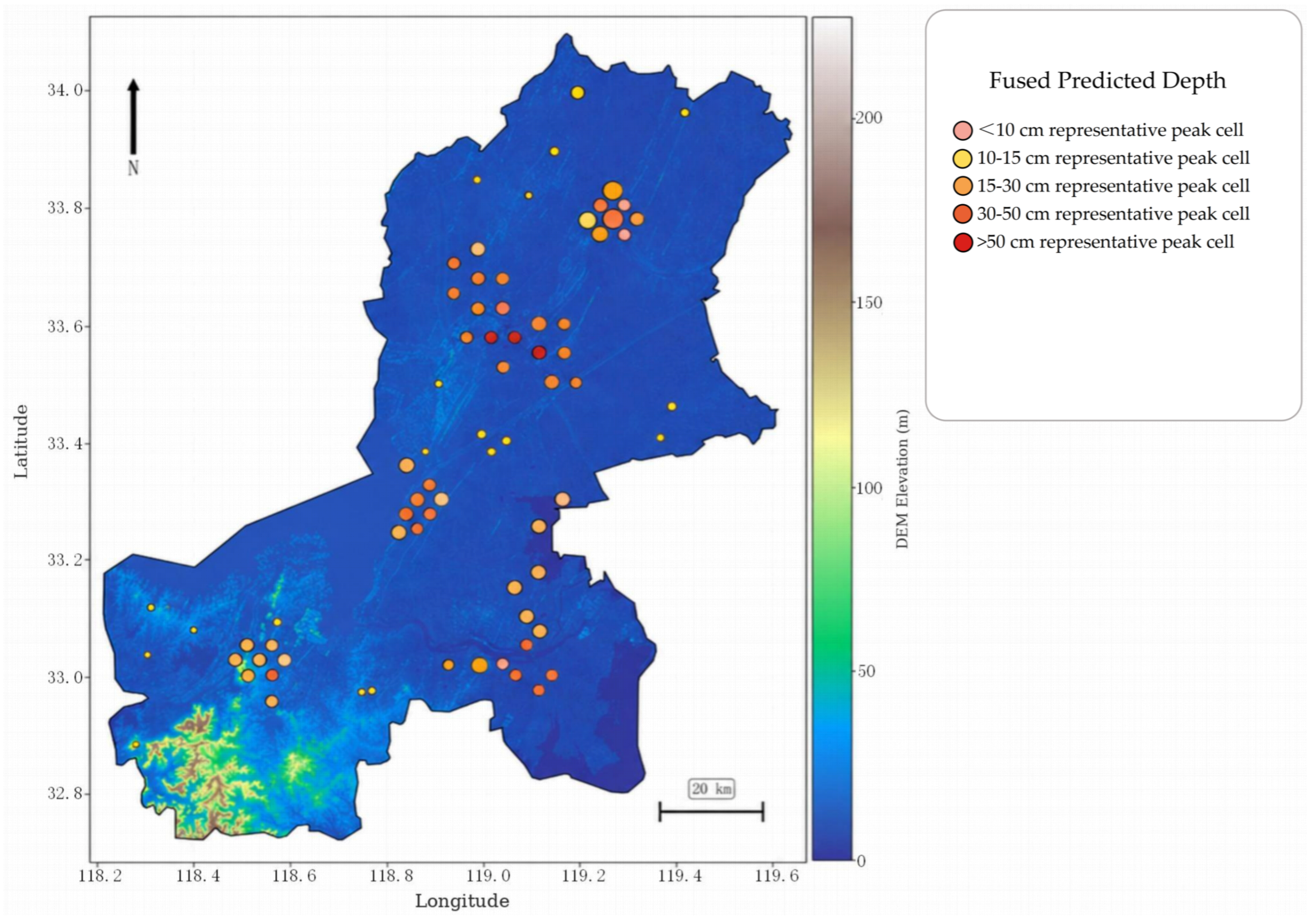
Second, high-inundation zones during the event exhibited pronounced spatial heterogeneity and inundation-level differentiation. The spatial pattern was characterized by concentration in the main urban built-up area, secondary distribution in county-level built-up areas, and scattered distribution in non-construction land. Mild and moderate inundation was more extensive, while medium-high and high-grade inundation was locally clustered.

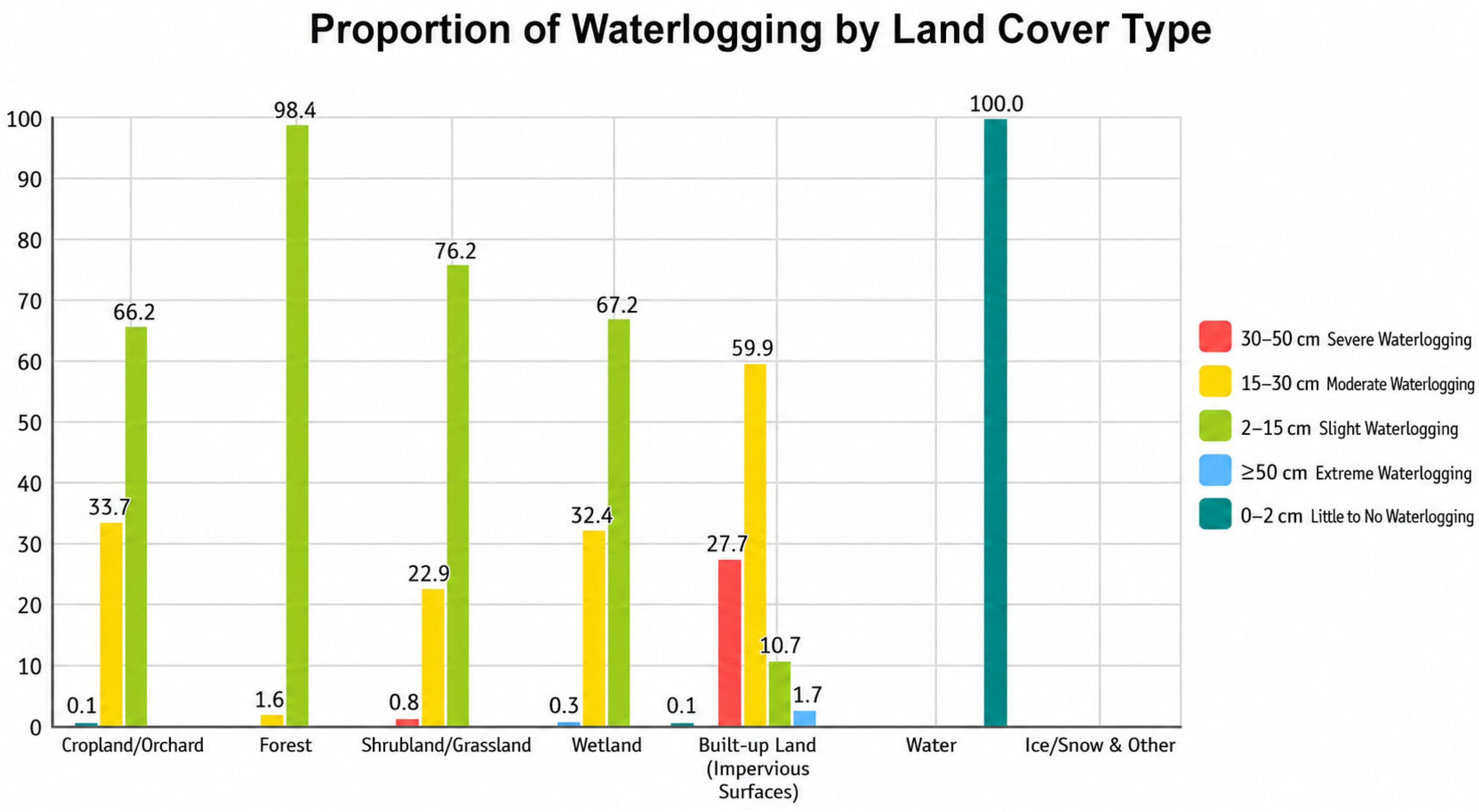
Third, the formation of high-inundation zones was controlled by multiple coupled factors. Low-lying terrain provided a physical basis for water retention. Impervious surfaces and built-up areas enhanced runoff generation and convergence. Drainage-network constraints and river-lake boundary conditions further affected discharge and persistence. Therefore, high-inundation zones cannot be explained by terrain or construction land alone.

Fourth, the proposed Transformer–GNN model effectively represents temporal dependencies and spatial structural constraints in urban-flood processes. Comparative experiments with LSTM, CNN, and U-Net demonstrated that the proposed framework achieved the highest prediction accuracy among all benchmark models. The model obtained an average R² of 0.9561, outperforming LSTM (0.7533), CNN (0.8232), and U-Net (0.9305), while simultaneously producing the lowest RMSE, MAE, and MAPE values. These results indicate that the fusion of Transformer-based temporal feature learning and graph neural network-based spatial topology representation provides a more effective characterization of urban flood-generation and propagation processes than conventional sequence-based or convolution-based deep-learning architectures. Therefore, the proposed framework can support event-scale inundation prediction, high-risk grid identification, and emergency decision-making with improved reliability.

Several limitations remain. First, because high-resolution observed inundation data are limited, training samples and validation results still partly depend on hydrodynamic simulations. Although the coupled SWMM–LISFLOOD-FP model provides physically consistent flood-depth information, uncertainties associated with rainfall inputs, parameter calibration, and drainage-network representation may influence the generated samples and consequently affect the performance of the data-driven prediction model. From an operational perspective, the uncertainty of the hydrodynamic simulations places an upper bound on the achievable accuracy of the Transformer–GNN surrogate model. The NSE value of 0.68 indicates that approximately 32% of the variance in observed inundation dynamics is not captured by the coupled SWMM-LISFLOOD-FP model. Consequently, part of this uncertainty is inevitably inherited by the simulation-generated training samples. However, the surrogate model is designed to learn the dominant spatiotemporal relationships between rainfall forcing, environmental characteristics, and inundation responses rather than reproducing local simulation noise. Therefore, the unexplained variance mainly affects prediction reliability in locations characterized by complex hydraulic interactions, drainage bottlenecks, or insufficient observational constraints. For city-scale flood forecasting and emergency management, the model is expected to provide robust identification of flood-prone areas, temporal flood evolution trends, and relative inundation severity. Nevertheless, local-scale water-depth predictions should be interpreted together with the uncertainty associated with the underlying hydrodynamic simulations. Future work will incorporate additional observed inundation records, real-time sensor measurements, and uncertainty-quantification techniques to further assess error propagation from hydrodynamic simulations to surrogate-model predictions and improve operational reliability.

Second, the analysis focuses on one representative heavy rainfall event and should be tested under more rainfall scenarios. Third, embedded uncertainty from rainfall input, drainage parameters, and model structure should be quantified more explicitly. Future work should integrate additional monitoring data, conduct multi-event validation, improve uncertainty analysis, and enhance interpretability of attention weights.

Overall, the Transformer–GNN fusion model offers a feasible approach for urban-flood prediction that integrates temporal-process representation and spatial-structure modeling. Future applications can connect this model with real-time rainfall forecasts, drainage-network operation data, and emergency dispatch platforms to support more dynamic urban flood-risk management.