Article

Physics-Consistent Overtopping Estimation for Dam-Break Induced Floods via AE-Enhanced CatBoost and TreeSHAP

1
Zhejiang Institute of Hydraulics & Estuary (Zhejiang Institute of Marine Planning & Design), Hangzhou 310020, China
2
School of Hydraulic Engineering, Zhejiang University of Water Resources and Electric Power, Hangzhou 310018, China
3
Zhejiang Key Laboratory of River-Lake Water Network Health Restoration, Hangzhou 310020, China
*
Author to whom correspondence should be addressed.
Water 2026, 18(1), 42; https://doi.org/10.3390/w18010042
Submission received: 24 November 2025 / Revised: 16 December 2025 / Accepted: 21 December 2025 / Published: 23 December 2025

Abstract

Dam break problem-induced floods can trigger hazardous dike overtopping, demanding predictions that are fast, accurate, and interpretable. We pursue two objectives: (i) introducing a new alpha evolution (AE) optimization scheme to improve tree-model predictive accuracy, and (ii) developing a cluster-wise modeling strategy in which regimes are defined by wave characteristics. Using a dataset generated via physical model experiments and smoothed particle hydrodynamics (SPH) numerical simulations, we first group samples via hierarchical clustering (HC) on the Froude number ( Fr ) , wave nonlinearity ( R ) , and relative distance to the dike ( D ) . We then benchmark CatBoost, XGBoost, and ExtraTrees within each cluster and select the best-performing CatBoost as the baseline, after which we train standard CatBoost and its AE-optimized variant. Under random train–test splits, AE-CatBoost achieves the strongest generalization for predicting relative run-up distance H m (testing dataset R 2 = 0.9803 , RMSE = 0.0599 ), outperforming particle swarm optimization (PSO) and grid search (GS)-tuned CatBoost. We further perform TreeSHAP analyses on AE-CatBoost for global, local, and interaction attributions. SHAP analysis yields physics-consistent explanations: D dominates, followed by H and L, with a weaker positive effect of Fr and minimal influence of R; H × D is the strongest interaction pair. Overall, AE optimization combined with HC-based cluster-wise modeling produces accurate, interpretable overtopping predictions and provides a practical route toward field deployment.

1. Introduction

Dam break problem-induced floods generate rapidly propagating bores that can drive extreme wave run-up and dike overtopping, posing acute risks to downstream communities and coastal defenses [1,2,3]. Accurate estimation of the maximum run-up distance is central to design and risk assessment: underestimation can precipitate catastrophic flooding and loss of life, whereas overly conservative allowances inflate construction and maintenance costs. In addition to accuracy alone, engineering practice increasingly requires physics-consistent predictions that not only fit the data but also align with governing hydrodynamics.
To predict the wave run-up and overtopping problems induced by propagation of single wave, studies have been conducted which involve theoretical models, laboratory experiments, computational fluid dynamic simulations, and field monitoring analysis [4,5,6]. Analytical theoretical solutions based on nonlinear shallow-water equations and Boussinesq-class models provide insight into dispersion and nonlinearity but rely on simplifying assumptions of bathymetry, wave form, etc. [7,8,9,10]. Empirical formulas offer practical tools yet remain valid only within tested ranges of wave nonlinearity, water depth, etc. [11,12,13,14,15]. Computational fluid dynamics simulations such as RANS and LES can resolve complicate fluid–structure interactions at the dike toe as well as aeration, but their computational expense confines them to more realistic case studies [16,17,18,19]. Field observations based on monitoring sensors have improved understanding of run-up processes, yet such datasets are always scenario-limited [20,21]. Hybrid models such as experimental–numerical and analytical–numerical combined models have also been explored [22,23,24,25].
With the development of computer science, recent studies have applied machine learning to develop prediction model such as neural networks, random forests, XGBoost, etc. [26,27,28,29,30,31]. Power et al. (2019) studied beach run-up using gene expression programming alongside empirical relationships [32]. Rehman et al. (2022) studied incident wave run-up using response-surface methodology coupled with neural networks [33]. Li et al. (2024) proposed a temporal convolutional neural network approach for run-up on a semi-submersible [34]. Naeini et al. (2024) proposed a physics-informed machine learning model for time-dependent wave-runup prediction [35]. Li et al. (2025) studied and compared LSTM and temporal convolutional network models for semisubmersible run-up [36]. These studies have advanced the state of machine learning for wave-runup problems, delivering notable gains in predictive accuracy while increasingly embedding or validating physical principles. However, most existing models do not explicitly account for heterogeneity across wave regimes, even though different wave characteristics can induce systematically different run-up responses. This omission may limit generalization and blur physical attributions.
Recent studies have increasingly incorporated clustering techniques into data-driven hydrodynamic modeling to account for regime-dependent behavior and to reduce data heterogeneity. Typical clustering-enhanced approaches first partition samples into distinct regimes based on selected physical or statistical features (e.g., wave characteristics or flow conditions), then train either separate predictive models for each cluster or a unified model augmented with regime information. Such strategies allow models to specialize across relatively homogeneous subspaces, and have been shown to improve predictive performance in wave run-up, dam break flows, and related hydraulic problems. For example, a very recent work by Li et al. (2025) introduced K-means clustering to account for wave-characteristic heterogeneity in run-up prediction [37]. While this work demonstrated the potential of clustering-based regime partitioning, it relied on a small-scale flume dataset, which limits similarity scaling and out-of-sample generalization. Moreover, the study did not conduct systematic model optimization or interpretability analyses, leaving open questions regarding robustness across regimes and the physical consistency of the learned relationships.
Motivated by these gaps, we introduce a cluster-wise strategy that partitions data by wave characteristics and then learns regime-specific predictors, with three key improvements: (i) we build upon a combined experimentally- and numerically-generated dataset to broaden similarity coverage and enhance generalizability; (ii) we benchmark tree learners and select the optimal model, then apply a novel optimization scheme to improve predictive accuracy; and (iii) we incorporate SHAP to provide physics-consistent global and local explanations clarifying how the wave parameters jointly shape overtopping outcomes.
This study advances physics-consistent overtopping estimation for dam break-induced flood overtopping via coupling hierarchical clustering (HC), alpha evolution (AE)-enhanced CatBoost, and TreeSHAP [38,39]. The dataset is generated via two dimensional physical model experiments and smoothed particle hydrodynamics (SPH) numerical simulations. First, we develop a cluster-wise modeling strategy in which regimes are defined by wave characteristics and cases are grouped via hierarchical clustering (HC) using the Froude number Fr , nonlinearity index R, and relative distance to the dike D as clustering criteria. Second, we benchmark three state-of-the-art tree learners—CatBoost, XGBoost, and ExtraTrees—and find that CatBoost outperforms the others, motivating its use as the baseline model. The target variable is the relative maximum run-up H m . Third, we introduce an alpha evolution (AE) optimization scheme that enhances CatBoost beyond particle swarm optimization (PSO) and grid search (GS), improving its predictive accuracy and stability. Fourth, to ensure physics consistency, we establish a TreeSHAP-based interpretability pipeline with the support of AE-Catboost to provide physics-consistent explanations at global, local, and interaction levels.
The rest of this paper is organized as follows. Section 2 describes the dataset, including the simplified physical model, the non-dimensional variables, and the physical model experiments and numerical simulations used to generate it. Section 3 presents the methodological framework, consisting of hierarchical clustering, CatBoost with the associated AE optimization, and the principles of TreeSHAP analysis. Section 4 reports the clustering results, the predictive performance of the proposed and baseline models, and SHAP-based interpretability analyses. Section 5 discusses the implications and methodological contributions of this study. Finally, Section 6 summarizes the key findings.

2. Dataset

2.1. Variables and Dimensionless Analysis

Figure 1 illustrates a two-dimensional simplified physical model of impulse-wave propagation toward a dike. Conceptually, the overall process can be divided into three stages. In a pre-stage (not modeled in this study), a dam break event in an upstream reservoir generates an impulse-like solitary wave. After the solitary wave has formed, Stage I (initial stage) describes its propagation over still water of uniform depth h 0 , characterized by wave height h w , wavelength l w , wave velocity u 0 , and an initial distance d between the wave front and the dike toe. Stage II (impacting stage) corresponds to the interaction between the wave and the dike, during which the free surface runs up along the slope and reaches a maximum elevation h m above the still-water level. The present work focuses on the post-dam break evolution; the dam break generation process itself is treated as a pre-stage that is outside the scope of the quantitative analysis. The objective is to predict the maximum run-up height h m on the dike from the impulse-wave characteristics ( h w , l w , u 0 , d , h 0 ) observed in the initial stage.
From the physical model in Figure 1, the maximum run-up height h m on the dike is governed by the incident-wave characteristics and the still-water depth. In dimensional form, this dependence can be written as
h m = f l w , u 0 , h w , d , h 0 , g ,
where l w is the incident wavelength, h w is the incident wave height, u 0 is the wave velocity at the wave crest, d is the initial distance from the wave front to the dike, h 0 is the still-water depth, and g is gravitational acceleration. The ratio of h w to l w provides a convenient measure of wave nonlinearity.
To collapse scale effects and expose the governing similarity parameters, we introduce the following dimensionless groups:
L = l w h 0 , Fr = u 0 g h 0 , D = d h 0
H = h w h 0 , R = H L = h w l w , H m = h m h 0
where L and H are the relative wavelength and wave height, Fr is the Froude number based on the still-water depth, D is the relative distance to the dike, R quantifies wave nonlinearity, and H m is the relative maximum run-up. Expressed in terms of these dimensionless variables, ( L , D , H , Fr , R ) serve as the basis for the subsequent data-driven modeling and interpretation.

2.2. Data Generation

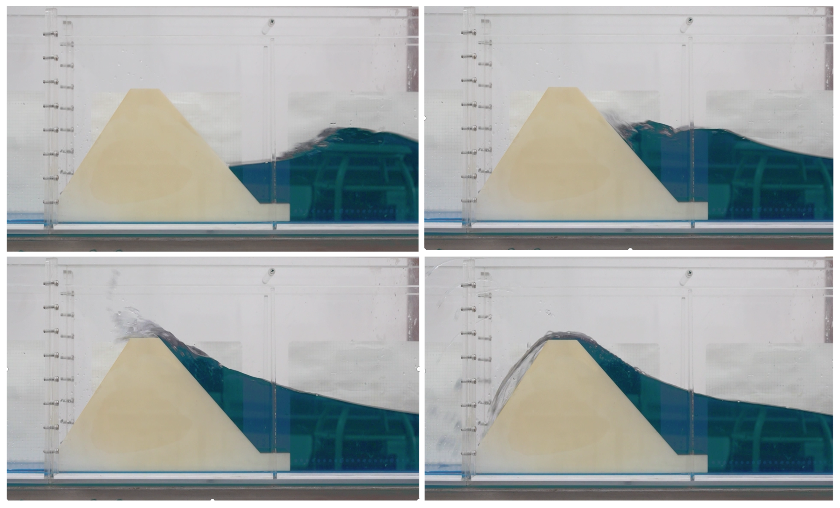
To build the dataset for model training, we combined small-scale physical model tests with companion numerical simulations. Figure 2 shows the sketch of the laboratory flume with a total length of 3 m and width of 0.2 m. The dam model is 30 cm wide at the base and 25 cm high. The slope is inclined at 45°. Figure 3 shows the impacting stage, where the dam break-induced impulse wave runs up and overtops the dike. Because the limited flume length restricts the range of incident wave conditions and propagation distances that can be realized experimentally, we complemented the experiments with numerical simulations using the same two-dimensional simplified configuration. The numerical model reproduces the dam break generation of an impulse wave, its subsequent propagation along the flume, and the overtopping of the dike. By extending the propagation distance and systematically varying the governing parameters, the simulations enrich the diversity of wave scenarios while remaining consistent with the physics observed in the experiments. Both the physical and numerical setups are based on the same two-dimensional simplified model of dam break-induced impulse wave propagation and overtopping. Compared with real-world coastal and reservoir geometries, this idealized layout omits detailed bathymetry and topographic complexity, which reduces the amount of information but allows us to focus on a controlled set of core variables and to perform systematic parameter variations. In total, 183 cases were generated from the combined physical and numerical dataset.
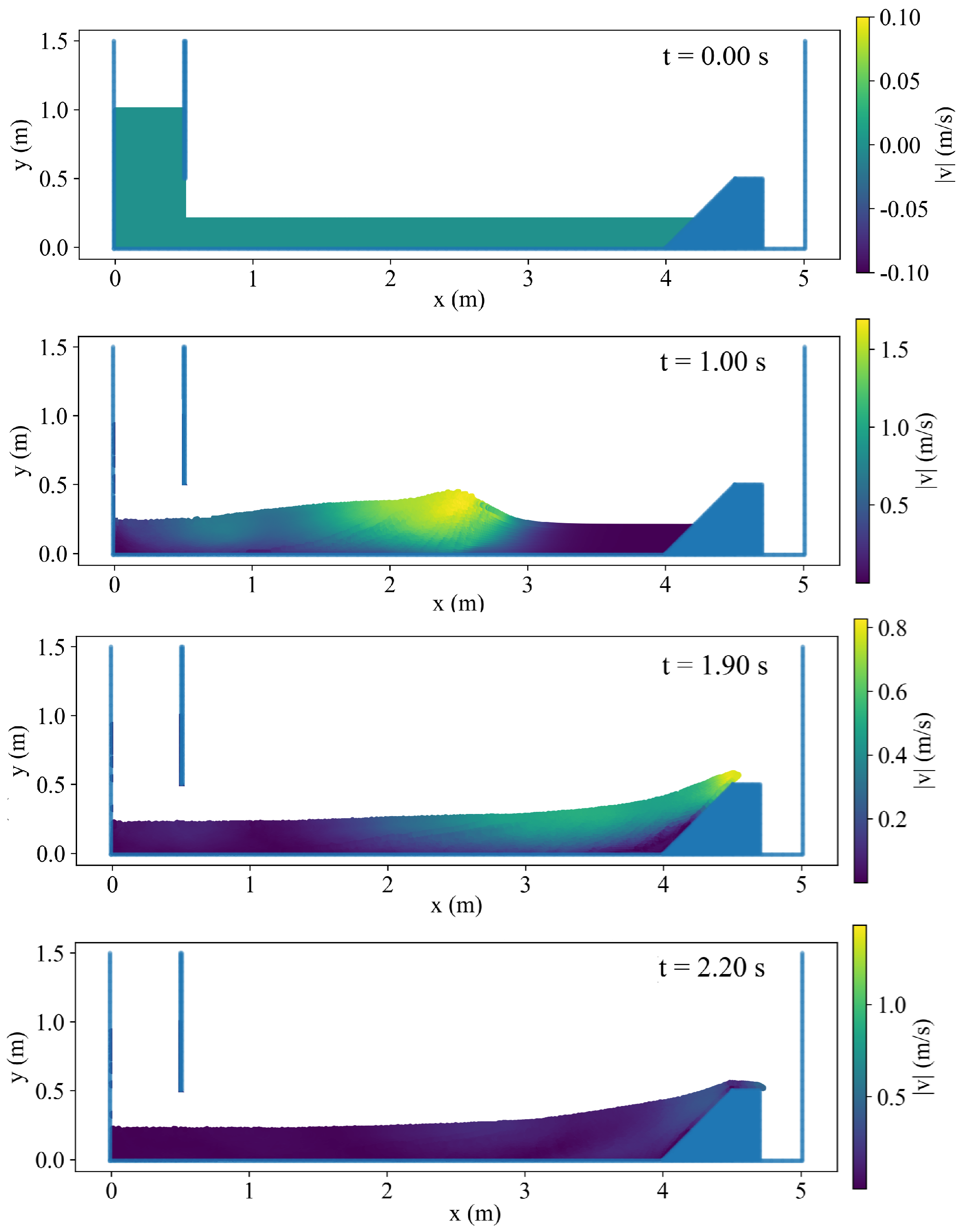
The smoothed particle hydrodynamics (SPH) method is adopted to perform the numerical simulations. Owing to its mesh-free and fully Lagrangian formulation, SPH is particularly well suited for modeling highly transient free-surface flows with large deformation, wave breaking, and strong fluid–structure interaction, which are characteristic of dam-break–induced impulse waves and dike overtopping. Based on the SPH simulations, Figure 4 illustrates the temporal evolution of the velocity magnitude during impulse wave propagation and overtopping, highlighting the key stages of wave development, impact, and energy dissipation.
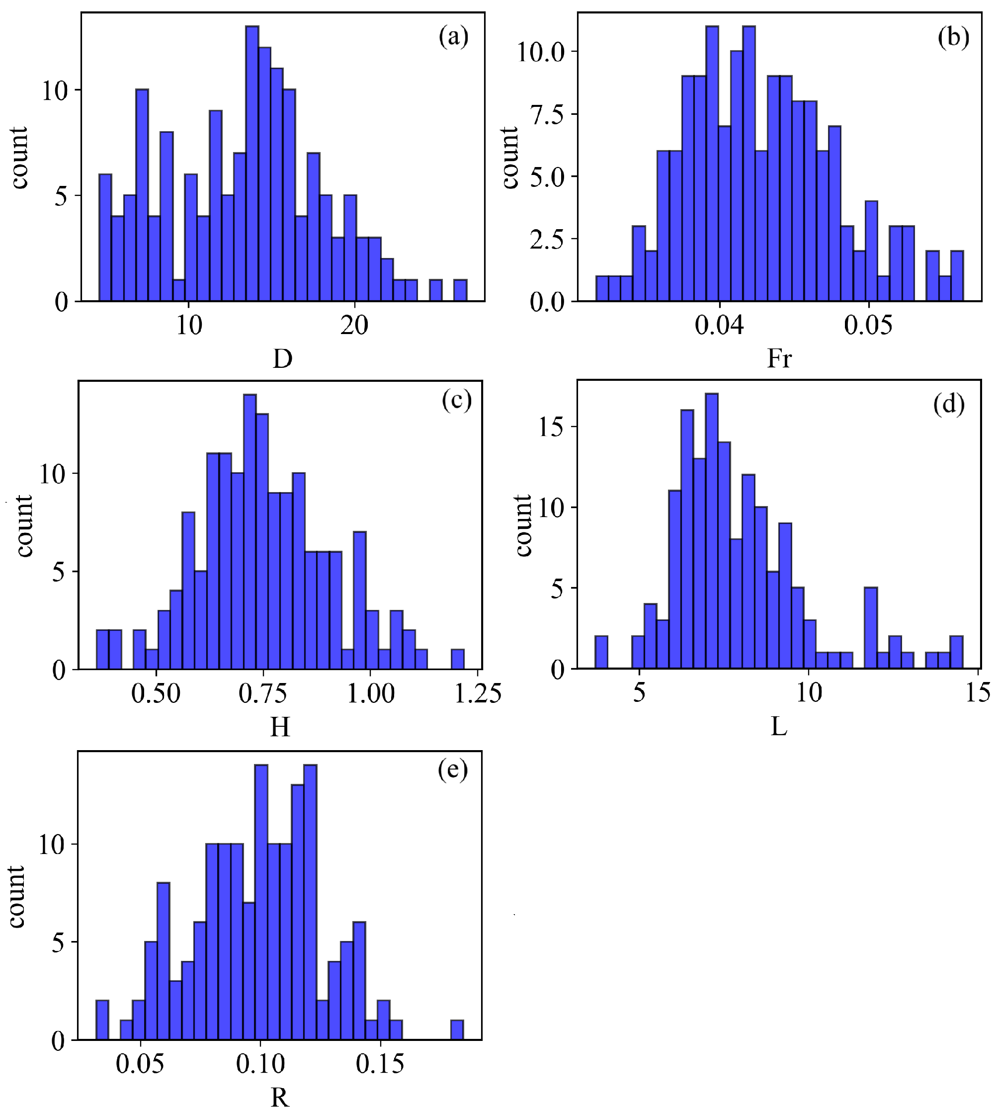
Figure 5 shows the histograms of the five dimensionless input variables for the 183 cases generated from physical model experiments and numerical simulations. All variables are approximately unimodal with limited skewness and no pronounced outliers. In specific, D concentrates around 5 to 20 with a mild right tail; Fr is tightly grouped in 0.035 to 0.055 with a peak near 0.04, consistent with a low-Froude regime; H lies mainly in 0.5 to 1.1 with a mode near 0.6 to 0.8; L covers from 5 to 12 and exhibits slight positive skew with a few larger wavelengths up to 15; and R centers at 0.07 to 0.11 with occasional cases as low as 0.05 and as high as 0.17. Overall, the sample provides broad yet balanced coverage of impulse wave conditions generated by dam break problem, supplying sufficient variability for learning the relation between the wave characteristics during propagation and over-topping on the sea dike.

3. Methods

3.1. Modeling Framework

In regression prediction and interpretability, combining tree models with SHAP is particularly advantageous. Tree-based learners flexibly capture nonlinear relations and higher-order interactions, while TreeSHAP provides exact, additively consistent Shapley attributions for ensembles, enabling quantitative explanations at both global and local levels.
Prior to model training, we clustered the dataset by wave characteristics using a hierarchical clustering method to stratify wave regimes, reduce heterogeneity, and enable stratified evaluation and subgroup-wise interpretation. We then compared three tree models that have proven strong in recent studies—CatBoost, XGBoost, and ExtraTrees—and selected CatBoost as the baseline based on its superior test-set performance in terms of R 2 and RMSE. Next, to further improve accuracy, we applied an alpha evolution (AE) scheme for hyperparameter optimization and contrasted AE-CatBoost with PSO-CatBoost, GS-CatBoost, and an unoptimized CatBoost. The results show that AE-CatBoost delivers gains in both accuracy and stability, confirming the effectiveness of AE for hyperparameter tuning. Building upon the selected predictive model, we constructed a TreeSHAP analysis framework to systematically assess the marginal contributions and interaction effects of the inputs D , Fr , H , L , R on the output H m .
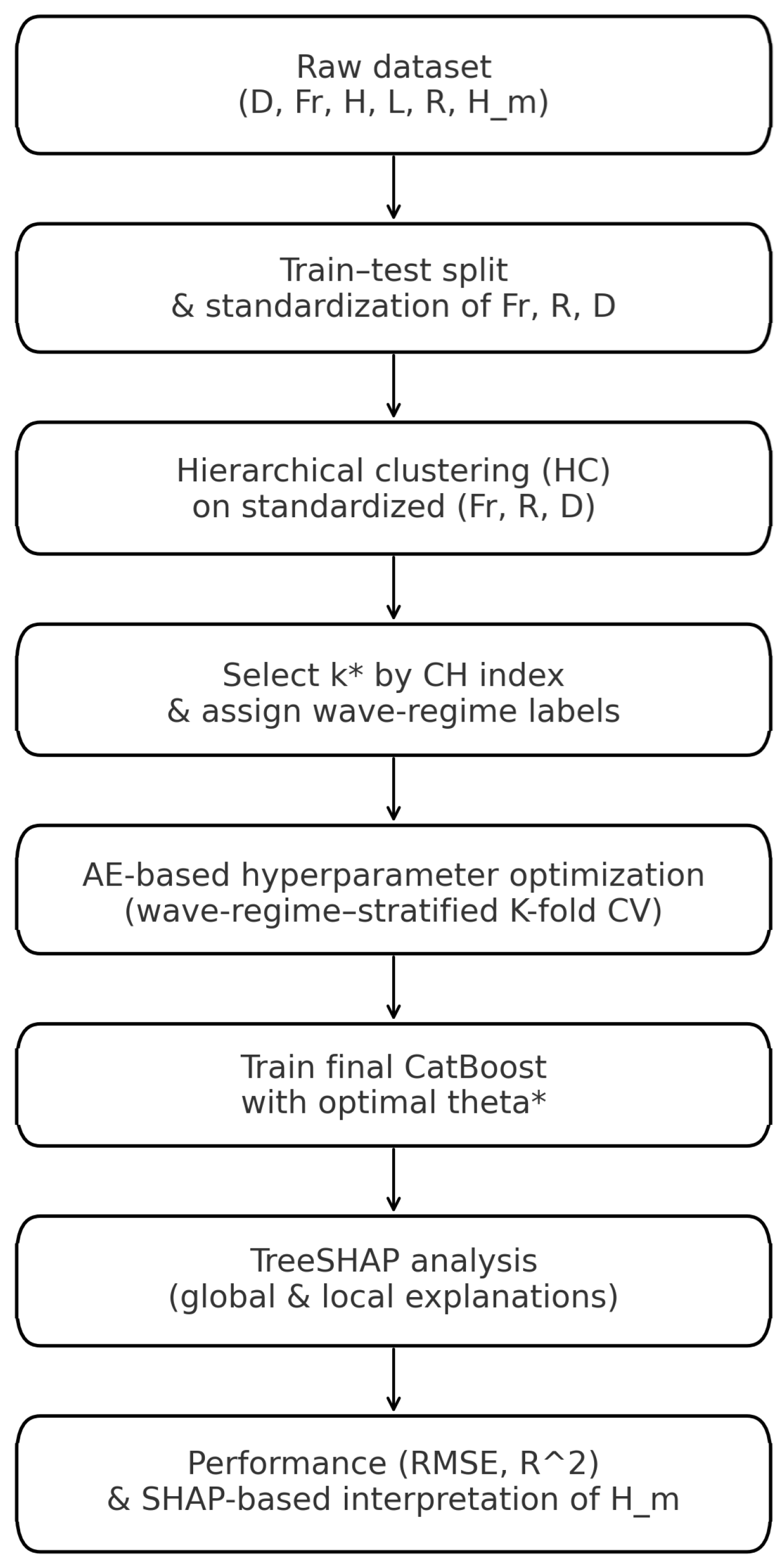
In Figure 6, we present the mathematical underpinnings of the hierarchical clustering (HC), the chosen CatBoost tree model, the alpha evolution (AE) optimization scheme, and the TreeSHAP analysis. The pseudocode is provided in Appendix A.

3.2. Hierarchical Clustering

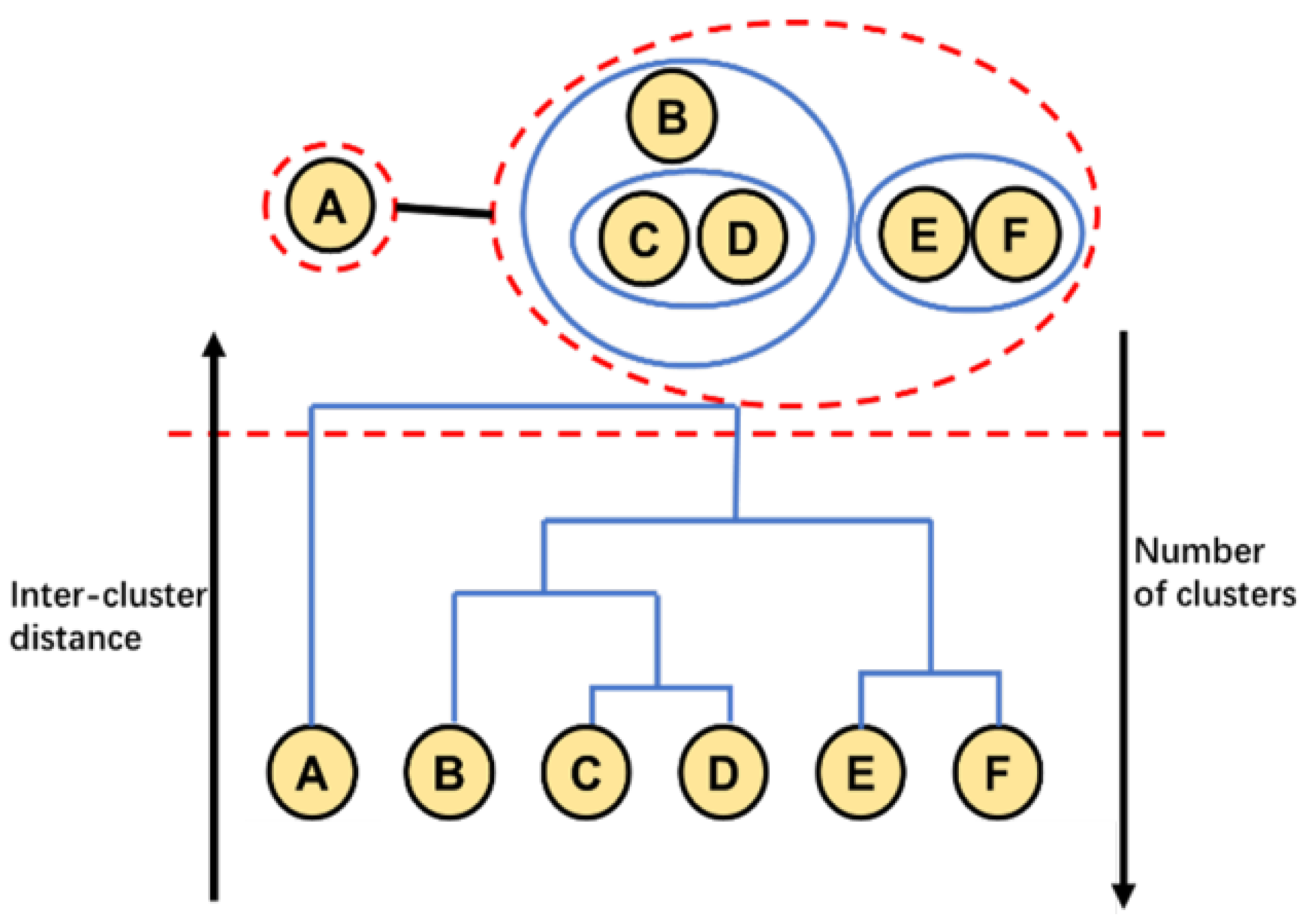
We stratify the data by wave characteristics via agglomerative hierarchical clustering (HC) on three features ( Fr , R , D )  [40,41,42]. Figure 7 illustrates the principle of the hierarchical clustering (HC) method.
To remove scale effects, each feature is standardized using statistics computed on the training set to avoid leakage. For sample i,
z i j = x i j μ j σ j , j { Fr , R , D } ,
yielding z i = [ z i , Fr , z i , R , z i , D ] R 3 . The Euclidean distance is used in the standardized space.
We adopt agglomerative clustering with Ward linkage. Starting from singletons, at each step we merge the pair of clusters that produces the smallest increase in within-cluster sum of squares (WSS). Let C = { C 1 , , C k } denote the current partition, with centroids z ¯ C . The within-cluster dispersion is
WSS ( C ) = C C z i C z i z ¯ C 2 2 .
Ward linkage selects the merge that minimizes the increment Δ WSS ; equivalently, it minimizes the increase in total error sum of squares at each agglomeration step.
To determine the number of clusters, we cut the dendrogram at k that maximizes the Calinski–Harabasz (CH) index over a candidate range (e.g., k = 2 , , 6 ). Define the total sum of squares
TSS = i = 1 n z i z ¯ 2 2 , BSS ( k ) = TSS WSS ( C k ) ,
where z ¯ is the global mean and C k is the k-cluster partition. The CH index is
CH ( k ) = BSS ( k ) / ( k 1 ) WSS ( C k ) / ( n k ) .
We set k = arg max k CH ( k ) and use the resulting labels for downstream modeling.

3.3. CatBoost Prediction

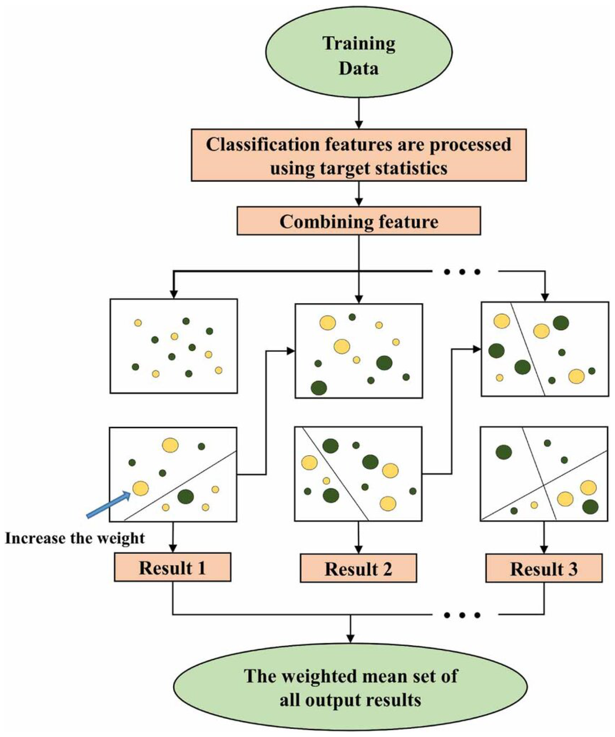
This study employs CatBoost (Categorical Boosting) to construct a regression model for H m  [43]. See Figure 8 for the principle of CatBoost algorithm.
Let the input vector be x = ( D , Fr , H , L , R ) and the response be H m . CatBoost is an additive model based on gradient boosting. After M trees, the prediction is
H ^ m ( x ) = F M ( x ) = m = 1 M η m T m ( x ) .
Here, η m ( 0 , 1 ] is the learning rate and T m ( · ) is the m-th base learner. A depth-d symmetric tree contains 2 d leaves, each with a constant value. To minimize empirical risk, this study adopts the squared error loss
L = i = 1 N H m , i F ( x i ) 2 .
At iteration m, CatBoost fits the negative gradient of the previous model. Denote the first- and second-order derivatives for sample i as
g i ( m ) = L F F = F m 1 ( x i ) ,
h i ( m ) = 2 L F 2 F = F m 1 ( x i ) ;
then, the output of each leaf of the m-th tree is updated by a Newton-like step
v = i g i ( m ) i h i ( m ) + λ ,
where λ > 0 is an 2 regularization term on leaf values. Under squared error, g i ( m ) = F m 1 ( x i ) H m , i and h i ( m ) = 1 . Hyperparameters (tree depth d, number of boosting iterations M, learning rate η , regularization λ , etc.) are selected via alpha evolution (AE) optimization. The primary metrics are root mean squared error (RMSE) and coefficient of determination R 2 .

3.4. Alpha Evolution Optimization

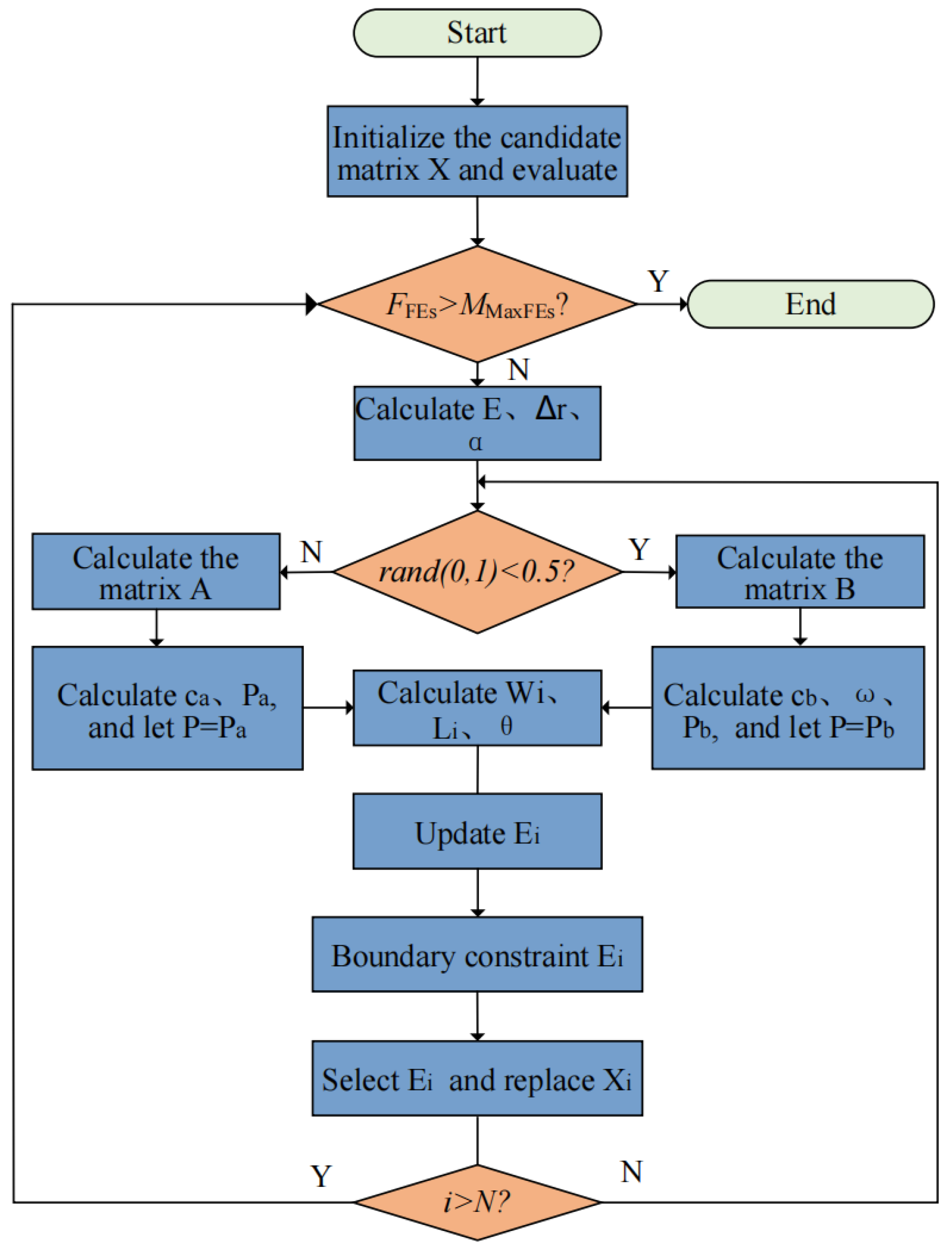
To obtain a high-accuracy and stable predictor for H m from inputs D , Fr , H , L , R , we optimize CatBoost hyperparameters with an efficient evolutionary scheme termed alpha evolution (AE) [44]. Alpha evolution (AE) integrates domain-scaled exploration, adaptive evolution paths, and elite–non-elite contrastive guidance, enabling efficient global search while maintaining stable convergence. Unlike surrogate-based Bayesian optimization or covariance matrix-based strategies, AE avoids strong distributional assumptions and high computational overhead, making it particularly suitable for the mixed and nonlinear hyperparameter space of CatBoost. See Figure 9 for the flowchart of AE optimization.
The decision vector is hyperparameters of CatBoost:
θ = ( d , M , η , λ ) .
AE solves a bounded minimization of the cross-validated RMSE:
min θ [ lb , ub ] f ( θ ) s . t . f ( θ ) = RMSE CV ,
where K-fold CV is stratified by the hierarchical-clustering wave regimes; early stopping is applied within each fold.
A population X R N × d (row X i is individual i) is initialized uniformly:
X i j U ( lb j , ub j ) , FEs FEs + N .
At each generation, evaluate f ( X i ) , set E X , and sort indices ind = argsort f ( X ) . Domain-scaled exploratory steps are
Δ r = ( ub lb ) 2 R 1 R 2 R 2 S , R 1 , R 2 U ( 0 , 1 ) N × d , S Bernoulli ( 0.5 ) N × d ,
and the progress factor is
α = exp ln 1 FEs MaxFEs 4 FEs MaxFEs 2 .
A global reference P R d is formed by reweighted subpopulation aggregation. Let K = N rand ( ) , draw I 1 = randperm ( N , K ) , set B = X ( I 1 , : ) , choose nonnegative ω with 1 ω = 1 , and define
c a = 1 FEs / MaxFEs , P c a P + ( 1 c a ) j = 1 K ω j B j : .
For contrastive guidance, pick u from the elite half of ind and v from the remainder, set W i = X u , L i = X v , and draw a perturbation weight
ϑ i = I 2 1 d · rand ( 0 , 2 ) + ( 1 I 2 ) rand ( 0 , 1 ) 1 × d
with I 2 Bernoulli ( 0.5 ) . Then, update individual i by
E i t + 1 = P + α Δ r i + ϑ i W i + E i t P L i .
Apply bounded handling and greedy selection:
E i t + 1 = min max { E i t + 1 , lb } , ub ,
X i t + 1 = E i t + 1 , f ( E i t + 1 ) f ( X i t ) , X i t , otherwise .
Increase FEs accordingly and stop when FEs MaxFEs . The best θ is then used to train the final CatBoost model for predicting H m from ( D , Fr , H , L , R ) .

3.5. TreeSHAP Analysis

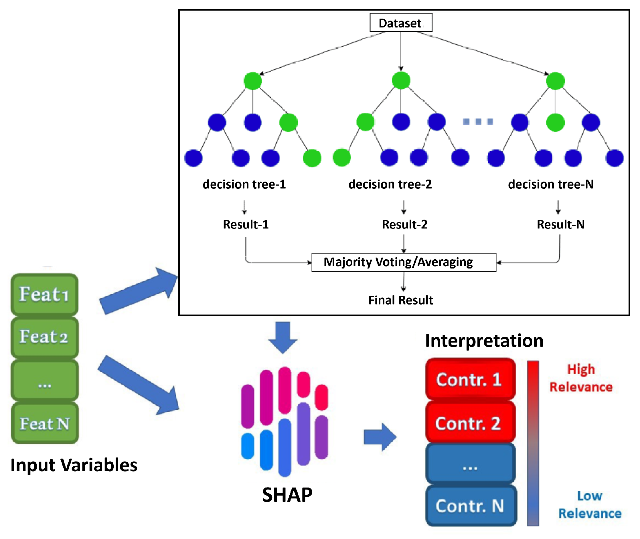
To quantify the marginal contributions of inputs to H ^ m , this study employs TreeSHAP based on Shapley values [45,46,47]. Figure 10 illustrates the principle of integrating tree models and SHAP analysis.
For any sample x , the prediction decomposes as
F ( x ) = ϕ 0 + j = 1 5 ϕ j ( x ) ,
where ϕ 0 = E [ F ( X ) ] is the baseline output (global expectation) and ϕ j ( x ) denotes the contribution of feature j { D , Fr , H , L , R } at x , satisfying the additivity property. TreeSHAP provides exact and efficient Shapley computations for tree models. Global importance is measured by the sample average of absolute SHAP values:
I j = E x | ϕ j ( x ) | ,
which yields an ordering of D , Fr , H , L , R by their average impact on H m . Local interpretation uses the set { ϕ j ( x ) } for a single sample to explain how its prediction deviates from  ϕ 0 .

4. Results

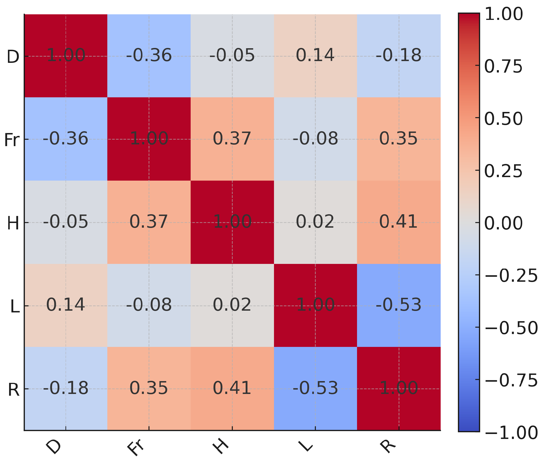
Figure 11 illustrates the Pearson correlation heatmap of the five input variables ( D , Fr , H , L , R ). Overall, pairwise correlations are modest. The largest absolute value is between L and R ( r = 0.53 ), which remains below a common collinearity threshold (<0.6); hence, all five variables are retained as predictors. The relatively higher LR association is physically reasonable: R characterizes wave nonlinearity and L reflects wavelength, which are inherently related. Nevertheless, it is useful to distinguish nonlinearity from amplitude- and length-related parameters, because wave type can alter propagation and run-up. Given the correlation is still moderate (<0.6), R is kept in the model.

4.1. Clustering Results

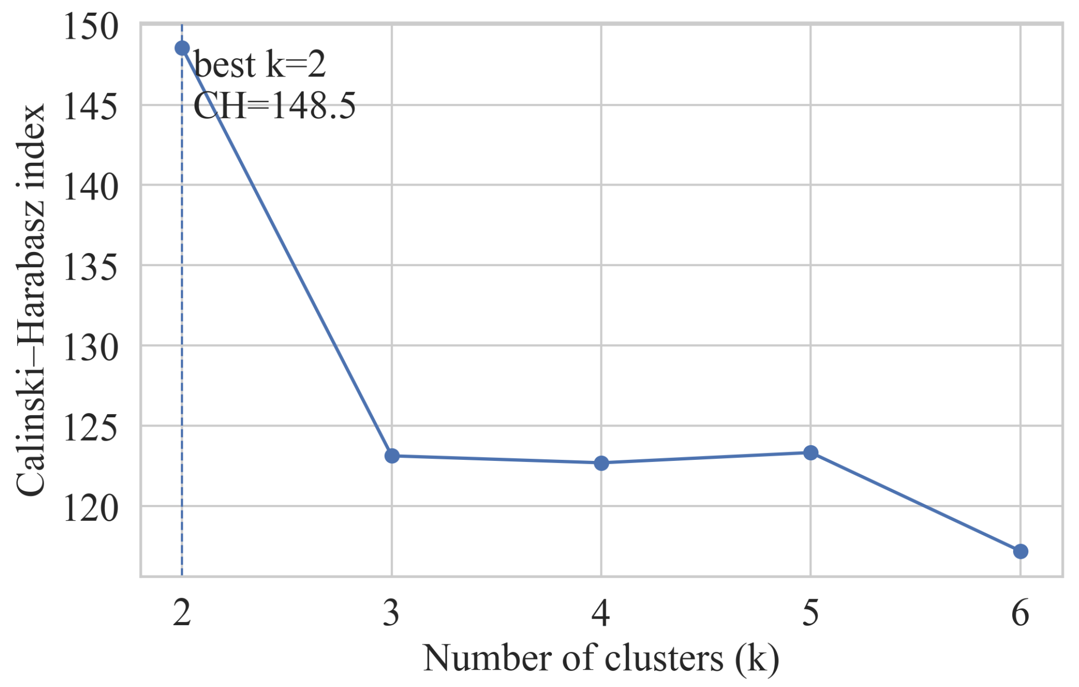
Figure 12 illustrates the Calinski–Harabasz (CH) index across candidate cluster counts k { 2 , 3 , 4 , 5 , 6 } . The index attains its global maximum at k = 2 with CH = 148.5 ; for k = 3 –6, CH ( k ) [ 118 , 123 ] , which is clearly below the two-cluster solution, yielding k = 2 . Physically, this aligns with two regimes: a nearshore, more nonlinear, and higher-Froude regime (small D, large R, higher Fr ) favoring larger H m , and an offshore, weaker-nonlinearity, lower-Froude regime (large D, small R, lower Fr ) that tends to suppress H m .
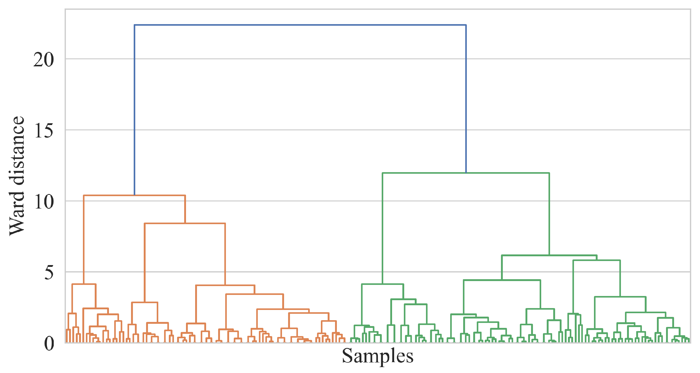
Figure 13 shows the Ward-linkage dendrogram. The two main clusters merge only at a Ward distance of 22, whereas most within-branch merges occur at area smaller than 12, indicating much larger inter-cluster than intra-cluster costs and a stable two-cluster structure. Interpreted by variable meaning, one branch aggregates cases with small D, large R, and higher Fr (energy/nonlinearity-driven uprush, larger H m ), while the other gathers large D, small R, and lower Fr (dissipation-dominated mild conditions, smaller H m ).
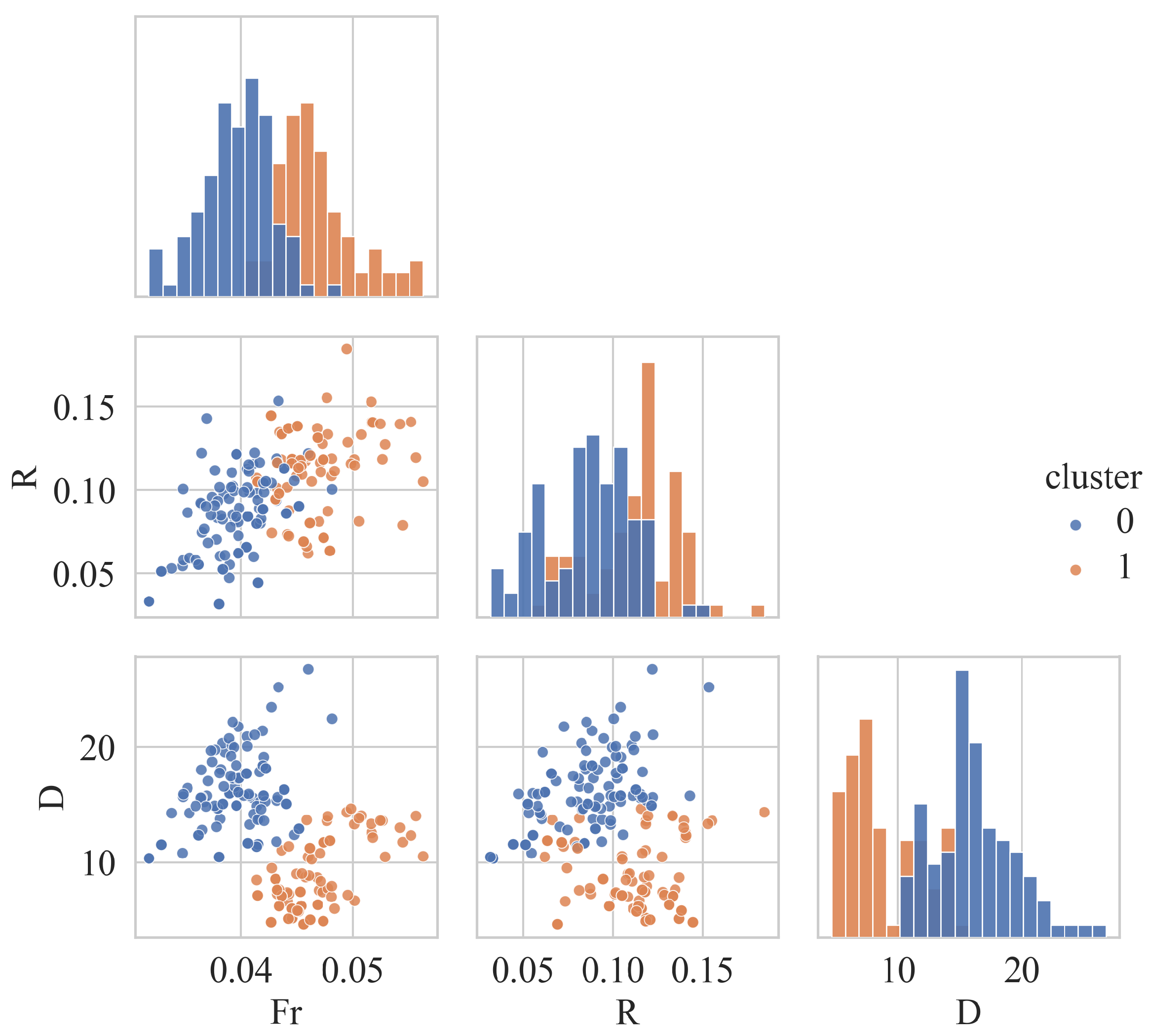
Figure 14 shows the pairwise scatter plots and marginal histograms in ( Fr , R , D ) space. Cluster 0 (blue) concentrates in D [ 12 , 22 ] , R [ 0.07 , 0.11 ] , Fr [ 0.035 , 0.045 ] (offshore, weakly nonlinear, low-Froude); Cluster 1 (orange) concentrates in D [ 6 , 14 ] , R [ 0.10 , 0.15 ] , Fr [ 0.045 , 0.055 ] (nearshore, more nonlinear, higher-Froude). Overlap is confined to a narrow band R between 0.10 and 0.11, D between 12 and 14, and Fr between 0.04 and 0.06, marking transitional cases. Larger H and higher Fr increase specific energy and momentum flux, larger R strengthens bore-like fronts, and larger D increases dissipation; the observed structure matches the expected effects on H m . Given the moderate LR correlation ( r = 0.53 < 0.6 ), both are retained to disentangle wavelength- versus nonlinearity-driven mechanisms.
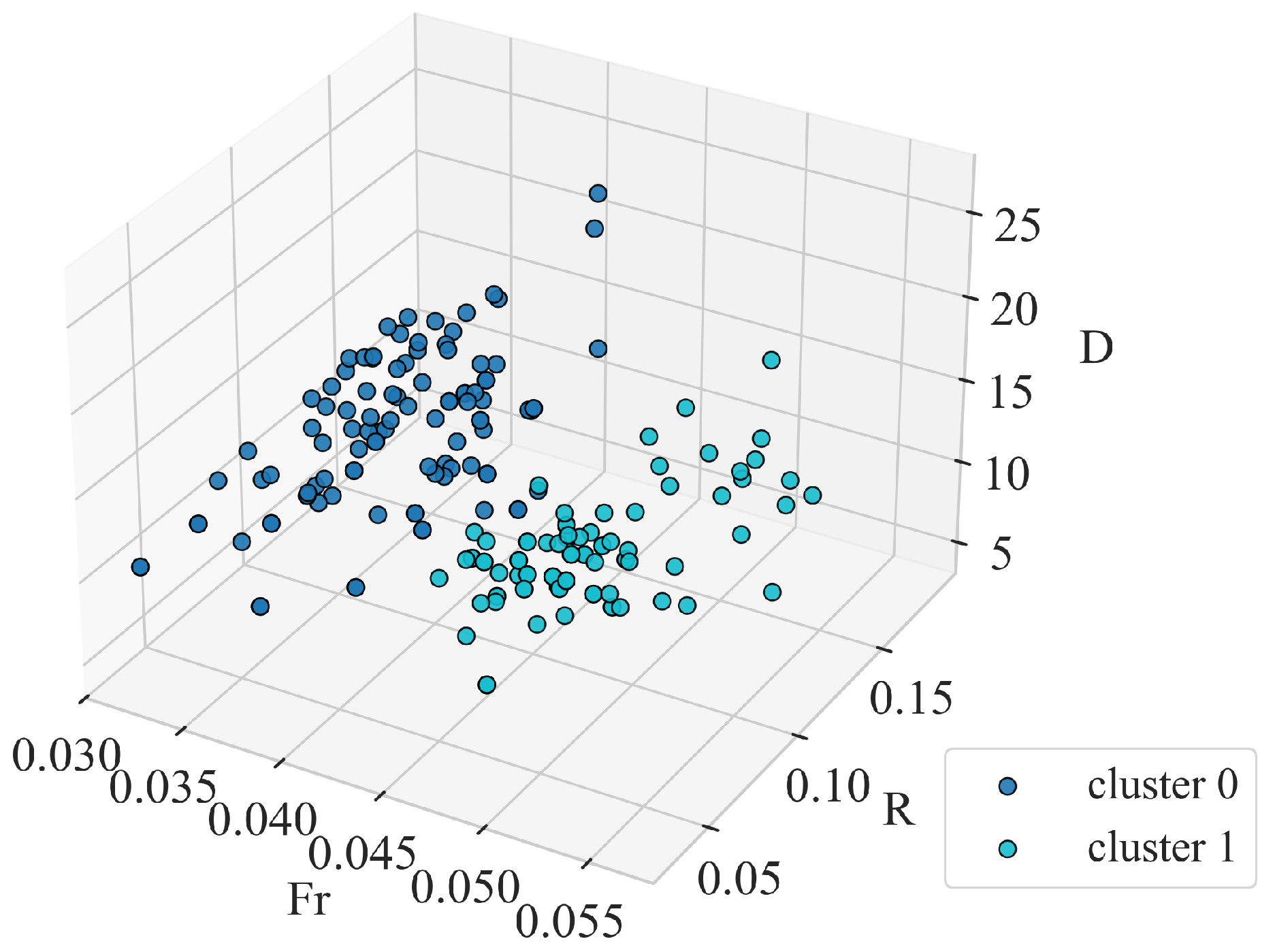
Figure 15 is the 3D scatter in ( Fr , R , D ) showing voxel-level separation. Cluster 0 occupies D 12 , R 0.11 , Fr 0.045 ; Cluster 1 concentrates in D 14 , R 0.10 , Fr 0.045 , intersecting only near R = 0.10 0.11 and D = 12 –14. This geometry suggests that in the low-D–high-R–high- Fr volume, TreeSHAP will yield positive contributions to H m , whereas high-D regions will show negative contributions ( ϕ D < 0 ); the effect of L is typically nonlinear or thresholded, with potential saturation at extreme values. Overall, the 3D separation is consistent with Figure 9, Figure 10 and Figure 11 and supports cluster-stratified validation and interpretation.

4.2. Prediction Results

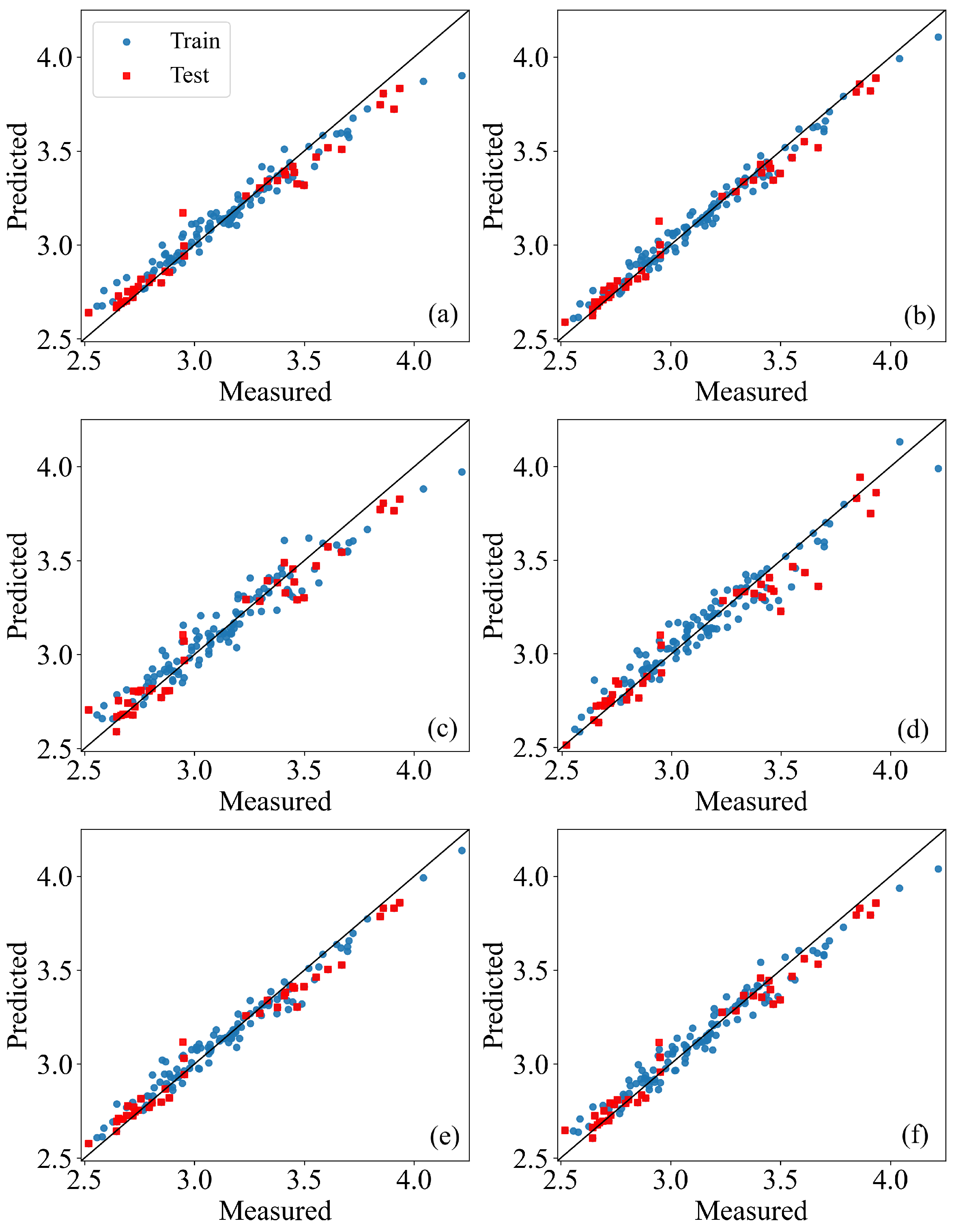
We adopt an 80/20 chronological split: we train on 80% of observations and hold out the left 20% as testing data. Figure 16 shows scatter plots of measured versus predicted values for the six models on the training and test sets. We first evaluated three tree-based baselines—CatBoost, XGBoost, and ExtraTrees—and found that CatBoost performed best ( R 2 = 0.9639 , RMSE = 0.0810 for the testing dataset). Using CatBoost as the baseline, we then applied two optimization strategies: AE-CatBoost as the proposed model, with PSO-CatBoost and GS-CatBoost as validation models. Across panels, most points cluster near the 1:1 line. AE-CatBoost exhibits the tightest cloud with the smallest deviations, indicating the strongest fit and generalization. PSO-CatBoost and GS-CatBoost follow, while XGBoost and ExtraTrees show greater dispersion. To further highlight the performance gain, Figure 16 should be interpreted in conjunction with the evaluation metrics in Figure 17 and residual distributions shown in Figure 18. While the scatter plots provide a qualitative comparison across models, the residual histograms and KDE curves offer a clearer quantitative contrast between the baseline CatBoost and AE-CatBoost.
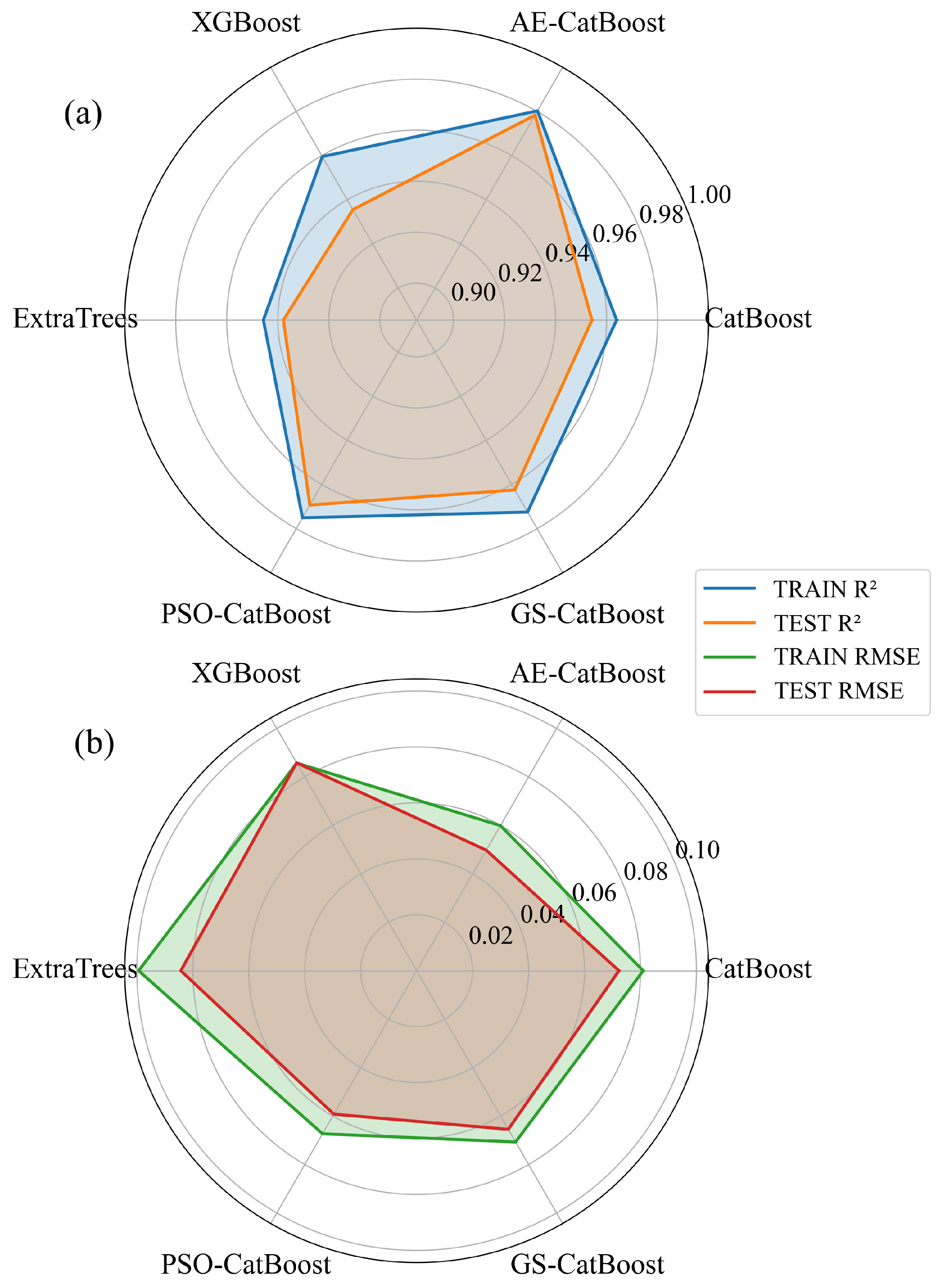
Figure 17 shows radar plots comparing R 2 and RMSE across all models. AE-CatBoost sits closest to the outer ring on R 2 and the inner ring on RMSE , achieving train/test R 2 = 0.9783 / 0.9803 and RMSE = 0.0498 / 0.0599 . Relative to the CatBoost baseline (test R 2 = 0.9639 , RMSE = 0.0810 ), AE-CatBoost increases test R 2 by + 0.0164 and reduces test RMSE by 0.0211 (26% reduction), and also lowers the test residual variance from 0.00652 to 0.00360 (45% reduction). PSO-CatBoost ranks second with test R 2 = 0.9751 and RMSE = 0.0673 , representing a 17% error reduction versus the baseline. GS-CatBoost follows closely at R 2 = 0.9725 and RMSE = 0.0707 (13% reduction). In contrast, XGBoost ( R 2 = 0.9596 , RMSE = 0.0857 ) and ExtraTrees ( R 2 = 0.9457 , RMSE = 0.0994 ) trail behind; AE-CatBoost cuts test error by roughly 30% and 40% compared with these two models, respectively. The small train–test gaps for AE-CatBoost further indicate stable generalization rather than overfitting. Overall, CatBoost outperforms XGBoost and ExtraTrees among the baselines, and the AE enhancement yields a clear and quantitatively larger gain than either PSO or grid search.
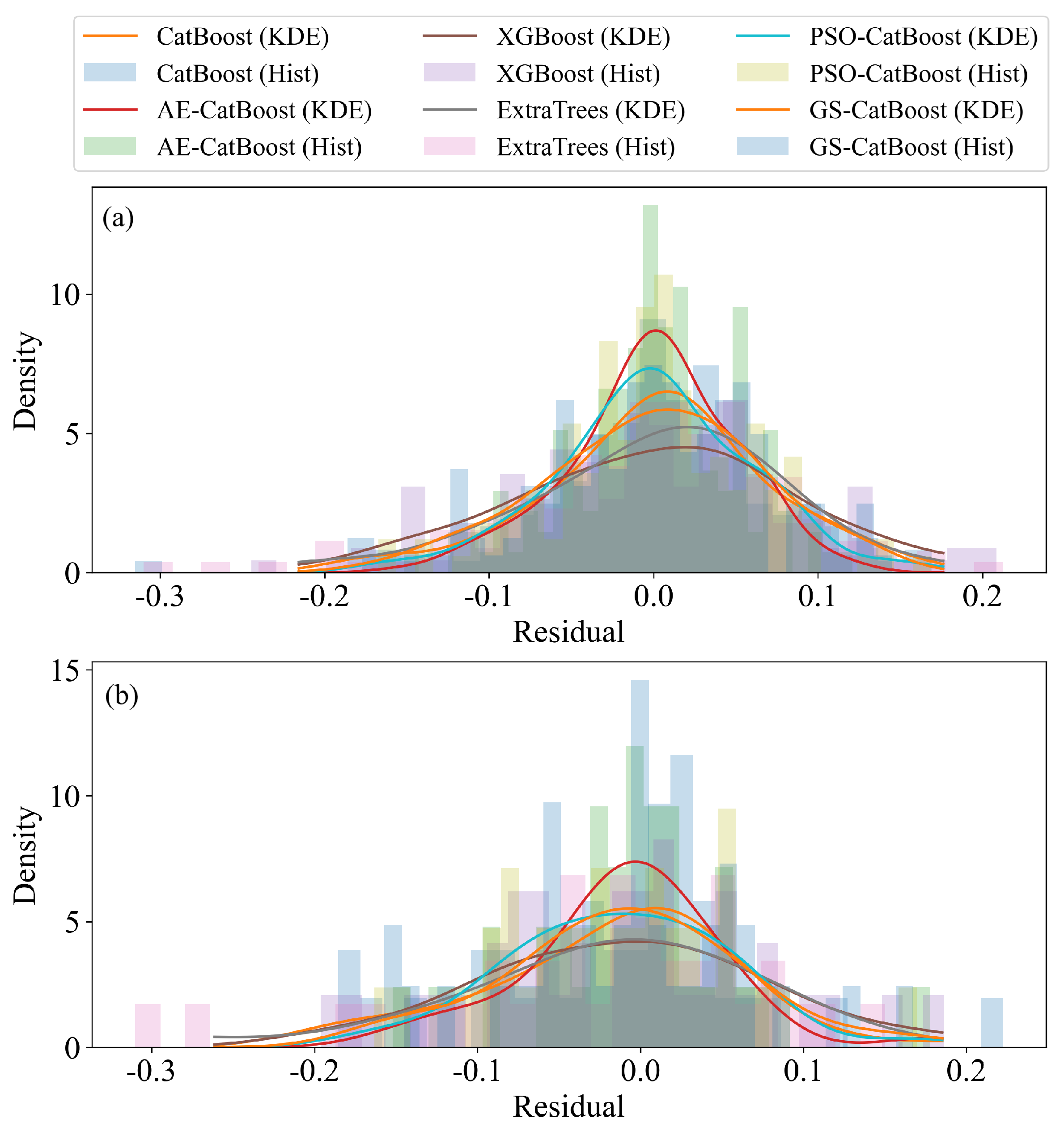
Figure 18 shows histograms and kernel density estimates of residuals for the training and test sets. The bars show normalized histograms and the solid curves are kernel density estimates (KDEs). Here, the KDE is a non-parametric estimator of the probability density function. It places a smooth kernel at each residual and sums them to produce a continuous density curve. Here, residuals are centered around zero and are approximately Gaussian with no obvious systematic bias. AE-CatBoost displays the sharpest peak, the narrowest spread, and the shortest tails, reflecting the lowest variance and the most stable errors. PSO-CatBoost and GS-CatBoost are next and the baseline CatBoost follows, with XGBoost and ExtraTrees exhibiting wider spreads and heavier tails. These residual patterns corroborate the quantitative results from Figure 14 and further confirm AE-CatBoost as the best-performing model.

4.3. TreeSHAP Analysis Results

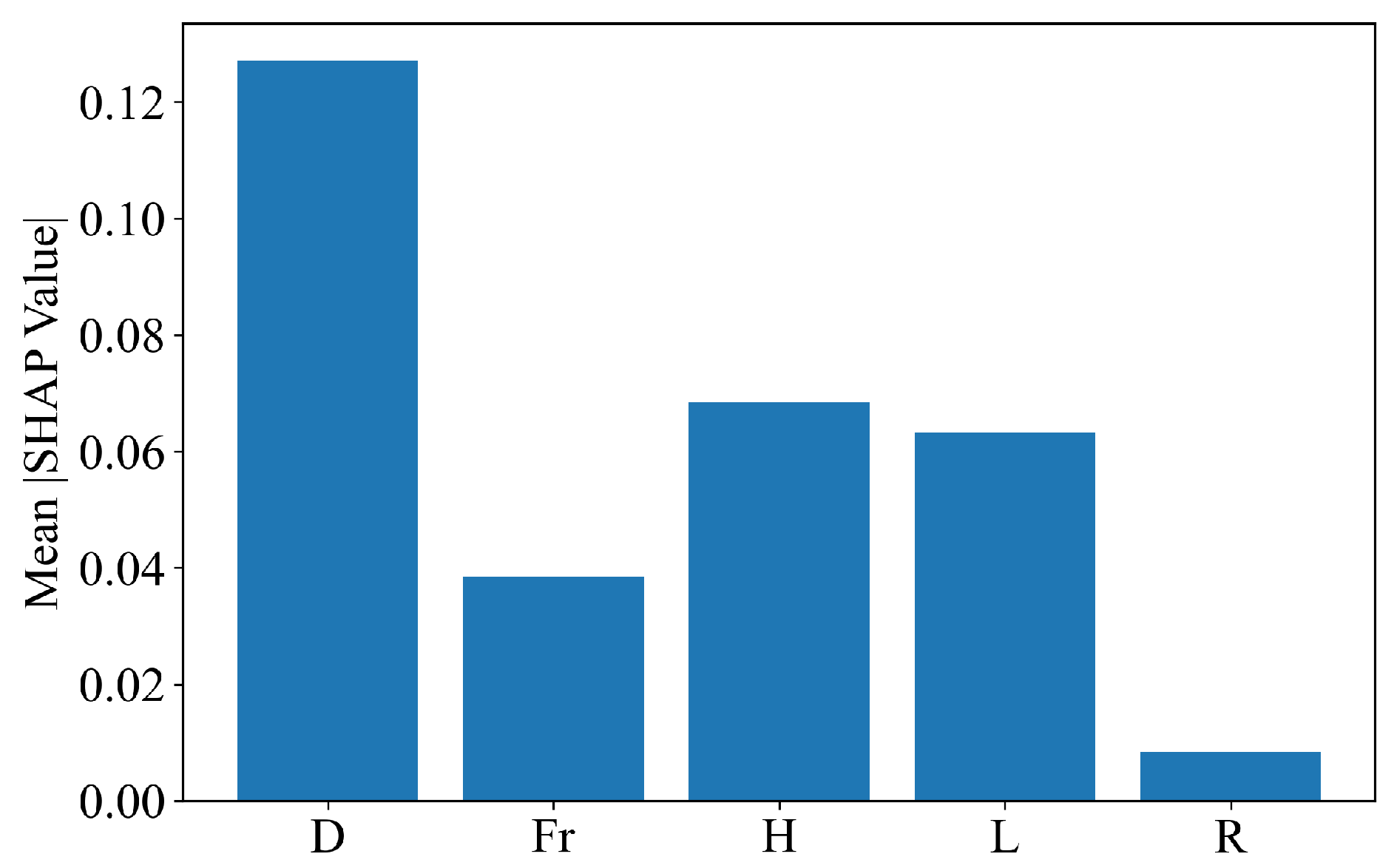
Based on the above evaluation of predictive performance, we selected AE-CatBoost as the tree model to pair with TreeSHAP for subsequent interpretability analysis. AE-CatBoost delivers the highest test R 2 , lowest RMSE and residual variance, and a small train–test gap, indicating strong generalization. This choice supports stable local and global attributions, enables clear quantification of key feature importance and interactions, and provides a more reliable basis for decision-making and model refinement. Figure 19 shows the mean absolute SHAP value of each input variable, helping to quantify each feature’s global contribution to the model output. It can be seen that D is the most dominant input variable with a | SHAP | of 0.125; H and L are the next-most importance influencing factors, while Fr and R provide relatively weak contributions to the run-up distance. The mean | SHAP | quantifies effect size; however, it lacks the information of the affecting direction, that is, whether increasing a feature raises or decreases H m . The affecting direction depends on the local context, and can be shown using a SHAP bee-swarm plot.
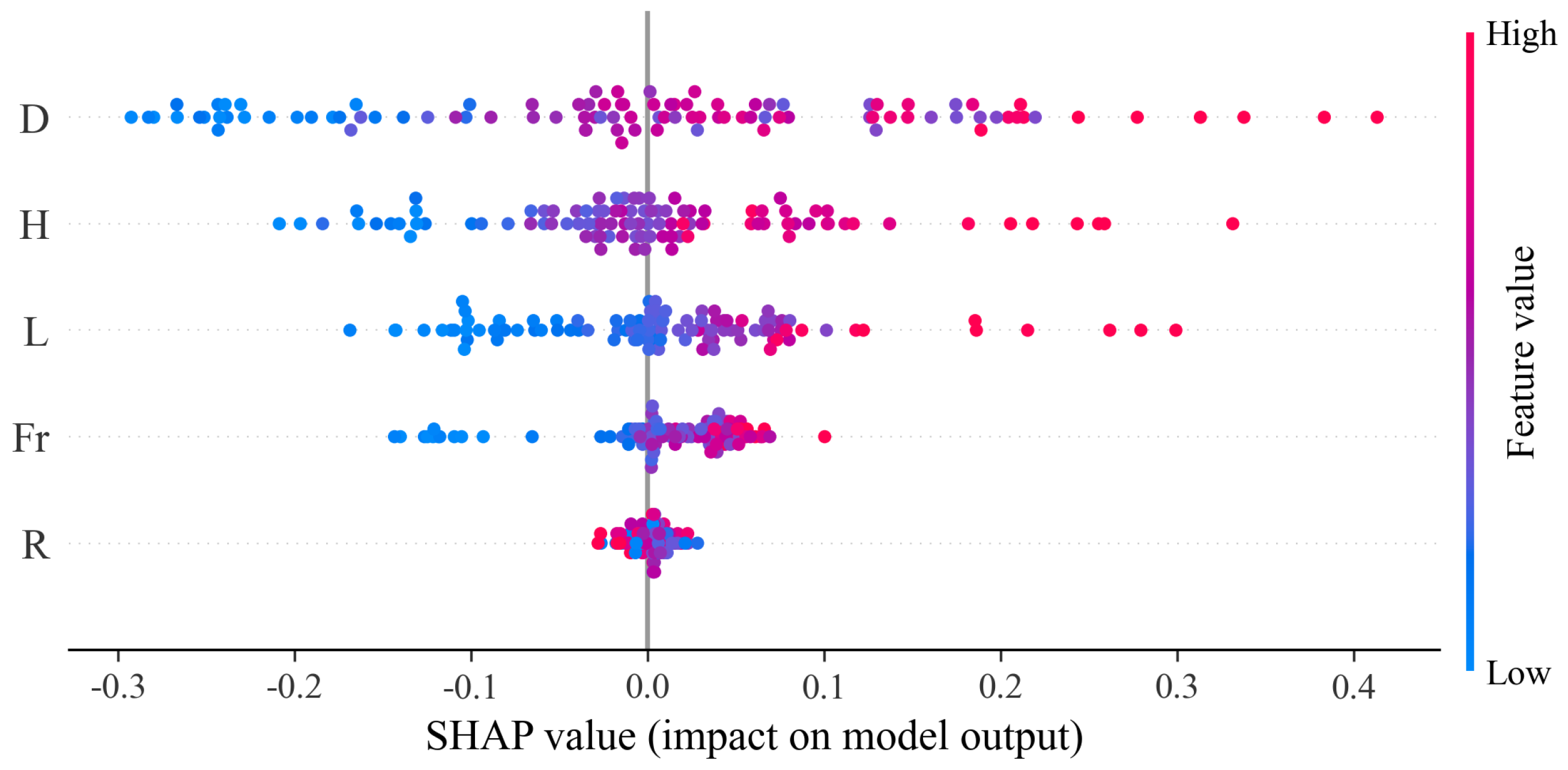
Figure 20 presents the SHAP summary distribution on the basis of the AE-CatBoost model predicting the relative maximum run-up H m . Each dot corresponds to one sample, and the color encodes the feature value from low (blue) to high (red). Red points indicate a local increase in H m , while blue points indicate a decrease. The distribution shows that the relative distance to the dike D is the most influential driver. High D values cluster on the positive side and low D values on the negative side, indicating a near-monotonic positive relationship with H m . Mechanistically, a longer propagation distance allows waves to evolve and shoal over a greater fetch, accumulating momentum before impact and producing higher run-up. The relative wave height H and wavelength L also exhibit clear positive effects. Red points for these two features lie predominantly to the right of zero, showing that taller incident waves and longer relative wavelengths carry more energy and momentum, pushing the uprush farther up the slope and increasing H m . The Froude number Fr shows a similar but weaker pattern; low Fr tends to reduce H m , while high Fr tends to increase it, consistent with greater momentum flux and approach to supercritical conditions enhancing run-up. R contributes only weakly overall, and is centered near zero with a slight negative tendency at higher values. Stronger nonlinearity can trigger earlier breaking and greater energy dissipation, which limits the ultimate uprush and slightly suppresses H m . In summary, the importance ranking is D first, followed by H and L, then Fr , with R exerting the smallest influence. The signs and magnitudes of these effects align with hydrodynamics mechanism: longer propagation distance, larger wave height, longer wavelength, and higher Froude number generally promote larger run-up, whereas stronger nonlinearity tends to damp it through dissipation.
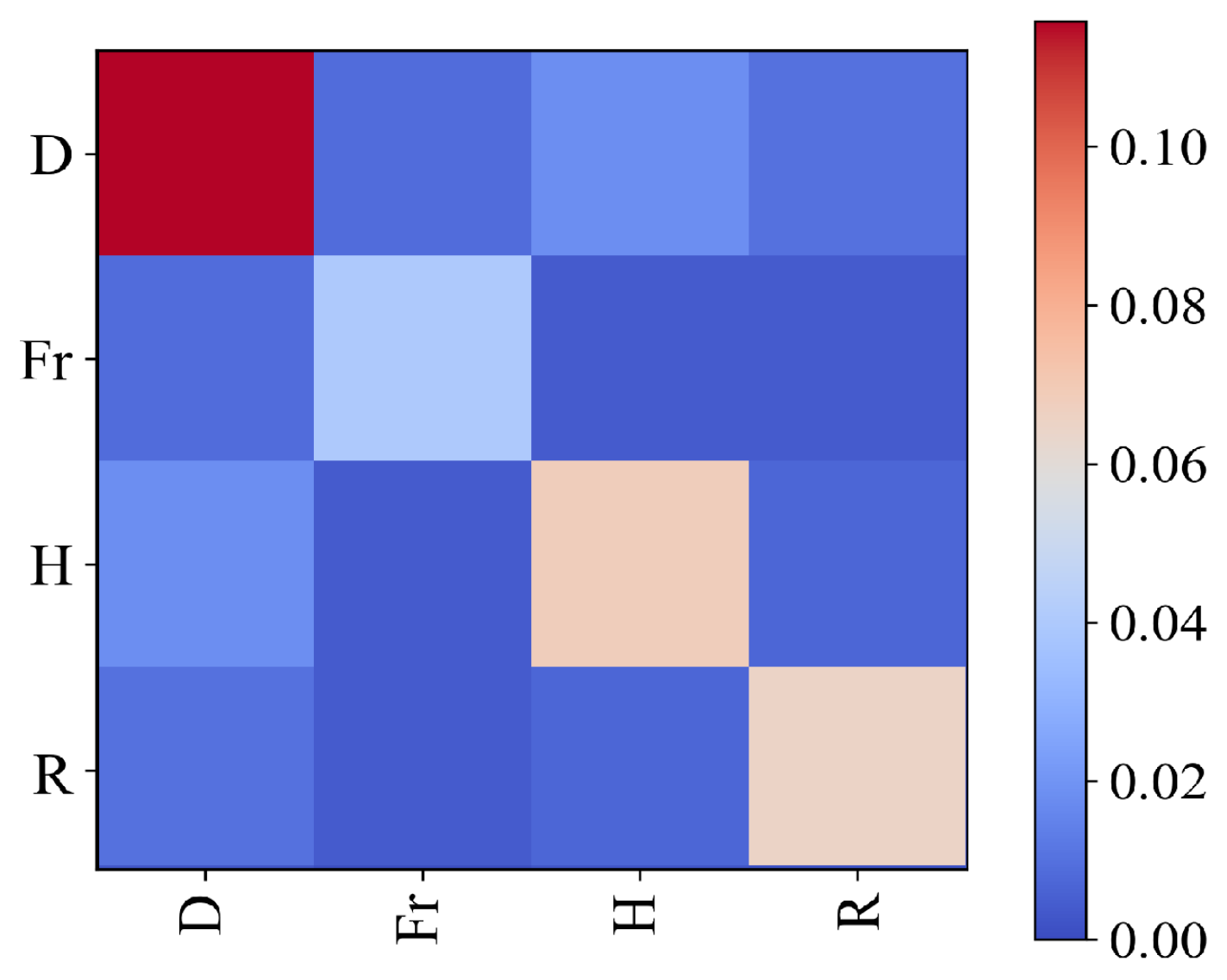
Figure 21 illustrates the heatmap of importance of interaction among each feature. In general, the diagonal terms reflect main effects, where the dominating factor is D, which matches the global importance ranking. The other information obtained from the heatmap is that the most off-diagonal entries are small, indicating a largely additive model. The standout feature interaction is the coupling between H and D, which exceeds all other pairs. Physically, greater wave height combined with a longer relative distance to the dike enhances shoaling and momentum buildup over the propagation path, amplifying uprush more than either factor alone. Interactions involving R remain negligible, consistent with its limited incremental value once H and L are accounted for.

5. Discussion

5.1. Methodological Contribution

Targeting dam break-induced flood propagation and dike overtopping, we establish CatBoost as the baseline and introduce autoencoder-based feature enhancement. AE-CatBoost attains higher test R 2 , lower RMSE and residual variance, and a smaller train–test gap, indicating stronger generalization under the present data and variable setting. The dataset is split into training and test sets by proportional random sampling, without temporal structure; future assessments could add k-fold cross-validation and bootstrap confidence intervals for robustness. Methodologically, this work contributes in two ways: first, we propose a new AE-driven optimization scheme for tree models in which the autoencoder learns compact and physics-aware representations that consistently enhance CatBoost (higher test R 2 , lower RMSE , reduced residual variance); second, we stratify the data by clustering on wave characteristics (relative distance to the dike D, relative wave height H, relative wavelength L, Froude number Fr , and nonlinearity index R) and train a predictive model within each cluster. This yields sharper local fits, captures regime-dependent behavior, and improves interpretability by aligning learned relationships with distinct hydrodynamic regimes.

5.2. Physics-Consistent Interpretability

TreeSHAP analyses provide a global ranking that aligns with the mechanics of dam-break waves impinging on a dike. The relative distance to the dike D is the dominant driver, followed by the relative wave height H and relative wavelength L; the Froude number Fr exerts a weaker but generally positive influence, while the nonlinearity indicator R contributes minimally. SHAP dependence plots reveal nearly monotonic positive effects for D, H, and L, with a strengthening D at 12 to 15, consistent with the idea that once propagation distance is sufficient, shoaling and momentum buildup become more effective and amplify overtopping. The SHAP interaction matrix indicates a largely additive model overall, yet highlights H × D as the strongest coupling: larger incident waves traveling over longer distances accumulate energy and momentum in a way that amplifies run-up beyond simple linear superposition. Note that these attribution patterns are derived from global statistics aggregated over the full dataset, and remain consistent across different wave-regime clusters and train–test splits rather than arising from isolated cases or local effects. This stability across regimes and data partitions reduces the likelihood of coincidental correlations and supports the interpretation that the model has captured robust hydrodynamic mechanisms governing dam-break wave propagation and overtopping.

5.3. Implications for Practice

The dataset was generated using physical model experiments and numerical simulations based on a two-dimensional idealized flume. The present dataset is designed to isolate fundamental hydrodynamic controls such as distance to shoreline, wave height, wavelength, Froude number, and nonlinearity under controlled conditions, thereby enabling robust methodological development and physics-consistent interpretation. While this controlled configuration facilitates systematic parameter variation and physics-consistent learning, it may limit direct extrapolation to real-world terrains characterized by curved channels, irregular cross-sections, vegetation roughness, and built structures. In such environments, additional dissipation, wave scattering, and boundary effects may lead to degradation in predictive performance. Future work will incorporate high-resolution DEMs, realistic boundary conditions, and field observations to quantitatively assess model transferability and robustness.

6. Conclusions

This study investigates dam break-induced flood propagation and dike overtopping. We first benchmarked strong tree learners (XGBoost and ExtraTrees), finding that CatBoost outperforms both. This motivated us to focus our optimization efforts on CatBoost and to develop the AE-optimized variant (AE-CatBoost). Methodologically, we: (i) introduce an alpha evolution (AE) optimization scheme that enhances tree-model predictive accuracy beyond particle swarm optimization (PSO) and grid search (GS); (ii) develop a cluster-wise modeling framework in which regimes are defined by wave characteristics and cases are grouped via hierarchical clustering using Fr , R, and D as clustering criteria; and (iii) establish a physics-consistent interpretability pipeline with SHAP (TreeSHAP) to quantify global importance, local effects, and pairwise interactions.
AE-CatBoost achieves the strongest generalization performance (e.g., test R 2 = 0.9803 , RMSE = 0.0599 ), outperforming the untuned CatBoost baseline, PSO and GS-optimized variants, and alternative tree models including XGBoost and ExtraTrees, with a concurrent reduction in residual variance. By incorporating hierarchical clustering based on Fr , R, and D, the proposed cluster-wise modeling strategy sharpens local fits and better captures regime-dependent behavior. Furthermore, TreeSHAP analyses yield physics-aligned explanations consistently identifying D as the dominant controlling factor, followed by strong positive contributions from H and L, a weaker positive influence of Fr , and a minimal role of R. The interaction between H and D emerges as the strongest coupling, consistent with momentum accumulation during wave propagation over longer distances.
One limitation of this study is that the dataset relies on an idealized flume with simplified topography, which may constrain extrapolation to complex field terrains and boundary conditions. Future work will integrate high-resolution DEMs and realistic boundaries and will adopt robustness-enhancing evaluation such as k-fold cross-validation and uncertainty-aware metrics.

Author Contributions

Conceptualization, H.L. and Z.M.; methodology, Y.F. and Z.M.; validation, X.Z., L.W. and J.Z.; formal analysis, H.L.; writing—original draft preparation, H.L.; writing—review and editing, Z.M.; supervision, L.W.; project administration, H.L.; funding acquisition, H.L. and Z.M. All authors have read and agreed to the published version of the manuscript.

Funding

This research was funded by the Dean’s Research Fund of Zhejiang Institute of Hydraulics & Estuary (Grant No. ZIHE22Q004), the Zhejiang Provincial Natural Science Foundation of China (Grant No.LZJWY24E090005), and the Central Guidance Funds for Science and Technology Local Development Projects (Grant No. 2025ZY01091).

Data Availability Statement

The original contributions presented in this study are included in the article. Further inquiries can be directed to the corresponding author.

Conflicts of Interest

The authors declare no conflicts of interest.

Appendix A. Pseudocode of the Proposed Modeling Procedure

Algorithm A1 illustrates the pseudocode of HC–AE–CatBoost–SHAP modeling. First, the raw dataset is split into training and test sets and wave-related variables are standardized. Agglomerative hierarchical clustering on standardized ( F r , R , D ) is then used to identify wave regimes, which define stratified folds for cross-validation. Alpha evolution (AE) is employed to search CatBoost hyperparameters by minimizing the regime-stratified CV-RMSE, yielding the optimal configuration. A final CatBoost model is trained on the full training set, and TreeSHAP is applied to this model to obtain global feature importance along with local sample-wise explanations for H m .
Algorithm 1 HC–AE-CatBoost–SHAP pseudocode
Require: 
Dataset D = { ( x i , y i ) } i = 1 N
Require: 
Hyperparameter bounds [ lb , ub ]
Require: 
AE population size N pop , maximum function evaluations MaxFEs
Require: 
Candidate cluster numbers k { 2 , , 6 } , number of CV folds K
  1:
Split D into training set D train and test set D test
  2:
On D train , compute μ j , σ j for j { F r , R , D }
  3:
Standardize F r , R , D in both sets using μ j , σ j
                                                                       ▹ Hierarchical clustering on wave features
  4:
Extract standardized ( F r i , R i , D i ) as z i from D train
  5:
for  k = 2 to 6 do
  6:
     Apply agglomerative HC (Ward linkage, Euclidean distance) to obtain partition C k
  7:
     Compute WSS ( C k ) , BSS ( k ) and CH ( k )
  8:
end for
  9:
Set k arg max k CH ( k )
10:
Obtain cluster labels c i for D train under k
11:
Assign labels to D test by nearest-centroid rule
12:
Use { c i } to build wave-regime–stratified K-folds for CV
                                                     ▹ Alpha evolution (AE) hyperparameter optimization
13:
Define decision vector θ = ( d , M , η , λ )
14:
Initialize population X R N pop × d uniformly in [ lb , ub ]
15:
Set function evaluation counter FEs 0
16:
for each individual X i in the population do
17:
       f ( X i ) CV _ RMSE ( X i , D train , { c i } , K )
18:
      FEs FEs + 1
19:
end for
20:
while  FEs < MaxFEs do
21:
     Generate exploratory steps Δ r based on [ lb , ub ]
22:
     Compute progress factor α as a function of FEs
23:
     Construct global reference P via subpopulation aggregation
24:
     for  i = 1 to N pop  do
25:
           Select elite index u and non-elite index v from sorted population
26:
           Set W i X u , L i X v
27:
           Sample perturbation weight vector ϑ i
28:
           Propose trial individual
      E i t + 1 P + α Δ r i + ϑ i ( W i + X i t P L i )
29:
           Project E i t + 1 onto [ lb , ub ] (bound handling)
30:
           Evaluate f ( E i t + 1 ) CV _ RMSE ( E i t + 1 , D train , { c i } , K )
31:
            FEs FEs + 1
32:
           if  f ( E i t + 1 ) f ( X i t )  then
33:
                  X i t + 1 E i t + 1
34:
           else
35:
                  X i t + 1 X i t
36:
           end if
37:
     end for
38:
end while
39:
Select θ as the best individual (minimal f)
                                                                                             ▹ Final training and evaluation
40:
Train CatBoost model F on D train with θ and early stopping
41:
Evaluate F on D test to obtain test RMSE and R 2
                                                                                                            ▹ TreeSHAP analysis
42:
Compute baseline output ϕ 0 = E [ F ( X ) ]
43:
for each sample x i in the dataset do
44:
     Use TreeSHAP to compute ϕ j ( x i ) for j { D , F r , H , L , R }
45:
end for
46:
Compute global importance I j = E x [ | ϕ j ( x ) | ]
47:
Generate global SHAP plots and local explanations from { ϕ j ( x i ) }

References

  1. Saville, T., Jr. Wave run-up on shore structures. J. Waterw. Harb. Div. 1956, 82, 925-1–925-14. [Google Scholar] [CrossRef]
  2. Mather, A.; Stretch, D.; Garland, G. Predicting extreme wave run-up on natural beaches for coastal planning and management. Coast. Eng. J. 2011, 53, 87–109. [Google Scholar] [CrossRef]
  3. Jensen, A.; Pedersen, G.K.; Wood, D.J. An experimental study of wave run-up at a steep beach. J. Fluid Mech. 2003, 486, 161–188. [Google Scholar] [CrossRef]
  4. Stockdon, H.F.; Thompson, D.M.; Plant, N.G.; Long, J.W. Evaluation of wave runup predictions from numerical and parametric models. Coast. Eng. 2014, 92, 1–11. [Google Scholar] [CrossRef]
  5. Peramuna, P.; Neluwala, N.; Wijesundara, K.; DeSilva, S.; Venkatesan, S.; Dissanayake, P. Review on model development techniques for dam break flood wave propagation. Wiley Interdiscip. Rev. Water 2024, 11, e1688. [Google Scholar] [CrossRef]
  6. Kazeminezhad, M.H.; Etemad-Shahidi, A. A new method for the prediction of wave runup on vertical piles. Coast. Eng. 2015, 98, 55–64. [Google Scholar] [CrossRef]
  7. Titov, V.V.; Synolakis, C.E. Numerical modeling of tidal wave runup. J. Waterw. Port Coast. Ocean Eng. 1998, 124, 157–171. [Google Scholar] [CrossRef]
  8. Elliot, R.C.; Hanif Chaudhry, M. A wave propagation model for two-dimensional dam-break flows. J. Hydraul. Res. 1992, 30, 467–483. [Google Scholar] [CrossRef]
  9. Rybkin, A.; Pelinovsky, E.; Didenkulova, I. Nonlinear wave run-up in bays of arbitrary cross-section: Generalization of the Carrier–Greenspan approach. J. Fluid Mech. 2014, 748, 416–432. [Google Scholar] [CrossRef]
  10. Meng, Z.; Zhang, J.; Hu, Y.; Ancey, C. Temporal Prediction of Landslide-Generated Waves Using a Theoretical-Statistical Combined Method. J. Mar. Sci. Eng. 2023, 11, 1151. [Google Scholar] [CrossRef]
  11. Paprotny, D.; Andrzejewski, P.; Terefenko, P.; Furmańczyk, K. Application of empirical wave run-up formulas to the Polish Baltic Sea coast. PLoS ONE 2014, 9, e105437. [Google Scholar] [CrossRef]
  12. Kocaman, S.; Evangelista, S.; Guzel, H.; Dal, K.; Yilmaz, A.; Viccione, G. Experimental and numerical investigation of 3d dam-break wave propagation in an enclosed domain with dry and wet bottom. Appl. Sci. 2021, 11, 5638. [Google Scholar] [CrossRef]
  13. Park, H.; Cox, D.T. Empirical wave run-up formula for wave, storm surge and berm width. Coast. Eng. 2016, 115, 67–78. [Google Scholar] [CrossRef]
  14. Aureli, F.; Dazzi, S.; Maranzoni, A.; Mignosa, P.; Vacondio, R. Experimental and numerical evaluation of the force due to the impact of a dam-break wave on a structure. Adv. Water Resour. 2015, 76, 29–42. [Google Scholar] [CrossRef]
  15. Oppikofer, T.; Hermanns, R.L.; Roberts, N.J.; Böhme, M. SPLASH: Semi-empirical prediction of landslide-generated displacement wave run-up heights. Geol. Soc. Lond. Spec. Publ. 2019, 477, 353–366. [Google Scholar] [CrossRef]
  16. Yang, S.; Yang, W.; Qin, S.; Li, Q.; Yang, B. Numerical study on characteristics of dam-break wave. Ocean Eng. 2018, 159, 358–371. [Google Scholar] [CrossRef]
  17. Girimaji, S.S. Partially-averaged Navier-Stokes model for turbulence: A Reynolds-averaged Navier-Stokes to direct numerical simulation bridging method. J. Appl. Mech. 2006, 73, 413–421. [Google Scholar] [CrossRef]
  18. Haltas, I.; Elçi, S.; Tayfur, G. Numerical simulation of flood wave propagation in two-dimensions in densely populated urban areas due to dam break. Water Resour. Manag. 2016, 30, 5699–5721. [Google Scholar] [CrossRef]
  19. Piomelli, U. Large-eddy simulation: Achievements and challenges. Prog. Aerosp. Sci. 1999, 35, 335–362. [Google Scholar] [CrossRef]
  20. Mendes, D.; Andriolo, U.; Neves, M.G. Advances in wave run-up measurement techniques. In Advances on Testing and Experimentation in Civil Engineering: Geotechnics, Transportation, Hydraulics and Natural Resources; Springer: Cham, Switzerland, 2022; pp. 283–297. [Google Scholar]
  21. Muraki, Y. Field Observations of Wave Pressure, Wave Run-Up, and Oscillation of Breakwater. In Coastal Engineering 1966; American Society of Civil Engineers (ASCE): Reston, VA, USA, 1966; pp. 302–321. [Google Scholar]
  22. Hu, C.; Sueyoshi, M. Numerical simulation and experiment on dam break problem. J. Mar. Sci. Appl. 2010, 9, 109–114. [Google Scholar] [CrossRef]
  23. Casella, E.; Rovere, A.; Pedroncini, A.; Mucerino, L.; Casella, M.; Cusati, L.A.; Vacchi, M.; Ferrari, M.; Firpo, M. Study of wave runup using numerical models and low-altitude aerial photogrammetry: A tool for coastal management. Estuar. Coast. Shelf Sci. 2014, 149, 160–167. [Google Scholar] [CrossRef]
  24. Marangoz, H.O.; Anilan, T. Two-dimensional modeling of flood wave propagation in residential areas after a dam break with application of diffusive and dynamic wave approaches. Nat. Hazards 2022, 110, 429–449. [Google Scholar] [CrossRef]
  25. Yuan, D.; Gu, C.; Wei, B.; Qin, X.; Xu, W. A high-performance displacement prediction model of concrete dams integrating signal processing and multiple machine learning techniques. Appl. Math. Model. 2022, 112, 436–451. [Google Scholar] [CrossRef]
  26. Al-Ghosoun, A.; Gumus, V.; Seaid, M.; Simsek, O. Predicting morphodynamics in dam-break flows using combined machine learning and numerical modelling. Model. Earth Syst. Environ. 2025, 11, 74. [Google Scholar] [CrossRef]
  27. Chen, H.; Huang, S.; Qiu, H.; Xu, Y.P.; Teegavarapu, R.S.; Guo, Y.; Nie, H.; Xie, H.; Xie, J.; Shao, Y.; et al. Assessment of ecological flow in river basins at a global scale: Insights on baseflow dynamics and hydrological health. Ecol. Indic. 2025, 178, 113868. [Google Scholar] [CrossRef]
  28. Khosravi, K.; Sheikh Khozani, Z.; Hatamiafkoueieh, J. Prediction of embankments dam break peak outflow: A comparison between empirical equations and ensemble-based machine learning algorithms. Nat. Hazards 2023, 118, 1989–2018. [Google Scholar] [CrossRef]
  29. Zhang, J.; Zhang, X.; Li, H.; Fan, Y.; Meng, Z.; Liu, D.; Pan, S. Optimization of Water Quantity Allocation in Multi-Source Urban Water Supply Systems Using Graph Theory. Water 2025, 17, 61. [Google Scholar] [CrossRef]
  30. Chen, H.; Xu, B.; Qiu, H.; Huang, S.; Teegavarapu, R.S.; Xu, Y.P.; Guo, Y.; Nie, H.; Xie, H. Adaptive assessment of reservoir scheduling to hydrometeorological comprehensive dry and wet condition evolution in a multi-reservoir region of southeastern China. J. Hydrol. 2025, 648, 132392. [Google Scholar] [CrossRef]
  31. Meng, Z.; Hu, Y.; Jiang, S.; Zheng, S.; Zhang, J.; Yuan, Z.; Yao, S. Slope Deformation Prediction Combining Particle Swarm Optimization-Based Fractional-Order Grey Model and K-Means Clustering. Fractal Fract. 2025, 9, 210. [Google Scholar] [CrossRef]
  32. Power, H.E.; Gharabaghi, B.; Bonakdari, H.; Robertson, B.; Atkinson, A.L.; Baldock, T.E. Prediction of wave runup on beaches using Gene-Expression Programming and empirical relationships. Coast. Eng. 2019, 144, 47–61. [Google Scholar] [CrossRef]
  33. Rehman, K.; Khan, H.; Cho, Y.S.; Hong, S.H. Incident wave run-up prediction using the response surface methodology and neural networks. Stoch. Environ. Res. Risk Assess. 2022, 36, 17–32. [Google Scholar] [CrossRef]
  34. Li, Y.; Peng, T.; Xiao, L.; Wei, H.; Li, X. Wave runup prediction for a semi-submersible based on temporal convolutional neural network. J. Ocean Eng. Sci. 2024, 9, 528–540. [Google Scholar]
  35. Naeini, S.S.; Snaiki, R. A physics-informed machine learning model for time-dependent wave runup prediction. Ocean Eng. 2024, 295, 116986. [Google Scholar] [CrossRef]
  36. Li, Y.; Xiao, L.; Wei, H.; Li, D.; Li, X. A comparative study of LSTM and temporal convolutional network models for semisubmersible platform wave runup prediction. J. Offshore Mech. Arct. Eng. 2025, 147, 011202. [Google Scholar] [CrossRef]
  37. Li, J.; Meng, Z.; Zhang, J.; Chen, Y.; Yao, J.; Li, X.; Qin, P.; Liu, X.; Cheng, C. Prediction of Seawater Intrusion Run-Up Distance Based on K-Means Clustering and ANN Model. J. Mar. Sci. Eng. 2025, 13, 377. [Google Scholar] [CrossRef]
  38. Wang, H.; Liang, Q.; Hancock, J.T.; Khoshgoftaar, T.M. Feature selection strategies: A comparative analysis of SHAP-value and importance-based methods. J. Big Data 2024, 11, 44. [Google Scholar] [CrossRef]
  39. Van den Broeck, G.; Lykov, A.; Schleich, M.; Suciu, D. On the tractability of SHAP explanations. J. Artif. Intell. Res. 2022, 74, 851–886. [Google Scholar] [CrossRef]
  40. Murtagh, F.; Contreras, P. Algorithms for hierarchical clustering: An overview. Wiley Interdiscip. Rev. Data Min. Knowl. Discov. 2012, 2, 86–97. [Google Scholar] [CrossRef]
  41. Contreras, P.; Murtagh, F. Hierarchical clustering. In Handbook of Cluster Analysis; CRC Press: Boca Raton, FL, USA, 2015; pp. 103–123. [Google Scholar]
  42. Ran, X.; Xi, Y.; Lu, Y.; Wang, X.; Lu, Z. Comprehensive survey on hierarchical clustering algorithms and the recent developments. Artif. Intell. Rev. 2023, 56, 8219–8264. [Google Scholar] [CrossRef]
  43. Prokhorenkova, L.; Gusev, G.; Vorobev, A.; Dorogush, A.V.; Gulin, A. CatBoost: Unbiased boosting with categorical features. arXiv 2018, arXiv:1706.09516. [Google Scholar]
  44. Gao, H.; Zhang, Q. Alpha evolution: An efficient evolutionary algorithm with evolution path adaptation and matrix generation. Eng. Appl. Artif. Intell. 2024, 137, 109202. [Google Scholar] [CrossRef]
  45. Inan, M.S.K.; Rahman, I. Explainable AI integrated feature selection for landslide susceptibility mapping using TreeSHAP. SN Comput. Sci. 2023, 4, 482. [Google Scholar] [CrossRef]
  46. Kopanja, M.; Hačko, S.; Brdar, S.; Savić, M. Cost-sensitive tree SHAP for explaining cost-sensitive tree-based models. Comput. Intell. 2024, 40, e12651. [Google Scholar] [CrossRef]
  47. Li, Z. Extracting spatial effects from machine learning model using local interpretation method: An example of SHAP and XGBoost. Comput. Environ. Urban Syst. 2022, 96, 101845. [Google Scholar] [CrossRef]
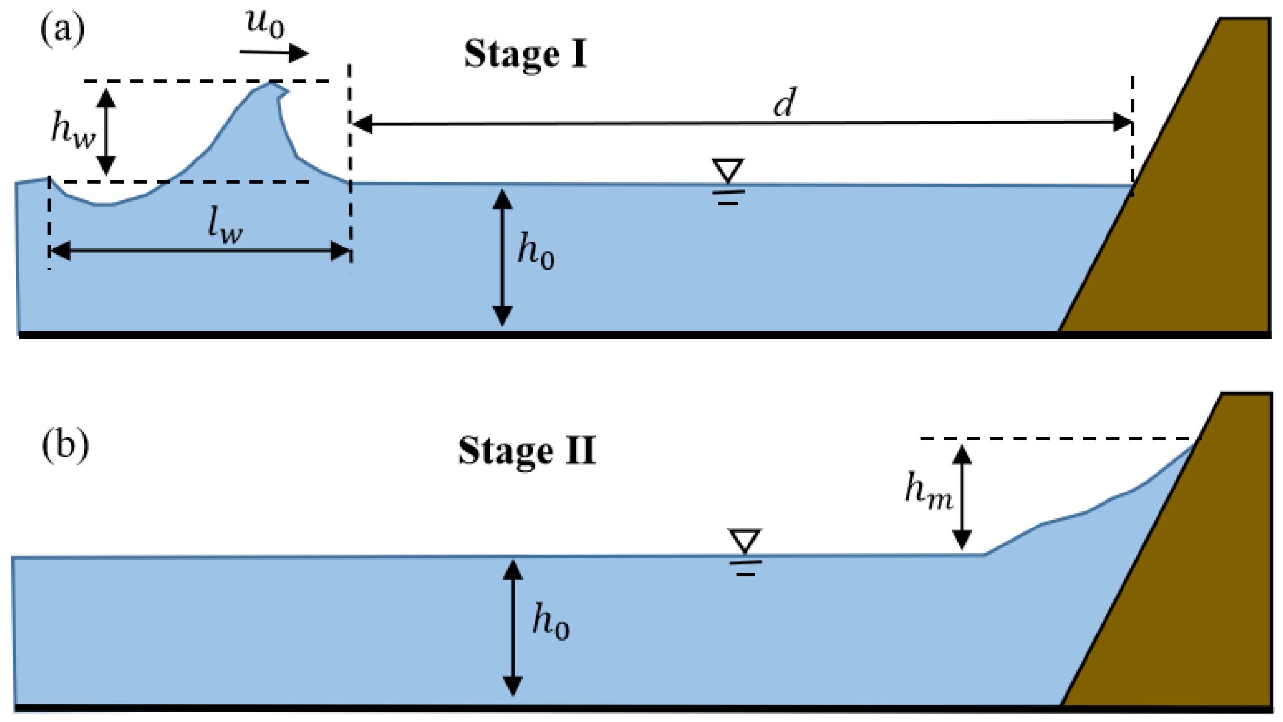
Figure 1. Physical model of impulse-wave propagation: (a) initial stage and (b) impacting stage.
Water 18 00042 g001
Figure 2. Sketch of the two-dimensional experimental flume with a dike.
Water 18 00042 g002
Figure 3. Representative snapshots of the dam break-induced impulse wave impacting and overtopping the dike.
Water 18 00042 g003
Figure 4. Velocity magnitude of a dam break-induced impulse wave during propagation and overtopping at t = 0.00 s, 1.00 s, 1.09 s, and 2.20 s, obtained from SPH numerical simulations.
Water 18 00042 g004
Figure 5. The distribution of the five input variables: (a) D, (b) Fr , (c) H, (d) L, (e) R.
Water 18 00042 g005
Figure 6. Overall flow of the HC–AE–CatBoost–SHAP modeling process.
Water 18 00042 g006
Figure 7. The principle of the hierarchical clustering (HC) method.
Water 18 00042 g007
Figure 8. Principle of the CatBoost algorithm.
Water 18 00042 g008
Figure 9. Alpha evolution (AE) hyperparameter optimization for CatBoost.
Water 18 00042 g009
Figure 10. Principle of the interpretation model based on a tree-based prediction model and SHAP analysis.
Water 18 00042 g010
Figure 11. Pearson correlation heatmap of the five input variables ( D , Fr , H , L , R ).
Water 18 00042 g011
Figure 12. Selection of optimal cluster number based on CH index.
Water 18 00042 g012
Figure 13. The evolution of ward distance of all samples distinguishing the two clusters.
Water 18 00042 g013
Figure 14. The pairwise scatter plots and marginal histograms in ( Fr , R , D ) space distinguishing the two clusters.
Water 18 00042 g014
Figure 15. The 3D scatter in ( Fr , R , D ) space distinguishing the two clusters.
Water 18 00042 g015
Figure 16. Comparison of the predicted and recorded data for both training data and testing data: (a) CatBoost, (b) AE-CatBoost, (c) XGBoost, (d) ExtraTrees, (e) PSO-CatBoost, (f) GS-CatBoost.
Water 18 00042 g016
Figure 17. Radar plots of (a) R 2 and (b) RMSE for the six prediction models.
Water 18 00042 g017
Figure 18. Histogram of residual of the six prediction models: (a) training data and (b) testing data.
Water 18 00042 g018
Figure 19. The absolute mean SHAP values of the five explanatory variables.
Water 18 00042 g019
Figure 20. SHAP summary distribution based on the AE-CatBoost model.
Water 18 00042 g020
Figure 21. Mean absolute SHAP value, indicating the interaction among each feature.
Water 18 00042 g021
Disclaimer/Publisher’s Note: The statements, opinions and data contained in all publications are solely those of the individual author(s) and contributor(s) and not of MDPI and/or the editor(s). MDPI and/or the editor(s) disclaim responsibility for any injury to people or property resulting from any ideas, methods, instructions or products referred to in the content.