A Study on Seepage Pressure Forecasting for Concrete Dams Based on Multi-Scale Preprocessing and Dual-Model Integration

Abstract

Seepage pressure time series of concrete dams are governed by reservoir water level, rainfall, temperature and long-term aging effects, featured by strong nonstationarity and complex multi-scale fluctuations. Existing decomposition–ensemble methods ignore nonlinear coupling among scale components, suffering low prediction accuracy and poor physical interpretability. Current model fusion schemes fail to adapt to differentiated evolution mechanisms of frequency-varying seepage components and cannot fully mine implicit cross-scale nonlinear correlations. To overcome these drawbacks, this study proposes a concrete dam seepage pressure prediction approach integrating ensemble empirical mode decomposition, multi-scale preprocessing, and optimized dual-model selection combining ridge regression and Transformer–BiLSTM. Ensemble empirical mode decomposition adaptively denoises and decouples raw seepage series into high-, medium- and low-frequency IMFs according to oscillation cycles. A normalized Comprehensive Optimization Index is constructed to parallelly train ridge regression and Transformer–BiLSTM for each component and select the optimal submodel dynamically. A fully connected nonlinear fusion layer reconstructs multi-scale predictions to retain inherent component coupling features, replacing traditional simple linear superposition. Engineering cases verify that the proposed model efficiently captures periodic laws of key influencing factors, significantly boosting prediction accuracy and generalization capacity, thus possessing prominent theoretical and practical engineering application values.

1. Introduction

Concrete dams are critical national strategic infrastructure pivotal to water resource allocation, flood regulation, and hydropower supply [1]. Seepage pressure is a core physical quantity characterizing the spatiotemporal evolution of seepage fields in concrete dams, and its abnormal time-series fluctuations and trend deviations commonly precede structural defects such as contact erosion, and seepage instability [2,3]. Accordingly, developing high-accuracy, strongly generalizable seepage pressure prediction methods has become a core research priority in safety monitoring and risk identification for in-service concrete dams [4,5].

Seepage pressure prediction models for concrete dams take upstream and downstream water levels, rainfall, and aging effects as independent variables to map seepage pressure, with prevailing frameworks covering statistical, machinelearning, and deep-learning models [6,7]. Statistical models select influencing factors based on engineering experience or seepage field analysis and calibrate parameters via data analysis; integrated with physical mechanisms throughout modeling, they are widely adopted in engineering practice [8]. However, multiple driving factors and inherent uncertainties in seepage behavior [9] render seepage pressure data highly nonlinear, nonstationary and multi-scale coupled, imposing strict requirements on models for multi-scale feature decoupling, nonlinear correlation mining and long-term temporal dependency capture.

With advances in computing technology, machine learning methods have been increasingly applied to seepage pressure prediction for concrete dams [10,11]. However, existing studies indicate that traditional machine learning models are limited by excessive manual intervention and a tendency to lose physical features of raw data [12,13]. Concrete dam monitoring data features intense fluctuations, high noise, and deep coupling between long-period trends and short-period oscillations [14]. Single models consistently fail to balance long-term trend fitting and local fluctuation capture, while combining outputs from multiple models mitigates overfitting and underfitting risks to improve prediction performance [15,16]. To address these shortcomings of traditional and single models, scholars worldwide have conducted extensive studies on structural optimization and multi-method integration. Xie et al. [17] addressed two key bottlenecks of deep learning models in this field: inadequate characterization of nonlinear temporal relationships and poor interpretability. They developed an AE-BiGRU prediction model optimized by the Alpha evolutionary algorithm and quantified the contribution of each driving factor via SHAP interpretability analysis. Chen et al. [18] proposed a prediction method based on CNN–Attention–LSTM to resolve the issue that existing models cannot fully capture nonlinear relations among multiple influencing factors. Zhu et al. [19] tackled the problem that raw dam foundation seepage monitoring data is susceptible to environmental noise, while conventional denoising methods often lose detailed features. They put forward a denoising preprocessing scheme integrating variational mode decomposition and wavelet packets, constructed an improved temporal convolutional network model, and optimized its structure by incorporating the hysteresis characteristics of seepage pressure. In recent years, decomposition–ensemble approaches have attracted extensive research attention owing to their capacity to effectively address the inherent nonstationarity and multi-scale coupling characteristics embedded in dam monitoring datasets [20]. Rezaie-Balf et al. [21] adopted complete ensemble empirical mode decomposition with adaptive noise (CEEMDAN) to separate multi-frequency components from streamflow time series, where three machine learning algorithms including MARS, ANN and M5-MT were individually matched for component-wise prediction before sequence reconstruction. Fatehi-Nobarian et al. [22] implemented discrete wavelet transform to realize the multi-scale decomposition of seepage pressure time series and fed the decomposed high- and low-frequency sub-sequences into neural networks for parallel modeling and ensemble forecasting. Collectively, these studies verify that multi-scale preprocessing is indispensable for capturing the intricate evolutionary patterns of dam seepage monitoring data. Nevertheless, the majority of existing decomposition–ensemble frameworks still adopt a unified model architecture for all decomposed components and merely utilize linear superposition to accomplish final signal reconstruction. In terms of modeling after multi-scale decoupling, Wei et al. [23] took the chaotic and periodic characteristics of residual sequences from hybrid models into consideration and adopted the Extreme Learning Machine (ELM) and Seasonal Autoregressive Integrated Moving Average (SARIMA) to conduct separate modeling and prediction for high-frequency and low-frequency signals, respectively. Wang et al. [24] proposed a structured decoupled prediction model named DTSformer. By virtue of a multi-scale moving average decomposition strategy, the original time series was decomposed into trend components and seasonal periodic components, with dedicated modeling architectures custom-designed for each component category. From the perspective of data reconstruction, Kong et al. [25] combined composite entropy with the K-means algorithm to realize the division of high-frequency and low-frequency modes, and subsequently adopted linear superposition to implement progressive nonlinear time series reconstruction across dual layers of modes.

Previous studies indicate that seepage pressure prediction models for concrete dams are far less developed than those for earth rock dams, and research on the underlying physical driving mechanisms remains notably insufficient, resulting in prominent black-box limitations. Affected by multiple loads, concrete dam seepage pressure typically forms nonstationary time series. Directly feeding raw data into machine learning models leads to slow convergence and unsatisfactory accuracy during iteration. Mode decomposition methods can address this issue by splitting nonstationary sequences, training each component separately via machine learning algorithms, and fusing the outputs. However, existing studies generally adopt a unified model to fit all monitoring data while ignoring inherent differences in seepage pressure evolution patterns. Model selection strongly influences prediction results, making it difficult to simultaneously deliver long-term trend fitting and short-term fluctuation capture. Even repeated parameter tuning fails to balance these two objectives. Most ensemble models also generate final predictions through linear superposition, which cannot capture nonlinear interactions across multiscale components and often loses correlation information between components.

To overcome these limitations, this paper proposes a concrete dam seepage pressure prediction method combining EEMD multiscale preprocessing with dual model optimal matching. The EEMD method decomposes raw seepage pressure time series via adaptive noise-assisted processing—yielding low, medium and high frequency fluctuation components with clear physical interpretations. A differentiated dual model framework is constructed, and a normalized Comprehensive Optimization Index (hereinafter abbreviated as COI) is established to enable dynamic model adaptation. Specifically, ridge regression is applied to low-frequency trend components, while the Transformer–BiLSTM network handles medium- and high-frequency nonlinear fluctuation components, ensuring predictions capture both long-term patterns and short-term fluctuations. Finally, a nonlinear fusion layer completes the global sequence reconstruction of multicomponent prediction results. Comparative and ablation experiments based on long-term monitoring data from a large concrete hyperbolic arch dam validate the accuracy of the proposed model.

The main contributions of this study are as follows: (1) an EEMD multi-scale decomposition scheme adapted to seepage pressure time series is established. This scheme achieves the physical decoupling of seepage features at different time scales and employs different models to fit components with distinct seepage characteristics; (2) a COI-driven parallel optimal selection strategy for the two candidate models is proposed, matching appropriate modeling methods for components with different frequency properties.

2. Methodology

2.1. Seepage Pressure Statistical Model

The seepage pressure statistical model is the most mature empirical approach for concrete dam safety monitoring, integrating fundamental seepage mechanics theories with long-term observed engineering patterns. It decomposes measured seepage pressure time series from dam bodies and foundations into physically meaningful driving components and establishes quantitative mappings between influencing factors and seepage pressure responses via multiple regression analysis [26,27].

The evolution of foundation uplift pressure and dam body seepage pressure in concrete dams is governed by four categories of factors: upstream–downstream water head difference, rainfall infiltration, periodic temperature fluctuation, and long-term temporal dependence [28]. Limited by the physical properties of fractured foundation rock masses and permeable dam concrete media, changes in reservoir water level and rainfall cannot transmit instantaneously to monitoring sections [29]. Seepage pressure responses thus show an obvious lag effect relative to external loads, so multi-period average factors are introduced to characterize this delayed transmission process. Accordingly, the statistical model can be decomposed into four components: water-pressure-, rainfall-, temperature- and time-dependent components. Its general expression is as follows:

$$\begin{array}{cc}\hfill H& =H_h+H_p+H_t+H_{\theta }\hfill \\ & =z+{\displaystyle {\displaystyle \sum _{i=1}^7}{a}_i}\left(h_i-h_{0i}\right)+{\displaystyle {\displaystyle \sum _{i=1}^4}{c}_i}\left(p_i-p_{0i}\right)\hfill \\ & +{\displaystyle \sum _{i=1}^2\left[b_{1i}\left(\sin \frac{2\mathsf{\pi }it}{365}-\sin \frac{2\mathsf{\pi }i{t}_0}{365}\right)+b_{2i}\left(\cos \frac{2\mathsf{\pi }it}{365}-\cos \frac{2\mathsf{\pi }i{t}_0}{365}\right)\right]}+k_t\left(t-t_0\right)\hfill \\ & +d_1\left(\theta -{\theta }_0\right)+d_2\left(\ln \theta -\ln {\theta }_0\right)\hfill \end{array}$$

(1)

where H is the measured seepage pressure on the monitoring day; z is the constant term of the model; and $H_h,H_p,H_t,H_{\theta }$ are respectively the water-pressure component, rainfall component, temperature component and time-dependent component. t is the cumulative days counted from the starting date of monitoring and $t_0$ is the cumulative days on the initial monitoring date.

(1)

Water-Pressure Component

The water head difference between upstream and downstream directly governs the hydraulic gradient in the dam body and foundation. To account for the temporal lag of seepage transmission, seven water head difference factors are defined. Where $h_i$ is the average upstream–downstream water head difference for seven time windows—the monitoring day, 1 day before monitoring, 2–4 days prior, 5–15 days prior, 16–30 days prior, 31–60 days prior, and 61–100 days prior—and $h_{0i}$ is the average water head difference of the identical intervals on the initial monitoring day. $a_i$ is the regression coefficients associated with each water-pressure factor. Integrating multi-scale lagged water head factors effectively quantifies the cumulative lag response of seepage pressure to water head variations and reproduces unsteady seepage propagation.

(2)

Rainfall Component

Rainfall disturbs the seepage field through two primary pathways: rock-fracture infiltration and groundwater recharge around the reservoir area, with its influence also showing a notable time lag. Four grades of rainfall factors are set to quantify rainfall intensity and lagged effects. Where $p_i$ is the average rainfall over four time windows—the monitoring day, 1 day before monitoring, 2–4 days prior, and 5–8 days prior—and $p_{0i}$ is the average rainfall of the corresponding time windows on the initial monitoring day. $c_i$ is the regression coefficient matching each rainfall factor. Rainfall-insensitive riverbed points may drop or simplify the rainfall component via correlation analysis.

(3)

Temperature Component

Temperature variation is a key driver of periodic seepage pressure fluctuations. The thermal expansion and contraction of dam concrete and foundation rock masses alter fracture apertures and pore structures, leading to periodic changes in permeability coefficient. Structural deformation caused by thermal stress indirectly changes the connectivity of seepage flow channels. The temperature field of concrete dams features dominant annual and semiannual cyclic variations, so a dual harmonic function is adopted for the temperature component Where i = 1 is the annual periodic fluctuations, and i = 2 is the semi-annual periodic fluctuations. $b_{1i}$ and $b_{2i}$ are the regression coefficients of the temperature component for periodic oscillation terms. This form accurately fits temperature periodic variations in seepage pressure. Long-term climate warming drift term $k_t\left(t-t_0\right)$ quantifies the cumulative background temperature rise induced by global warming over decades; coefficient $k_t$ is solved synchronously with other regression parameters. Daily temperature fluctuations, though potentially intensified by climate warming, are rapidly attenuated in the dam body and foundation due to thermal inertia, so their direct influence on deep-seated seepage pressure is therefore limited compared to seasonal effects.

(4)

Time-Dependent Component

The time-dependent component describes the irreversible evolution of the seepage field during long-term service of concrete dams, originating from multiple physical mechanisms including creep deformation of foundation rock masses, sediment silting and chemical dissolution inside seepage channels, and damage evolution of dam concrete. The processes typically show decaying features, with fast change rates at the early stage and gradual stabilization at the later stage. A combined form of linear and logarithmic terms is thus adopted for fitting, where $\theta$ is the normalized time-dependent factor, with $\theta =0.01t$, and ${\theta }_0$ is the corresponding time-dependent factor on the initial monitoring day. $d_1$ and $d_2$ are the regression coefficients of the time-dependent component. The linear term characterizes the steady long-term evolutionary trend. The logarithmic term captures decaying consolidation and time-dependent behaviors relating to creep. It should be recognized that the proposed statistical model will be adjusted according to the actual situation on-site. Lithology-specific creep characteristics are implicitly reflected through the site-specific time-dependent coefficients rather than through explicit petrophysical parameters. For highly heterogeneous foundations, incorporating lithology indices (e.g., RMR, weathering grade) as additional regressors could enhance physical interpretability. Furthermore, concrete damage evolution often exhibits spatial heterogeneity between the upstream and downstream faces, where thermal gradients, freeze–thaw cycles, and carbonation rates differ markedly, which are amplified at altitudes exceeding 1800 m. Spatially differentiated or elevation-corrected modeling strategies are therefore recommended for such environments to account for asymmetric deterioration patterns.

The seepage pressure statistical model is essentially a multiple linear regression model. The least squares method is generally used to solve the regression coefficients of each component. For concrete dams under normal steady operating conditions, it has been widely applied in seepage pressure fitting and trend analysis. Nevertheless, the model is built upon the linear superposition assumption. It cannot accurately capture the strong nonlinearity and nonstationarity of seepage pressure time series under multi-field coupling effects [30,31]. In addition, its fixed factor structure fails to adaptively mine deep temporal dependencies hidden in monitoring data. So nonlinear approaches including signal decomposition and deep learning need to be introduced to improve the original model.

It is worth noting that the current statistical predictive framework characterizes foundation geological effects merely via implicit correction terms embedded within the time-dependent regression coefficients. To overcome this simplified treatment, future model optimization will integrate an explicit multifactor weighting scheme within the parametric framework to quantitatively characterize various critical geological attributes. The geological indicators to be incorporated include lithology categories, in situ geomechanical parameters, spatial fracture distribution, schistosity development degree, chemically banded structures, hydrogeochemical dissolution and reprecipitation processes, as well as rock mechanical properties and weathering susceptibility. Benefiting from the refined parametric coupling described above, the model can deliver more robust validation results with complete physical mechanisms and enhanced adaptability to complex and extreme engineering scenarios.

2.2. Ensemble Empirical Mode Decomposition (EEMD)

In the monitoring of concrete dams, seepage pressure data are controlled by coupled multiple factors and exhibit nonlinear and nonstationary characteristics. Ensemble empirical mode decomposition (EEMD) is a noise-assisted signal analysis method proposed by Wu and Huang based on empirical mode decomposition (EMD) [32]. EEMD completes signal decomposition purely according to the intrinsic time-scale features of the original signal. It does not require the manual setting of priori parameters. This method has natural adaptability for processing seepage pressure monitoring sequences of concrete dams.

EMD forms the theoretical basis of EEMD via layered screening of complex nonstationary signals. It can decompose a nonstationary signal $x\left(t\right)$ into several intrinsic mode function (IMF) components $c_i\left(t\right)$ and one residual trend term $r\left(t\right)$:

$$x\left(t\right)={\displaystyle \sum _{i=1}^n{c}_i\left(t\right)}+r\left(t\right)$$

(2)

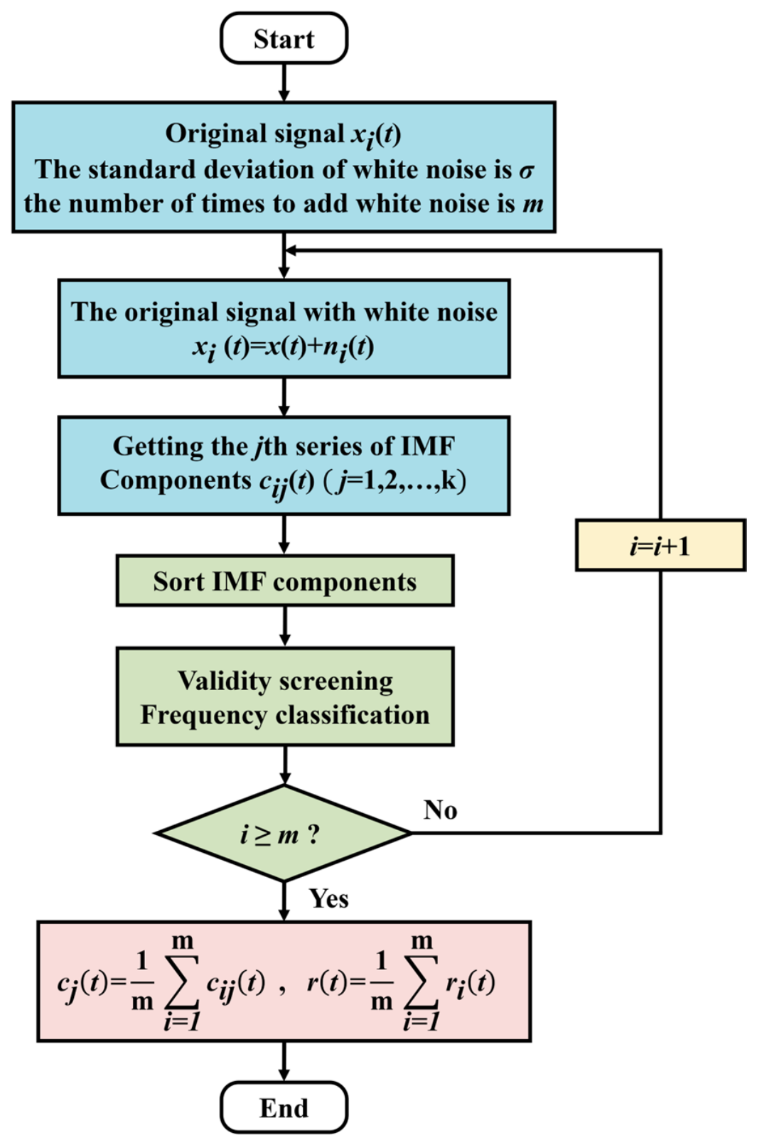
This decomposition process is fully driven by the features of the signal itself. It requires no predefined basis functions and can effectively reflect physical fluctuations at distinct time scales. However, if the raw signal contains intermittent disturbances, random noise or abrupt variations, modal aliasing will emerge in decomposition results. To address this defect, EEMD repeatedly injects white noise with a mean of zero into the original signal. Then, extreme points are evenly distributed across the whole signal. Modal aliasing is thereby suppressed, and the adaptive multi-scale decomposition of nonlinear, nonstationary time series signals is realized. The implementation workflow of the EEMD method adopted is illustrated in Figure 1, detailed as follows:

(1) Parameter initialization and noisy signal generation: set the standard deviation $\sigma$ of white noise and the noise superposition times m according to the temporal resolution and fluctuation features of seepage pressure monitoring data from concrete dams. Add the group i white noise $n_i\left(t\right)$ to the original signal $x\left(t\right)$ to obtain a new time series $x_i\left(t\right)$, thus completing the reconstruction of noisy signals:

$$x_i\left(t\right)=x\left(t\right)+n_i\left(t\right)$$

(3)

(2) Sequential EMD: Perform EMD on each noisy time series $x_i\left(t\right)$ to obtain the group j of IMF component $c_{ij}\left(t\right)$ and residual $r_i\left(t\right)$. Accumulate all m groups of decomposition results.

(3) Ensemble Averaging for Noise Elimination: Compute ensemble averages over the m groups of IMF components and residuals to acquire the final averaged IMF $c_j\left(t\right)$ and averaged residual $r\left(t\right)$:

$$c_j\left(t\right)={\displaystyle \frac{1}{m}}{\displaystyle \sum _{i=1}^m{c}_{ij}\left(t\right)}$$

(4)

$$r\left(t\right)={\displaystyle \frac{1}{m}}{\displaystyle \sum _{i=1}^m{r}_i\left(t\right)}$$

(5)

(4) Component Screening and Frequency Classification: process decomposed IMF components under dual criteria: quantitative validity screening and engineering physical period threshold:

a. Validity Screening: eliminate invalid components without physical interpretation via four quantitative indicators. The screening formulas are expressed as

$$\left\{\begin{array}{l}{L}_{IM{F}_i}\ge L_{min}\\ E_{IM{F}_i}={\displaystyle \sum _{k=1}^{N}IM{F}_{ik}^2}>{10}^{-10}\\ Var\left(IM{F}_i\right)>{10}^{-12}\\ \left|Corr\left(IM{F}_i,y_{raw}\right)\right|>0.01\end{array}\right.$$

(6)

where $L_{IM{F}_i}$ is the effective length of the i-th IMF component; and $L_{min}$ is the minimum effective length, determined by prediction window and sample size requirements; $E_{IM{F}_i}$ is the energy of the i-th IMF component; N is the total number of data points of the IMF component; $Var\left(IM{F}_i\right)$ is the variance of the i-th IMF component; and $Corr\left(IM{F}_i,y_{raw}\right)$ is the Pearson correlation coefficient between the i-th IMF component and the original seepage pressure sequence $y_{raw}$ of the dam body.

b. Frequency Classification: severe valid IMF components are screened. Based on the engineering periodic characteristics of seepage pressure evolution in concrete dams, these components are divided into three categories. High frequency (period < 7 days): Short-term random measurement noise and instantaneous rainfall disturbance, dominated by small random fluctuations without obvious continuous regularities. Medium frequency (period 7–30 days): Seepage pressure responses driven by environmental loads including reservoir water level fluctuation and periodic temperature variation, featuring strong nonlinear temporal dependence and lagged fluctuations. Low frequency (period > 30 days): Trend terms reflecting long-term evolution of seepage channels, impervious curtain and rock mass permeability in dam foundations, dominated by gentle linear trends.

After the above processing, the IMFs decomposed by EEMD are arranged from high to low frequency and from short to long period. Each component corresponds to a distinct physical driving mechanism of seepage pressure variation. This method retains all time scale fluctuation features of seepage fields, separates complex seepage pressure changes caused by multiple factors, and offers high-quality data for multi-scale modeling and full seepage pressure sequence reconstruction.

2.3. Ridge Regression

As a classical parametric modeling method, linear regression fits the linear correlation between input features and output responses by minimizing the sum of squared residuals. Its basic form is written as

$$y=\mathit{X}\mathit{\beta }+\epsilon$$

(7)

The corresponding loss function is

$$L(\mathit{\beta })={\displaystyle \sum _{i=1}^n{(y_i-{\mathit{X}}_i\mathit{\beta })}^2}$$

(8)

where y is the measured seepage pressure response of the dam; $\mathit{X}\in {\mathbb{R}}^{n\times p}$ is the p-dimensional feature matrix of seepage driving factors including reservoir water level, temperature and time-dependent terms; n is the total sample size; $\mathit{\beta }\in {\mathbb{R}}^{p\times 1}$ is the regression coefficient vector; and $\epsilon$ is the random error term subject to zero-mean normal distribution.

Nevertheless, severe multicollinearity widely occurs among feature factors for concrete dam seepage pressure monitoring. Multi-order lagged water level terms show strong autocorrelation, temperature harmonic terms are correlated, and time-dependent factors interact with long-term water level trends. Such problems greatly enlarge the variance of estimated β and severely weaken model generalization ability. Ridge regression restricts regression coefficients via L2 regularization. It uses parameter shrinkage to effectively eliminate model instability caused by multicollinearity. Its loss function is defined as

$$L(\mathit{\beta })={\displaystyle {\displaystyle \sum _{i=1}^n}{(y_i-{\mathit{X}}_i\mathit{\beta })}^2}+\lambda {\displaystyle {\displaystyle \sum _{j=1}^p}{\mathit{\beta }}_j^2}$$

(9)

where $\lambda \ge 0$ balances residual fitting accuracy and coefficient constraint strength; and ${\mathit{\beta }}_j$ is the regression coefficient of the j-th feature.

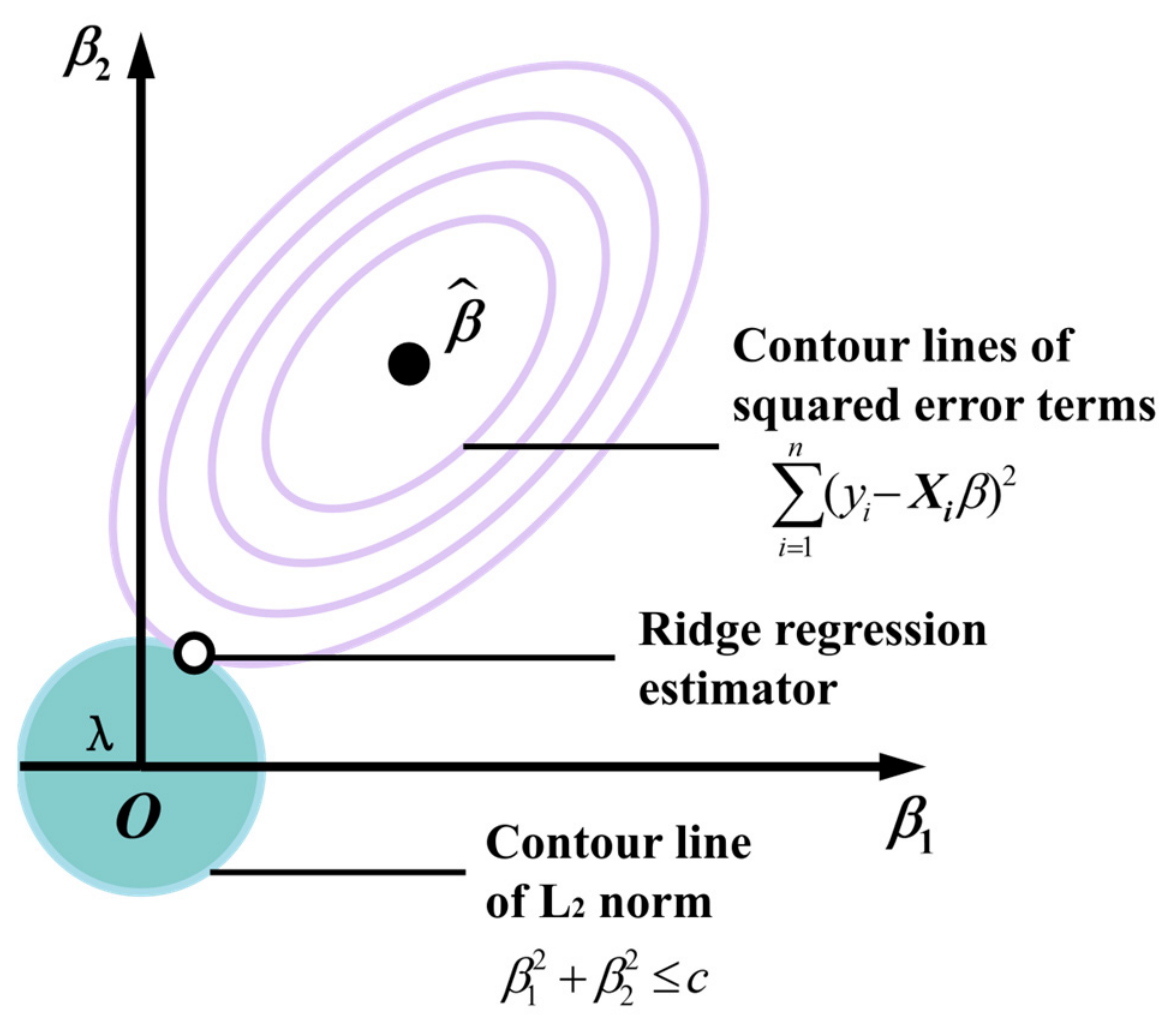
Figure 2 shows the schematic principle of ridge regression. In two-dimensional parameter space $\left({\mathit{\beta }}_1,{\mathit{\beta }}_2\right)$, concentric ellipses denote contours of residual sum of squares, and their center corresponds to the theoretical optimal solution of ordinary least squares. The circular area represents L2 norm constraint, where constraint radius c has negative correlation with regularization parameter $\lambda$. It seeks the parameter combination with minimum error inside the constraint region. Its optimal solution lies the tangent point of error contours and the constraint circle, effectively lowering parameter sensitivity to noise.

The hybrid model proposed in this paper takes IMF component features decomposed by EEMD as input. The low-frequency component of seepage pressure mainly shows long-term evolution and a gradually changing linear trend. If a complex nonlinear model is used for fitting, overfitting may occur. By contrast, ridge regression features a simple structure and high computational efficiency. This method can accurately capture the long-term linear evolution of seepage pressure, suppress model oscillation caused by multicollinear driving factors, and guarantee stable prediction of low-frequency components. This is the core reason why ridge regression is selected in this study.

2.4. Hybrid Transformer–BiLSTM Model and Multivariate Fusion Layer

The vanilla Transformer with the attention mechanism was proposed by the Google team in 2017 [33]. Graves and Schmidhuber built the bidirectional time-series modeling framework of BiLSTM based on LSTM in 2005 [34]. Both architectures possess unique structural advantages for nonlinear time-series prediction [35,36]. This work applies a multi-scale differentiated modeling scheme to EEMD-decomposed IMF components. The Transformer BiLSTM hybrid model fits medium- and high-frequency seepage pressure components controlled by coupled factors—reservoir water level fluctuation, rainfall infiltration and periodic temperature change—which hold intricate nonlinear temporal relations and lag influences. In comparison, ridge regression handles low-frequency components governed by long-term time-related evolution and mild linear trends. Parallel dynamic tuning of the two models captures full seepage pressure characteristics.

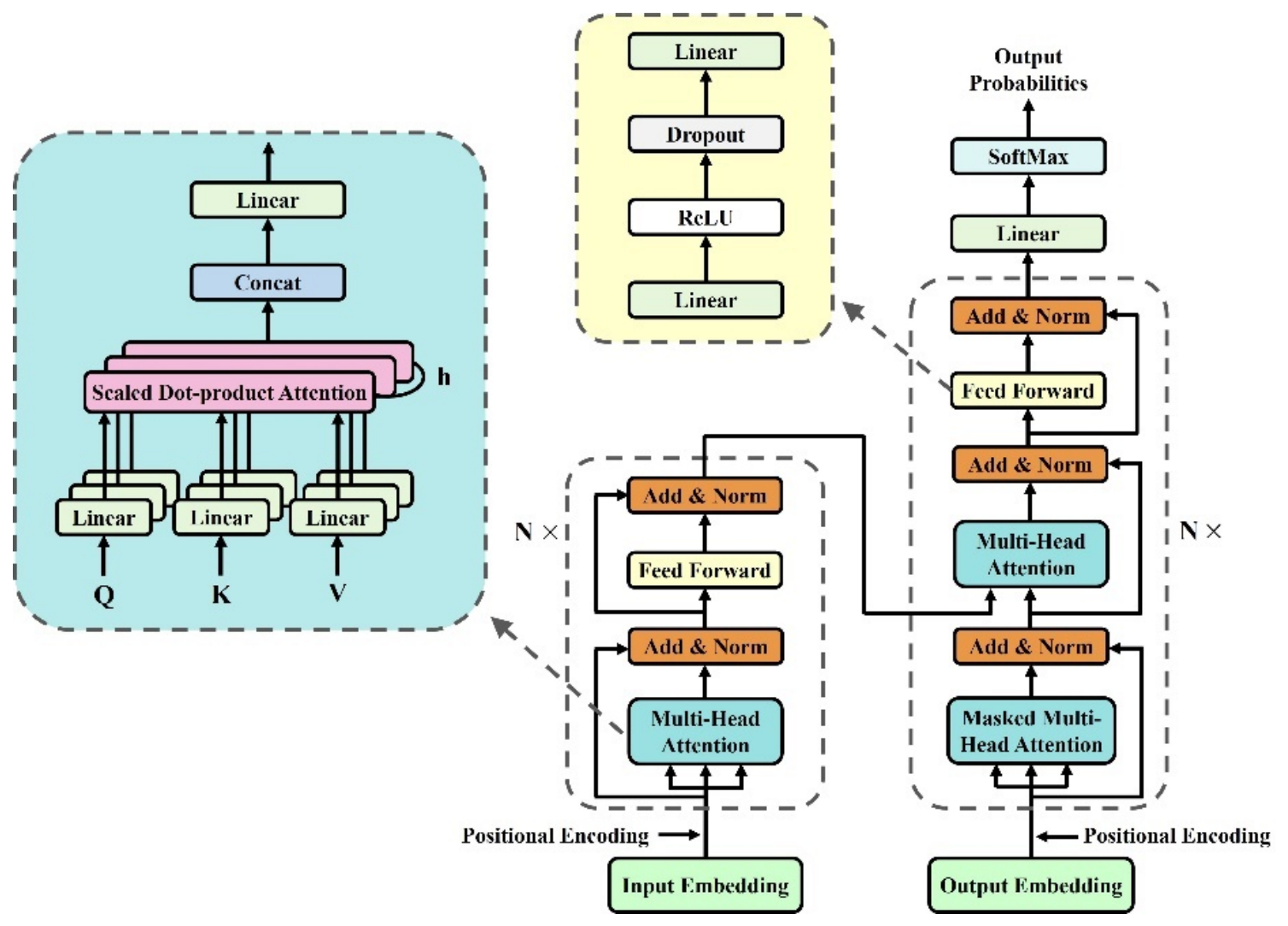
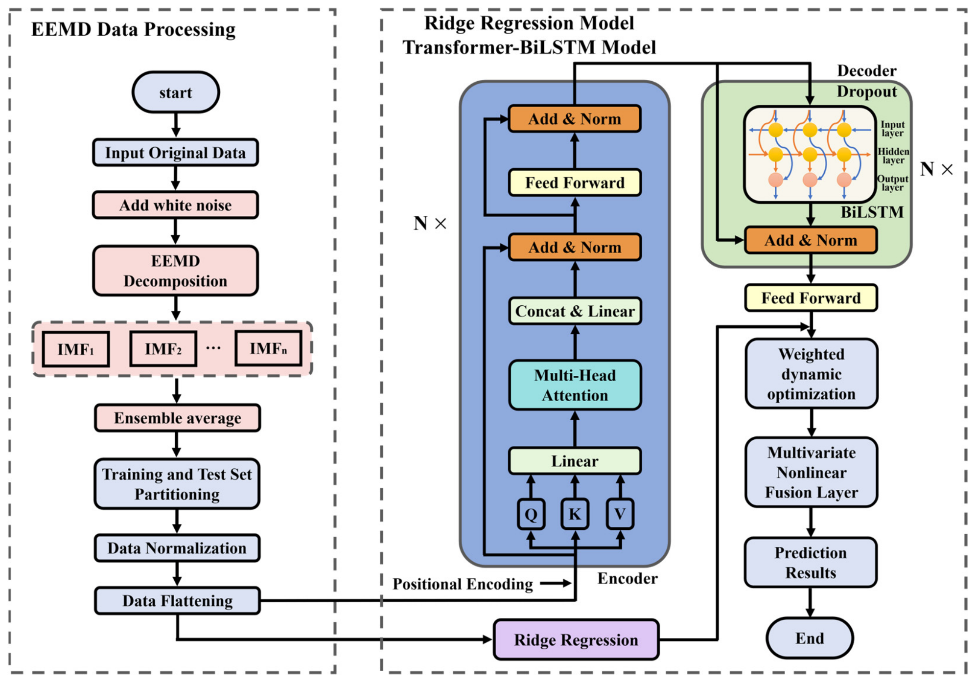
Transformer serves as the core module for capturing long-range correlations in time-series features, and its architecture is displayed in Figure 3. Seepage pressure responses of concrete dams exhibit prominent lag characteristics. The impacts of upstream water level variation and rainfall infiltration propagate gradually through fractured foundation rock masses and persist in the seepage field over timescales ranging from several days to dozens of days. Conventional recurrent time-series models suffer from gradient vanishing, which restricts their capacity to capture long-range dependencies. The multi-head self-attention mechanism dynamically assigns attention weights to features at different timestamps via matrix operations. It can autonomously quantify the influence intensity of historical loads on current seepage pressure and address the issue of long-term lag effects. The calculation formula is given as

$$\begin{array}{l}MultiHead(\mathit{Q},\mathit{K},\mathit{V})\\ =Concat(hea{d}_1,\dots ,hea{d}_h){\mathit{W}}^{\mathit{O}}\end{array}$$

(10)

$$\begin{array}{cc}\hfill {head}_i& =Attention(\mathit{Q}{\mathit{W}}_{\mathit{i}}^{\mathit{Q}},\mathit{K}{\mathit{W}}_{\mathit{i}}^{\mathit{K}},\mathit{V}{\mathit{W}}_{\mathit{i}}^{\mathit{V}})\hfill \\ & =Softmax({\displaystyle \frac{\mathit{Q}{\mathit{W}}_{\mathit{i}}^{\mathit{Q}}{(\mathit{K}{\mathit{W}}_{\mathit{i}}^{\mathit{K}})}^T}{\sqrt{d_k}}})\mathit{V}{\mathit{W}}_{\mathit{i}}^{\mathit{V}}\hfill \end{array}$$

(11)

where $\mathit{Q},\mathit{K},\mathit{V}$ are the query, key and value matrices, h is the number of attention heads, ${\mathit{W}}_{\mathit{i}}^{\mathit{Q}},{\mathit{W}}_{\mathit{i}}^{\mathit{K}},{\mathit{W}}_{\mathit{i}}^{\mathit{V}},{\mathit{W}}^{\mathit{O}}$ are the learnable parameter matrices, and $d_k$ is the dimension of each key vector. The self-attention mechanism itself does not contain temporal position information and cannot perceive the sequence’s order, while the evolution of pressure has strict temporal causality. Hence, sine and cosine functions are introduced to generate positional encoding, which embeds timestamp positional information into feature vectors:

$$P{E}_{(pos,2i)}=\sin ({\displaystyle \frac{pos}{{10000}^{2i/d_{model}}}})$$

(12)

$$P{E}_{(pos,2i+1)}=\cos ({\displaystyle \frac{pos}{{10000}^{2i/d_{model}}}})$$

(13)

where pos is the position of the input feature factor within the sequence; i is the index of the input feature factor; and $d_{model}$ is the dimension of input feature factors. Sine functions encode even indices, while cosine functions encode odd indices.

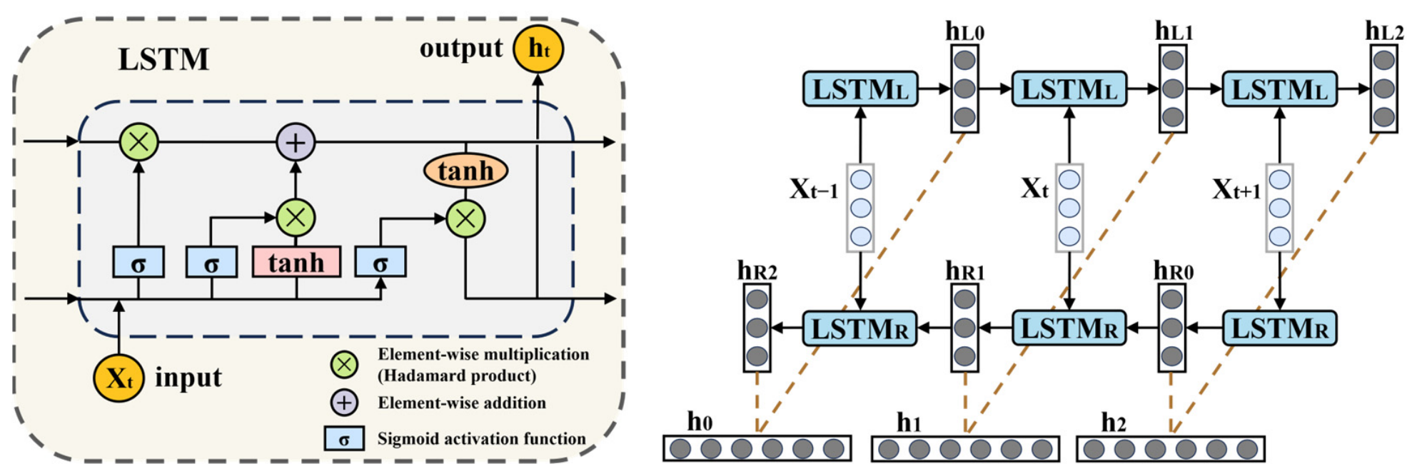
After Transformer extracts long-range global correlation features, BiLSTM is introduced to mine bidirectional local temporal dependencies of the sequence, with its architecture illustrated in Figure 4. Standard LSTM retains and updates temporal information via gate control mechanisms including input gate, forget gate and output gate. It addresses the gradient vanishing issue of conventional recurrent neural networks, highlights lag effects in seepage pressure series, and restores the gradual response law of seepage pressure during reservoir water level fluctuation. BiLSTM is a bidirectional stacked structure composed of parallel forward and backward LSTM units. Its hidden states are concatenated at each timestamp to form bidirectional temporal features. The state update formulas are expressed as

$$\overrightarrow{{\mathit{h}}_{\mathit{t}}}=LSTM(x_t,\overrightarrow{{\mathit{h}}_{\mathit{t}-1}})$$

(14)

$$\overleftarrow{{\mathit{h}}_{\mathit{t}}}=LSTM(x_t,\overleftarrow{{\mathit{h}}_{\mathit{t}+1}})$$

(15)

$${\mathit{h}}_{\mathit{t}}=[\overrightarrow{{\mathit{h}}_{\mathit{t}}};\overleftarrow{{\mathit{h}}_{\mathit{t}}}]$$

(16)

where $\overrightarrow{{\mathit{h}}_{\mathit{t}}},\overleftarrow{{\mathit{h}}_{\mathit{t}}}$ are the forward and backward hidden states and ${\mathit{h}}_{\mathit{t}}$ represents the concatenated bidirectional features that fully preserve contextual information of the sequence. Compared with single LSTM, BiLSTM simultaneously exploits historical and future temporal information to capture asymmetric fluctuation patterns of seepage pressure under working conditions such as sharp water level rise and heavy rainfall infiltration.

Seepage pressure IMF components first go through Transformer layers to extract long-range correlation features, then through BiLSTM layers to capture bidirectional temporal relations and generate training outputs via full connected layers. The existing Transformer has weak local sensitivity, LSTM suffers gradient decay for long dependencies, and Transformer–LSTM ignores backward information. The presented hybrid model builds a complementary structure that combines Transformer’s long-range dependency extraction ability and BiLSTM’s strength in nonlinear time-series fitting. Matching ridge regression to components of different scales eliminates fitting bias from single-model approaches improves computation speed and ensures stable prediction accuracy and model robustness.

After the parallel training and dynamic optimal selection of all IMF components, conventional decomposition–ensemble models rely on linear summation. Such methods fail to fully exploit nonlinear coupling among multi-scale components and lead to the loss of valid output information. To address this, the multi-scale fusion reconstruction layer proposed in this study realizes the deep integration of optimal training outputs and accurate reconstruction of the original seepage pressure sequence. The seepage pressure of concrete dams arises from coupled multi-scale physical processes. High-frequency random disturbances, medium-frequency periodic oscillations and low-frequency long-term trends do not follow simple linear superposition. Taking the optimal prediction sequence of each component as multivariate inputs, the fusion layer adaptively learns coupling relations across components of different frequencies through fully connected neural networks. It maximally retains valid information of trend and fluctuation terms decomposed by EEMD.

3. Integrated Prediction Method

3.1. Model Fusion Method

Concrete dam seepage pressure sequences feature strong nonlinearity, nonstationarity, multi-scale superposition and lag effects [37]. Existing models fail to fully capture multi factor coupling, mine nonlinear temporal relations and deliver clear physical interpretation [38]. To tackle these issues, this paper builds an innovative seepage pressure prediction model combining EEMD multi-scale preprocessing, parallel training and optimization of two models (ridge regression and Transformer–BiLSTM), and multivariate nonlinear fusion layer reconstruction. This model overcomes structural flaws of single models and uniform modeling drawbacks of conventional decomposition–ensemble frameworks, and forms a seepage prediction system with high precision, reliable robustness and good physical interpretability. The overall structure diagram of the model is shown in Figure 5.

All modules of the model operate in close synergy. EEMD serves as preprocessing to conduct adaptive multi-scale decomposition on cleaned raw seepage pressure series, decoupling nonstationary data into three IMF categories for differentiated modeling: high-frequency random noise and instantaneous disturbances, medium-frequency environmental load responses, and low-frequency long-term time-dependent evolution trends. This step reduces data-level modeling difficulty and improves component interpretability by providing structured inputs. Subsequently, a dual-model parallel training and optimization architecture is built based on component characteristics. For low-frequency components dominated by gentle linear trends with severe collinearity among driving factors, ridge regression eliminates multicollinearity induced by multi-order lagged water level terms and time-dependent factors during linear fitting. For medium- and high-frequency components driven by factors including reservoir water level fluctuation, periodic temperature variation, and rainfall infiltration—which feature strong nonlinearity and remarkable lag effects—Transformer–BiLSTM utilizes multi-head self-attention and bidirectional temporal mining capacity by replacing the decoder inside the Transformer with BiLSTM. After parallel dual-model training for each component, comprehensive optimization metrics based on fundamental indicators are constructed to select optimal outputs. These optimal results are fed into the multivariate nonlinear fusion reconstruction layer, where fully connected networks adaptively extract relationships among components, integrate features and conduct dimension mapping, and finally reconstruct the global prediction series of concrete dam seepage pressure. All modules are elaborately designed targeting evolution characteristics of dam seepage pressure and deeply matched with seepage physical mechanisms, thus guaranteeing prediction accuracy and objectivity of the model.

3.2. Model Evaluation Metrics

To comprehensively evaluate model prediction accuracy, four metrics are adopted: root mean square error (RMSE), mean absolute error (MAE), mean absolute percentage error (MAPE) and coefficient of determination (R²). Their formulas are given as follows:

$$\mathrm{RMSE}=\sqrt{{\displaystyle \frac{1}{n}}{\displaystyle \sum _{i=1}^n{\left(y_{true,i}-y_{pred,i}\right)}^2}}$$

(17)

$$\mathrm{MAE}={\displaystyle \frac{1}{n}}{\displaystyle \sum _{i=1}^n\left|y_{true,i}-y_{pred,i}\right|}$$

(18)

$$\mathrm{MAPE}={\displaystyle \frac{100\%}{n}}{\displaystyle \sum _{i=1}^n\left|\frac{y_{true,i}-y_{pred,i}}{y_{true,i}}\right|}$$

(19)

$${\mathrm{R}}^2=1-{\displaystyle \frac{{\displaystyle \sum _{i=1}^n{\left(y_{true,i}-y_{pred,i}\right)}^2}}{{\displaystyle \sum _{i=1}^n{\left(y_{true,i}-{\overline{y}}_{true}\right)}^2}}}$$

(20)

where $y_{true,i}$ is the measured actual monitoring value, $y_{pred,i}$ is the predicted value, and ${\overline{y}}_{true}$ is the mean of actual measured values.

Given the parallel dual-model strategy used herein, the four evaluation metrics often produce inconsistent rankings that hinder optimal model selection. To resolve one-sided evaluation, dimensional inhomogeneity and unbalanced tradeoffs between error and fitting performance, this study develops a normalized Comprehensive Optimal Index (COI) tailored to dam engineering demands. The index normalizes and weight-fuses the four metrics to remove dimensional differences, enabling quantitative, objective model screening.

3.2.1. Normalization of Indicators

RMSE, MAE, MAPE and R² differ drastically in dimension, value range and variation trend. Normalization is first performed on all metrics to achieve comparability.

For error metrics (RMSE, MAE, MAPE), where smaller values indicate better performance, reverse normalization is adopted to calculate the evaluation score $S_i\in [0,1]$. The value closer to 1 stands for superior model performance:

$$S_i={\displaystyle \frac{X_{\max }-X}{X_{\max }-X_{\min }}}$$

(21)

where X is the raw metric value of the evaluated model, and $X_{\max },X_{\min }$ are the maximum and minimum raw values of this error metric across all candidate models for component optimization.

For goodness-of-fit metrics such as R², where larger values correspond to better fitting performance, forward normalization is used to compute the evaluation score $S_{{\mathrm{R}}^2}\in [0,1]$. The value closer to 1 signifies more satisfactory fitting results:

$$S_{{\mathrm{R}}^2}={\displaystyle \frac{X_{{\mathrm{R}}^2}-X_{{\mathrm{R}}^2\left(\min \right)}}{X_{{\mathrm{R}}^2(\max )}-X_{{\mathrm{R}}^2\left(\min \right)}}}$$

(22)

where $X_{{\mathrm{R}}^2}$ is the raw R² value of the evaluated model and $X_{{\mathrm{R}}^2(\max )},X_{{\mathrm{R}}^2\left(\min \right)}$ are the maximum and minimum R² values of all candidate models for component optimization.

3.2.2. Construction of Comprehensive Optimal Indicators

Based on normalized scores, differentiated weights are assigned to each normalized metric considering the engineering seepage characteristics of concrete dams and metric representativeness, subject to $\Sigma \omega =1$. The core of dam deformation prediction resides in a hierarchical paradigm that prioritizes, first, the characterization of long-term structural trends; second, the mitigation of short-term abrupt anomaly risks; and third, the assurance of predictive accuracy under routine steady-state operating conditions. R², the core metric reflecting overall model fitting performance, is assigned the maximum weight. RMSE, sensitive to large errors and capable of capturing global prediction bias, receives the second highest weight. MAE and MAPE, which characterize average accuracy from absolute and relative error perspectives respectively, share identical weights. Weight coefficients can be flexibly adjusted according to dam type and prediction scenarios, granting favorable engineering scalability.

COI is the weighted sum of the scores of each normalized indicator:

$$COI={\omega }_{\mathrm{RMSE}}{S}_{\mathrm{RMSE}}+{\omega }_{\mathrm{MAE}}{S}_{\mathrm{MAE}}+{\omega }_{\mathrm{MAPE}}{S}_{\mathrm{MAPE}}+{\omega }_{{\mathrm{R}}^2}{S}_{{\mathrm{R}}^2}$$

(23)

where $COI\in \left[0,1\right]$, with larger values indicating superior model performance.

For each individual IMF component decomposed by EEMD, the COI values of ridge regression and Transformer–BiLSTM are separately calculated as $CO{I}_{Ridge}$ and $CO{I}_{TB}$:

• If $CO{I}_{Ridge}>CO{I}_{TB}$, ridge regression outputs serve as component optima;
• If $CO{I}_{Ridge}<CO{I}_{TB}$, Transformer–BiLSTM outputs are adopted instead;
• If $CO{I}_{Ridge}=CO{I}_{TB}$, pick faster model to balance cost and accuracy.

The COI realizes quantitative fusion of multiple evaluation metrics and eliminates one-sided judgment caused by single indicators. It enhances objectivity and repeatability of dual-model parallel optimization, laying a high-precision training foundation.

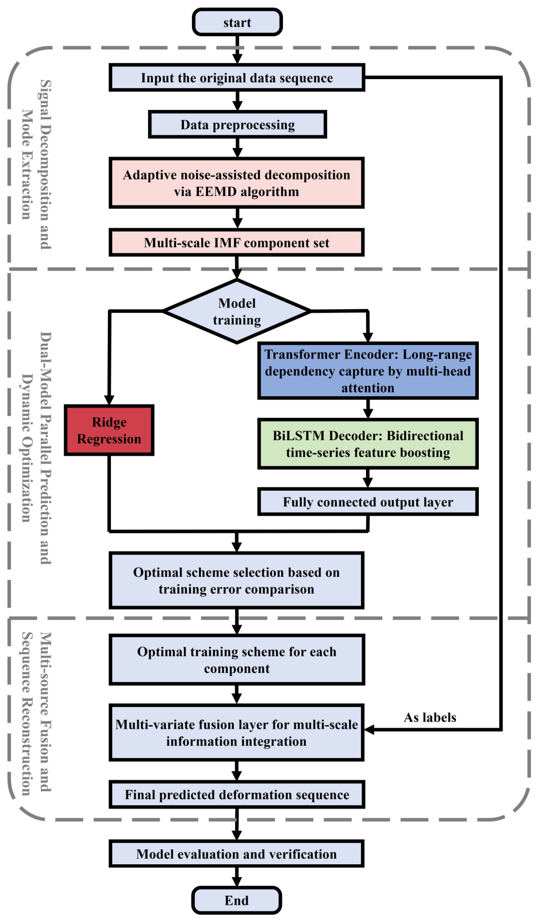
3.3. Overall Process

The overall workflow of the proposed concrete dam seepage pressure prediction method is illustrated in Figure 6, detailed as follows:

(1) Signal Decomposition and Mode Extraction

Raw time series undergo cleaning, outlier removal and missing value filling. EEMD adaptively decomposes processed seepage data into multi-scale IMFs. Invalid physically meaningless components are removed after validity test, and valid IMFs are grouped by frequency: high-frequency random noise/rainfall disturbance, medium-frequency environmental load-induced seepage responses, low-frequency long-term trend terms of foundation and impervious curtain evolution, providing structured inputs.

(2) Dual-Model Parallel Training and Dynamic Optimization

Ridge regression and Transformer–BiLSTM are trained in parallel for frequency-varying components. Ridge regression removes multicollinearity via L2 regularization to fit long-term linear trends. Transformer–BiLSTM utilizes multi-head attention and bidirectional BiLSTM to capture complex nonstationary medium–high frequency lagged fluctuations. The COI synthesizes normalized weighted metrics to pick optimal outputs.

(3) Multivariate Fusion and Series Reconstruction

Optimal component predictions are concatenated into multi-dimensional features. A nonlinear fusion layer learns feature mapping to raw series, extracts global temporal dependencies, integrates features and maps dimensions to reconstruct full seepage pressure prediction series.

(4) Model Evaluation and Validation

Global prediction results are post-processed and optimized. Model performance is evaluated via visualization and quantitative metrics. Field monitoring data verify model reliability and adaptability, supporting dam seepage safety monitoring and early warning.

4. Case Study

4.1. Overview of the Project

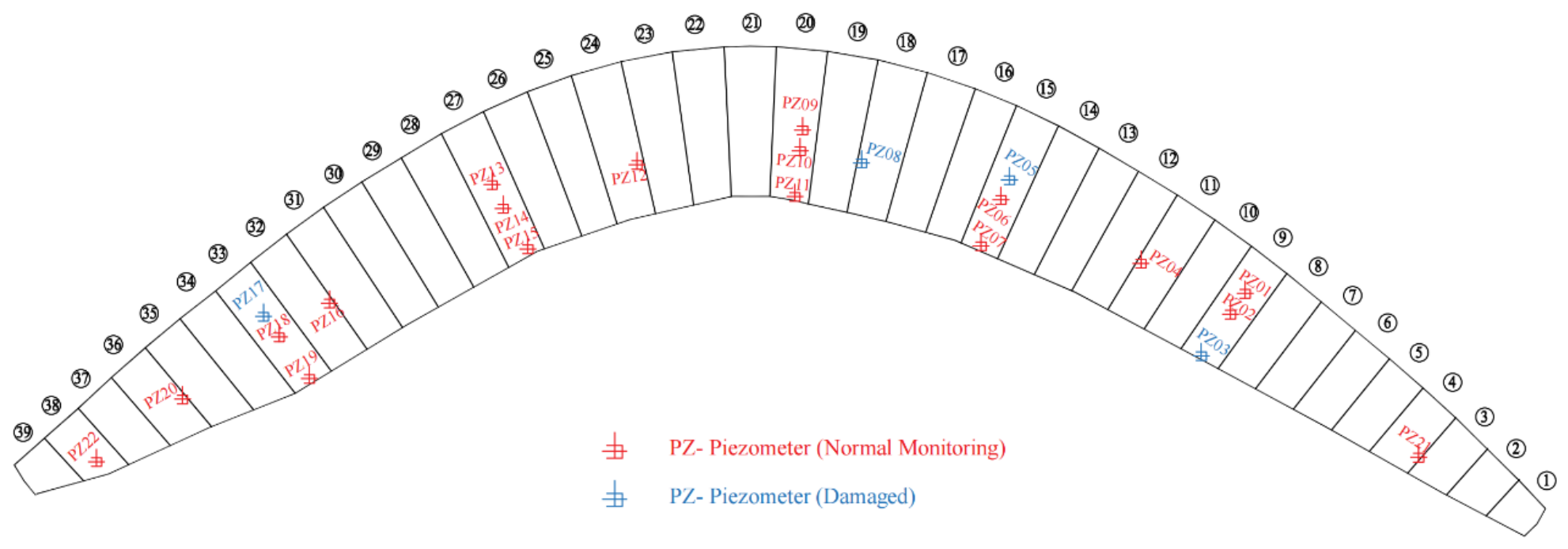
A concrete double-curvature arch dam of a hydropower station—which is in Panzhihua, Sichuan, China—is taken as the engineering case. As a landmark hydraulic hub for cascade exploitation along the Yalong River, it features a large-scale and complex service environment. A long-term safety monitoring system covering environmental factors, seepage pressure and temperature has been deployed, among which dam seepage monitoring acts as a core item. The continuous and representative data series can reflect the seepage evolution of high arch dams under multi-field coupling.

Layout of its seepage pressure monitoring points is displayed in Figure 7. The complete seepage monitoring system arranges 18 functional piezometers and seepage flow sensors around the foundation anti-seepage curtain, key dam sections, and two abutments, with automatic acquisition for long-term continuous observation. Long-term seepage records from typical monitoring sections form the core dataset for investigating the coupled impacts of water level fluctuation, temperature variation and time-dependent deformation on foundation seepage pressure, and verify the practicability of the proposed multi-scale fusion prediction model for concrete dam seepage pressure monitoring.

4.2. Dataset Selection

Per the statistical models in Section 2.1, dam seepage pressure is controlled by upstream/downstream water levels, rainfall infiltration, periodic temperature and long-term aging, with spatiotemporal correlations across monitoring points. This paper selects the measured data from 2010 to 2019 for research, with a sampling interval of 12 h. Inputs cover reservoir level, downstream stage, rainfall, temperature, time and piezometric head. Auxiliary data are resampled to match seepage timestamps to unify time axes and remove temporal offset. Factor components are formulated as

$$\left\{\begin{array}{c}{H}_h=\left\{h_1,\overline{h_{2~4}},\overline{h_{5~15}},\overline{h_{16~30}},\overline{h_{31~60}},\overline{h_{61~100}}\right\}\hfill \\ H_p=\left\{p_1,\overline{p_{2~4}},\overline{p_{5~8}}\right\}\hfill \\ H_t=\left\{\sin {\displaystyle \frac{2\mathsf{\pi }it}{365}},\cos {\displaystyle \frac{2\mathsf{\pi }it}{365}} \right\},i=1,2\hfill \\ H_{\theta }=\left\{\theta ,ln\theta \right\},\theta =t/100\hfill \end{array}\right.$$

(24)

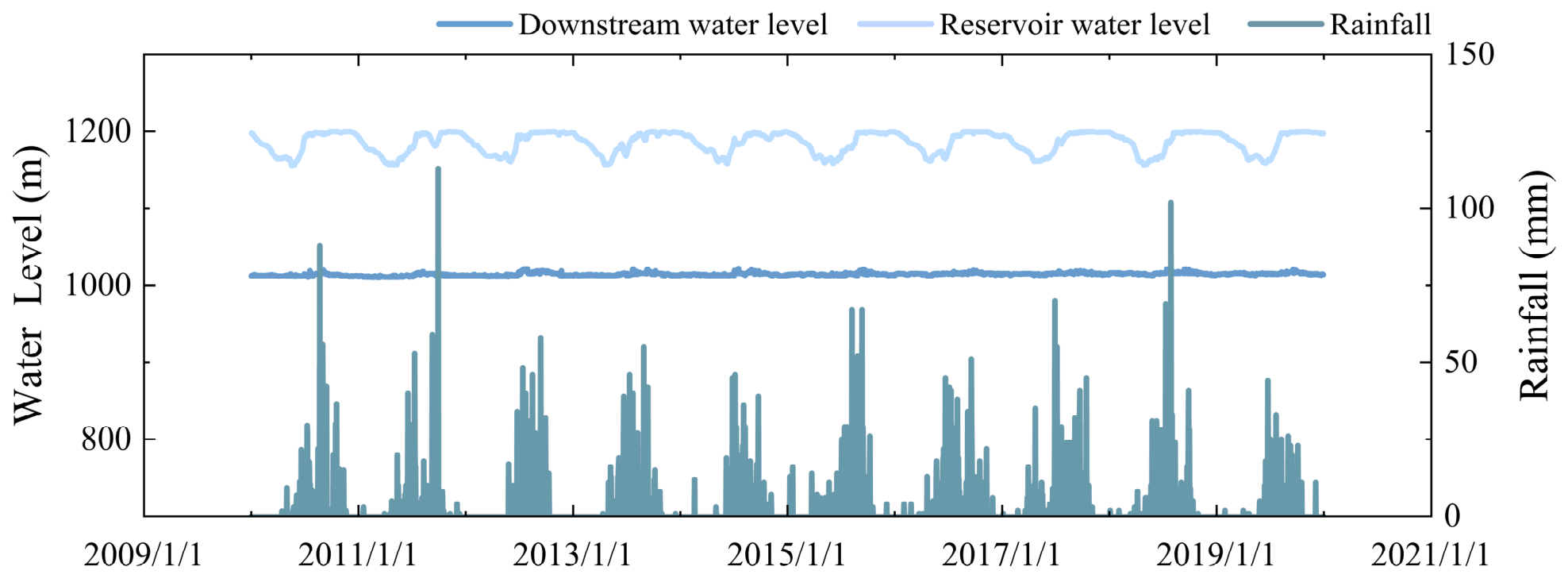
After time synchronization, 7302 valid data groups are obtained. The historical curves of water level and rainfall over the monitoring period are plotted in Figure 8. The complete, high-quality dataset spans full hydrological cycles with obvious dry (Dec.–Apr.) and flood (Jul.–Oct.) seasons, covering routine reservoir operating levels and offering representative temporal features.

4.3. Model Parameter Settings

The prediction experiments are conducted under a single-step rolling prediction framework. In engineering practice, single-step rolling prediction enables real-time model refreshing and guarantees that each forecast is conditioned on the most recent system state, thereby avoiding the error accumulation and uncertainty propagation inherent in multi-step direct forecasting. Furthermore, because concrete dam seepage early-warning systems rely on instantaneous threshold exceedance triggers, the high accuracy and low latency of single-step rolling outputs are essential for reliable anomaly detection and rapid emergency response.

For each monitoring point, the first 75% of seepage pressure data over the monitoring period are taken as the training set and the remaining 25% as the test set. Targeted parameter tuning based on dam seepage pressure characteristics and model performance requirements yields the optimal model, with results shown in

Table 1. Model hyperparameter selection.

Module Name	Parameter	Value
Data Preprocessing and EEMD	Sliding window length	90
	EEMD noise amplitude	0.001
	EEMD ensemble size	200
Transformer	Number of encoder layers	6
	Number of multi-head attention heads	8
	Self-attention feature dimension	256
BiLSTM	Number of network layers	4
	Number of neurons per layer	256
	Learning rate	0.0005
Training and Regularization Parameters	Dropout rate	0.3
	L2 regularization coefficient	0.001
	Maximum training epochs	100
Prediction Settings	Prediction horizon (steps)	1 step (12 h; 0.5 d)

.

To ensure the accuracy of ablation experiments, identical hyperparameter configurations are applied to all models. All experiments are developed in Python 3.9.18 and Spyder 5.4.3, with PyTorch 2.5.0 employed as the deep learning framework for standardization.

4.4. EEMD Data Preprocessing

To verify multi-scale decomposition adaptability and model generalization, four monitoring points (PZ01, PZ09, PZ10, PZ15) are selected by dam foundation seepage zoning and monitoring layout. PZ01 (right bank) and PZ09 (mid-riverbed) behind the impervious curtain reflect upstream seepage evolution. PZ10 in the drainage zone captures drainage regulated responses, and PZ15 at the downstream left bank toe reflects seepage pressure after multi-stage attenuation. Covering three sections and functional seepage zones, they characterize multi region evolution of the dam foundation seepage field.

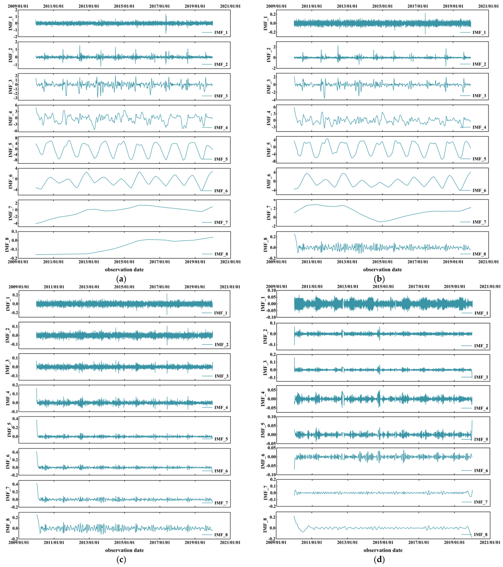
Missing and anomalous raw data are corrected by linear interpolation. EEMD is applied to decompose seepage pressure series into eight intrinsic mode function (IMF) components, which are categorized into high-frequency, medium-frequency and low-frequency trend components. The IMFs charts are shown in Figure 9.

EEMD results match well with seepage zoning patterns. For PZ01 and PZ09 behind the impervious curtain, overall pressure amplitude is high with prominent medium-frequency components. IMF4 to IMF6 exhibit clear monthly oscillation patterns, confirming the dominant driving effect of reservoir-level cycles on seepage pressure behind the curtain. PZ01 shows a slow upward trend, while riverbed PZ09 features a long-term downward trend, reflecting spatial disparities in anti-seepage system performance across sections. For PZ10 in the drainage zone, pressure amplitude is far lower than behind the curtain, with a notably increased share of high-frequency components. IMF1 to IMF5 present dense micro-amplitude high-frequency oscillations, indicating drainage holes attenuate seepage pressure head and smooth periodic seepage fluctuations. PZ15 near the dam toe has the lowest pressure amplitude among all points. All its components are dominated by high-frequency micro fluctuations, suggesting the dam toe seepage field has stabilized after multi-stage regulation, with fluctuations mainly from monitoring noise and local flow disturbances.

4.5. Analysis of Prediction Accuracy

Seepage pressure amplitudes differ significantly across spatial zones. Seepage heads are high behind the impervious curtain and decline progressively in the dam foundation drainage zone and at the dam toe. As a single evaluation index cannot fully reflect the overall prediction performance, a new comprehensive optimization index (COI) is proposed in this paper.

This study engaged five senior experts in the field of hydraulic structure safety monitoring, comprising two professor-level senior engineers from universities, two chief engineers from river basin operation and management agencies, and one deputy chief engineer from a design institute. A modified Delphi method combined with the Analytic Hierarchy Process (AHP) was employed to conduct pairwise importance comparisons among the four metrics—RMSE, MAE, MAPE, and R². Through validation against engineering cases and expert scoring, an initial weight vector was derived: ${\omega }_{\mathrm{RMSE}}=0.283$, ${\omega }_{\mathrm{MAE}}=0.172$, ${\omega }_{\mathrm{MAPE}}=0.165$, and ${\omega }_{{\mathrm{R}}^2}=0.380$. The experts unanimously concurred that the goodness-of-fit for long-term trends constitutes the primary criterion in concrete dam safety assessment, warranting an R² weight proportion approaching 40%. RMSE, serving as a global error metric sensitive to large deviations, possesses higher engineering sensitivity than average error metrics and thus should be assigned a weight significantly exceeding those of MAE and MAPE. MAE and MAPE characterize average accuracy from absolute and relative perspectives, respectively; they are informationally complementary and of equivalent importance. Consistency testing yielded a consistency ratio (CR) of 0.062 for the judgment matrix, satisfying the threshold CR < 0.10; the matrix therefore passed the consistency test, confirming the absence of logical conflicts in the expert judgments.

Considering that the research object operates predominantly under steady non-flood-season conditions throughout most of the year and exhibits a relatively low proportion of samples with extreme abrupt seepage pressure changes, minor engineering adaptive rounding was applied to the original weights. Specifically, the R² weight was adjusted upward from 0.380 to 0.40 to further consolidate the dominance of long-term trend evaluation. The RMSE weight was trimmed from 0.283 to 0.30 without further elevation, thereby preventing excessive penalization of minor normal fluctuations. The MAE and MAPE weights were synchronously reduced from 0.172 and 0.165, respectively, and rounded to 0.15, preserving their equal status; their combined weight of 0.30 effectively discriminates average accuracy differences among candidate models under steady operating conditions. Verification confirms that the adjusted weights sum strictly to unity, satisfying the normalization constraint requisite for weighted comprehensive evaluation. The final weight configuration is ${\omega }_{\mathrm{RMSE}}=0.30$, ${\omega }_{\mathrm{MAE}}=0.15$, ${\omega }_{\mathrm{MAPE}}=0.15$, ${\omega }_{{\mathrm{R}}^2}=0.40$. The COI is established via weighted summation:

$$COI=0.30S_{\mathrm{RMSE}}+0.15S_{\mathrm{MAE}}+0.15S_{\mathrm{MAPE}}+0.40S_{{\mathrm{R}}^2}$$

(25)

In order to better quantify the training effectiveness of each model for different IMF components, taking monitoring point PZ01 as an example, the core evaluation indices and COI values of eight IMF components trained by ridge regression and Transformer–BiLSTM are summarized in

Table 2. Training evaluation indexes of IMF components for measuring point PZ01.

Component	Model	R2	${\mathit{S}}_{{\mathbf{R}}^2}$	RMSE (m)	${\mathit{S}}_{\mathbf{RMSE}}$	MAE (m)	${\mathit{S}}_{\mathbf{MAE}}$	MAPE (%)	${\mathit{S}}_{\mathbf{MAPE}}$	COI
IMF1 (High-frequency)	Ridge Regression	0.7215	0.0000	0.4231	0.6205	0.3422	0.6138	18.76	0.0000	0.2782
	Transformer–BiLSTM	0.9842	0.9542	0.0753	0.9382	0.0587	0.9395	3.091	0.8898	0.9375
IMF2 (High-frequency)	Ridge Regression	0.7483	0.0973	0.4512	0.5948	0.3601	0.5932	17.23	0.0869	0.3194
	Transformer–BiLSTM	0.9867	0.9633	0.0682	0.9447	0.0534	0.9455	2.682	0.9131	0.9475
IMF3 (High-frequency)	Ridge Regression	0.8126	0.3309	0.7015	0.3662	0.5623	0.3609	12.54	0.3532	0.3493
	Transformer–BiLSTM	0.9879	0.9677	0.1824	0.8404	0.1432	0.8424	2.970	0.8966	0.9000
IMF4 (Medium-frequency)	Ridge Regression	0.8754	0.5590	0.9327	0.1549	0.7486	0.1469	9.649	0.5173	0.3697
	Transformer–BiLSTM	0.9913	0.9800	0.2105	0.8147	0.1637	0.8188	2.041	0.9495	0.9017
IMF5 (Medium-frequency)	Ridge Regression	0.9187	0.7163	1.1023	0.0000	0.8765	0.0000	7.778	0.6235	0.3800
	Transformer–BiLSTM	0.9942	0.9906	0.2486	0.7799	0.1923	0.7860	1.646	0.9716	0.8938
IMF6 (Medium-frequency)	Ridge Regression	0.9472	0.8198	0.5234	0.5289	0.4125	0.5330	5.621	0.7462	0.6785
	Transformer–BiLSTM	0.9876	0.9666	0.2297	0.7972	0.1802	0.7999	2.430	0.9273	0.8849
IMF7 (Low-frequency)	Ridge Regression	0.9925	0.9844	0.1176	0.8996	0.0918	0.9014	1.822	0.9620	0.9432
	Transformer–BiLSTM	0.9753	0.9219	0.2553	0.7738	0.2041	0.7724	4.181	0.8279	0.8409
IMF8 (Low-frequency)	Ridge Regression	0.9968	1.0000	0.0077	1.0000	0.0060	1.0000	1.146	1.0000	1.0000
	Transformer–BiLSTM	0.9702	0.9034	0.0215	0.9874	0.0174	0.9869	3.591	0.8614	0.9348

to quantify the training performance of each model on different IMF components. As shown, for high-frequency (IMF1–3) and medium-frequency (IMF4–6) components, the Transformer–BiLSTM model maintains R² above 0.98, yields far lower RMSE, MAE and MAPE than ridge regression and achieves significantly higher COI values. This demonstrates the model’s precise capture of nonlinear temporal dependencies, consistent with the physical mechanism of medium–high frequency seepage responses. For low-frequency components (IMF7–8), ridge regression presents prominent advantages. Its R² exceeds 0.99, error indices decrease markedly, and COI values all exceed 0.94. Compared with Transformer–BiLSTM, ridge regression effectively suppresses multicollinearity among seepage driving factors, enabling stable fitting of the long-term temporal evolution trend of dam foundation seepage pressure. The COI results align well with component frequency features, verifying both the effectiveness of the COI for dynamic dual-model selection and the scientific rationality of the multi-scale differentiated modeling strategy.

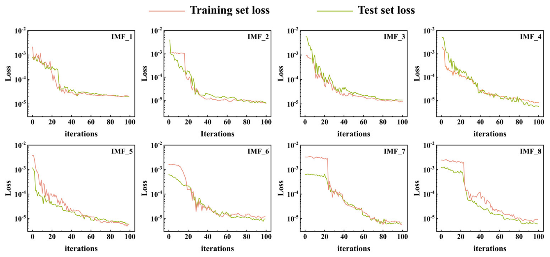
To verify the training stability and convergence speed of the proposed model, the training process of IMF components at point PZ01 is tracked, and the loss curves of the training and test sets against iteration number are presented in Figure 10. All IMF components converge rapidly in the early training phase and stabilize thereafter. The high-frequency IMF components (IMF1–3) achieve the fastest convergence, reaching a low loss level within only 20–30 iterations. This aligns with the physical nature of high-frequency components, having readily captured fluctuation patterns. The medium-frequency IMF components (IMF4–6) converge at a moderate rate, requiring around 40 iterations. These components correspond to seepage pressure responses driven by reservoir-level fluctuations and periodic temperature variations. Their hysteresis conduction effects and nonlinear multi-factor coupling demand more iterations to be fully characterized. The low-frequency IMF components (IMF7–8) exhibit the slowest convergence. Their temporal features reflect the long-term evolution trend of the dam foundation seepage field, involving gradual processes, thus necessitating sufficient iterations for accurate long-term trend fitting. Furthermore, the minor discrepancy between training and test set losses indicates no significant overfitting. This confirms that the EEMD multi-scale preprocessing and differentiated modeling strategy enable the model to capture seepage pressure evolution characteristics while maintaining favorable generalization ability. The overall model converges within approximately 80 iterations with high computational efficiency.

The proposed seepage pressure prediction model accurately reproduces the evolutionary trend of dam foundation seepage pressure, with the prediction metrics listed in

Table 3. Model prediction evaluation indicators for measuring points.

PZ01					PZ09
Indicators	R2	RMSE/m	MAE/m	MAPE/%	Indicators	R2	RMSE/m	MAE/m	MAPE/%
Training set	0.9928	0.7571	0.6922	2.3010	Training set	0.9983	0.2695	0.2122	0.5118
Test set	0.9902	0.8111	0.7033	3.1664	Test set	0.9969	0.3330	0.2432	0.6271
PZ10					PZ15
Indicators	R2	RMSE/m	MAE/m	MAPE/%	Indicators	R2	RMSE/m	MAE/m	MAPE/%
Training set	0.9955	0.1018	0.0812	0.5718	Training set	0.9935	0.0169	0.0138	0.8318
Test set	0.9915	0.0950	0.0769	0.6271	Test set	0.9884	0.0153	0.0108	0.5571

.

In terms of prediction performance, the proposed model outperforms single and traditional hybrid models in accuracy and stability. For PZ01, the training set respectively achieves an R² of 0.9928, with RMSE, MAE and MAPE of 0.7571 m, 0.6922 m and 2.3010%. The test set maintains a high R² of 0.9902 with controllable error growth, and the small performance gap between training and test sets indicates no significant overfitting. The predicted curve aligns well with measured seepage data. It reproduces the long-term evolution trend and finely captures short-term fluctuations induced by abrupt reservoir-level changes and heavy rainfall infiltration, overcoming limitations of traditional statistical models such as prediction lag and large local fitting errors under extreme conditions.

4.6. Comparison of Generalization Performance of Prediction Results

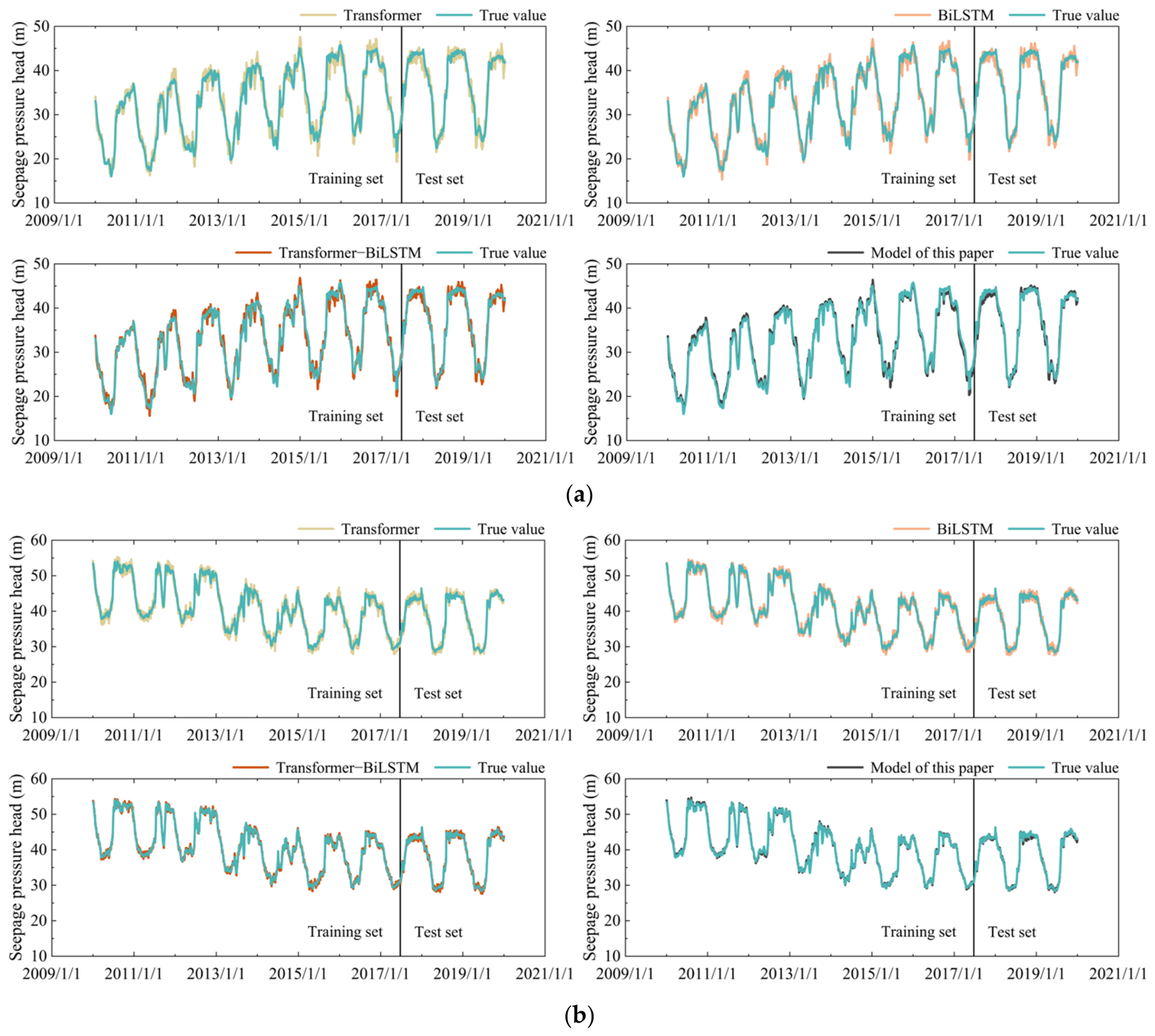
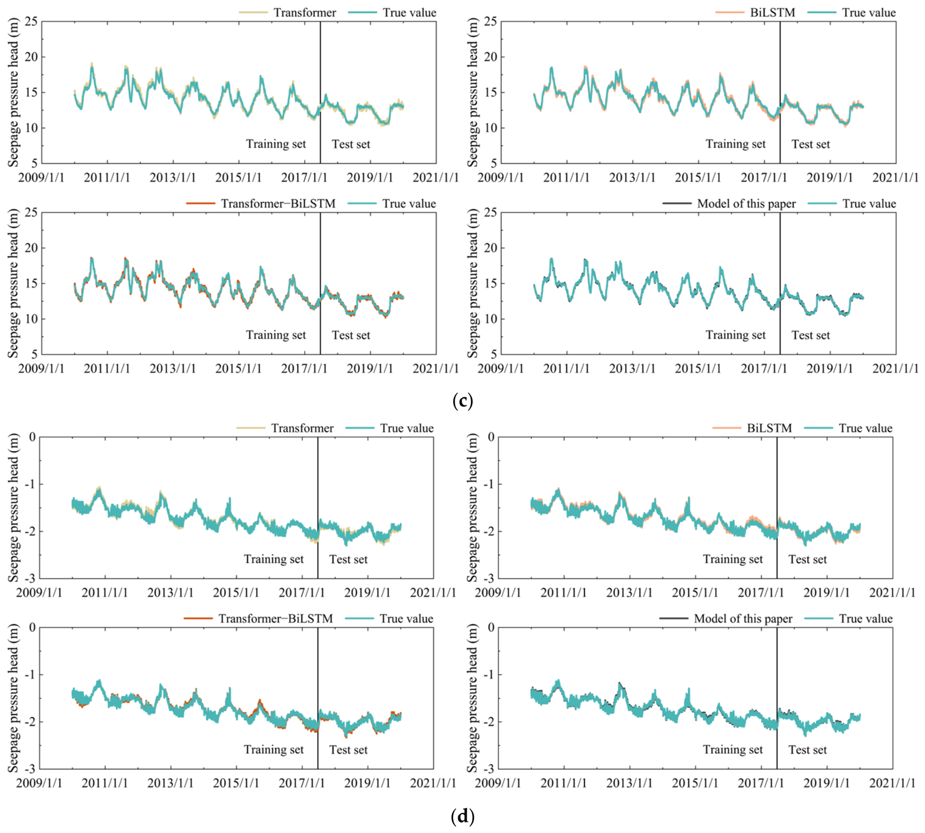
To verify the generalization and reliability of the proposed model for concrete dam seepage pressure prediction, its performance is compared with three benchmarks: Transformer, BiLSTM, and Transformer–BiLSTM. Typical monitoring points in three seepage functional zones (behind the anti-seepage curtain, dam foundation drainage zone, and dam toe) are analyzed. Comparisons of predicted seepage pressure head curves with measured data at the four points are presented in Figure 11.

As shown in Figure 11, the proposed seepage pressure prediction model based on multi-scale preprocessing and dual-model fusion delivers excellent performance across dam foundation regions with distinct seepage characteristics. For PZ01 and PZ09 behind the impervious curtain, seepage pressure heads feature high amplitudes and prominent annual periodic fluctuations driven by seasonal reservoir-level variations. The proposed model accurately reproduces the long-term evolution trend and annual fluctuation patterns, with far better agreement in amplitude and phase than the three benchmarks. It effectively mitigates the large deviation of Transformer at abrupt water level inflection points and the phase lag deficiency of BiLSTM. For PZ10 in the dam foundation drainage zone, regulated by drainage holes, seepage pressure heads decrease significantly, with an increased proportion of high-frequency small amplitude fluctuations. Benefiting from EEMD multi-scale decoupling, the proposed model outperforms benchmarks in capturing local fluctuation details and achieves higher local fitting accuracy. For PZ15 at the dam toe with low, stable seepage pressure, the model still maintains the minimum prediction deviation and reliably reflects the seepage field state. Experiments demonstrate that the proposed fusion model simultaneously achieves accurate long-term trend prediction and fine short-term fluctuation capture, exhibiting higher prediction accuracy and robustness across monitoring points in different seepage zones. The model matches the practical demands of dam seepage safety management well, with prediction errors far lower than those of the benchmarks.

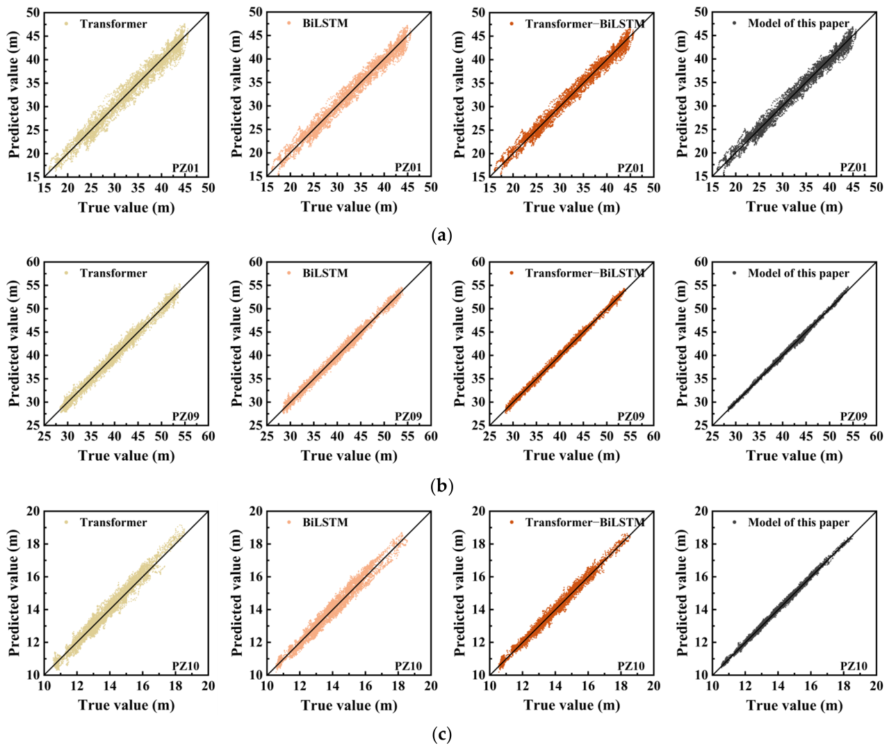
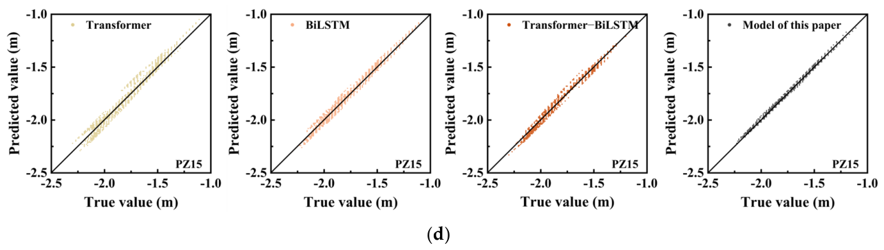
To quantitatively validate the prediction accuracy and global generalization performance of the developed model, scatter plots comparing measured versus predicted values at all monitoring points are presented in Figure 12, and the evaluation metrics and improvement statistics are summarized in

Table 4. Predicted evaluation indicators for measuring points.

PZ01
MODEL	Transformer	BiLSTM	Transformer–BiLSTM	Model of this paper
R2	0.9732	0.9800	0.9859	0.9956
RMSE/m	1.0691	0.9192	0.7192	0.3116
MAE/m	1.0060	0.8730	0.7256	0.6697
MAPE/%	3.1591	2.7869	2.3315	1.8213
PZ09
MODEL	Transformer	BiLSTM	Transformer–BiLSTM	Model of this paper
R2	0.9796	0.9848	0.9863	0.9981
RMSE/m	0.8022	0.5976	0.3966	0.1867
MAE/m	0.6600	0.4770	0.3175	0.2199
MAPE/%	1.6957	1.2108	0.8148	0.5490
PZ10
MODEL	Transformer	BiLSTM	Transformer–BiLSTM	Model of this paper
R2	0.9743	0.9796	0.9869	0.9963
RMSE/m	0.3108	0.2866	0.1880	0.1001
MAE/m	0.2512	0.2345	0.1471	0.0801
MAPE/%	1.8257	1.6832	1.0720	0.5965
PZ15
MODEL	Transformer	BiLSTM	Transformer–BiLSTM	Model of this paper
R2	0.9649	0.9749	0.9850	0.9947
RMSE/m	0.0427	0.0361	0.0279	0.0165
MAE/m	0.0331	0.0301	0.0219	0.0130
MAPE/%	1.9101	1.7370	1.2202	0.7645

Note: The proposed model dynamically selects between ridge regression and Transformer–BiLSTM via the COI.

and

Table 5. Performance improvement results for measurement points.

PZ01				PZ09
Model	Transformer	BiLSTM	Transformer- BiLSTM	Model	Transformer	BiLSTM	Transformer- BiLSTM
R2/%	2.3017	1.5918	0.9839	R2/%	1.8885	1.3505	1.1964
RMSE/%	70.8540	66.1010	56.6741	RMSE/%	76.7265	68.7584	52.9249
MAE/%	33.4294	23.2875	7.7040	MAE/%	66.6818	53.8994	30.7402
MAPE/%	42.3475	34.6478	21.8829	MAPE/%	67.6240	54.6581	32.6215
PZ10				PZ15
Model	Transformer	BiLSTM	Transformer- BiLSTM	Model	Transformer	BiLSTM	Transformer- BiLSTM
R2/%	2.2580	1.7048	0.9525	R2/%	3.0884	2.0310	0.9848
RMSE/%	67.7928	65.0733	46.7553	RMSE/%	61.3583	54.2936	40.8602
MAE/%	68.1131	65.8422	45.5472	MAE/%	60.7251	56.8106	40.6393
MAPE/%	67.3276	64.5615	44.3563	MAPE/%	59.9759	55.9873	37.3463

.

Table 4 and Table 5 show multi-index comparisons of RMSE, MAE and MAPE at four typical seepage pressure points. The proposed model yields markedly lower errors than Transformer, BiLSTM and Transformer BiLSTM benchmarks across all points, with a distinct error reduction advantage. For PZ01 behind the impervious curtain, MAE is only 0.6697m (33.43% lower than the single Transformer model), R² reaches 0.9956, and RMSE drops to 0.3116 m. This demonstrates high-precision fitting for seepage series in regions with high water heads and strong annual periodic fluctuations. For PZ10 in the dam foundation drainage zone, RMSE falls from 0.3108 m (Transformer) to 0.1001 m (67.79% reduction) with R² of 0.9963, confirming accurate capture of seepage variation patterns under elevated high frequency disturbances from drainage regulation. For PZ15, the low-head steady seepage point at the downstream dam toe, the model retains the lowest error level, further verifying its adaptability to zones with distinct fluctuation features. Correlation scatter plots in Figure 12 corroborate these findings, where the diagonal marks the ideal benchmark of perfect prediction measurement agreement. The three benchmarks show highly scattered distributions and notable diagonal deviations, while all sample points of the proposed model closely follow the diagonal without significant systematic bias, indicating smaller overall prediction deviation. Comprehensive results confirm that the model achieves high-quality fitting for both long-term evolution trends and local small-amplitude fluctuations across all locations, including the impervious curtain section, drainage zone and downstream dam toe.

In summary, the proposed model achieves refined seepage pressure prediction across all dam regions via multi-scale preprocessing and differentiated modeling, with outstanding performance, high prediction accuracy and robustness. All monitoring points yield optimal error metrics with R² values exceeding 0.99, demonstrating excellent goodness of fit. It maintains stable high-precision fitting for diverse scenarios, including flat dam bases, periodic fluctuations in the middle and upper dam body, and complex nearshore constraints, breaking through the limitations of traditional models. The core advantage stems from the synergistic design of multi-scale feature decoupling and differentiated modeling, and model selection guided by the COI comprehensive optimization index, which effectively integrates machine learning methods with the physical mechanisms of dam seepage. Noise-assisted EEMD effectively suppresses mode mixing, and IMF component classification aligned with engineering driving mechanisms provides physical inputs for differentiated modeling. The dual-model adaptive system performs parallel training for the component of frequency differentiation to achieve matching precise model components. The COI addresses the one-sidedness of single index evaluation, enabling comprehensive capture and coverage of full-scale seepage pressure features.

5. Discussion

As demonstrated by the foregoing comparative analysis, the multi-scale preprocessing and dual-model fusion framework proposed in this study substantially improve seepage pressure prediction accuracy relative to single-baseline models. More importantly, it systematically addresses the limitations of existing models in terms of physical interpretability from the practical engineering requirements of concrete dam safety monitoring.

Competitive models (Transformer, BiLSTM, Transformer–BiLSTM) exhibit acceptable overall fitting performance, yet their black-box structures cannot distinguish whether seepage pressure anomalies stem from rapid water level variations, periodic temperature fluctuations or time-dependent degradation of the impervious curtain. The concrete dam seepage field results from coupled mechanisms including water level action, rainfall infiltration, thermal stress and long-term aging [39,40]. Modeling raw time series directly mixes multi-scale features. Minor seepage pressure rises induced by local chemical dissolution of the curtain or foundation contact erosion are embedded in intermediate-frequency IMF components. Such weak anomalies are readily masked by annual water level cycles and high frequency noise, triggering false and missed alarms against seepage failure and failing early warning demands. In this study, EEMD adaptively decomposes raw seepage series into multi-scale IMF components with definite physical interpretations. The COI enables dynamic selection between ridge regression and Transformer–BiLSTM, matching each frequency component to an optimal model corresponding to its seepage driving mechanism and facilitating the physical interpretability of predictions. Furthermore, the nonlinear fusion layer replaces traditional linear superposition, preserving implicit cross-scale coupling information and improving reconstruction accuracy.

Benefiting from the independence of each IMF component after EEMD decoupling, the proposed framework supports modular segmentation and hierarchical invocation. For routine inspections that only require the long-term evolutionary trend of the seepage field, the ridge regression module can be activated independently to rapidly output low-frequency time-dependent components. When fine capture of hysteretic seepage responses is necessary, the Transformer–BiLSTM module is employed to fit medium–high frequency components. This hierarchical scheduling strategy allocates computing resources flexibly according to monitoring alert levels and on-site computing capacity, balancing timeliness and computational efficiency, and outperforms the one-size-fits-all deployment of global deep neural networks by a notable margin.

For seepage fields with prominent spatial heterogeneity, globally unified networks suffer weak generalization [41]. Low-frequency long-term seepage evolution is dominated by linear time-variant features with severe multicollinearity among drivers, which triggers overfitting and long-term prediction drift in deep learning. By contrast, medium–high frequency components contain intricate bidirectional nonlinear temporal dependencies and multi-step lag effects that cannot be well captured by linear statistical models. A single network yields acceptable performance only for riverbed zones with uniform water heads behind the impervious curtain, yet produces drastically enlarged errors and scattered precision at measuring points near dam abutments, curtain edges, drainage galleries and dam toes where seepage boundaries and hydraulic gradients change abruptly. The proposed differentiated dual-model framework dynamically assigns the optimal submodel to each IMF via COI combined with nonlinear fusion reconstruction. It resolves the structural conflict that single models fail to simultaneously capture long-term linear trends and nonlinear fluctuations, delivering stable prediction accuracy across all dam measuring points.

In practical dam safety monitoring, warning thresholds for measuring points behind grout curtains are determined by designed uplift pressure and allowable hydraulic gradients. Baseline models yield test-set RMSE ranging from 0.3 to 1.1 m, whose error bands overlap heavily with normal water-level-induced seepage fluctuations, triggering frequent false or missed alarms during flood seasons. The proposed model reduces RMSE to 0.01–0.4 m, narrowing the overall error range below typical warning limits and improving risk identification reliability greatly. For high-risk zones with complex constraints such as dam abutment curtain edges and toe drainage areas, MAPE declines by over 40%. These regions are prone to seepage failure, and the accuracy gain substantially strengthens monitoring performance over hazardous seepage pathways.

The proposed methodology is extendable to various hydraulic structures and complex working conditions. The EEMD-based multi-scale decoupling and COI-guided dual-model optimization framework is not restricted to the seepage pressure forecasting of concrete hyperbolic arch dams. It can also be transferred to nonstationary time-series prediction tasks such as uplift pressure for gravity dams and phreatic line of earth–rock dams, possessing favorable engineering practicability and methodological universality.

6. Conclusions

Accurate seepage pressure prediction is essential for the scientific evaluation of concrete dam service performance. Targeting the strong nonlinearity, nonstationarity and multi-scale coupling of seepage pressure time series, this paper explores the influencing factors in the seepage pressure statistical model of concrete dams, and identifies water level, rainfall, temperature and time as the influencing factors and develops a seepage pressure prediction method integrating EEMD multi-scale preprocessing, ridge regression and Transformer–BiLSTM dual-model fusion. Verified by field monitoring data and comparative experiments on a concrete double-curvature arch dam in Sichuan, China, the model effectiveness is validated, with main conclusions as follows:

(1) EEMD preprocessing provides structured data support for high-precision seepage pressure prediction. It decomposes nonstationary seepage series into IMF components free of prominent mode mixing. Component screening based on seepage physical mechanisms, decoupling high-frequency monitoring noise and instantaneous rainfall disturbances, medium-frequency periodic responses of reservoir level and temperature, and long-term low-frequency seepage field evolution, thus enhancing physical interpretability.

(2) The COI-guided parallel strategy of ridge regression and Transformer–BiLSTM effectively overcomes the structural limitations of single models and the one-sidedness of single index optimization. Ridge regression fits low-frequency linear trend components, while Transformer–BiLSTM adapts to medium-high frequency nonlinear fluctuations.

(3) The proposed fusion model delivers high prediction accuracy and strong spatial adaptability. For typical monitoring points across multiple representative seepage functional zones, the model achieves R² above 0.99 in test set, with RMSE, MAE and MAPE significantly outperforming benchmark models. It exhibits excellent generalization and robustness for seepage pressure series with diverse evolution patterns.

(4) The model has remarkable engineering application value. The framework effectively addresses the accuracy deficiency of traditional seepage safety assessment and early-warning methods, advancing dam seepage safety management from post-event anomaly analysis to pre-event accurate prediction.

(5) Several limitations warrant note. First, training data cover mainly normal hydrological events, leaving the model’s reliability under extreme situations unverified, as seepage mechanisms may then shift beyond the training distribution. Second, geological complexity is presently treated only via implicit time-dependent corrections. Future work should explicitly weight geological features (lithology, geotechnical parameters, fracture distribution, schistosity, chemical bandation, and weathering susceptibility) as covariates to enhance physical interpretability across heterogeneous foundations. Finally, single-case validation limits generalizability to other dam types or high altitude freeze–thaw environments. Future research should integrate physics-informed constraints, conduct multi-case validation to establish generalized calibration protocols.

References

1. Chen, H.; Huang, S.; Xu, Y.-P.; Teegavarapu, R.S.V.; Guo, Y.; Nie, H.; Xie, H. Using baseflow ensembles for hydrologic hysteresis characterization in humid basins of Southeastern China. Water Resour. Res. 2024, 60, e2023WR036195. [Google Scholar] [CrossRef] [Scilit]
2. Liu, G.; Zhou, Z.; Xu, S.; Mi, W. Hysteresis of dam slope safety factor under water level fluctuations based on the LEM coupled with FEM Method. CMES-Comp. Model. Eng. 2022, 133, 351–375. [Google Scholar] [CrossRef] [Scilit]
3. Hua, G.W.; Wang, S.J.; Xiao, M.; Hu, S.H. Research on the Uplift Pressure Prediction of Concrete Dams Based on the CNN-GRU Model. Water 2023, 15, 319. [Google Scholar] [CrossRef] [Scilit]
4. Su, Z.; Chen, G.; Meng, Y. Study on seepage characteristics and stability of core dam under the combined action of the variation of reservoir water level and rainfall. Geotech. Geol. Eng. 2021, 39, 193–211. [Google Scholar] [CrossRef] [Scilit]
5. Qian, R.; Zhu, Y.; Duan, Y.; Xu, W.; Song, Z.; Zhang, P.; Niu, X. Mechanical properties and damage model of basalt fiber reinforced concrete under sulfate attack. J. Build. Eng. 2026, 124, 115968. [Google Scholar] [CrossRef] [Scilit]
6. Zhu, Y.; He, W.; Niu, X.; Lu, J.; Xiang, Y.; Wang, Y. Efficient remotely operated vehicle-based deep learning framework for detecting underwater blockages in hydropower infrastructure. Autom. Constr. 2026, 190, 107124. [Google Scholar] [CrossRef] [Scilit]
7. Salazar, F.; Morán, R.; Toledo, M.Á.; Oñate, E. Data-based models for the prediction of dam behaviour: A review and some methodological considerations. Arch. Comput. Methods Eng. 2017, 24, 1–21. [Google Scholar] [CrossRef] [Scilit]
8. Li, B.; Yang, J.; Hu, D. Dam monitoring data analysis methods: A literature review. Struct. Control Health Monit. 2020, 27, e2501. [Google Scholar] [CrossRef] [Scilit]
9. Zhang, H.; Li, Z.; Li, W.; Song, Z.; Ge, W.; Han, R.; Wang, T. Risk Analysis of instability failure of earth–rock dams based on the fuzzy set theory. Water 2021, 13, 3088. [Google Scholar] [CrossRef] [Scilit]
10. Wang, L.; Mao, Y.; Cheng, Y.; Liu, Y. Deep learning-based diagnosing structural behavior in dam safety monitoring system. Sensors 2021, 21, 1171. [Google Scholar] [CrossRef] [Scilit] [PubMed]
11. Song, J.; Liu, Y.; Yang, J. Dam safety evaluation method after extreme load condition based on health monitoring and deep learning. Sensors 2023, 23, 4480. [Google Scholar] [CrossRef] [Scilit] [PubMed]
12. Rehamnia, I.; Al-Janabi, A.M.S.; Sammen, S.S.; Pham, B.T.; Prakash, I. Prediction of seepage flow through earthfill dams using machine learning models. HydroResearch 2024, 7, 131–139. [Google Scholar] [CrossRef] [Scilit]
13. Dai, Q.W.; Zhou, W.; He, R.; Yang, J.S.; Zhang, B.; Lei, Y. A Data Assimilation Methodology to Analyze the Unsaturated Seepage of an Earth-Rockfill Dam Using Physics-Informed Neural Networks Based on Hybrid Constraints. Water 2024, 16, 1041. [Google Scholar] [CrossRef] [Scilit]
14. Prakash, G.; Dugalam, R.; Barbosh, M.; Sadhu, A. Recent advancement of concrete dam health monitoring technology: A systematic literature review. Structures 2022, 44, 766–784. [Google Scholar] [CrossRef] [Scilit]
15. Cho, M.; Kim, C.; Jung, K.; Jung, H. Water Level Prediction Model Applying a Long Short-Term Memory (LSTM)–Gated Recurrent Unit (GRU) Method for Flood Prediction. Water 2022, 14, 2221. [Google Scholar] [CrossRef] [Scilit]
16. Yang, B.; Xiao, T.; Wang, L.; Huang, W. Using Complementary Ensemble Empirical Mode Decomposition and Gated Recurrent Unit to Predict Landslide Displacements in Dam Reservoir. Sensors 2022, 22, 1320. [Google Scholar] [CrossRef] [Scilit] [PubMed]
17. Xie, J.; Shao, Y.; Li, J.; Jia, Z.; Fu, C.; Shao, C.; Xu, Y.; Hu, Y. Explainable Monitoring Model Based on AE-BiGRU and SHAP Analysis of Seepage Pressure for Concrete Dams. Water 2026, 18, 614. [Google Scholar] [CrossRef] [Scilit]
18. Chen, H.; Wang, K.; Zhao, M.; Chen, Y.; He, Y. A CNN-LSTM-attention based seepage pressure prediction method for Earth and rock dams. Sci. Rep. 2025, 15, 12960. [Google Scholar] [CrossRef] [Scilit] [PubMed]
19. Zhu, Y.; Zhang, Z.; Gu, C.; Li, Y.; Zhang, K.; Xie, M. A coupled model for dam foundation seepage behavior monitoring and forecasting based on variational mode decomposition and improved temporal convolutional network. Struct. Control Health Monit. 2023, 2023, 3879096. [Google Scholar] [CrossRef] [Scilit]
20. Li, F.; Ma, G.; Chen, S.; Huang, W. An ensemble modeling approach to forecast daily reservoir inflow using bidirectional long-and short-term memory (Bi-LSTM), variational mode decomposition (VMD), and energy entropy method. Water Resour. Manag. 2021, 35, 2941–2963. [Google Scholar] [CrossRef] [Scilit]
21. Rezaie-Balf, M.; Naganna, S.R.; Kisi, O.; El-Shafie, A. Enhancing streamflow forecasting using the augmenting ensemble procedure coupled machine learning models: Case study of Aswan High Dam. Hydrol. Sci. J. 2019, 64, 1629–1646. [Google Scholar] [CrossRef] [Scilit]
22. Fatehi-Nobarian, B.; Fard Moradinia, S. Wavelet–ANN hybrid model evaluation in seepage prediction in nonhomogeneous earthen dams. Water Pract. Technol. 2024, 19, 2492–2511. [Google Scholar] [CrossRef] [Scilit]
23. Wei, B.; Luo, S.; Xu, F.; Yuan, D.; Zhang, W. Combined Model for Displacement Prediction of Concrete Arch Dam Based on Monitoring Time Series Decomposition and Reconstruction. Eng. Sci. Technol. 2022, 54, 51–63. [Google Scholar] [CrossRef]
24. Wang, M.; Wang, H.; Zhang, F. DTSformer: A Dual-Branch Transformer with Multi-scale Decomposition for Long-Term Time Series Forecasting. Mach. Learn. 2026, 115, 105. [Google Scholar] [CrossRef] [Scilit]
25. Kong, H.; Ding, Y.; Li, D. A Dam Deformation Prediction Model Coupled with Secondary Mode Decomposition and Optimized LightGBM. Geod. Geodyn. 2025, 45, 1171–1179. [Google Scholar] [CrossRef]
26. Li, Y.; Sun, X.; Li, G.; Zhang, J.; Fang, D.; Wang, X. Impact of concrete face cracks on the saturated and unsaturated seepage behavior of rockfill dams. Structures 2024, 61, 105990. [Google Scholar] [CrossRef] [Scilit]
27. Zhang, X.; Chen, X.D.; Li, J.J. Improving Dam Seepage Prediction Using Back-Propagation Neural Network and Genetic Algorithm. Math. Probl. Eng. 2020, 2020, 1404295. [Google Scholar] [CrossRef] [Scilit]
28. Fu, C.; Wang, Q.; Shao, C.; Xu, Y.; Zheng, S. Analysis of Embankment Seepage Responses Based on Physics-Informed Neural Networks Surrogate Model. Water 2026, 18, 749. [Google Scholar] [CrossRef] [Scilit]
29. Li, D.Q.; Kang, Q.; Wang, R.H.; He, J.P.; Liu, Y. Application of artificial intelligence models in the seepage flow prediction of dam: A case study of Shenzhen reservoir. Georisk Assess. Manag. Risk Eng. Syst. Geohazards 2025, 19, 944–965. [Google Scholar] [CrossRef] [Scilit]
30. Shu, Y.K.; Shen, Z.Z.; Xu, L.Q.; Duan, J.R.; Ju, L.Y.; Liu, Q. Inverse Modeling of Seepage Parameters Based on an Improved Gray Wolf Optimizer. Appl. Sci. 2022, 12, 8519. [Google Scholar] [CrossRef] [Scilit]
31. Lu, Y.; Huang, M.; Lan, Z. Application of artificial neural network model on back analysis of permeability parameters for unsteady seepage of seawall. South-North Water Transf. Water Sci. Technol. 2015, 13, 1147–1150. [Google Scholar]
32. Wu, Z.; Huang, N.E. Ensemble empirical mode decomposition: A noise-assisted data analysis method. Adv. Adapt. Data Anal. 2009, 1, 1–41. [Google Scholar] [CrossRef] [Scilit]
33. Vaswani, A.; Shazeer, N.; Parmar, N.; Uszkoreit, J.; Jones, L.; Gomez, A.N.; Kaiser, Ł.; Polosukhin, I. Attention is all you need. In Proceedings of the 31st International Conference on Neural Information Processing Systems, Long Beach, CA, USA, 4–9 December 2017; pp. 6000–6010. [Google Scholar]
34. Graves, A.; Fernández, S.; Schmidhuber, J. Bidirectional LSTM networks for improved phoneme classification and recognition. In Proceedings of the International Conference on Artificial Neural Networks, Warsaw, Poland, 11–15 September 2005; pp. 799–804. [Google Scholar]
35. Nassiri, K.; Akhloufi, M. Transformer models used for text-based question answering systems. Appl. Intell. 2023, 53, 10602–10635. [Google Scholar] [CrossRef] [Scilit]
36. Mayer, C.W.; Ludwig, S.; Brandt, S. Prompt text classifications with transformer models! An exemplary introduction to prompt-based learning with large language models. J. Res. Technol. Educ. 2023, 55, 125–141. [Google Scholar] [CrossRef] [Scilit]
37. Liu, L.; Jin, Y.; Zhang, S.; Cheng, F. Dam Seepage Analysis Based on Causal Testing and Regression Analysis. Water 2026, 18, 1359. [Google Scholar] [CrossRef] [Scilit]
38. Yang, X.; Xiang, Y.; Wang, Y.; Shen, G. A dam safety state prediction and analysis method based on EMD-SSA-LSTM. Water 2024, 16, 395. [Google Scholar] [CrossRef] [Scilit]
39. Qiu, H.; Zhu, S.; Fang, H.; Lu, X. Study of Seepage Laws of Deep Rock Mass Under Different Water Temperatures Based on Porous Media. Water 2025, 17, 357. [Google Scholar] [CrossRef] [Scilit]
40. Zhang, D.; Liu, Y.; Jiang, Y.; Luo, Y. Study on the Allowable Gradient of Soil at the Base of a Cutoff Wall Considering Stress State. Water 2026, 18, 1420. [Google Scholar] [CrossRef] [Scilit]
41. Alrowais, R.; Alwushayh, B.; Bashir, M.T.; Nasef, B.M.; Ghazy, A.; Elkamhawy, E. Modeling and analysis of cutoff wall performance beneath water structures by feed-forward neural network (FFNN). Water 2023, 15, 3870. [Google Scholar] [CrossRef] [Scilit]
Figure 1. Flowchart of the EEMD method.
Water 18 02049 g001
Figure 2. Geometric schematic of ridge regression.
Water 18 02049 g002
Figure 3. Basic structure diagram of Transformer.
Water 18 02049 g003
Figure 4. Basic structure diagram of BiLSTM.
Water 18 02049 g004
Figure 5. The overall architecture of this model.
Water 18 02049 g005
Figure 6. The implementation process of this model.
Water 18 02049 g006
Figure 7. Seepage pressure monitoring layout of the double-curvature arch dam.
Water 18 02049 g007
Figure 8. Actual measurement curves of water level and rainfall volume.
Water 18 02049 g008
Figure 9. EEMD of the data images. (a) PZ01; (b) PZ09; (c) PZ10; (d) PZ15.
Water 18 02049 g009
Figure 10. The loss of IMFs over the course of iterations.
Water 18 02049 g010
Figure 11. Comparison chart of predicted values and actual values for different models. (a) PZ01; (b) PZ09; (c) PZ10; (d) PZ15.
Water 18 02049 g011aWater 18 02049 g011b
Figure 12. Correlation scatter plots for monitoring points. (a) PZ01; (b) PZ09; (c) PZ10; (d) PZ15.
Water 18 02049 g012aWater 18 02049 g012b