Dynamics of the Turbidity Maximum Zone and Its Relationship with the Salt-Wedge Position in a High-Discharge Microtidal Estuary

Abstract

The Magdalena River Estuary hosts the access channel to the Port of Barranquilla, where recurrent dredging is required to maintain navigable depths of up to approximately 12 m. Chronic siltation in this channel is closely linked to the dynamics of the Turbidity Maximum Zone (TMZ), which remain poorly understood in tropical, microtidal systems with extreme sediment loads. This study investigates the spatiotemporal variability of the TMZ in the Magdalena River Estuary (MRE), Colombia, using a previously calibrated and validated MOHID 3D numerical model coupled with sediment transport. Sixteen scenarios covering river discharges from 2000 to 5500 m³ s⁻¹ under neap and spring tidal conditions were analyzed. Results show that the TMZ core position follows a nonlinear inverse relationship with discharge (R² = 0.976), migrating from km 13–15 under extreme low-flow conditions (Q = 2000 m³ s⁻¹) to the estuary mouth for discharges above 5000 m³ s⁻¹. Within the simulated discharge range of 2000–5500 m³ s⁻¹ and under the modeled neap and spring tidal conditions, the position where ε = 0.005 tracks the TMZ core location (R² = 0.96, RMSE ≈ 1 km), suggesting that this threshold can be used as a first-order spatial indicator of maximum sedimentation under the conditions evaluated in this study. Contrary to macrotidal estuaries, the MRE exhibits higher suspended-sediment concentrations during neap tides than during spring tides, with SSC up to 77 percent greater for Q = 2000 m³ s⁻¹. This reversal is driven by the suppression of turbulent mixing (R_i > 20) during neap conditions, which preserves the salt-wedge structure and enhances stratification-controlled sediment trapping. These results provide two process-based criteria for predicting turbidity-maximum behavior in the MRE: the ε = 0.005 stratification isoline and the discharge–TMZ polynomial. More broadly, the methodological framework may support the development of site-specific predictors for other highly stratified, microtidal estuaries subject to strong discharge variability.

1. Introduction

Estuaries, where seawater mixes with continental freshwater [1], are characterized by pronounced longitudinal density gradients [2,3] and are commonly classified by their degree of stratification as well-mixed, partially mixed, or highly stratified systems [4,5]. In highly stratified, microtidal systems, the suppression of vertical mixing by buoyancy forces leads to the formation of a salt wedge that intrudes along the channel bed [6,7], creating conditions that govern sediment trapping and the formation of the turbidity maximum zone (TMZ). In this sense, estuaries function as transition zones where oceanic and fluvial processes interact. This transition generates spatial gradients in multiple environmental conditions throughout the estuary; for example, salinity ranges from typical seawater values to freshwater, and variations are also observed in sediment grain size, biodiversity, water-column turbidity, and chemical composition as conditions shift from riverine to marine [8,9,10,11]. For these reasons, estuaries are highly complex and ecologically valuable ecosystems, yet they are also particularly vulnerable to the impacts of climate change and the intensification of extreme events [12,13,14].

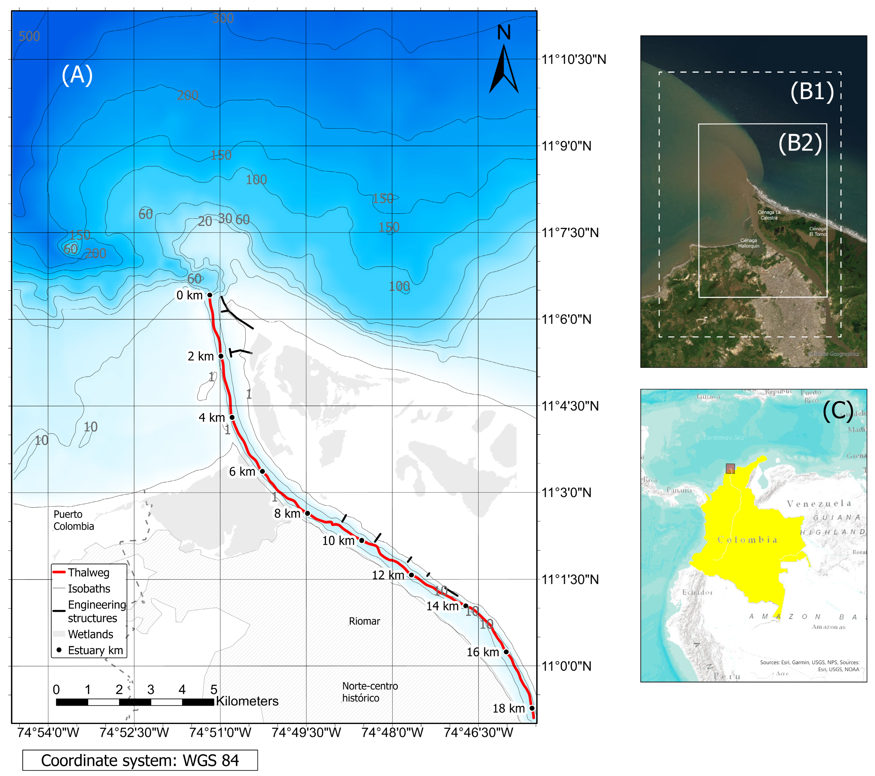
In the Colombian Caribbean, the Magdalena River delta forms a highly stratified estuary under low-discharge conditions. This estuary is characterized as wave-dominated and exhibits exceptionally high river and sediment discharge [12,13] (Figure 1). Variations in freshwater discharge influence salinity distribution and the patterns of gravitational circulation, thereby affecting sediment transport, deposition, and resuspension [14].

Sediment dynamics in estuaries give rise to the formation of the turbidity maximum zone (TMZ), which corresponds to a region where suspended-sediment concentrations are significantly higher than in the rest of the estuary [15,16,17]. The turbidity maximum develops as a result of estuarine circulation patterns, which are convergent in the lower part of the water column. The efficiency of sediment trapping depends on the settling velocity and the strength of estuarine circulation [18]. The formation of the TMZ is driven by sediment trapping and flocculation, processes controlled by the advection of water masses with different densities and by turbulence [6,14]. Tidal asymmetry induces landward transport of suspended sediments, generating an additional sediment trap [19]. In some cases, the development of the TMZ is associated with bathymetric features, forming in areas with depth transitions where reduced flow velocity promotes the convergence of suspended particulate material [20]. Overall, the formation of the TMZ is a dynamic process regulated by gravitational and residual circulation, mixing conditions, and sediment properties [14,21].

The formation and position of the TMZ are governed by the interplay of three main mechanisms, namely gravitational circulation, stratification-induced suppression of turbulence, and tidal asymmetry [6,18,20]. River discharge exerts a first-order control on TMZ location by modulating the extent of saline intrusion and, consequently, the position of the convergence front where sediment trapping occurs. In the Loire River estuary (France), ref. [22] showed that the TMZ migrates landward during low-flow periods (300–360 m³ s⁻¹), whereas its downstream retreat requires substantially higher discharges (467–1034 m³ s⁻¹); they attributed this hysteresis to the formation of a mobile mud layer that resists remobilization. Similarly, in the Changjiang Estuary (China), ref. [23] used 30 years of satellite data to demonstrate that the TMZ is primarily controlled by sediment supply, which is itself a function of river discharge. Ref. [24] confirmed the strong influence of discharge variability on TMZ behavior in the Yellow River estuary through four decades of Landsat imagery, also highlighting the role of estuarine morphology and wind forcing. Stratification plays a complementary role by controlling the vertical distribution of suspended sediments and the efficiency of turbulent mixing. In the Changjiang Estuary, ref. [16] found that the vertical SSC structure is mainly governed by stratification resulting from the interaction between river discharge and saline intrusion. Ref. [6] demonstrated that the suppression of turbulence by salt stratification greatly enhances sediment trapping near the landward limit of salinity intrusion, a process that can be several times more effective than gravitational convergence alone for silt-sized particles. Additionally, tidal asymmetry induces a net landward transport of suspended sediments that reinforces the sediment trap [19]. In macrotidal systems, tidal pumping has been shown to be a dominant mechanism for TMZ formation [15], while in partially mixed estuaries, ref. [25] demonstrated that the modulation of stratification by tidal straining controls sediment retention through asymmetric pumping.

Studies on the TMZ have focused predominantly on mesotidal and macrotidal estuaries at mid-latitudes (e.g., Gironde, Thames, Ems), where cyclical resuspension dominates sediment dynamics [19,26]. In contrast, tropical high-discharge systems exhibit fundamentally different behavior. In these environments, tidal kinetic energy is often insufficient to overcome the stratification imposed by river discharge, resulting in systems where the position of the TMZ is controlled almost exclusively by the physics of the salt-wedge front and the suppression of turbulence at the pycnocline [6,27]. The Magdalena River, with a sediment discharge of 144 × 10⁶ tons per year [28], represents an extreme case of this regime, where the influence of stratification on sediment transport is particularly pronounced.

However, to our knowledge, no previous study has systematically quantified a stratification threshold that predicts TMZ-core position across a wide range of discharge scenarios in a tropical, microtidal, highly stratified estuary with extreme sediment loads. Moreover, while macrotidal estuaries typically exhibit higher suspended-sediment concentrations during spring tides due to enhanced tidal resuspension [15,19], it remains unclear whether this pattern holds in microtidal systems where tidal energy is insufficient to dominate over stratification-induced trapping. Addressing these gaps is essential for understanding sediment dynamics in river-dominated estuaries and for developing predictive tools for sedimentation management.

In the Magdalena River Estuary (MRE), the spatial variability of the TMZ depends on the position of the freshwater–saltwater interface (FSI), defined as the location where the 1-psu isohaline intersects the riverbed, since the core of the TMZ typically forms near the FSI and is always located downstream from it [14]. Along the contact surface between riverine and oceanic waters, flow velocity approaches zero due to the convergence of the two water masses [29]. Flocculation is one of the main mechanisms contributing to the formation of the TMZ because, as water-column stratification becomes more stable, the efficiency of bottom-generated turbulence to mix the water column decreases. This reduction in mixing limits the capacity to keep sediments in suspension, thereby promoting their settling and the formation of flocs [14].

Understanding sediment dynamics in the MRE is essential because the Port of Barranquilla is located within this area and experiences chronic sedimentation along the navigation channel. The access channel to the Port of Barranquilla requires frequent maintenance dredging due to recurrent sedimentation. Technical specifications indicate design dredging depths of approximately 11.4–12.2 m along the channel and identify the most critical sedimentation/intervention areas near the river mouth [30]. More recently, Cormagdalena’s institutional analytics platform reported 52 dredging events in Barranquilla and a total dredged volume of approximately 3.84 × 10⁶ m³ for 2025. These figures highlight the operational importance of understanding the mechanisms controlling sediment trapping, TMZ migration, and high-SSC zones in the Magdalena River Estuary [31].

Over the last century, several engineering interventions have been implemented to improve navigability, altering sediment distribution and, consequently, the morphology of the channel [32]. Since 1936, the estuary has been constrained to a single outlet channel by two jetties, which were reinforced and extended between 1949 and 1951. Later, between 1994 and 1995, a retaining wall and contraction dikes were constructed to close a secondary channel, and between 2008 and 2009 two additional contraction dikes were built on the eastern jetty [33]. For these reasons, understanding sediment behavior in the MRE could support the development of more sustainable and long-lasting strategies to maintain navigability along the channel while minimizing impacts on adjacent ecosystems, as well as improving the planning of dredging operations. This is feasible when the locations where sedimentation is likely to concentrate throughout the MRE can be identified as a function of river discharge.

In this context, the present study aims to analyze the dynamics of the TMZ, that is, the variations in its position and suspended-sediment concentration under different river-discharge and tidal scenarios in the MRE, a high-discharge microtidal system. Additionally, we seek to establish the relationship between the positions of the FSI and the TMZ in order to develop improved predictive schemes for identifying areas within the MRE where sedimentation processes are expected to intensify, thereby enabling better management of dredging activities along the navigation channel. To achieve this, we analyze the Magdalena River discharge time series and perform numerical simulations using a calibrated three-dimensional model for the study area. Subsequently, we compute the stratification parameter (ε), the bulk Richardson number (R_i), and the turbulent kinetic energy production (P), following the methodology described by [29,34,35]. Finally, the position of the TMZ is determined from the outputs of the numerical simulations.

Unlike previous MOHID applications in the Magdalena River Estuary, which focused on the seasonal variability of stratification and mixing [29], salt-wedge intrusion [34], or wave effects on estuarine hydrodynamics [35], the present study directly examines the dynamics of the turbidity maximum. It derives a stratification-based predictor of TMZ-core position using the ε = 0.005 isoline, establishes a quantitative discharge–TMZ relationship, identifies a neap–spring reversal in suspended-sediment concentration, and demonstrates the spatially variable contribution of suspended sediment to the estuarine density structure.

2. Study Area

The MRE is located in the Colombian Caribbean, a region that exhibits two main seasons throughout the year due to the migration of the Intertropical Convergence Zone (ITCZ). The dry season extends from December to May, while the wet season dominates the remaining months, interrupted by the Veranillo de San Juan between June and July, a relatively dry period [36]. At longer timescales, variations in hydrological patterns are driven by the prevailing phase of the El Niño–Southern Oscillation (ENSO) [29]. During El Niño (warm phase), precipitation and river discharge decrease, in contrast to La Niña (cold phase), when both increase [37]. In the dry season, the mean significant wave height (Hs) in the Colombian Caribbean is 1.42 m, whereas during the wet season it decreases to 0.9 m, with waves predominantly arriving from the NE [38]. Surface salinity ranges between 33 and 37 on the Practical Salinity Scale [32]. The Colombian Caribbean exhibits a microtidal regime, with tidal ranges between 0.13 and 0.40 m, and a mixed tide predominantly diurnal in the Magdalena delta [39].

The mouth of the MRE is approximately 540 m wide and has a minimum depth of 9.5 m [29]. The strongest winds occur between December and April, with magnitudes ranging from 7.3 to 9.2 m s⁻¹, whereas during the rest of the year winds are weaker, with an average magnitude of 6.5 m s⁻¹ and prevailing directions from the NE (43%) and NNE (30%) [32]. The Magdalena River is the main sediment source to the Caribbean Sea, delivering approximately 144 × 10⁶ tons per year [28]. Due to the large sediment load, the MRE is classified as turbid (4000 mg L⁻¹ < SSC_max < 10,000 mg L⁻¹) and extremely turbid (SSC_max > 10,000 mg L⁻¹) during low-flow conditions [14]. River discharge varies seasonally, reaching about 9000 m³ s⁻¹ during the wet season and 4000 m³ s⁻¹ in the dry season [33].

In the MRE, [29] found that the maximum penetration of the salt wedge is 21 km and occurs during the warm ENSO phase in the dry season (Q = 2000 m³ s⁻¹). Under neutral ENSO conditions during the same season (Q = 3800 m³ s⁻¹), saline intrusion extends only up to 6 km, whereas during the cold ENSO phase in the dry season and during any ENSO phase in the wet season, saline intrusion is practically absent. Thus, the length of salt-wedge penetration is directly controlled by river discharge [34]. Ref. [40] reported that the salt wedge in the Magdalena River Estuary is more responsive to changes in discharge than in other highly stratified estuaries due to the forced reduction in channel width implemented to maintain navigability. For discharges above 5200 m³ s⁻¹, the convergence front is located at the mouth, and at this point, freshwater flow detaches from the bed and limits the plume to the surface layer, generating a lift-off regime. They also found that bathymetric features create barriers that influence salt-wedge propagation near km 15 and km 20 [40].

The predominant grain size on the bed is silty very fine sand with a median diameter d₅₀ = 70.6 μm [14]. Approximately 85 percent of the sediment in the MRE is transported in suspension [13]. Of the suspended load, 84.3 percent corresponds to silt-sized particles, while the remaining 15.7 percent corresponds to very fine sand (97.8 percent) and fine sand (2.2 percent). The silt fraction dominates at the surface and in the mid–water column, whereas the sand fraction is more abundant near the bed [41].

Ref. [14] defined the TMZ in the MRE as the region where suspended-sediment concentrations exceed 4500 mg L⁻¹, based on field measurements conducted under a discharge of approximately 4500 m³ s⁻¹, and identified the TMZ core as the area where the highest SSC values are reached. Other approaches in the literature define the TMZ position based on the location of peak SSC along the estuary, either from depth-averaged or near-bed concentrations, without relying on absolute thresholds [18,20,21,42]. In the MRE, ref. [14] found that during the wet season, SSC in the upper part of the water column within the channel ranged between 2200 and 2700 mg L⁻¹, increasing to values above 3500 mg L⁻¹ toward the bottom. During the dry season, SSC reached 3100 mg L⁻¹ in the upper water column and increased to more than 6700 mg L⁻¹ near the bed. Within the TMZ, locally elevated SSC values appear below mid-depth.

Regarding seasonal variability, ref. [15] reported that during the wet-season surveys of 29 and 30 November 2012, the TMZ occupied the reach between km 0.05 and km 4.59 and between km 0.14 and km 1.04 from the river mouth, respectively. The TMZ core was located at km 0.44 on 29 November and at km 0.39 on 30 November. During the dry-season surveys of 20 and 21 April 2013, the TMZ extended farther upstream, occupying the reach between km 1.81 and beyond km 7 and between km 4.62 and beyond km 7 from the river mouth, respectively. The TMZ core was located at km 4.3 on 20 April and at km 6.22 on 21 April.

3. Materials and Methods

3.1. Model Configuration

The simulations were performed using the 2016 version of the MOHID 3D modeling system, following a configuration previously applied and calibrated for the MRE [13,29,32,35].

Across these studies, the model has been validated against field measurements of the variables most relevant to the present analysis, including water level, currents, and salinity [32], the potential energy anomaly, layer Richardson number, and buoyancy frequency that characterize stratification and mixing [29], and suspended-sediment concentration and near-bed shear stress [13]. The salt-wedge intrusion length has likewise been reproduced across 26 discharge–tide scenarios using the same 80 m horizontal resolution and the same Cartesian vertical discretization [34]. The horizontal resolution (Δx = Δy = 80 m) and vertical resolution (47 layers) adopted in the present work are finer than those used in comparable three-dimensional studies of estuarine turbidity maxima and sediment transport, which typically employ 15 to 18 vertical layers and horizontal grid sizes on the order of 100 m [42,43].

MOHID 3D solves the three-dimensional equations for incompressible flows using the Boussinesq and Reynolds approximations and assuming hydrostatic equilibrium [44]. The model employs a finite-volume approach on an Arakawa-C grid for spatial discretization [45]. An alternating-direction implicit (ADI) algorithm is used to solve the equations, computing changes in water level and velocity [46,47]. Salinity and temperature are transported using the momentum equations. The model is well suited for simulating estuarine and coastal flows with strong three-dimensional effects [44]. For vertical turbulence, the General Ocean Turbulence Model (GOTM) is applied [48], while horizontal turbulence is represented through the Smagorinsky scheme [49] with a coefficient of 0.1, as this value yielded the best agreement between modeled and observed data.

Table 1. Previously reported validation metrics for the MOHID 3D model of the Magdalena River Estuary [29,32].

Variable	Bias	RMSE	Willmott	Skill	Campaign	Source
Panel A. Stratification and Mixing Parameters
Potential energy anomaly, φ (J m−3)	−0.018	4.5	0.99	—	2013 (dry)	[29]
Potential energy anomaly, φ (J m−3)	−0.05	6.2	0.99	—	2014 (dry)
Layer Richardson number, Rl	0.06	0.38	0.98	—	2013 (dry)
Layer Richardson number, Rl	−0.08	0.13	0.99	—	2014 (dry)
Buoyancy frequency, β (s−2)	−0.12	0.0010	0.97	—	2013 (dry)
Buoyancy frequency, β (s−2)	−0.0477	0.00014	0.99	—	2014 (dry)
Panel B. Hydrodynamic Variables
Water level (m)	—	0.04	—	0.95	March 2014	[32]
Salinity (Practical Salinity Scale)	—	1.60–2.51	—	0.92–0.96	2012–2013
Velocity (m s−1)	—	0.01–0.08	—	0.80–0.95	2012–2013

Note: The symbol “—” indicates that the corresponding metric was not reported in the original study.

summarizes previously reported calibration and validation metrics from MOHID 3D applications in the MRE using the same hydrodynamic parameterization adopted in the present study [29,32]. The reported metrics include bias, root mean square error (RMSE), the Willmott index of agreement, and the skill score. These metrics are defined as follows. Bias measures the mean systematic error between modeled and observed values, with values close to zero indicating no systematic offset. RMSE quantifies the average magnitude of the error in the same units as the evaluated variable. The Willmott index of agreement ranges from 0, indicating no agreement, to 1, indicating perfect agreement. The skill score compares the model error against the observed variance, with higher values indicating better model performance. Values above 0.5 are generally considered indicative of skillful predictions in coastal–ocean applications [50,51].

For the numerical simulations, an outer grid covering an area of 844 km² was used, consisting of 220 × 150 nodes (Δx = Δy = 160 m and Δt = 8 s) in barotropic mode, with a single vertical layer. This grid was nested with an inner grid (high-resolution grid) covering an area of 387 km², composed of 288 × 212 nodes (Δx = Δy = 80 m and Δt = 4 s), which was run in baroclinic mode and discretized into 47 vertical layers (Figure 1).

The bathymetric information used to construct the computational grids was obtained from the GEBCO global bathymetric database, official local nautical charts, and detailed bathymetric data for the inner estuary. For the inner estuary, a detailed 2018 multibeam bathymetric survey with 1 m resolution was used. The bathymetry was referenced to mean spring low water (MSLW).

The vertical discretization into 47 Cartesian layers was selected to capture the pronounced vertical density gradients characteristic of this salt-wedge system. Over a maximum water depth of about 20 m, this corresponds to an effective layer thickness of approximately 0.4 m, resolving the 1–2 m pycnocline with three to five layers; the Cartesian (Z-level) discretization, unlike terrain-following (sigma) coordinates, further minimizes the artificial diapycnal mixing of scalar properties across the pycnocline [44]. This high vertical resolution is essential for accurately computing the Richardson number (Ri) and turbulence production (P) at the interface, preventing artificial numerical diffusion that could otherwise smooth the stratification. The contrast between the horizontal resolution of 80 m and the vertical resolution of 47 layers reflects the physical scales of the processes represented in the model. The channel width at the mouth is approximately 540 m, while the salt-wedge length varies from about 1 km under high-discharge conditions to approximately 21 km under extreme low-discharge conditions. Therefore, the 80 m horizontal grid resolves these characteristic length scales with approximately 6 to 260 nodes. Horizontal advection terms are not lost, because the salt-wedge front migrates over distances of several kilometres, which are well above the 80 m grid resolution. In addition, cross-channel flow is constrained by the engineered jetties, so the dominant advective gradients are longitudinal and adequately resolved.

The sediment-transport configuration implemented in the model follows the approach proposed by [13]. For sediment-transport calculations, MOHID solves the advection–diffusion equation, in which changes in settling velocity are incorporated into the vertical advection component [13]. MOHID assumes that cohesive sediments are transported exclusively in suspension, an assumption suitable for the MRE since approximately 85 percent of the sediment load is suspended and consists mainly of silts and clays [13]. Accordingly, the measured silt-dominated suspended load, including the minor very fine and fine sand fraction, was represented as a single bulk suspended-sediment class, whose settling behavior is parameterized through the concentration-dependent closure in Equations (1) and (2), rather than through separate grain-size classes. The settling velocity was computed using the equations proposed by [52].

$$Ws=K_1{C}^m\hspace{1em}\hspace{1em}for C<C_{Hs}$$

(1)

$$Ws=K_1\times C_{\left(Hs\right)}^m{\left(1-K_2\left(C-C_{Hs}\right)\right)}^{m1}\hspace{1em}\hspace{1em}for C>C_{Hs}$$

(2)

Ref. [13] established that K₁ = 0.006 m⁴ kg⁻¹ s⁻¹, K₂ = 0.01 m³ kg⁻¹, m = 1, and m₁ = 4.65. These parameters depend on sediment type and salinity. ${\mathrm{C}}_{\mathrm{H}\mathrm{s}}$ corresponds to the concentration above which settling velocity is affected by flocculation and hindered settling, and it is set to 4 kg m⁻³. Ref. [13] also coupled the MOHID 3D hydrodynamic model with the SWAN (Simulating WAves Nearshore) wave model to evaluate the effect of waves, tides, and river discharge on the spatial and temporal dynamics of sediment transport in the MRE.

The calibration was based on a comparison between modeled data and field measurements collected under low-discharge conditions (February–March 2018) and high-discharge conditions (November 2017). The model’s ability to reproduce the spatial and vertical distribution of suspended-sediment concentration (SSC) was evaluated, as well as the sediment-transport patterns influenced by waves, tides, and river discharge. Validation metrics such as the skill score and the Willmott score were used, both exceeding values of 0.5, indicating an adequate representation of SSC behavior in the study area. The calibration results showed that the model successfully reproduced the temporal and spatial variations in SSC and near-bed shear stress (NBSS) [13].

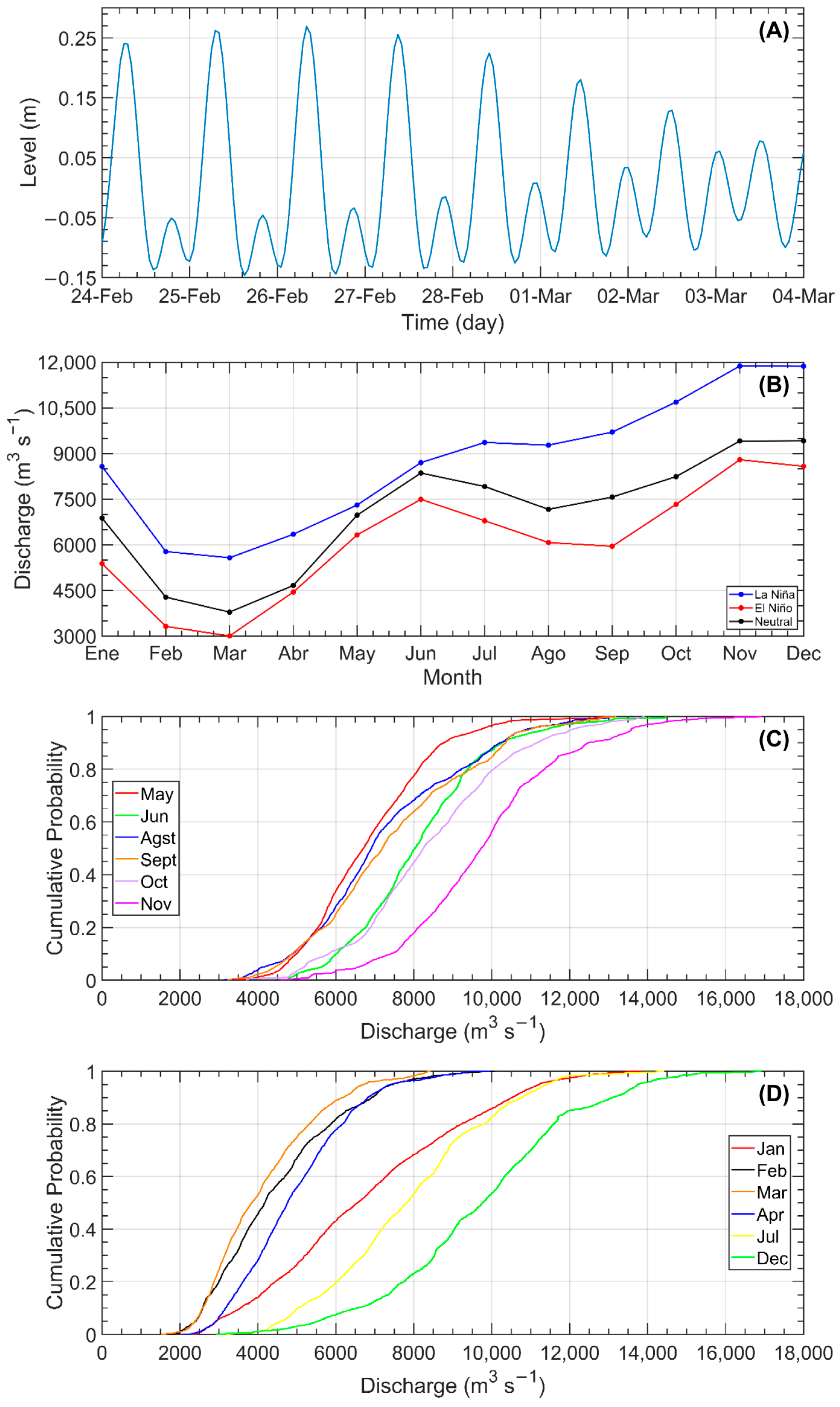
The numerical simulations were performed for spring and neap tidal conditions using water-level forcing extracted from the global FES (Finite Element Solution) 2012 model and prescribed at the open sea boundary as a time-varying boundary condition. Therefore, the tidal scenarios were not imposed as fixed still-water initial levels, but as temporal tidal signals at the ocean boundary. The tidal series shown in Figure 2A spans from 24 February to 4 March 2018 and includes the spring and neap windows selected for the analysis. The spring-tide condition was analyzed from 27 February 2018 00:00 to 28 February 2018 00:00, whereas the neap-tide condition was analyzed from 3 March 2018 00:00 to 4 March 2018 00:00. These windows correspond to representative spring and neap tidal conditions, with tidal ranges of approximately 0.40 m and 0.16 m, respectively. For each scenario, the first five days of simulation were used as spin-up and excluded from the analysis to reduce the influence of initial-condition transients. This spin-up and analysis strategy follows previous approaches [12,32], which showed that short simulation periods are sufficient to achieve quasi-steady-state conditions in the MRE, given its relatively short flushing time under the modeled discharge range. The initial water level was defined by the FES2012 elevation at the start of each simulation, and no artificial water-level offset was applied between scenarios.

Wind waves were not included in the present simulations. The field observations used in the previous model-validation studies were not corrected to remove wave effects and therefore represent the actual environmental conditions present during the campaigns. However, [35] showed that the influence of waves on velocity and salinity is concentrated primarily within the first 2 km upstream of the river mouth, by which point wave energy is reduced by about 95% and the wave-induced change in salinity remains below 2%. Therefore, wave effects are expected to be limited in the upstream stratified region where the TMZ develops under low-discharge conditions.

3.2. Modeling Scenarios

The selected scenarios consist of eight discharge cases under neap tides and eight under spring tides, for a total of sixteen scenarios. To determine the discharges to be simulated, the time series from the Institute of Hydrology, Meteorology and Environmental Studies (IDEAM) was analyzed. The river discharge time series corresponds to daily averages measured from 1940 to 2015 at the Calamar station.

To examine the variability of river discharge in the Magdalena River, climatological means were calculated according to ENSO phase (Figure 2B), using the Oceanic Niño Index (ONI) provided by the National Oceanic and Atmospheric Administration (NOAA). During the cold phase, discharges increase as a result of enhanced precipitation, whereas the opposite occurs during the warm phase, when precipitation decreases. Under La Niña conditions, discharges increase by an average of 26 percent, while under El Niño conditions they decrease by 14 percent.

The river discharge time series was used to compute the monthly cumulative probability distribution for the wet season (Figure 2C) and the dry season (Figure 2D). In the wet season, the highest discharges occur in November, when 80 percent of the time discharge values exceed 8130 m³ s⁻¹. In contrast, during the dry season, the lowest discharges occur in March, with discharge values less than or equal to 5315 m³ s⁻¹ for 80 percent of the time. Discharges less than or equal to 2500 m³ s⁻¹ occur only in February, March, and April, with cumulative probabilities of 7.34 percent, 7.65 percent, and 0.87 percent, respectively.

From the river discharge variability analysis, it was determined that the numerical modeling scenarios would range from 2000 m³ s⁻¹, representing a minimum discharge, and increase in increments of 500 m³ s⁻¹ up to 5500 m³ s⁻¹, since at this value the salt wedge no longer extends beyond km 3 of the estuary [34].

To compute the SSC used in the numerical simulations for each discharge scenario, the sediment discharge (Qs) was obtained in t day⁻¹ from Equation (3) proposed by [28].

$$Qs=1000\times \left[\right(5.7\pm 0.4)\times {10}^{-4}] Q^{1.51\pm 0.01}$$

(3)

To obtain the SSC, Equation (4) from [53] was applied:

$$Qs=Q \times SSC \times k$$

(4)

where Qs is the sediment discharge, Q is the river discharge, SSC is the suspended-sediment concentration, and k = 0.0864 is a unit-conversion coefficient when Qs is expressed in t day⁻¹, Q in m³ s⁻¹, and SSC in mg L⁻¹. For each scenario, Q was prescribed and Qs was estimated from Equation (3). Therefore, SSC was the only unknown and was calculated by solving Equation (4) for SSC.

The resulting sediment discharge and inflow SSC values prescribed at the upstream river boundary for each discharge scenario are summarized in

Table 2. River discharge scenarios and inflow SSC values prescribed at the upstream boundary.

Q (m3 s−1)	Qs (t day−1) [Equation (3)]	SSC (mg L−1) [Equation (4)]	Tide
2000	55,009	318	Neap/spring
2500	77,049	357	Neap/spring
3000	101,468	391	Neap/spring
3500	128,061	423	Neap/spring
4000	156,670	453	Neap/spring
4500	187,165	481	Neap/spring
5000	219,442	508	Neap/spring
5500	253,409	533	Neap/spring

.

3.3. Analysis of Variables and Calculation of Stratification and Mixing Parameters

For the analysis of the numerical modeling results, the thalweg of the MRE was used as the longitudinal reference line (red line in Figure 1A). Along this thalweg, velocity, salinity, and suspended-sediment concentration profiles were extracted, and stratification and mixing parameters were computed by averaging over the selected 24 h analysis windows after spin-up. Additionally, the density field produced by the numerical simulations was corrected using Equation (5) [54], so that the density matrix used to compute the parameters accounted for the suspended-sediment concentration, according to the following expression:

$${\rho }_{= }{\rho }_w+\left(1-{\displaystyle \frac{{\rho }_w}{{\rho }_{sed}}}\right) \times SSC$$

(5)

where ${\rho }_w$ is the density of estuarine water and ${\rho }_{sed}$ is the particle density of the suspended sediment, assumed constant in the density-correction calculation and set to 2600 kg m⁻³. Equation (5) was applied element by element to the time-averaged longitudinal-vertical density field along the thalweg, using the corresponding time-averaged SSC value. Subsequently, the stratification parameter (ε), the layer Richardson number (R_i), and the turbulent kinetic energy production (P) were calculated.

• Stratification parameter (ε)

This parameter accounts for the density difference between the surface and the bottom and is calculated as follows:

$$\mathsf{\epsilon }={\displaystyle \frac{\partial \rho }{{\rho }_0}}$$

(6)

$$\partial \rho ={\rho }_b-{\rho }_s$$

(7)

where ${\rho }_b$ is the density at the bottom, ${\rho }_s$ is the density at the surface, and ${\rho }_0=0.5\times ({\rho }_b+{\rho }_s)$. When $\epsilon$ is close to 0, the water column is well mixed, whereas values near 0.025 indicate stratification and the presence of a salt wedge [55].

• Richardson number (${\mathrm{R}}_{\mathrm{i}}$)

This dimensionless parameter compares the stability of the water column resulting from buoyancy forces with the shear stress, allowing an estimation of the intensity of mixing [56].

$$R_i={\displaystyle \frac{gh\left(\rho b-\rho s\right)}{U^2\rho o}}$$

(8)

$U$ is the depth-averaged velocity, $\rho o$ is the depth-averaged density, $h$ is the water depth, $\left(\rho b-\rho s\right)$ is the density difference between the bottom and the surface, and $g$ is gravitational acceleration. Ref. [57] found that for $R_i$ $\ge$ 20 bottom-generated turbulence is not sufficient to overcome stratification, for 20 $>$ $R_i$ $>$ 2, mixing becomes increasingly effective and for R_i ≤ 2, the water column is well mixed.

• Turbulent kinetic energy production ($\mathrm{P}$)

It refers to the production of turbulence resulting from the interaction between mean shear stress and Reynolds stresses. It represents the intensification of eddies as they are stretched by the mean shear [58]. Near the bottom, this parameter is calculated using the following equation:

$$P\cong {\displaystyle \frac{u_{\ast }^3}{kz}}$$

(9)

where k is the von Kármán constant (≈0.41) and ${\mathrm{u}}_{\ast }$ is the bottom shear velocity, which is calculated as follows:

$$u_{\ast }^2=C_d\times u_1^2$$

(10)

where $Cd$ is the drag coefficient, set to 0.18 in this study, and $u_1$ is the velocity in the first cell above the bed in the model [27].

From the numerical simulation outputs, two metrics of suspended-sediment concentration were defined for the analysis. The first, SSC_max, corresponds to the absolute maximum SSC value identified anywhere within the longitudinal-vertical profile along the thalweg of the MRE (i.e., at any depth and any distance from the mouth). This metric captures the peak concentration associated with the TMZ core in the vertical plane. The second, $\overline{\mathrm{SSC}}$, corresponds to the depth-averaged SSC computed at each point along the thalweg. Its maximum value along the thalweg, ${\overline{\mathrm{SSC}}}_{\max }$, identifies the position and magnitude of the TMZ core as seen from a vertically integrated perspective, which is more directly comparable with surface-based observations and relevant for navigation-channel management.

3.4. Analysis of Salt-Wedge Dynamics and the TMZ

Once the results were processed, the maximum extent of the salt wedge was determined as the farthest point upstream where ε > 0 along the thalweg. The TMZ core position was defined as the distance from the mouth where ${\overline{\mathrm{SSC}}}_{\max }$ occurs. Subsequently, the positions of the FSI and the TMZ core were compared across all scenarios to establish their relationship and to identify the value of ε at which the TMZ core consistently forms. Although sixteen scenarios were simulated, the results are presented in detail for four representative discharge cases (Q = 2000, 3000, 4000, and 5000 m³ s⁻¹), which span the full range of salt-wedge behavior, from maximum intrusion under extreme low-flow conditions to confinement at the mouth.

4. Results

4.1. SSC, Velocity, and Salinity Profiles

Before presenting the results, it is important to distinguish between the two SSC metrics used in the analysis. SSC_max refers to the absolute local maximum SSC identified at any depth and distance along the longitudinal-vertical profile, whereas ${\overline{\mathrm{SSC}}}_{\max }$ refers to the maximum value of the vertically averaged SSC along the thalweg. Therefore, SSC_max represents a local concentration peak, while ${\overline{\mathrm{SSC}}}_{\max }$ represents the vertically integrated expression of the TMZ core.

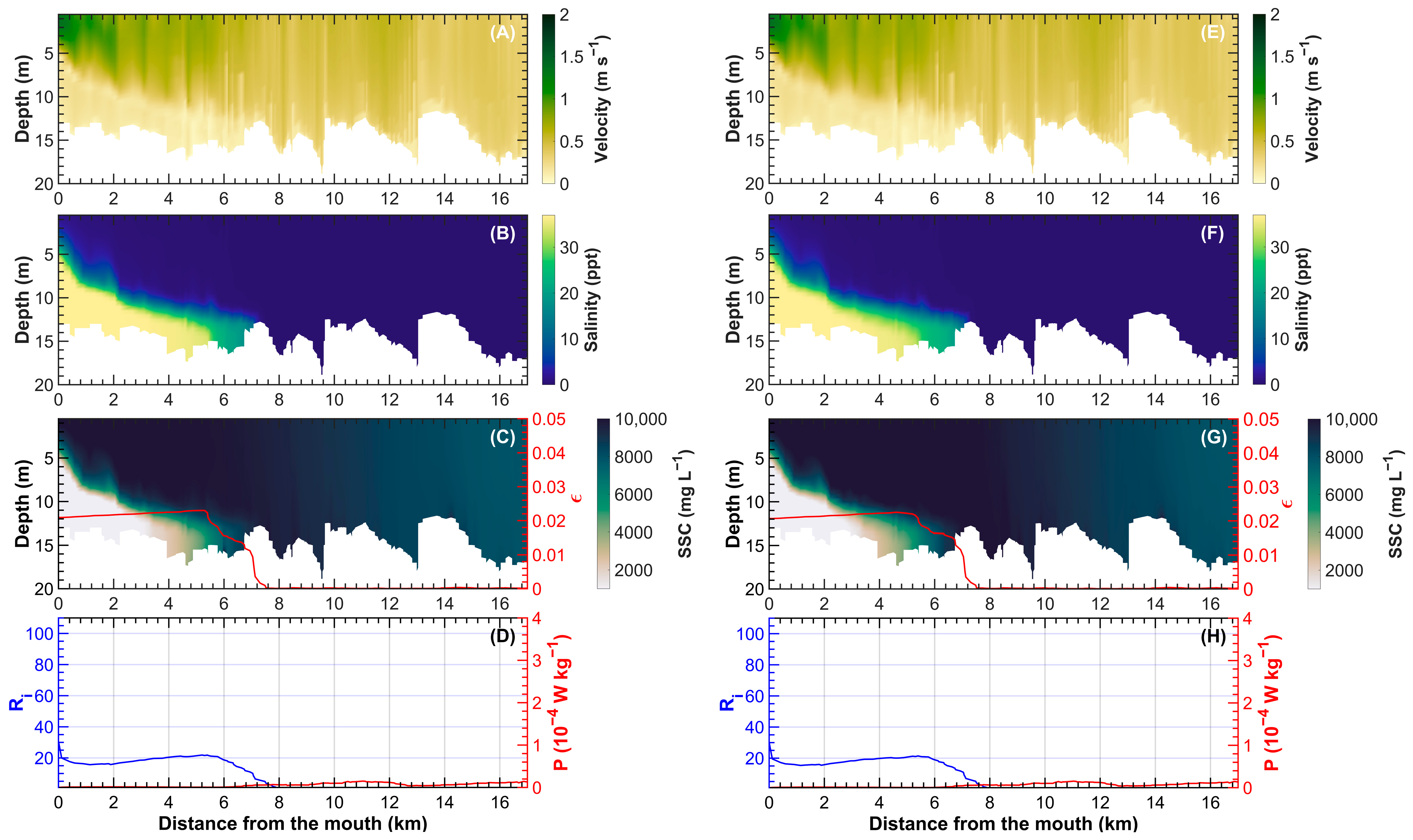
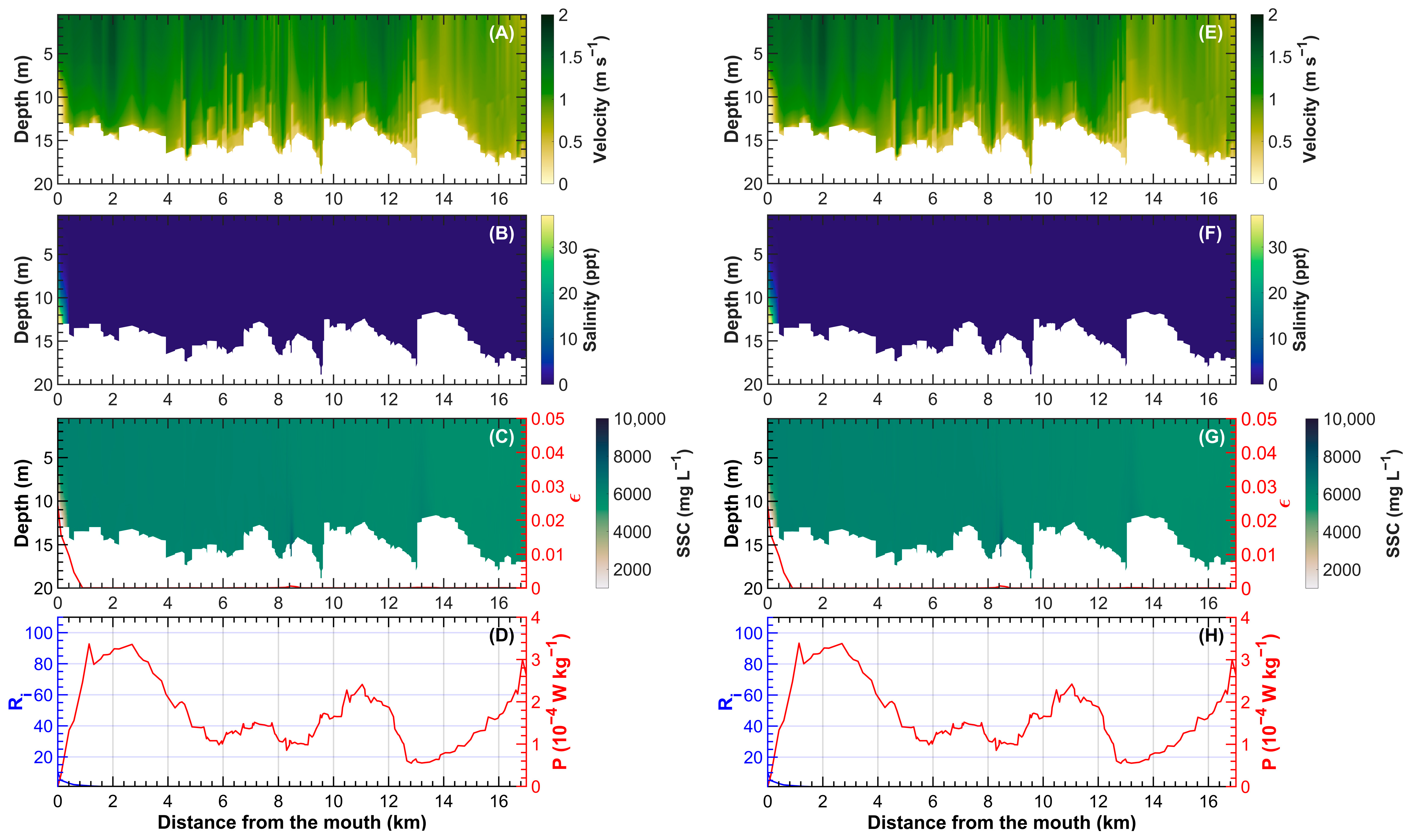
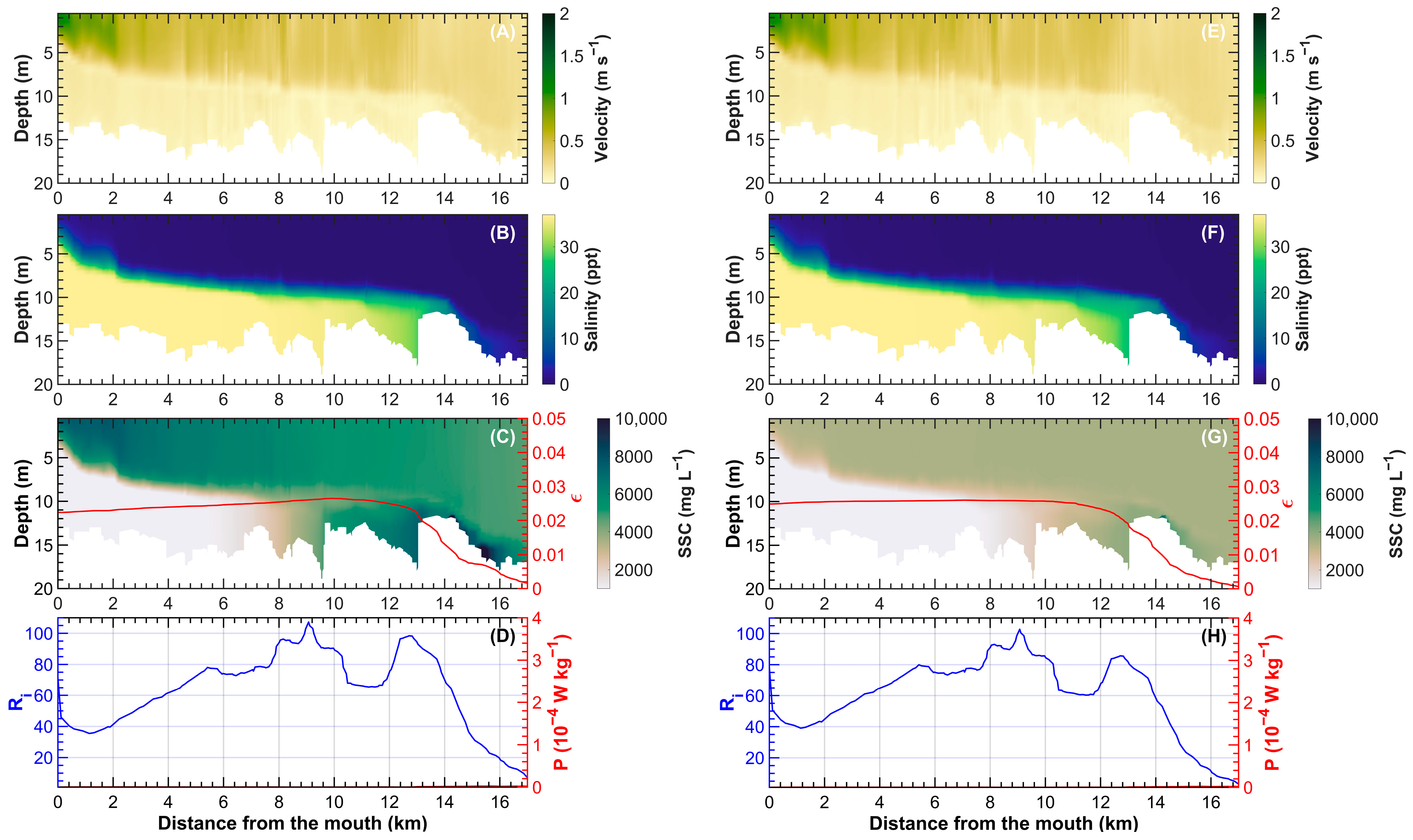
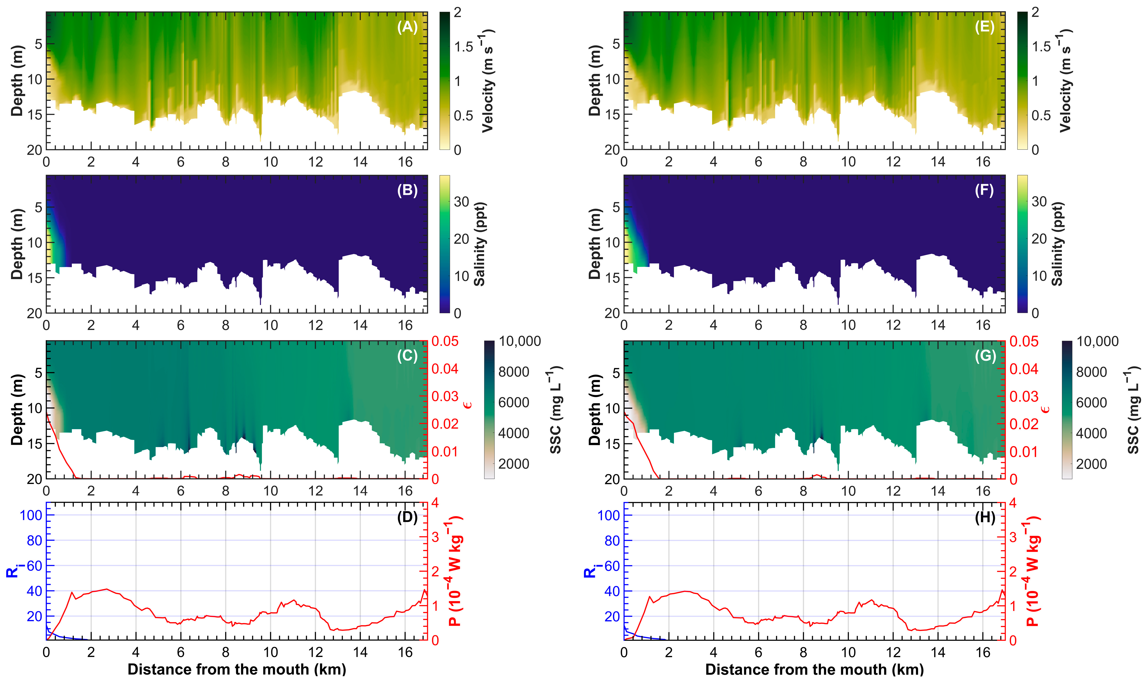
From Figure 3, Figure 4, Figure 5 and Figure 6, the velocity, salinity, and SSC profiles are shown together with the stratification and mixing parameters for eight modeled scenarios. Although sixteen scenarios were considered, only the most relevant results are presented due to space constraints. As river discharge increases, the penetration length of the salt wedge decreases. For all velocity profiles, it is evident that velocity approaches values near zero at the convergence front associated with the salt wedge and increases toward the mouth. The salt wedge is identified by its lower SSC values, whereas in the fluvial section suspended-sediment concentrations are higher.

Table 3. Summary of key parameters from longitudinal-vertical profiles for selected discharge scenarios.

Q (m3 s−1)	Tide	Salt Wedge Extent (km)	SSCmax (mg L−1)	Higher-SSC Zone/SSCmax Location (km)	Ri ≥ 20 Extent (km)	Pmax (W kg−1)
2000	Neap	>17	15,500	14.2	0–16	≈0
2000	Spring	>17	8750	14.2	0–15.5	≈0
3000	Neap	~7.6	10,300	mouth–km 10	0–5.5	increases from km 8
3000	Spring	~7.6	9000	mouth–km 10	0–5.5	increases from km 8
4000	Neap	~1.5	6450	0–1	—	1.5 × 10−4 (km 1–4)
4000	Spring	~1.5	6100	mouth	—	1.5 × 10−4 (km 1–4)
5000	Neap	<1	6150	mouth	—	3.4 × 10−4 (km 1–3)
5000	Spring	<1	6150	mouth	—	3.4 × 10−4 (km 1–3)

summarizes the key hydrodynamic and sediment-transport parameters extracted from the longitudinal-vertical profiles (Figure 3, Figure 4, Figure 5 and Figure 6) for the four representative discharge scenarios under both tidal conditions.

Three main trends emerge from these profiles. First, as river discharge increases from 2000 to 5000 m³ s⁻¹, the salt wedge retreats progressively from beyond km 17 to less than km 1, and the zone where R_i ≥ 20 (indicating that bottom-generated turbulence is insufficient to overcome stratification) contracts accordingly. Second, SSC_max decreases with increasing discharge despite the higher solid discharge, because the weakening of stratification at higher flows reduces the efficiency of the sediment trap. Third, the neap-spring tidal contrast in SSC is most pronounced at Q = 2000 m³ s⁻¹, where SSC_max under neap tide (15,500 mg L⁻¹) is 77% higher than under spring tide (8750 mg L⁻¹). This difference diminishes as discharge increases: at Q = 3000 m³ s⁻¹ the neap-spring contrast is approximately 14%, and at Q ≥ 4000 m³ s⁻¹ it becomes negligible. This pattern is consistent with the progressive suppression of turbulent kinetic energy production (P ≈ 0) under low-discharge conditions, which allows the salt wedge to act as a highly efficient sediment trap during neap tides, when tidal mixing is further reduced.

4.2. Dynamics of the TMZ and the FSI

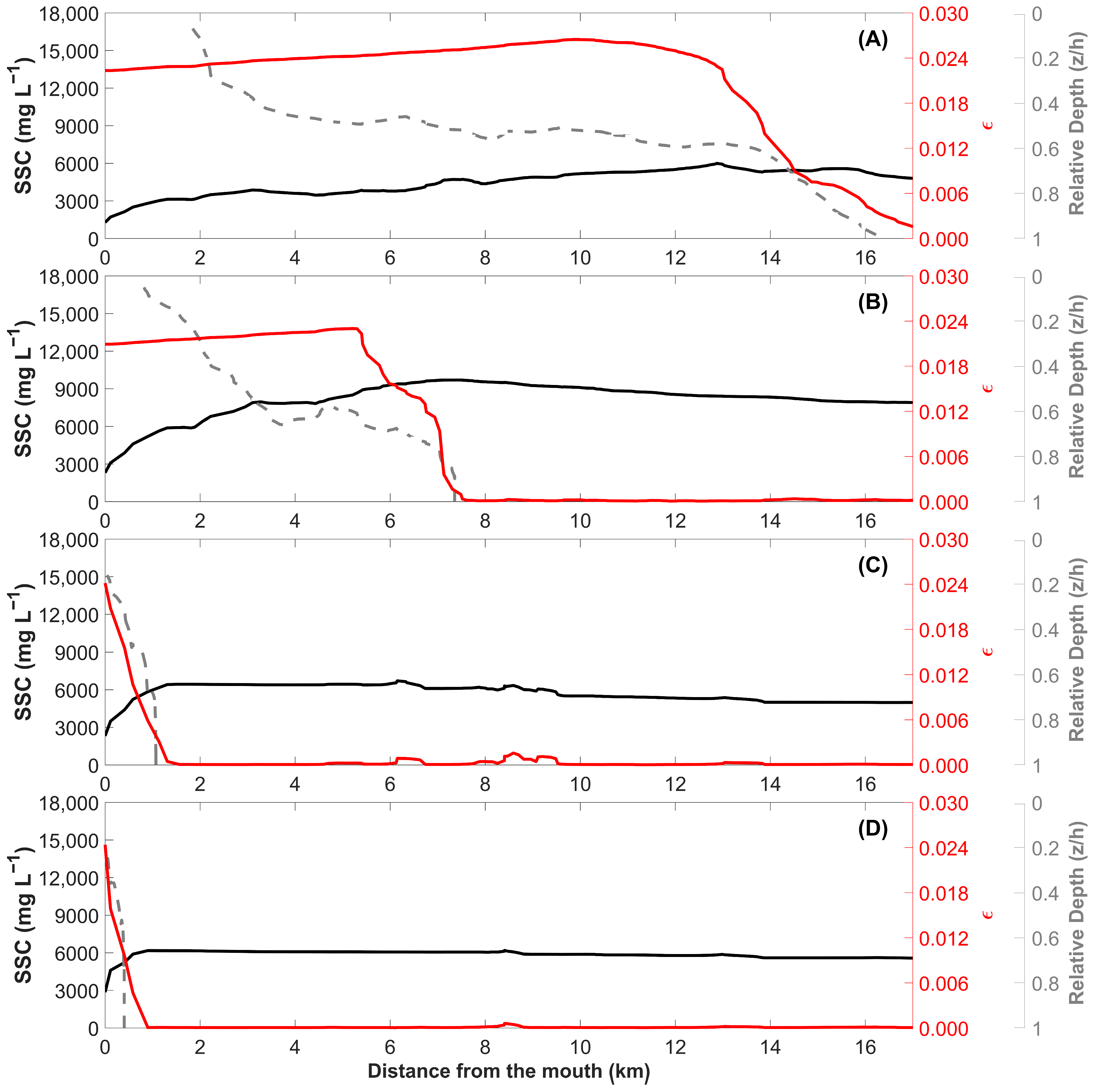
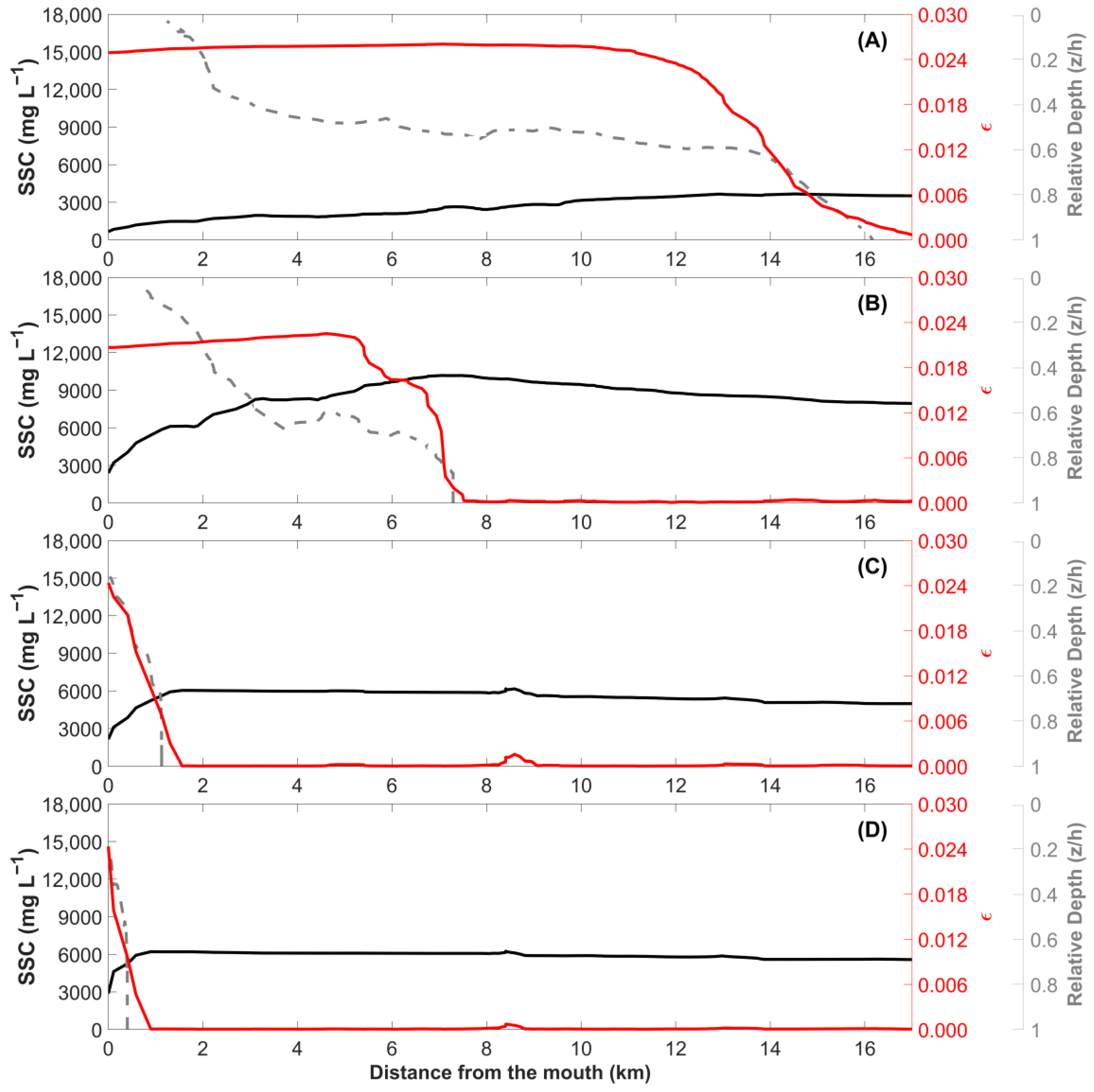
In Figure 7 and Figure 8, the vertically averaged SSC ($\overline{\mathrm{SSC}}$), the stratification parameter, and the 1-ppt isohaline are shown for the representative scenarios under neap and spring tides, respectively. For both tidal conditions, the highest vertically averaged SSC values (${\overline{\mathrm{SSC}}}_{\max }$) occur for Q = 3000 m³ s⁻¹. It is also observed that the longitudinal position where $\overline{\mathrm{SSC}}$ reaches its maximum follows a trend similar to the position where ε crosses the value of 0.005 (

Table 4. Maximum vertically averaged SSC (${\overline{\mathrm{SSC}}}_{\max }$), TMZ core position, and position where ε = 0.005 for representative discharge and tidal scenarios.

Q (m3 s−1)	Tide	${\overline{\mathbf{SSC}}}_{\mathbf{max}}$ (mg L−1)	TMZ Core Position (km)	ε = 0.005 Position (km)	Δ (km)
2000	Neap	5990	13.00	16.00	−3.0
2000	Spring	3660	14.80	15.00	−0.2
3000	Neap	9700	7.50	7.10	0.4
3000	Spring	10,170	7.10	7.10	0.0
4000	Neap	6440	1.60	0.90	0.7
4000	Spring	6040	1.50	1.20	0.3
5000	Neap	6170	0.90	0.60	0.3
5000	Spring	6200	0.90	0.60	0.3

).

Table 4 presents the maximum vertically averaged SSC (${\overline{\mathrm{SSC}}}_{\max }$), the position of the TMZ core, and the position where ε = 0.005 for the representative scenarios.

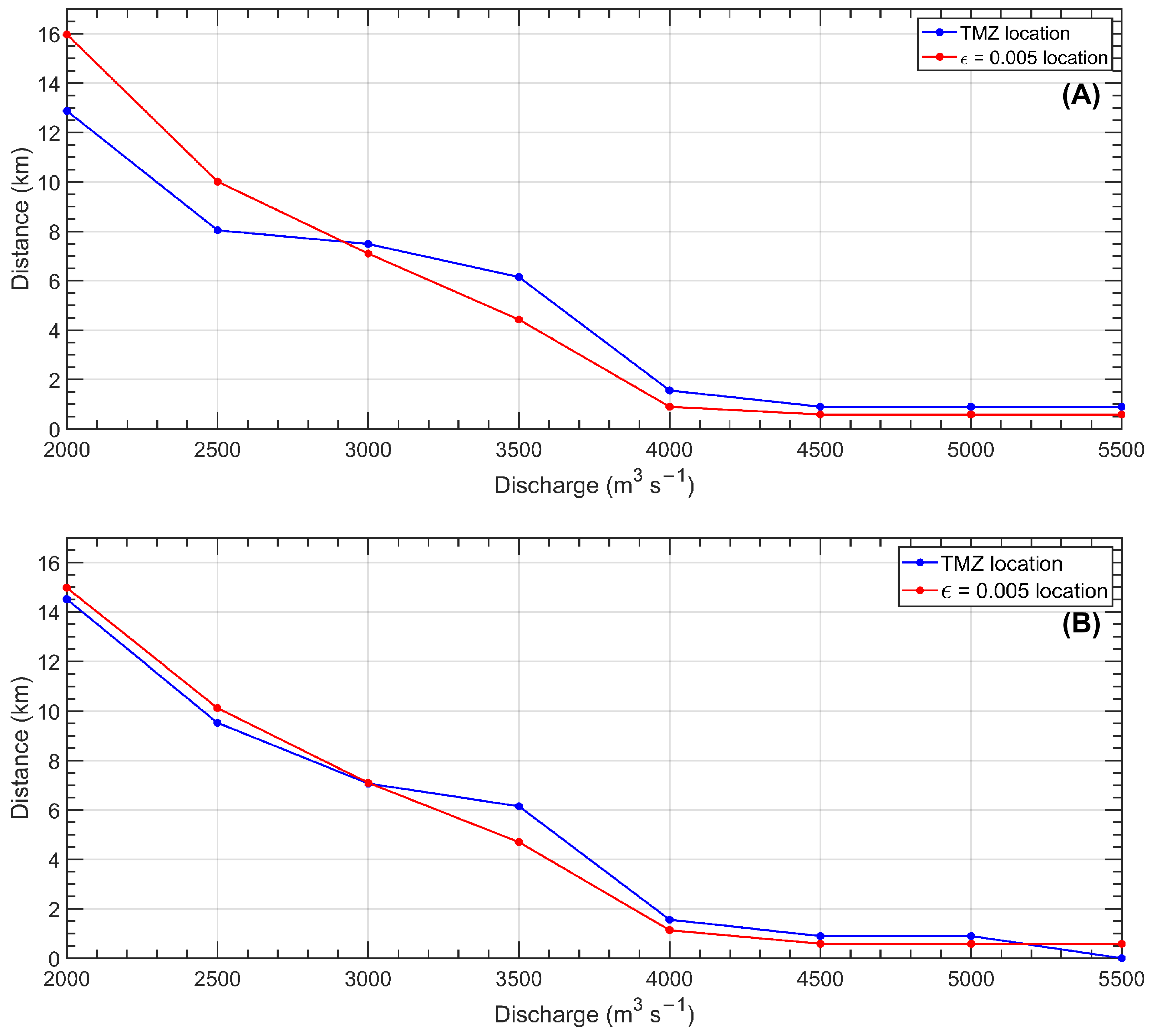
As discharge increases, the TMZ core shifts progressively from km 13–15 for Q = 2000 m³ s⁻¹ to km 0.9 for Q = 5000 m³ s⁻¹. The position where ε = 0.005 follows the same trend, with a coefficient of determination of R² = 0.96 and an RMSE of 1.1 km between the two positions across all sixteen scenarios. A systematic offset is observed: for Q = 2000 m³ s⁻¹ under neap tide, the position where ε = 0.005 is located 3 km upstream of the TMZ core, whereas for Q ≥ 4000 m³ s⁻¹, the TMZ core is located 0.3–0.7 km upstream of the position where ε = 0.005. Under spring tides, the offset is consistently smaller, with an RMSE of 0.46 km. Notably, for Q = 2000 m³ s⁻¹, $\overline{\mathrm{SSC}}$ under neap tide is 64% higher than under spring tide, whereas for Q ≥ 3000 m³ s⁻¹ this contrast diminishes or reverses.

The contrast between SSC_max and ${\overline{\mathrm{SSC}}}_{\max }$ suggests a change in the vertical structure of the sediment trap between low-discharge scenarios. Under Q = 2000 m³ s⁻¹, the highest sediment concentrations occur near the bed, producing the largest local SSC_max. In contrast, under Q = 3000 m³ s⁻¹, sediment is distributed over a thicker portion of the water column, which increases ${\overline{\mathrm{SSC}}}_{\max }$ even though the local peak concentration is lower.

In these profiles, it is also observed that the FSI, defined following [14] as the point where the 1-ppt isohaline intersects the channel bed, is located downstream of the position where ε becomes zero, and ${\overline{\mathrm{SSC}}}_{\max }$ occurs in close proximity to this location for all cases.

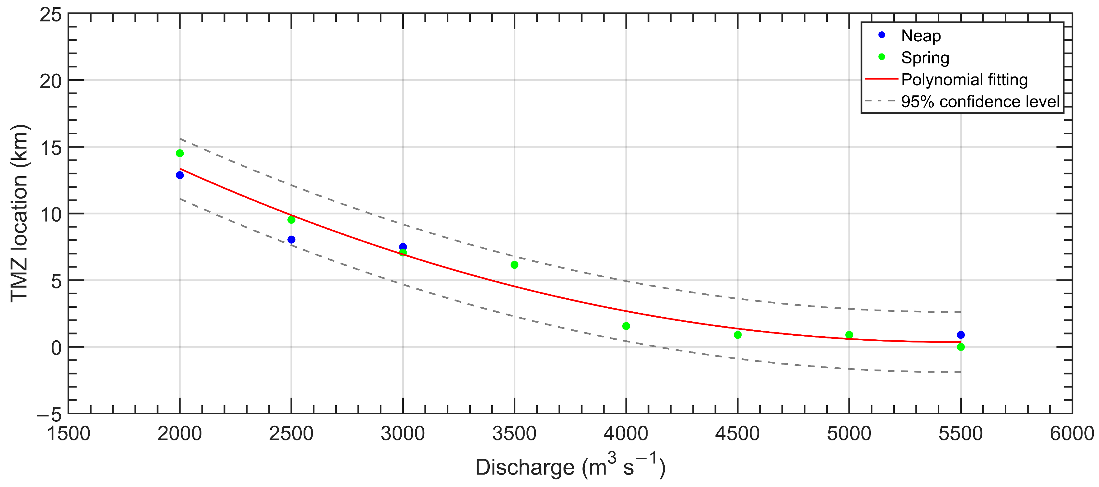
In Figure 9, the position of the TMZ core is shown, defined as the location where ${\overline{\mathrm{SSC}}}_{\max }$ occurs, together with the position where ε = 0.005 for each discharge scenario. As river discharge increases, both the TMZ and the reduction in ε occur progressively closer to the mouth. Although the two positions do not coincide exactly, both follow the same decreasing trend with discharge, confirming that the position where ε = 0.005 is a first-order spatial predictor of the TMZ core position across the full range of modeled scenarios.

5. Discussion

5.1. Effect of Tides on Salt-Front Dynamics and the Dynamics of the Estuarine Turbidity Maximum

The position of the salt front does not exhibit substantial differences between neap and spring tidal scenarios. This behavior reflects the limited tidal energy available under the microtidal regime of the MRE, where river flow primarily controls the salt-wedge intrusion length and the longitudinal displacement of the TMZ. A similar hierarchy of forcings was observed in the tropical microtidal Jamapa River estuary, where river discharge primarily controlled the salt-wedge position and tidal effects were most evident near the estuary entrance under calm-wind conditions [59]. Episodic wind forcing can temporarily enhance saline intrusion and overwhelm the tidal influence, indicating that short-term meteorological forcing may superimpose additional variability on the discharge-controlled salt-wedge response [59]. In the MRE, however, suspended-sediment concentrations within the estuarine turbidity maximum are clearly influenced by tidal conditions, with higher values occurring during neap tides. This contrast is most pronounced under extreme low-discharge conditions. For Q = 2000 m³ s⁻¹, SSC_max during neap tide (15,500 mg L⁻¹) is 77% higher than during spring tide (8750 mg L⁻¹), while the vertically averaged ${\overline{\mathrm{SSC}}}_{\max }$ is 64% higher (5990 vs. 3660 mg L⁻¹). As discharge increases, this neap-spring contrast diminishes progressively, becoming negligible for Q ≥ 4000 m³ s⁻¹ (Table 4). The effects of increased SSC on stratification become evident from km 12 for the Q = 2000 m³ s⁻¹ scenario, where both ε and R_i increase under neap tides compared with spring tides. This increase in stratification and stability parameters is associated with enhanced near-bed SSC in this sector of the estuary. This is consistent with the fact that suspended sediments contribute to density stratification primarily in bottom layers, whereas stratification near the surface and within intermediate layers is mainly driven by salinity gradients [60].

During neap tides, the reduced amplitude of the tidal wave decreases interfacial turbulent mixing, as evidenced by Richardson number (R_i) values consistently exceeding 20 within the salt-wedge (Figure 3). This hydrodynamic stability has a dual effect. First, it preserves the integrity of the salt wedge, allowing it to penetrate farther upstream or remain stationary. Second, it suppresses vertical mass diffusivity (Kz approaching zero). Under these low-energy conditions, flocculated fine particles settling from the surface freshwater layer become trapped within the lower saline layer. In the absence of sufficient turbulent energy to resuspend them back into the upper layer, and given that near-bed residual velocities are weakly landward, sediments progressively accumulate, leading to the formation of a high-density TMZ.

In addition, sediment-induced stratification can suppress turbulence to a degree that depends on the gradient of suspended-sediment concentration [61]. Ref. [62] showed that in the Yangtze River estuary (China), when the density gradient generated by suspended sediments is taken into account, saline intrusion extends farther upstream during neap tides than during spring tides. In other words, sediments can enhance salt-wedge stability during neap tides by locally strengthening the vertical density gradient. This occurs because tidal mixing is weaker during neap tides and the estuary becomes more strongly stratified, which may explain the increase in SSC observed under these conditions in the Magdalena River Estuary.

Ref. [34] found through numerical simulations in the MRE that salt-wedge intrusion is up to 1 km greater during spring tides. However, their analysis did not consider the contribution of suspended sediments to density, which is a key factor in highly turbid estuaries. The lack of marked differences in salt-wedge penetration length between spring and neap tides observed in the present study may be attributed to the reduction in tidal mixing during neap tides, which promotes stratification superimposed on the smaller tidal range characteristic of these conditions. This combined effect acts in the opposite sense, damping salt-wedge penetration and, consequently, reducing stratification.

During spring tides, the increase in turbulent kinetic energy (P), although insufficient to fully mix the water column, can erode the pycnocline. This entrainment process transfers sediments from the near-bed trap into the surface layer, where high river velocities export them seaward. In this way, spring tides act as a partial flushing mechanism for the estuary, reducing the amount of stored SSC. This flushing role of spring tides is consistent with the findings of [63] in the Pearl River Estuary, where most riverine sediment was trapped in the estuary during neap tides and only approximately 12% was exported seaward during spring tides. In the York River estuary, ref. [25] showed that the asymmetry in tidal mixing between flood and ebb controls net sediment pumping, with stratification modulating the efficiency of sediment retention. However, a fundamental difference exists between these partially mixed systems and the MRE since in the former, spring tides enhance resuspension and typically increase water-column SSC, whereas in the MRE, the dominant effect of spring tides is the erosion of the pycnocline and the resulting seaward export of trapped sediment, leading to lower SSC within the TMZ. Mixing becomes more intense during the flood phase, when bottom-generated turbulence is enhanced, resulting in increased sediment transport and morphological changes driven by higher turbulent kinetic energy [64].

A crucial aspect revealed by the modeling is the active role of sediments in stratification, suggesting the possible development of lutocline-like or fluid-mud-like near-bed structures, where the self-weight of the sediment suppresses turbulence and inhibits its own resuspension. This positive feedback mechanism explains why stratification persists beyond the theoretical limit of saline intrusion under neap tide conditions (Figure 7A). Sediment in the MRE is not a passive tracer; it is a dynamic agent that modifies the flow field, reinforcing the very trap that retains it. The SSC values within the TMZ under low-discharge conditions (SSC_max up to 15,500 mg L⁻¹ for Q = 2000 m³ s⁻¹) place the MRE within the range of hyperturbid systems [65], comparable to the Yellow River where sediment-induced stratification has been shown to dominate over salinity-induced stratification. This distinguishes the MRE from lower-turbidity estuaries where salinity gradients alone govern the vertical density structure and where tidal resuspension, rather than stratification-controlled trapping, determines the neap-spring variability of SSC.

5.2. Effects of River Discharge on the Dynamics of the FSI and the TMZ

River discharge in the Magdalena River varies seasonally, with the lowest discharges occurring in March during the dry season and the highest in November during the wet season. At interannual timescales, however, discharge is also influenced by the dominant phase of ENSO. In this study, it was found that for discharges below 5000 m³ s⁻¹, the estuary remains stratified beyond km 0 and mixing is not efficient enough to break stratification. These discharge conditions are common during the dry season under warm and neutral ENSO phases. For discharges of 4000 m³ s⁻¹ and 5000 m³ s⁻¹, the salt wedge becomes restricted to the first 2 km of the estuary due to enhanced mixing driven by increased turbulence, as reflected by higher values of turbulent kinetic energy production (P) under these scenarios. These results are consistent with [29], who found that for a discharge of 6000 m³ s⁻¹ the salt wedge is located around km 1 of the estuary. When discharge decreases from 4000 to 3500 m³ s⁻¹, saline intrusion shifts from km 1.5 to km 5.5, highlighting its strong sensitivity to river discharge [40]. A similarly strong discharge control has been reported for the microtidal Neretva River estuary, where river inflow was identified as the dominant driver of salt-wedge dynamics, whereas tides and sea-level variations mainly produced comparatively small short-term fluctuations [66]. The relationship between salt-wedge length and river discharge may change across discharge ranges because of constraints imposed by channel geometry [66].

Considering the analysis of the river discharge time series, the salt wedge is expected to reach its maximum penetration length during the warm ENSO phase in the dry season. Under these conditions, discharge can decrease to values as low as 2000 m³ s⁻¹, allowing the salt wedge to extend beyond km 17. Ref. [29] determined that under this scenario stratification reaches up to km 21. Accordingly, the TMZ is expected to develop around this location, increasing SSC and promoting sedimentation in this sector of the estuary. In addition, under these conditions turbulent kinetic energy production (P) is nearly zero, further favoring sediment settling.

These findings are comparable to those reported by [12], who analyzed bathymetric data from different years and found that in 2016 the highest sedimentation occurred during the March to February period, with a rate of 883 mm per year. It is noteworthy that the ONI for the dry season of 2016 indicates El Niño conditions, during which river discharge values in February and March ranged between 2500 and 3000 m³ s⁻¹. Under these conditions, enhanced sedimentation would be expected to occur between km 4 and km 14 of the estuary.

Sedimentation also predominated during the August to July period, with a rate of 271 mm per year. As shown in Figure 2, river discharge decreases during these months due to the Veranillo de San Juan. This reduction in discharge can lead to an increase in SSC within the estuary, thereby promoting sedimentation as river flow weakens. However, climatological mean river discharge values for these months remain above 6000 m³ s⁻¹, suggesting that the salt front is likely located near the mouth or farther offshore.

For the cold ENSO phase and during the wet season under neutral and warm ENSO conditions, ref. [29] found that the salt wedge remains restricted to the mouth, as river discharges exceed 4000 m³ s⁻¹. Ref. [12] determined that the periods with the highest erosion rates in 2016 were February to January, September to August, October to September, November to October, and December to November, with rates ranging from 194 mm per year for October to September to 952 mm per year for February to January. These months generally coincide with periods of higher river discharge, except for the February to January interval. Under such conditions, the salt wedge retreats and sediments are exported from the estuary toward the delta front. During the February to January period, river competence decreases as discharge is reduced, causing suspended material to settle and migrate toward the salt front [34].

The turbulent kinetic energy production (P) and the Richardson number (R_i) provide useful estimates of bottom shear stress $\left({\tau }_{xy}\right)$, with P being directly proportional to ${\tau }_{xy}$, and R_i inversely proportional to ${\tau }_{xy}$ [34]. At higher discharges, increased P values and reduced R_i lead to larger ${\tau }_{xy}$, favoring erosion along the navigation channel.

In the velocity profiles, a reduction in flow velocity is observed at the freshwater–saltwater interface, where the halocline is located. This reduction results from the convergence of two opposing flows, riverine and marine, as previously reported by [29]. The decrease in velocity also contributes to sediment settling by drastically reducing turbulent kinetic energy within the estuary.

In addition, velocities increase near the mouth above the salt wedge due to the reduction in the channel cross-sectional area in this zone. Upstream, velocity reductions are associated with channel widening, as occurs around km 14, or because the thalweg deviates toward shoals, where velocities are lower due to enhanced friction along the channel margins.

Near the FSI, suspended-sediment concentrations increase as the stratification parameter decreases. Because suspended sediments contribute to density, the high SSC present at the salt front at near-bed depths prevents the complete reduction in the stratification parameter ε. As a result, the zone of maximum SSC along the longitudinal section and the location of the peak $\overline{\mathrm{SSC}}$ do not coincide exactly with the position where ε becomes zero. Instead, the TMZ core forms at a longitudinal position that tracks the location where ε = 0.005 (R² = 0.96, RMSE = 1.1 km; Table 4, Figure 9). The offset between the two positions varies systematically with discharge and tidal conditions, so that under low-discharge neap conditions (Q = 2000 m³ s⁻¹), the location where ε = 0.005 is approximately 3 km upstream of the TMZ core, which is consistent with the fact that under extreme stratification the sediment trap extends over a broader zone and the TMZ core is displaced downstream relative to the stratification front. Under spring tides, the offset is minimal (<1 km) across all discharges, likely because enhanced tidal mixing compresses the transition zone between stratified and mixed conditions. These results also demonstrate that when sediment effects are accounted for, stratification in the estuary persists beyond the salt front [62].

For the SSC profiles, although solid discharge is lower under reduced river discharge conditions, SSC values are higher. This occurs because stratification weakens vertical mixing, thereby promoting flocculation and the settling of suspended sediments [14,67]. This behavior is evidenced by the fact that turbulent kinetic energy production (P) is nearly zero under these scenarios, favoring an increase in SSC within the riverine section. As was mentioned in Section 2, the SSC threshold of 4500 mg L⁻¹ proposed by [14] to delimit the TMZ was derived from field campaigns conducted under a specific discharge condition (Q ≈ 4500 m³ s⁻¹). The present numerical results confirm that this threshold is not generalizable because ${\overline{\mathrm{SSC}}}_{\max }$ across the simulated scenarios ranges from 3660 mg L⁻¹ (Q = 2000 m³ s⁻¹, spring tide) to 10,170 mg L⁻¹ (Q = 3000 m³ s⁻¹, spring tide), varying by nearly threefold depending on discharge and tidal conditions (Table 4). The functional criterion adopted in Section 3—locating the TMZ core at the position of maximum $\overline{\mathrm{SSC}}$ —avoids this dependence and enables consistent identification of the TMZ across all scenarios. For the highest modeled discharges, sediment export from the estuary toward the ocean is enhanced [63].

This behavior is similar to that reported by [42] for the Yalu River estuary in China. As river discharge increases, the salt front shifts seaward and estuarine circulation becomes confined to the lower estuary, trapping large amounts of sediment downstream of the flow null point and contributing to the formation of the TMZ. The flow null point corresponds to the location where landward near-bed flow converges with seaward river-driven transport occurring in the upper layers.

The results show a nonlinear inverse relationship between river discharge and the position of the TMZ. Figure 10 illustrates a polynomial fit between these two variables, yielding a coefficient of determination R² = 0.976 for

$$TMZ\left(Q\right)=1.0096\times {10}^{-6}{Q}^2-0.0115Q+34.1767$$

(11)

where $TMZ\left(Q\right)$ is the distance from the estuary mouth (in km) at which the TMZ core is located, and Q is the river discharge (in m³ s⁻¹). This equation is valid for the range 2000 ≤ Q ≤ 5500 m³ s⁻¹. This equation is similar to that proposed by [34] to establish the relationship between river discharge and the position of the FSI:

$$FSI\left(Q\right)=1.133\times {10}^{-6}{Q}^2-0.0142Q+46.2825$$

(12)

This demonstrates that the dynamics of the TMZ are closely linked to the position of the FSI. The proposed equation provides a first-order approximation for predicting the location of the TMZ and, consequently, the areas within the MRE where sedimentation is likely to intensify.

Moreover, the position where ε = 0.005 constitutes a robust first-order predictor of the TMZ core location within the MRE (R² = 0.96; Figure 9, Table 4), with an overall accuracy of ±1.1 km. Physically, in the MRE this value of the stratification parameter marks the zone where buoyancy begins to dominate over fluvial inertia, and the TMZ core forms in its vicinity because this transition concentrates the mechanisms of sediment trapping, including suppression of turbulence, convergent near-bed flow, and enhanced flocculation. Upstream of this point (ε < 0.005), the flow is essentially fluvial and turbulent, maintaining sediments in suspension. Downstream, stratification damps turbulence, facilitating rapid sedimentation. This result has direct practical implications for dredging engineering. Unlike the 1-ppt isohaline, which can be highly mobile and difficult to monitor in real time throughout the water column, the parameter ε integrates the full density structure of the estuary. The derived polynomial relationship between river discharge Q and the position of the TMZ suggests that dredging efforts should be dynamically relocated. During El Niño phases (Q < 3000 m³ s⁻¹), critical sedimentation zones shift landward toward the reach between km 13 and km 18, affecting port maneuvering areas that are typically free of sedimentation issues. During La Niña conditions, sedimentation is concentrated exclusively at the mouth (Bocas de Ceniza), requiring intensified operations within a geographically limited but hydrodynamically complex area.

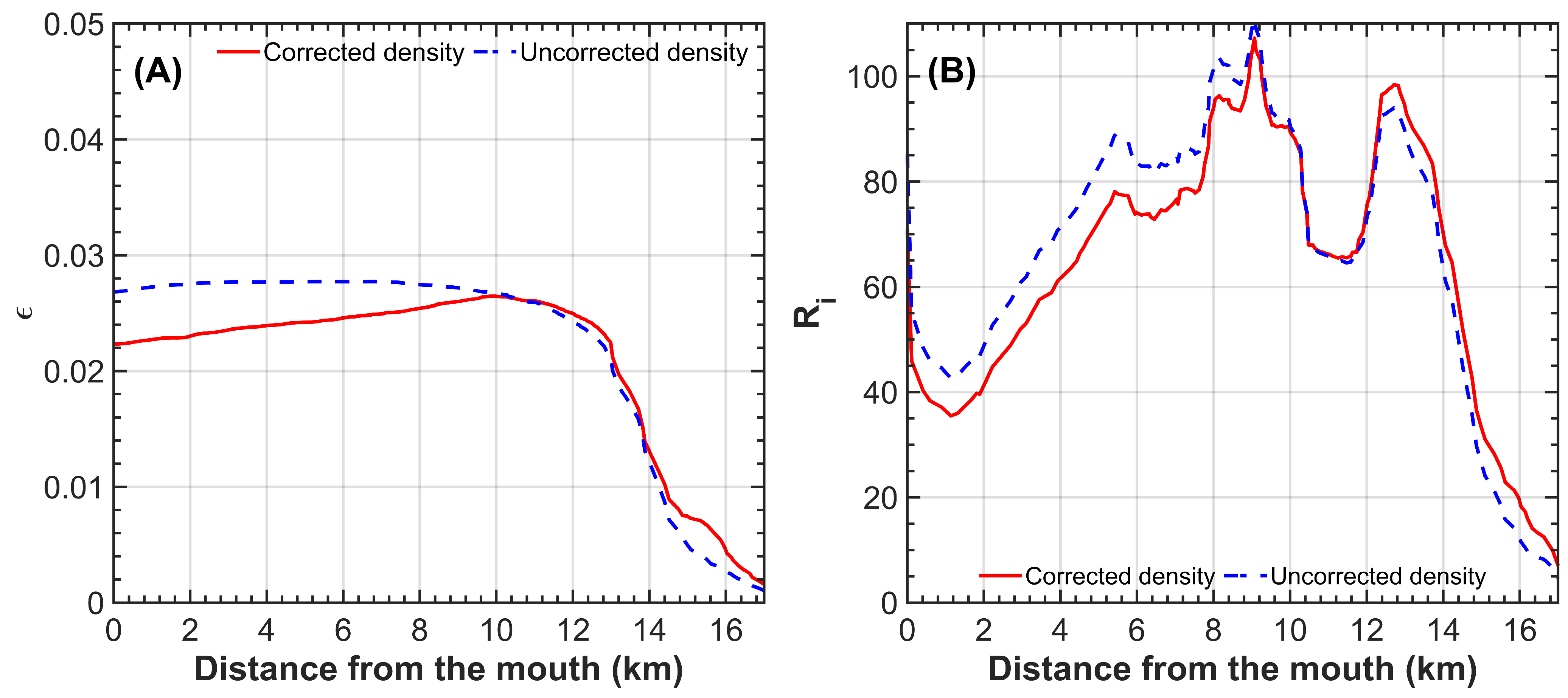
To further examine the role of sediment-induced density effects, a diagnostic comparison was performed for the Q = 2000 m³ s⁻¹ scenario by computing ε and Ri with and without the sediment-density correction (Figure 11). The results indicate that the sediment contribution to stratification is spatially variable. Downstream of the TMZ core, where salinity-driven stratification dominates, the sediment-density correction increases the density of the sediment-rich fluvial layer. As expected, this weakens the vertical density gradient between the riverine layer and the saline lower layer, leading to locally lower ε and Ri values compared with the uncorrected-density case. In contrast, near and upstream of the TMZ core, the sediment-density correction increases lower-layer density, strengthens the vertical density gradient, and increases both ε and Ri. Therefore, suspended sediment does not uniformly enhance stratification along the estuary, but locally reinforces stratification in the sediment-trapping region.

From an engineering perspective, the RMSE of approximately 1.1 km should be interpreted relative to the spatial scale of maintenance dredging along the Magdalena navigation channel. Ref. [12] reported that dredging activities are recurrently performed between km 0 and km 22, with periodic maintenance dredging required to sustain navigation. In addition, the Cormagdalena dredging records [31] show that individual dredging fronts are commonly defined over kilometric reaches, with registered dredging distances typically ranging from approximately 1 to 5 km, and a median operational length of about 2.5 km. Therefore, the ε = 0.005 indicator is not intended to locate the exact sub-kilometric dredging point, but rather to identify the channel sector where sedimentation is likely to intensify. This limitation is particularly relevant under the Q = 2000 m³ s⁻¹ neap-tide scenario, where the offset between the ε = 0.005 position and the TMZ-core position reaches 3 km. Under such conditions, the model-based prediction should be complemented with updated bathymetric surveys and field monitoring of salinity and SSC.

Finally, the present study confirms the existence of a clear relationship between the position of the TMZ and the salt wedge, with the highest SSC values occurring near the FSI. The position of the TMZ is primarily controlled by river discharge, while the magnitude of SSC is modulated by tidal conditions.

5.3. Limitations and Future Work

The quantitative relationships established in this study, the ε = 0.005 predictor of TMZ-core position and the discharge–TMZ polynomial, are robust across the sixteen modeled scenarios. The following considerations define the domain over which they apply and identify priorities for future work.

First, the present simulations do not include wave forcing. Ref. [13] coupled MOHID 3D with the SWAN wave model for the MRE and demonstrated that wave-induced shear stress contributes to sediment resuspension, particularly near the mouth and over shallow areas adjacent to the navigation channel. Similarly, ref. [35] showed that waves can modify stratification patterns and salt-wedge intrusion length. The exclusion of wave effects in the present study implies that SSC values near the mouth may be underestimated, particularly under dry-season conditions when significant wave heights are highest (Hs ≈ 1.42 m; [38]). Future work should evaluate how wave-current-sediment interactions modify the position and intensity of the TMZ, especially during combined low-discharge and high-wave-energy events.

Second, all scenarios were run with constant river discharge throughout the simulation period. In reality, discharge in the Magdalena River can vary on the order of hundreds of m³ s⁻¹ over days to weeks, particularly during the transition between dry and wet seasons or during ENSO-related anomalies. Transient changes in discharge may produce hysteresis effects on TMZ position, as documented in the Loire estuary by [22], where the downstream retreat of the TMZ required discharges substantially higher than those that drove its landward migration. Whether similar hysteresis occurs in the MRE remains to be investigated through time-varying discharge simulations.

Third, the model was calibrated and validated against field measurements for hydrodynamic variables (water level, salinity, velocity) and SSC under specific field campaigns [13,29]. However, direct validation of SSC for each of the sixteen modeled discharge scenarios was not feasible due to the absence of field data covering the full range of simulated conditions (Q = 2000–5500 m³ s⁻¹). Consequently, the absolute SSC values reported here should be interpreted as indicative of spatial and tidal trends rather than as precise predictions. Targeted field campaigns under extreme low-discharge conditions (Q < 3000 m³ s⁻¹), which are infrequent but highly relevant for port sedimentation, would provide valuable data for further model validation.

Fourth, the results of this study are representative of the bathymetric configuration used in the model and of the modeled discharge and tidal scenarios. Because the MRE is affected by recurrent sedimentation and maintenance dredging, morphological changes occurring after the bathymetric survey may influence salt-wedge intrusion, sediment accumulation patterns, and the exact position of the TMZ.

Fifth, the polynomial relationship TMZ(Q) was derived from eight discharge scenarios within the range 2000–5500 m³ s⁻¹ and should not be extrapolated beyond these bounds. For discharges exceeding 5500 m³ s⁻¹, the salt wedge is confined to the mouth or expelled from the estuary [34], and sediment dynamics in that regime are likely governed by different processes, including direct fluvial export and plume dispersion on the continental shelf.

Finally, this study focuses on the relationship between stratification, salt-wedge position, and TMZ location using FSI, the 1-ppt isohaline, vertically averaged SSC, and TMZ-core position. Although these variables provide consistent evidence of stronger stratification and enhanced sediment trapping under neap-tide conditions, future work should include additional diagnostics of tidal velocity, near-bed shear stress, vertical mixing coefficients, and sediment fluxes to further quantify the underlying mechanisms.

6. Conclusions

The dynamics of the Turbidity Maximum Zone in the Magdalena River Estuary were investigated through sixteen 3D numerical scenarios spanning river discharges from 2000 to 5500 m³ s⁻¹ under both neap and spring tidal conditions. The main contributions are summarized as follows:

(1)

The TMZ core position exhibits a nonlinear inverse relationship with river discharge, migrating from km 13–15 under extreme low-flow conditions (Q = 2000 m³ s⁻¹) to less than km 1 for Q ≥ 5000 m³ s⁻¹. This relationship is well described by a second-order polynomial (R² = 0.976), which provides a first-order predictive tool for identifying sedimentation-prone areas within the navigation channel as a function of discharge.

(2)

Within the simulated discharge range of 2000–5500 m³ s⁻¹ and under the modeled neap and spring tidal conditions, the position where ε = 0.005 acts as a first-order spatial indicator of the TMZ core location, with a coefficient of determination of R² = 0.96 and an RMSE of 1.1 km across all sixteen scenarios. A systematic offset exists, such that under extreme low-discharge neap conditions (Q = 2000 m³ s⁻¹), the TMZ core is located approximately 3 km downstream of the position where ε = 0.005, whereas under spring tides the offset is less than 1 km for all discharges. This positional relationship provides a practical tool for estimating the zone of maximum sedimentation from the stratification field, without requiring full SSC computations.

(3)

Contrary to the typical pattern observed in macrotidal estuaries, where SSC increases during spring tides due to enhanced tidal resuspension, the MRE exhibits substantially higher SSC during neap tides. For Q = 2000 m³ s⁻¹, SSC_max is 77% higher during neap tide (15,500 mg L⁻¹) than during spring tide (8750 mg L⁻¹). This reversal is attributed to the suppression of vertical turbulent mixing during neap conditions (R_i > 20), which preserves the salt-wedge structure and enhances fine-sediment trapping through residual gravitational circulation. The neap-spring contrast diminishes with increasing discharge, becoming negligible for Q ≥ 4000 m³ s⁻¹.

(4)

River discharge is the primary control on TMZ position, while tidal conditions modulate its intensity. Under El Niño conditions (Q < 3000 m³ s⁻¹), critical sedimentation zones shift landward toward the reach between km 13 and km 18, whereas during La Niña conditions, sedimentation concentrates at the estuary mouth. These results suggest that dredging strategies in the MRE should be dynamically adjusted according to the prevailing ENSO phase and seasonal discharge regime. These spatial shifts constitute actionable engineering indicators. Their absolute precision is bounded by the constant-discharge scenarios, the model bathymetry, and the exclusion of wave coupling, which define targets for refinement rather than limitations of the discharge–position relationship itself.

(5)

The inclusion of sediment-induced density effects in the model reveals that suspended sediment is not a passive tracer in the MRE but actively reinforces stratification, extending the zone of elevated ε beyond the limits of saline intrusion. This positive feedback between SSC and stratification aligns the MRE with hyperturbid estuarine systems and underscores the need to incorporate sediment-density coupling in predictive models for similar high-discharge tropical estuaries.

(6)

The specific numerical values reported here correspond to the modeled setting of the Magdalena River Estuary, including the morphological configuration represented in the model, river discharges within 2000–5500 m³ s⁻¹, and microtidal, strongly stratified, sediment-rich conditions. The methodological framework itself, however, including the ε-based stratification predictor of TMZ-core position and the discharge–TMZ relationship, is transferable to other tropical, microtidal, salt-wedge estuaries, subject to site-specific calibration and validation. Extension to extreme floods (Q > 5500 m³ s⁻¹) or extreme low-flow conditions (Q < 2000 m³ s⁻¹) lies outside the evaluated range.

References

1. Pritchard, D.W. What Is an Estuary: Physical Viewpoint; American Association for the Advancement of Science: Washington, DC, USA, 1967. [Google Scholar]
2. Gomez, B.; Giddings, S.N.; Gallien, T. Infragravity Wave Oscillation Forecasting in a Shallow Estuary. J. Mar. Sci. Eng. 2024, 12, 672. [Google Scholar] [CrossRef] [Scilit]
3. Consuegra, C.; Ospino, S.; Pierini, J.O.; Orejarena, A.; Álvarez, O.A.; Toro, V.G.; Restrepo, J.C. Density Gradient Effect on Circulation Patterns and Mixing Processes: Observations at the Convergence Front of a Salt Wedge, Microtidal Estuary. Reg. Stud. Mar. Sci. 2024, 75, 103569. [Google Scholar] [CrossRef] [Scilit]
4. Giddings, S.N.; Fong, D.A.; Monismith, S.G. Role of Straining and Advection in the Intratidal Evolution of Stratification, Vertical Mixing, and Longitudinal Dispersion of a Shallow, Macrotidal, Salt Wedge Estuary. J. Geophys. Res. Oceans 2011, 116, C03003. [Google Scholar] [CrossRef] [Scilit]
5. Guha, A.; Lawrence, G.A. Estuary Classification Revisited. J. Phys. Oceanogr. 2013, 43, 1566–1571. [Google Scholar] [CrossRef] [Scilit]
6. Geyer, W.R. The Importance of Suppression of Turbulence by Stratification on the Estuarine Turbidity Maximum. Estuaries 1993, 16, 113–125. [Google Scholar] [CrossRef] [Scilit]
7. Sharples, J.; Coates, M.J.; Sherwood, J.E. Quantifying Turbulent Mixing and Oxygen Fluxes in a Mediterranean-Type, Microtidal Estuary. Ocean Dyn. 2003, 53, 126–136. [Google Scholar] [CrossRef] [Scilit]
8. Elliott, M.; McLusky, D.S. The Need for Definitions in Understanding Estuaries. Estuar. Coast. Shelf Sci. 2002, 55, 815–827. [Google Scholar] [CrossRef] [Scilit]
9. Dalrymple, R.W.; Choi, K. Morphologic and Facies Trends through the Fluvial–Marine Transition in Tide-Dominated Depositional Systems: A Schematic Framework for Environmental and Sequence-Stratigraphic Interpretation. Earth-Sci. Rev. 2007, 81, 135–174. [Google Scholar] [CrossRef] [Scilit]
10. Tagliapietra, D.; Sigovini, M.; Ghirardini, A.V. A Review of Terms and Definitions to Categorise Estuaries, Lagoons and Associated Environments. Mar. Freshw. Res. 2009, 60, 497–509. [Google Scholar] [CrossRef] [Scilit]
11. Potter, I.C.; Chuwen, B.M.; Hoeksema, S.D.; Elliott, M. The Concept of an Estuary: A Definition That Incorporates Systems Which Can Become Closed to the Ocean and Hypersaline. Estuar. Coast. Shelf Sci. 2010, 87, 497–500. [Google Scholar] [CrossRef] [Scilit]
12. Restrepo, J.C.; Orejarena-Rondón, A.; Consuegra, C.; Pérez, J.; Llinas, H.; Otero, L.; Álvarez, O. Siltation on a Highly Regulated Estuarine System: The Magdalena River Mouth Case (Northwestern South America). Estuar. Coast. Shelf Sci. 2020, 245, 107020. [Google Scholar] [CrossRef] [Scilit]
13. Higgins Álvarez, A.E. Dinámica Sedimentaria en un Delta Tropical Micromareal, de Alta Descarga y Dominado por el Oleaje. Ph.D. Thesis, Universidad del Norte, Barranquilla, Colombia, 2023. [Google Scholar]
14. Restrepo, J.C.; Schrottke, K.; Traini, C.; Bartholomae, A.; Ospino, S.; Ortíz, J.C.; Otero, L.; Orejarena, A. Estuarine and Sediment Dynamics in a Microtidal Tropical Estuary of High Fluvial Discharge: Magdalena River (Colombia, South America). Mar. Geol. 2018, 398, 86–98. [Google Scholar] [CrossRef] [Scilit]
15. Yu, Q.; Wang, Y.; Gao, J.; Gao, S.; Flemming, B. Turbidity Maximum Formation in a Well-Mixed Macrotidal Estuary: The Role of Tidal Pumping. J. Geophys. Res. Oceans 2014, 119, 7705–7724. [Google Scholar] [CrossRef] [Scilit]
16. Li, Z.; Jia, J.; Wu, Y.; Zong, H.; Zhang, G.; Wang, Y.P.; Yang, Y.; Zhou, L.; Gao, S. Vertical Distributions of Suspended Sediment Concentrations in the Turbidity Maximum Zone of the Periodically and Partially Stratified Changjiang Estuary. Estuaries Coasts 2019, 42, 1475–1490. [Google Scholar] [CrossRef] [Scilit]
17. Postacchini, M.; Manning, A.J.; Calantoni, J.; Smith, J.P.; Brocchini, M. A Storm Driven Turbidity Maximum in a Microtidal Estuary. Estuar. Coast. Shelf Sci. 2023, 288, 108350. [Google Scholar] [CrossRef] [Scilit]
18. Festa, J.F.; Hansen, D.V. Turbidity Maxima in Partially Mixed Estuaries: A Two-Dimensional Numerical Model. Estuar. Coast. Mar. Sci. 1978, 7, 347–359. [Google Scholar] [CrossRef] [Scilit]
19. Allen, G.P.; Salomon, J.C.; Bassoullet, P.; Du Penhoat, Y.; de Grandpré, C. Effects of Tides on Mixing and Suspended Sediment Transport in Macrotidal Estuaries. Sediment. Geol. 1980, 26, 69–90. [Google Scholar] [CrossRef] [Scilit]
20. Burchard, H.; Schuttelaars, H.M.; Ralston, D.K. Sediment Trapping in Estuaries. Annu. Rev. Mar. Sci. 2018, 10, 371–395. [Google Scholar] [CrossRef] [Scilit] [PubMed]
21. Burchard, H.; Baumert, H. The Formation of Estuarine Turbidity Maxima Due to Density Effects in the Salt Wedge. A Hydrodynamic Process Study. J. Phys. Oceanogr. 1998, 28, 309–321. [Google Scholar] [CrossRef] [Scilit]
22. Jalón-Rojas, I.; Schmidt, S.; Sottolichio, A.; Bertier, C. Tracking the Turbidity Maximum Zone in the Loire Estuary (France) Based on a Long-Term, High-Resolution and High-Frequency Monitoring Network. Cont. Shelf Res. 2016, 117, 1–11. [Google Scholar] [CrossRef] [Scilit]
23. Jiang, X.; Lu, B.; He, Y. Response of the Turbidity Maximum Zone to Fluctuations in Sediment Discharge from River to Estuary in the Changjiang Estuary (China). Estuar. Coast. Shelf Sci. 2013, 131, 24–30. [Google Scholar] [CrossRef] [Scilit]
24. Chang, M.; Li, P.; Sun, Y.; Wang, H.; Li, Z. Mapping Dynamic Turbidity Maximum Zone of the Yellow River Estuary from 38 Years of Landsat Imagery. Remote Sens. 2022, 14, 3782. [Google Scholar] [CrossRef] [Scilit]
25. Scully, M.E.; Friedrichs, C.T. Sediment Pumping by Tidal Asymmetry in a Partially Mixed Estuary. J. Geophys. Res. Oceans 2007, 112, C07028. [Google Scholar] [CrossRef] [Scilit]
26. Uncles, R.J.; Stephens, J.A.; Smith, R.E. The Dependence of Estuarine Turbidity on Tidal Intrusion Length, Tidal Range and Residence Time. Cont. Shelf Res. 2002, 22, 1835–1856. [Google Scholar] [CrossRef] [Scilit]
27. Ralston, D.K.; Geyer, W.R.; Lerczak, J.A. Structure, Variability, and Salt Flux in a Strongly Forced Salt Wedge Estuary. J. Geophys. Res. Oceans 2010, 115, C06005. [Google Scholar] [CrossRef] [Scilit]
28. Higgins, A.; Restrepo, J.C.; Ortiz, J.C.; Pierini, J.; Otero, L. Suspended Sediment Transport in the Magdalena River (Colombia, South America): Hydrologic Regime, Rating Parameters and Effective Discharge Variability. Int. J. Sediment Res. 2016, 31, 25–35. [Google Scholar] [CrossRef] [Scilit]
29. Otero, L.J.; Hernandez, H.I.; Higgins, A.E.; Restrepo, J.C.; Álvarez, O.A. Interannual and Seasonal Variability of Stratification and Mixing in a High-Discharge Micro-Tidal Delta: Magdalena River. J. Mar. Syst. 2021, 224, 103621. [Google Scholar] [CrossRef] [Scilit]
30. Findeter. Especificaciones Técnicas: Mantenimiento Del Canal Navegable Conceptual de Referencia 2020 Mediante Dragado Del Canal de Acceso al Puerto de Barranquilla—Departamento Del Atlántico; Findeter: Bogotá, Colombia, 2020.
31. Cormagdalena, I. Analítica río Magdalena. Available online: https://storymaps.arcgis.com/stories/f5e9e6579a7b4ca686cd480d743b03cc (accessed on 7 June 2026).
32. Ospino, S.; Restrepo, J.C.; Otero, L.; Pierini, J.; Alvarez-Silva, O. Saltwater Intrusion into a River with High Fluvial Discharge: A Microtidal Estuary of the Magdalena River, Colombia. J. Coast. Res. 2018, 34, 1273–1288. [Google Scholar] [CrossRef] [Scilit]
33. Restrepo, J.C.; Schrottke, K.; Traini, C.; Ortíz, J.C.; Orejarena, A.; Otero, L.; Higgins, A.; Marriaga, L. Sediment Transport and Geomorphological Change in a High-Discharge Tropical Delta (Magdalena River, Colombia): Insights from a Period of Intense Change and Human Intervention (1990–2010). J. Coast. Res. 2016, 32, 575–589. [Google Scholar] [CrossRef] [Scilit]
34. Cordero-Acosta, J.R.; Otero Díaz, L.J.; Higgins Álvarez, A.E. Influence of Fluvial Discharges and Tides on the Salt Wedge Position of a Microtidal Estuary: Magdalena River. Water 2024, 16, 1139. [Google Scholar] [CrossRef] [Scilit]
35. Higgins Álvarez, A.; Otero, L.; Restrepo, J.C.; Álvarez, O. The Effect of Waves in Hydrodynamics, Stratification, and Salt Wedge Intrusion in a Microtidal Estuary. Front. Mar. Sci. 2022, 9, 974163. [Google Scholar] [CrossRef] [Scilit]
36. Poveda, G.; Mesa, O.J. LA Corriente de Chorro Superficial del Oeste (del Choco) y Otras dos Corrientes de Chorro en Colombia: Climatología y Variabilidad Durante las Fases del Enso. Rev. Acad. Colomb. Cienc. Exactas Físicas Nat. 1999, 23, 17–528. [Google Scholar] [CrossRef] [Scilit]
37. Poveda, G. La Hidroclimatología de Colombia: Una Síntesis Desde la Escala Inter-Decadal Hasta la Escala Diurna. Rev. Acad. Colomb. Cienc. Exactas Físicas Nat. 2004, 28, 201–221. [Google Scholar] [CrossRef] [Scilit]
38. Ortiz-Royero, J.C.; Otero, L.J.; Restrepo, J.C.; Ruiz, J.; Cadena, M. Cold Fronts in the Colombian Caribbean Sea and Their Relationship to Extreme Wave Events. Nat. Hazards Earth Syst. Sci. 2013, 13, 2797–2804. [Google Scholar] [CrossRef] [Scilit]
39. Arevalo, F.M.; Álvarez-Silva, Ó.; Caceres-Euse, A.; Cardona, Y. Mixing Mechanisms at the Strongly-Stratified Magdalena River’s Estuary and Plume. Estuar. Coast. Shelf Sci. 2022, 277, 108077. [Google Scholar] [CrossRef] [Scilit]
40. Cardona, Y.; Álvarez-Silva, Ó.; Barrios, Y.; Saavedra, V.; Cáceres-Euse, A.; Cantero, M.A.; Osorio, A.F. Influence of River Discharge and Tides on the Salinity Structure at the Magdalena River Estuary. Estuaries Coasts 2024, 48, 23. [Google Scholar] [CrossRef] [Scilit]
41. Restrepo, J.C.; Ospino, O.; Torregroza-Espinosa, A.C.; Ospino, S.; Villanueva, E.; Molano-Mendoza, J.C.; Consuegra, C.; Agrawal, Y.; Mikkelsen, O. Variability of Suspended Sediment Properties in the Saline Front of the Highly Stratified Magdalena River Estuary, Colombia. J. Mar. Syst. 2024, 241, 103894. [Google Scholar] [CrossRef] [Scilit]
42. Yang, G.; Wang, X.H.; Cheng, Z.; Zhong, Y.; Oliver, T. Modelling Study on Estuarine Circulation and Its Effect on the Turbidity Maximum Zone in the Yalu River Estuary, China. Estuar. Coast. Shelf Sci. 2021, 263, 107634. [Google Scholar] [CrossRef] [Scilit]
43. Jia, W.; Yi, Y. Numerical Study of the Water-Sediment Regulation Scheme (WSRS) Impact on Suspended Sediment Transport in the Yellow River Estuary. Front. Mar. Sci. 2023, 10, 1135118. [Google Scholar] [CrossRef] [Scilit]
44. Martins, F.; Leitão, P.; Silva, A.; Neves, R. 3D Modelling in the Sado Estuary Using a New Generic Vertical Discretization Approach. Oceanol. Acta 2001, 24, 51–62. [Google Scholar] [CrossRef] [Scilit]
45. Arakawa, A. Computational Design for Long-Term Numerical Integration of the Equations of Fluid Motion: Two-Dimensional Incompressible Flow. Part I. J. Comput. Phys. 1997, 135, 103–114. [Google Scholar] [CrossRef] [Scilit]
46. Leendertse, J.J. Aspects of a Computational Model for Long-Period Water-Wave Propagation. Ph.D. Thesis, Technische Hogeschool Delft, Delft, The Netherlands, 1967. [Google Scholar]
47. Abbott, M.B.; Damsgaard, A.; Rodenhuis, G.S. System 21, “Jupiter” (A Design System for Two-Dimensional Nearly-Horizontal Flows). J. Hydraul. Res. 1973, 11, 1–28. [Google Scholar] [CrossRef] [Scilit]
48. Canuto, V.M.; Howard, A.; Cheng, Y.; Dubovikov, M.S. Ocean Turbulence. Part I: One-Point Closure Model—Momentum and Heat Vertical Diffusivities. J. Phys. Oceanogr. 2001, 31, 1413–1426. [Google Scholar] [CrossRef] [Scilit]
49. Smagorinsky, J. General Circulation Experiments with the Primitive Equations. Mon. Weather. Rev. 1963, 91, 99–164. [Google Scholar] [CrossRef] [Scilit]
50. Willmott, C.J. On the Validation of Models. Phys. Geogr. 1981, 2, 184–194. [Google Scholar] [CrossRef] [Scilit]
51. Warner, J.C.; Geyer, W.R.; Lerczak, J.A. Numerical Modeling of an Estuary: A Comprehensive Skill Assessment. J. Geophys. Res. Oceans 2005, 110, C05001. [Google Scholar] [CrossRef] [Scilit]
52. Nicholson, J.; O’Connor, B.A. Cohesive Sediment Transport Model. J. Hydraul. Eng. 1986, 112, 621–640. [Google Scholar] [CrossRef] [Scilit]
53. Díaz Martínez, K.S. Estimación de la Concentración Media de Sedimentos en Suspensión en el Río Magdalena K5-K38 Usando Mediciones del Perfilador de Corriente ADCP. Master’s Thesis, Universidad del Norte, Barranquilla, Colombia, 2015. [Google Scholar]
54. Wang, H.; Bi, N.; Saito, Y.; Wang, Y.; Sun, X.; Zhang, J.; Yang, Z. Recent Changes in Sediment Delivery by the Huanghe (Yellow River) to the Sea: Causes and Environmental Implications in Its Estuary. J. Hydrol. 2010, 391, 302–313. [Google Scholar] [CrossRef] [Scilit]
55. Hansen, D.V.; Rattray, M., Jr. New Dimensions in Estuary Classification. Limnol. Oceanogr. 1966, 11, 319–326. [Google Scholar] [CrossRef] [Scilit]
56. MacKay, H.M.; Schumann, E.H. Mixing and Circulation in the Sundays River Estuary, South Africa. Estuar. Coast. Shelf Sci. 1990, 31, 203–216. [Google Scholar] [CrossRef] [Scilit]
57. Dyer, K.R.; New, A.L. Intermittency in Estuarine Mixing. In Estuarine Variability; Wolfe, D.A., Ed.; Academic Press: Cambridge, MA, USA, 1986; pp. 321–339. ISBN 978-0-12-761890-6. [Google Scholar]
58. Monismith, S. Mixing in Estuaries. In Contemporary Issues in Estuarine Physics; Cambridge University Press: Cambridge, UK, 2010; pp. 145–185. [Google Scholar] [CrossRef] [Scilit]
59. Perales-Valdivia, H.; Sanay-González, R.; Valle-Levinson, A. Effects of Tides, Wind and River Discharge on the Salt Intrusion in a Microtidal Tropical Estuary. Reg. Stud. Mar. Sci. 2018, 24, 400–410. [Google Scholar] [CrossRef] [Scilit]
60. Lu, T.; Wu, H.; Zhang, F.; Li, J.; Zhou, L.; Jia, J.; Li, Z.; Wang, Y.P. Constraints of Salinity- and Sediment-Induced Stratification on the Turbidity Maximum in a Tidal Estuary. Geo-Mar. Lett. 2020, 40, 765–779. [Google Scholar] [CrossRef] [Scilit]
61. Huang, R.; Zhang, Q.; Zhang, W.; Li, Z. Experimental Research on the Effect of Suspended Sediment Stratification on Turbulence Characteristics. Estuar. Coast. Shelf Sci. 2022, 278, 108128. [Google Scholar] [CrossRef] [Scilit]
62. Zhu, C.; van Maren, D.S.; Guo, L.; Lin, J.; He, Q.; Wang, Z.B. Effects of Sediment-Induced Density Gradients on the Estuarine Turbidity Maximum in the Yangtze Estuary. J. Geophys. Res. Oceans 2021, 126, e2020JC016927. [Google Scholar] [CrossRef] [Scilit]
63. Gong, W.; Jia, L.; Shen, J.; Liu, J.T. Sediment Transport in Response to Changes in River Discharge and Tidal Mixing in a Funnel-Shaped Micro-Tidal Estuary. Cont. Shelf Res. 2014, 76, 89–107. [Google Scholar] [CrossRef] [Scilit]
64. Lin, Y.; Liu, D.; Liang, M.; Zhang, T.; Huang, E.; Zhu, Z.; Jia, L. Characteristics and Mechanisms of Spring Tidal Mixing and Sediment Transport in a Microtidal Funnel-Shaped Estuary. J. Mar. Sci. Eng. 2024, 12, 1420. [Google Scholar] [CrossRef] [Scilit]
65. Winterwerp, J.C. Stratification Effects by Fine Suspended Sediment at Low, Medium, and Very High Concentrations. J. Geophys. Res. Oceans 2006, 111, C05012. [Google Scholar] [CrossRef] [Scilit]
66. Krvavica, N.; Gotovac, H.; Lončar, G. Salt-Wedge Dynamics in Microtidal Neretva River Estuary. Reg. Stud. Mar. Sci. 2021, 43, 101713. [Google Scholar] [CrossRef] [Scilit]
67. Manning, A.J.; Langston, W.J.; Jonas, P.J.C. A Review of Sediment Dynamics in the Severn Estuary: Influence of Flocculation. Mar. Pollut. Bull. 2010, 61, 37–51. [Google Scholar] [CrossRef] [Scilit] [PubMed]
Figure 1. Location map of the study area. The red line in panel (A) denotes the river thalweg, along which the longitudinal transect used in the analysis was defined. (B1,B2) MOHID computational domains. (B1) Outer grid. (B2) Inner grid. (C) General location of the MRE.
Water 18 01958 g001
Figure 2. Tidal series (A); climatological mean river discharge (B); cumulative probability distribution of discharges during the wet season (C) and the dry season (D).
Water 18 01958 g002
Figure 3. Longitudinal-vertical profiles along the thalweg for Q = 2000 m3 s−1. Left panels correspond to neap tide and right panels to spring tide. Panels show velocity magnitude (A,E), salinity (B,F), SSC and ε (C,G), and R i and P (D,H).
Water 18 01958 g003
Figure 4. Longitudinal-vertical profiles along the thalweg for Q = 3000 m3 s−1. Left panels correspond to neap tide and right panels to spring tide. Panels show velocity magnitude (A,E), salinity (B,F), SSC and ε (C,G), and R i and P (D,H).
Water 18 01958 g004
Figure 5. Longitudinal-vertical profiles along the thalweg for Q = 4000 m3 s−1. Left panels correspond to neap tide and right panels to spring tide. Panels show velocity magnitude (A,E), salinity (B,F), SSC and ε (C,G), and R i and P (D,H).
Water 18 01958 g005
Figure 6. Longitudinal-vertical profiles along the thalweg for Q = 5000 m3 s−1. Left panels correspond to neap tide and right panels to spring tide. Panels show velocity magnitude (A,E), salinity (B,F), SSC and ε (C,G), and R i and P (D,H).
Water 18 01958 g006
Figure 7. SSC ¯ (black line), ε (red line), and the 1 ppt isohaline (gray dotted line). For (A) Q = 2000 m3 s−1, (B) Q = 3000 m3 s−1, (C) Q = 4000 m3 s−1, and (D) Q = 5000 m3 s−1 under neap tide conditions.
Water 18 01958 g007
Figure 8. SSC ¯ (black line), ε (red line), and the 1 ppt isohaline (gray dotted line). For (A) Q = 2000 m3 s−1, (B) Q = 3000 m3 s−1, (C) Q = 4000 m3 s−1, and (D) Q = 5000 m3 s−1 under spring tide conditions.
Water 18 01958 g008
Figure 9. Distance from the estuary mouth where the TMZ core is located (blue line) and where ε = 0.005 (red line): (A) neap tide; (B) spring tide.
Water 18 01958 g009
Figure 10. Polynomial fit of the TMZ position as a function of river discharge.
Water 18 01958 g010
Figure 11. Diagnostic comparison of sediment-induced density effects for Q = 2000 m3 s−1. (A) Stratification parameter ε computed with and without sediment-density correction. (B) Richardson number computed with and without sediment-density correction.
Water 18 01958 g011