Article

Satellite-Derived Chlorophyll-a Phenology and Recurrent High-Chl-a Exceedance Screening in Fujian Coastal Bays, China


1
Faculty of Electric Power Engineering, Kunming University of Science and Technology, Kunming 650500, China
2
Department of Water Resources and Harbor Engineering, College of Civil Engineering, Fuzhou University, Fuzhou 350108, China
*
Author to whom correspondence should be addressed.
Water 2026, 18(15), 1917; https://doi.org/10.3390/w18151917
Submission received: 2 July 2026 / Revised: 30 July 2026 / Accepted: 3 August 2026 / Published: 5 August 2026
(This article belongs to the Special Issue Pollution Process and Microbial Responses in Aquatic Environment)

Abstract

Long-term chlorophyll-a (Chl-a) phenology and recurrent high-Chl-a conditions provide important evidence for identifying spatially persistent water-quality concerns in coastal bays. However, seasonally normalized screening of high-Chl-a recurrence at the sampling-cell scale remains limited for subtropical multi-bay coastlines, where regional monsoon forcing, hydrodynamic retention, riverine inputs, aquaculture, and coastal development jointly shape phytoplankton variability. Based on Copernicus Marine ocean-colour records from 2003 to 2024, this study developed a reproducible ~4 km sampling-cell framework for seven coastal bays in Fujian, China. Monthly geometric-mean climatologies, phenological metrics, P90-based high-Chl-a exceedance frequencies, monitoring-priority classes, and exploratory machine-learning diagnostics were derived. Bay-scale phenology showed clear divergence: Sansha and Xinghua Bays exhibited winter or year-end Chl-a enhancement, Xiamen Bay peaked in summer, and Quanzhou Bay reached an early-autumn maximum. Four seasonal phenological regimes further revealed cell-scale heterogeneity, with C2 representing winter-enhanced, high-amplitude cycles and C3 identifying cells with the most frequent seasonally normalized high-Chl-a exceedances. High- and moderate-priority cells were concentrated mainly in Sansha and Xinghua Bays, whereas Dongshan and Quanzhou Bays showed only localized priority cells. Exploratory diagnostics indicated that distance to the bay mouth was the most important correlate of recurrent high-Chl-a susceptibility, suggesting the role of bay-scale exchange and retention gradients. This framework converts long-term ocean-colour archives into spatially explicit phenological and anomaly-screening evidence to support targeted coastal water-quality monitoring and ecosystem management.

1. Introduction

Coastal bays are among the most sensitive compartments of the land–sea continuum to external forcing [1,2]. Their semi-enclosed morphology, restricted water exchange, complex shorelines, riverine inputs, aquaculture activities, and coastal development allow physical and biogeochemical signals to accumulate over short spatial scales. Under climate-driven ocean changes and intensifying human use, these systems may exhibit pronounced shifts in temperature, stratification, residence time, turbidity, nutrient retention, and phytoplankton dynamics [1,3,4,5], with subsequent implications for marine fishery resources [6]. Long-term bay assessment therefore requires spatially explicit indicators that capture both seasonal variability and persistent intra-bay heterogeneity.
Satellite-derived chlorophyll-a (Chl-a) provides an operational indicator for this purpose. Chl-a is closely linked to phytoplankton biomass and ocean-colour variability, and its temporal fluctuations reflect changes in light availability, nutrient status, water-column mixing, and biological production [7]. Satellite ocean-colour observations also provide repeated, synoptic, and spatially extensive measurements that cannot be achieved by field sampling alone [8]. These characteristics make satellite Chl-a suitable for comparative analyses across multiple bays and long time scales [9,10,11]. For long-term coastal monitoring, satellite-derived Chl-a records can therefore be used to characterize seasonal variability, spatial gradients, and recurrent high-value features in water-colour-related ecological signals [12]. In this context, Chl-a serves as an observational layer for identifying recurrent seasonal patterns, relative anomalies, and candidate areas requiring targeted monitoring and field validation.
Field observations and satellite ocean-colour time series have been widely used to examine phytoplankton phenology, seasonal cycles, bloom timing, long-term variability, and Chl-a anomalies [13,14,15,16,17,18,19]. For semi-enclosed bay monitoring, however, three limitations remain. First, bay-scale averages may obscure pronounced intra-bay heterogeneity in seasonal peak timing and seasonal amplitude. Second, high-Chl-a values are difficult to interpret without a local seasonal baseline, because normal seasonal maxima may be confused with anomalous signals. Third, many remote-sensing assessments remain descriptive, whereas coastal monitoring requires spatial products that can support field validation and monitoring design. These limitations call for an integrated workflow that combines monthly phenological metrics, seasonally normalized high-anomaly screening, data-availability control, and monitoring-priority classification.
The Fujian coast on the western Taiwan Strait provides a particularly informative regional setting for this study because it combines pronounced environmental gradients with strong ecological and socioeconomic dependence on coastal waters. Its coastal bays are jointly influenced by the East Asian monsoon, Taiwan Strait circulation, upwelling, river plumes, aquaculture, and coastal development, resulting in strong seasonality and complex land–sea interactions [20,21,22,23]. For example, Chl-a variability in the Taiwan Strait is coupled with monsoon processes [21], and land–sea interactions along the western Taiwan Strait are modulated by monsoon transitions [23]. Local river plumes and bay-scale aquaculture may further affect water exchange and ecological conditions in nearshore waters [24,25]. Ecologically, recurrent eutrophication and harmful-algal-bloom risks make the seasonal dynamics of Chl-a relevant to coastal ecosystem condition and seafood safety. Economically, Fujian is a major marine-economy and mariculture region in China, and the ecological condition of its coastal bays directly affects aquaculture production, fisheries management, and sustainable coastal development [26,27]. The coexistence of contrasting bay morphologies, exchange conditions, and development pressures within the same regional climatic setting therefore provides a valuable natural comparison system for distinguishing shared seasonal forcing from bay-specific ecological responses. Despite this regional importance, comparative studies of long-term Chl-a phenology and recurrent high-Chl-a signals across Fujian coastal bays remain limited, particularly at sampling-unit scales that preserve intra-bay variability. This gap constrains the separation of regional seasonal patterns from local areas of monitoring concern.
Here, we establish a reproducible, sampling-unit-based framework using long-term satellite-derived Chl-a retrievals to support comparative ecological screening by characterizing seasonal Chl-a dynamics, identifying seasonal phenological regimes, and screening recurrent high-Chl-a exceedances in representative coastal bays of Fujian. Based on the contrasting geomorphological settings, water-exchange conditions, and coastal-development backgrounds of the study bays, we propose three working hypotheses. First, shared regional hydroclimatic forcing would be modulated by bay-specific hydrogeomorphic and anthropogenic contexts, producing distinct seasonal Chl-a dynamics and phenological regimes among and within bays. Second, recurrent bay- and month-normalized high-Chl-a exceedances would be spatially uneven and concentrated in localized sampling units, indicating differences in monitoring priority and screening-level susceptibility to bloom-prone conditions. Third, available hydroclimatic, spatial, and coastal-development proxies would provide diagnostic information on recurrent high-Chl-a exceedance susceptibility, but the strength and transferability of these relationships would vary among bays. Accordingly, this study addresses three questions: (1) How do seasonal Chl-a dynamics and phenological regimes vary among and within bays, and how may bay-specific hydrogeomorphic and anthropogenic contexts help explain these patterns? (2) Where are recurrent bay- and month-normalized high-Chl-a exceedances concentrated, and which sampling units warrant elevated monitoring priority as screening-level indicators of bloom-prone conditions? (3) Which available hydroclimatic, spatial, and coastal-development proxies provide diagnostic information on recurrent high-Chl-a exceedance susceptibility, and how robust are these relationships across validation strategies and bays? By evaluating these hypotheses, this study provides a reproducible and spatially explicit framework for comparative ecological screening, monitoring-priority identification, and targeted field validation.

2. Materials and Methods

2.1. Study Area

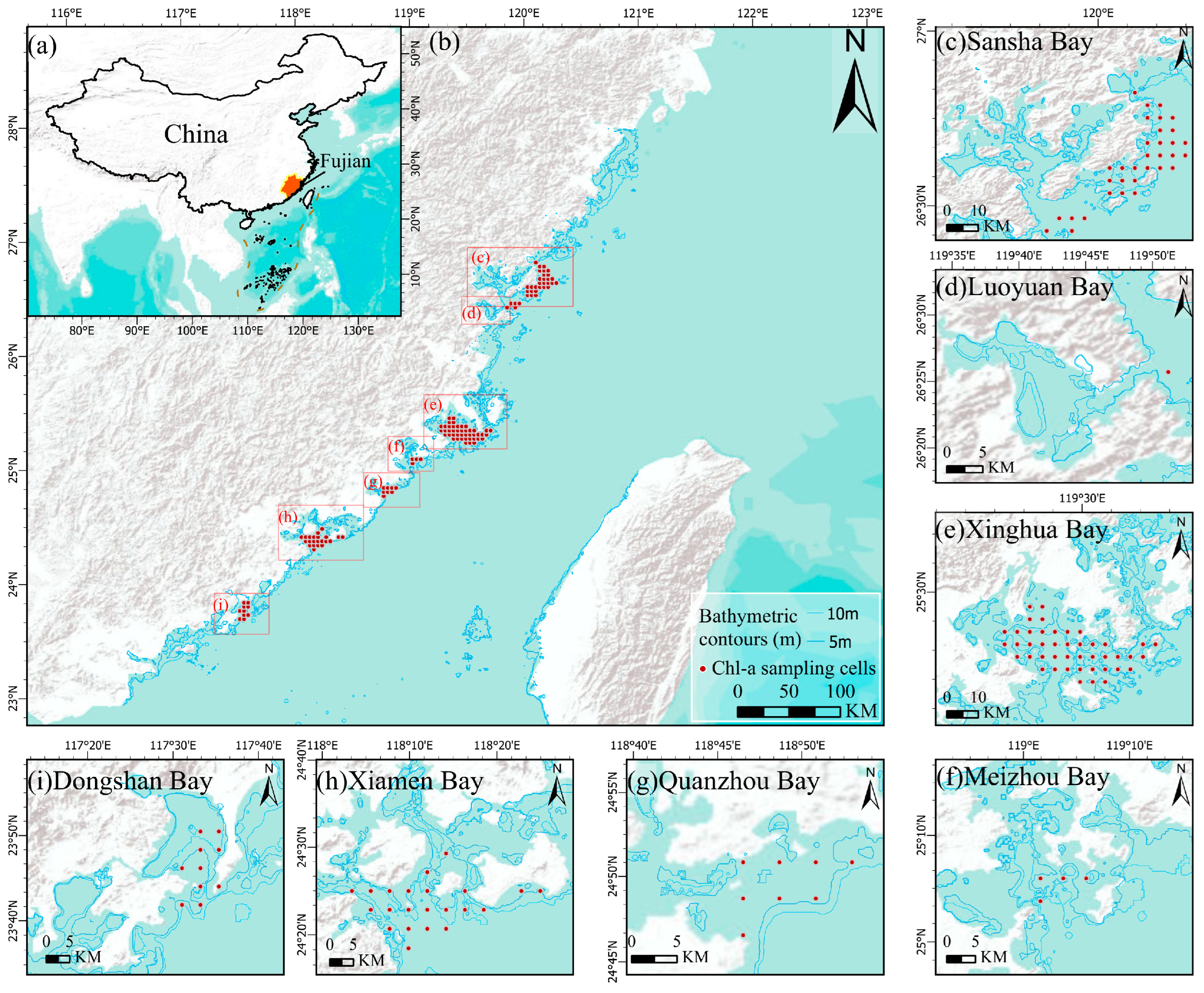
This study focuses on seven representative coastal bays in Fujian Province, southeastern China (Figure 1): Xinghua Bay (XHB), Sansha Bay (SSB), Xiamen Bay (XMB), Dongshan Bay (DSB), Quanzhou Bay (QZB), Meizhou Bay (MZB), and Luoyuan Bay (LYB). These bays are located along the western coast of the Taiwan Strait and differ in shoreline configuration, bay openness, water-exchange conditions, and coastal-use intensity. They are jointly influenced by monsoon forcing, regional circulation, riverine inputs, aquaculture activities, coastal development, and land–sea interactions. These contrasts (Table 1 and Table 2) make Fujian coastal bays suitable for examining spatial differences in long-term satellite-derived Chl-a seasonality and recurrent high-Chl-a signals.
Together, these bays represent ecologically and economically important coastal systems that support substantial mariculture and fisheries while being exposed to contrasting hydrodynamic and anthropogenic pressures. These characteristics make them suitable for examining bay-specific differences in long-term satellite-derived Chl-a seasonality and recurrent high-Chl-a exceedances.

2.2. Data Sources and Preprocessing

Satellite-derived Chl-a concentration was obtained from the Copernicus Marine satellite ocean-colour product available in Google Earth Engine (GEE), using the image collection COPERNICUS/MARINE/SATELLITE_OCEAN_COLOR/V6 and the chlor_a band. The analysis covered January 2003 to December 2024. This record was used to characterize monthly climatology, seasonal behaviour, high-anomaly frequency, and monitoring-priority patterns.
Auxiliary environmental variables included sea surface temperature (SST), precipitation, air temperature, bay-level geographic attributes, and coastal-development proxies. SST was derived from NOAA OISST V2.1, and monthly precipitation was obtained from GPM IMERG Monthly V07. Air temperature was extracted from ERA5 reanalysis and aggregated to the monthly scale; the ERA5 Daily product in GEE was used for 2003–2019, whereas the ERA5 Hourly product was aggregated to monthly means for 2020–2024. Coastal-development proxies were derived from the GHSL built-surface product, including the built-up proportion within a 10 km buffer around each sampling unit in 2000 and 2015, as well as the corresponding change. Spatial attributes included bay area and the distance from each sampling unit to the associated bay-mouth point. These variables were used to examine spatial associations with high-Chl-a anomalies and to support exploratory machine-learning diagnostics.
Detailed information on the temporal and spatial resolutions and analytical treatment of the response and predictor variables is provided in Table S1. SST, precipitation, air temperature, and wind were treated as dynamic variables and aggregated to the monthly scale, whereas stable-water fraction, built-up indicators, bay area, and distance to the bay mouth were treated as static attributes. Raster variables were linked to the approximately 4 km Chl-a sampling units without altering the native spatial information content of the source products.
Sampling units were constructed to match the nominal spacing of approximately 4 km to match the spatial resolution of the ocean-colour product. Candidate points were generated at approximately 4 km intervals within the polygons of each study bay. For each candidate point, the long-term Chl-a baseline was calculated as the geometric mean of all positive and non-missing satellite-derived Chl-a retrievals available during the study period. Long-term data availability at each point was quantified as the total number of days with an available, unmasked satellite-derived Chl-a retrieval. Candidate points with fewer than 300 satellite-retrieval days were excluded to ensure adequate long-term data support. A stable-water mask was constructed using Sentinel-2 surface-reflectance imagery acquired from 2017 to 2020. After cloud and invalid-pixel masking, the temporal median of the modified normalized difference water index (MNDWI) was calculated as follows:
MNDWI = B 3     B 11 B 3   +   B 11
where B3 is the green band and B11 is the shortwave infrared band. Pixels with median MNDWI values greater than −0.05 were classified as stable water. This water mask was then used to screen the sampling units.
Before formal analysis, the dataset was checked for date fields, sampling-unit identifiers, coordinates, duplicate records, missing values, and invalid Chl-a values. The final dataset contained 122 sampling units: 44 in Xinghua Bay, 33 in Sansha Bay, 22 in Xiamen Bay, 10 in Dongshan Bay, 8 in Quanzhou Bay, 4 in Meizhou Bay, and 1 in Luoyuan Bay. Each sampling unit was assigned a unique identifier and linked to static attributes, including bay code, bay name, coordinates, long-term Chl-a baseline, total number of valid Chl-a observations, water fraction, bay area, distance to the bay mouth, and built-up indicators.

2.3. Monthly Chl-a Aggregation and Data Reliability

Monthly Chl-a values were aggregated at the sampling-unit scale using the geometric mean to reduce the influence of episodic high values in the right-skewed Chl-a distribution [28]. For each calendar month, all valid positive Chl-a retrievals were first extracted from the Copernicus Marine ocean-colour image collection and log-transformed. The monthly mean of log-transformed Chl-a was then back-transformed to the original scale using the exponential function:
C m = e x p 1 n m i   =   1 n m ln C i
where Cm denotes the monthly geometric-mean Chl-a for a given sampling unit, Ci denotes a valid positive Chl-a observation within the month, and nm denotes the number of valid Chl-a observation days in that month.
Monthly records with nm ≥ 3 were retained. This screening yielded 19,003 valid cell-month records, with a median of 6 valid observation days per month and an interquartile range of 4–9 days. A stricter threshold of (nm ≥ 5) retained 13,340 records and was used for sensitivity analysis [17].
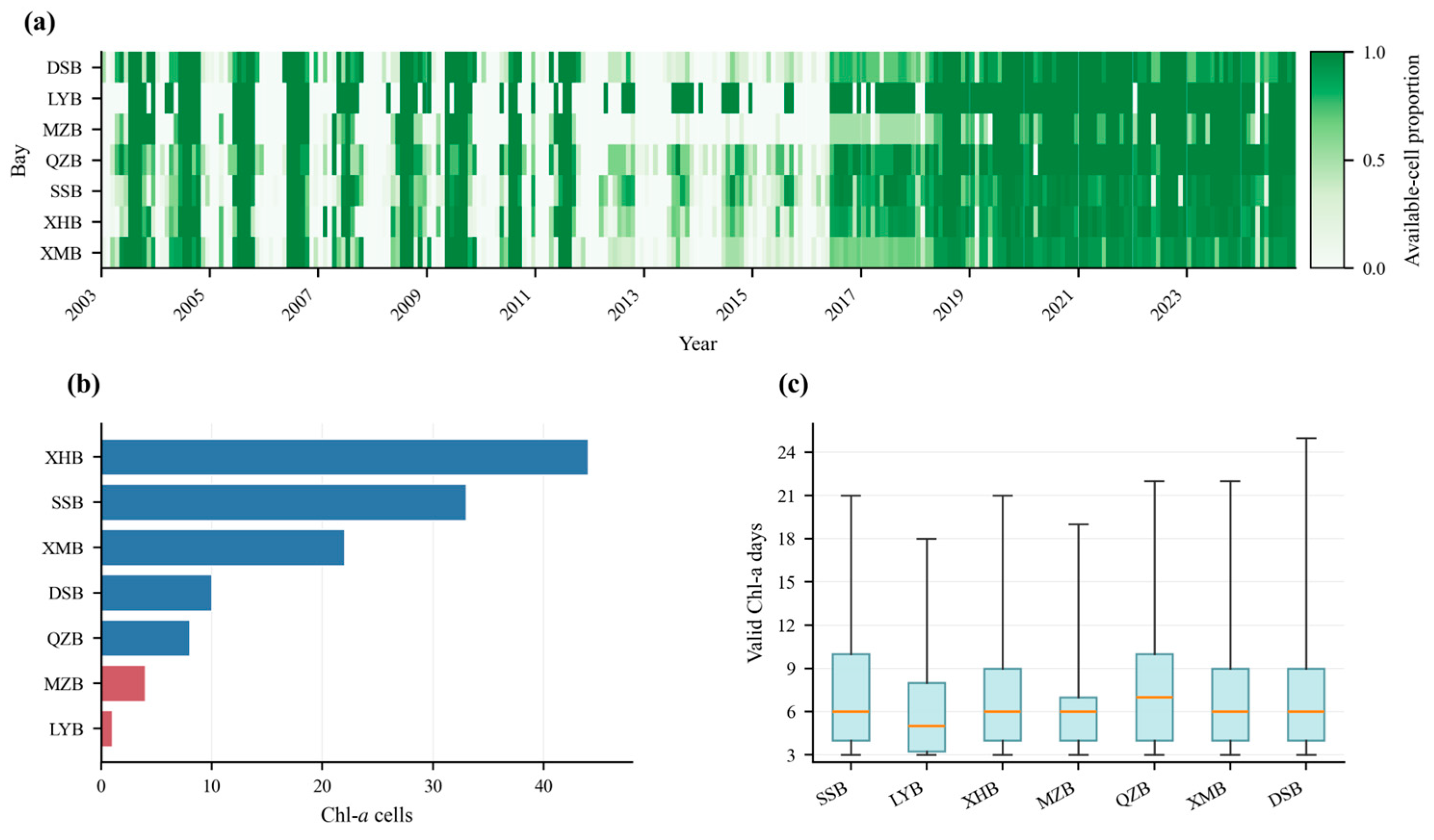
The final dataset showed uneven sampling support among bays. Xinghua Bay, Sansha Bay, and Xiamen Bay contributed most sampling units, whereas Meizhou Bay and Luoyuan Bay had limited spatial sampling support (Figure 2b). For the retained monthly records, valid Chl-a observation days generally supported the analysis, although data availability still varied among years and bays (Figure 2a,c). These differences were considered when interpreting climatological patterns and monitoring-priority areas.

2.4. Seasonal Rhythm Metrics and Type Classification

Seasonal phenological metrics were calculated from the long-term monthly climatology of each sampling unit. The main metrics included long-term geometric-mean Chl-a, monthly climatological Chl-a, seasonal amplitude, coefficient of variation, peak month, and circular peak timing [15,29]. The main metrics included the long-term geometric-mean Chl-a, monthly climatological Chl-a, seasonal amplitude, coefficient of variation (CV), peak month, and circular peak timing [30]. Seasonal amplitude was defined as the difference between the maximum and minimum monthly climatological Chl-a values:
A = C m a x C m i n
where A is the seasonal amplitude, and Cmax and Cmin are the minimum monthly climatological Chl-a values, respectively. The CV was calculated as the standard deviation of monthly climatological Chl-a divided by its mean:
C V = σ C μ C  
where σC and μC denote the standard deviation and mean of monthly climatological Chl-a, respectively. Circular peak timing was used to preserve the temporal continuity between December and January.
Exploratory seasonal phenological regimes were identified using sampling-unit-level phenological metrics. Candidate clustering methods included K-means clustering and Gaussian mixture models (GMMs), with candidate cluster numbers ranging from 2 to 6 [16,31]. All metrics were z-score-standardized before clustering. The final classification scheme was selected by jointly considering the silhouette coefficient, minimum cluster size, and ecological interpretability [32]. The main analysis adopted a four-cluster K-means solution, which grouped the sampling units into four seasonal phenological regimes, denoted as C0–C3.
Throughout this study, “seasonal Chl-a dynamics” refers to the observed intra-annual variation in Chl-a, whereas “seasonal phenological regimes” refers specifically to the four cluster-derived classes (C0–C3).

2.5. Monitoring-Priority Classification

High-Chl-a anomalies were defined using percentile thresholds to account for background differences among sampling units, bays, and calendar months. Three P90-based anomaly definitions were compared [18,33].
The first definition was the cell-month P90 threshold, calculated separately for each sampling unit and calendar month. A monthly geometric-mean Chl-a record was labelled as a high anomaly when it exceeded the historical 90th percentile for the same sampling unit and calendar month.
The second definition was the bay-month P90 threshold, calculated from all valid monthly cell records within the same bay and calendar month. A sampling-unit record was classified as a high anomaly when its monthly Chl-a exceeded the corresponding bay-month threshold. This definition preserved the calendar-month background within each bay while retaining spatial contrasts among sampling units in the same bay. Therefore, it was adopted as the primary definition for monitoring-priority classification.
The third definition was the regional-month P90 threshold, calculated from all valid records across the seven bays for the same calendar month. This definition was used as a comparative benchmark to evaluate how regional-scale normalization affected anomaly frequency and hotspot patterns.
For each definition, the high-anomaly frequency of each sampling unit was calculated as the proportion of valid monthly records classified as high anomalies. These frequencies were used to compare anomaly definitions, map recurrent high-Chl-a areas, and support monitoring-priority classification.
Sampling units with high anomaly frequency and sufficient data support were assigned to higher monitoring priority. Units with moderate anomaly frequency or intermediate data support were assigned to medium priority. Units with low anomaly frequency were assigned to lower priority. Sampling units with limited data support were flagged for cautious interpretation, even when their anomaly frequency was high. This rule reduced the influence of sparse observations on the final priority map and aligned the classification with the data-reliability constraints of the satellite record.

2.6. Machine-Learning Assessment

A machine-learning assessment was conducted to examine whether hydrometeorological, geographic, and coastal-development proxy variables contained information related to the susceptibility of high-Chl-a anomalies. This assessment served as a diagnostic component of the monitoring framework and was interpreted through model performance under multiple validation schemes.
Two modelling tasks were defined. For the classification task, the binary occurrence of high anomalies under the primary bay-month P90 definition was used as the response variable. For the regression task, the standardized Chl-a anomaly was used as a continuous response variable. Candidate predictors included sea surface temperature, air temperature, precipitation, 10 m wind components, wind speed, distance to the bay mouth, bay area, stable-water fraction, built-up proportion, built-up growth, month, and year. Sampling-unit identifier, bay code, bay name, longitude, and latitude were excluded from the predictor set to reduce direct spatial memorization.
Three algorithm groups were compared. Logistic regression was used as the linear baseline for the classification task, with continuous predictors standardized before model fitting. Random forest was used as a nonlinear ensemble model [34]. It predicts by fitting multiple decision trees on bootstrap samples and random predictor subsets, allowing nonlinear associations and interactions among predictors to be represented. Histogram-based gradient boosting was used as a boosting model [35]. It improves predictive performance by sequentially updating decision-tree learners and is computationally efficient for tabular data. Corresponding regression variants were used for the continuous-anomaly prediction task where applicable.
Model performance was evaluated using three validation schemes: random train–test splitting, bay-grouped validation, and temporal holdout validation using 2020–2024 as the test period [36]. Classification performance was assessed using ROC-AUC, PR-AUC, and calibration behaviour [37,38]. Regression performance was assessed using RMSE and MAE. Permutation importance was calculated on validation data to summarize predictor contributions [39]. The machine-learning results were interpreted as exploratory susceptibility diagnostics within the broader Chl-a monitoring framework.

3. Results

3.1. Monthly Chl-a Seasonal Dynamics Among Bays

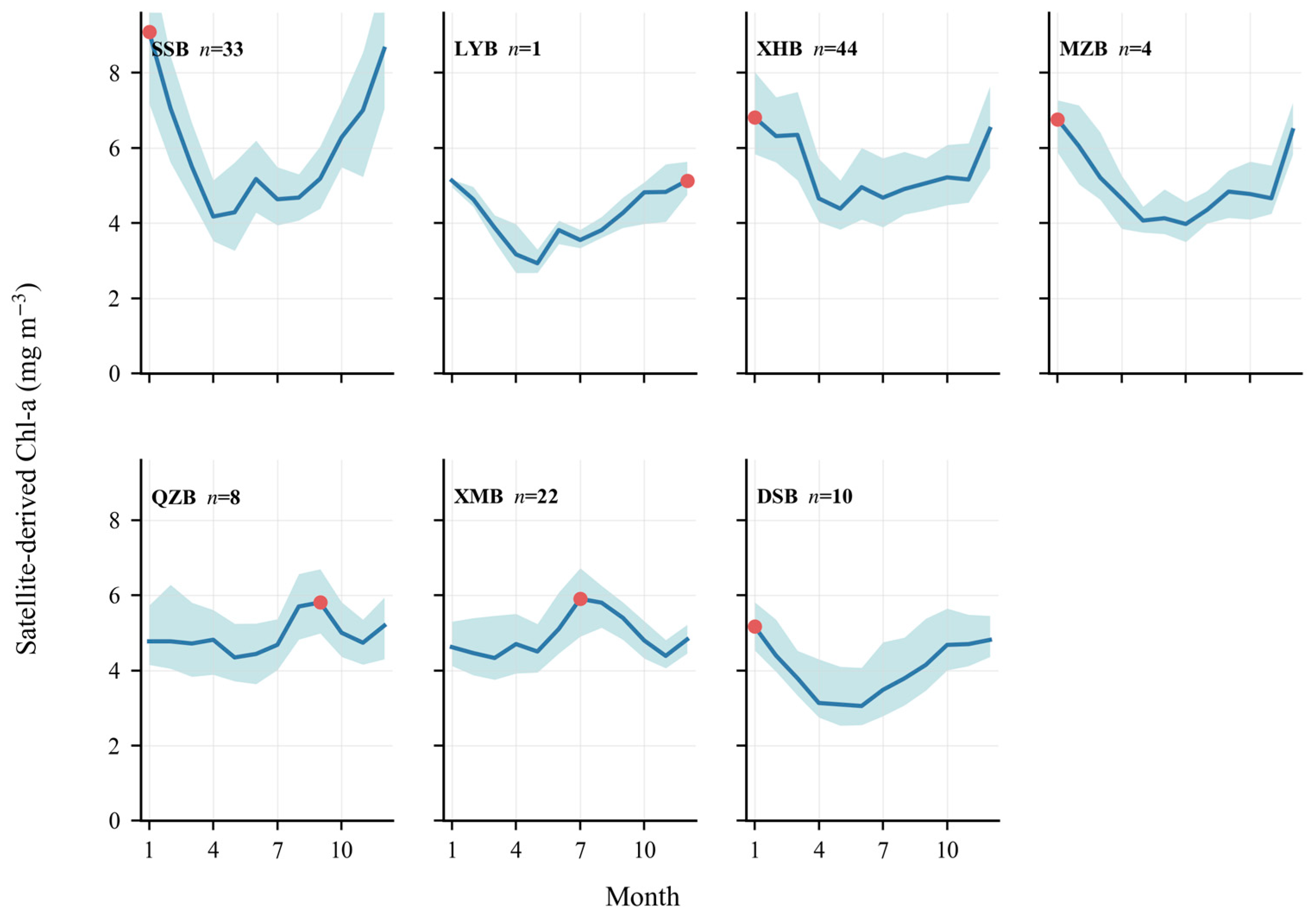
Bay-scale monthly climatology shows clear seasonal differences in satellite-derived Chl-a among the seven Fujian coastal bays (Figure 3). Several bays exhibit elevated Chl-a during winter, although peak timing and seasonal amplitude vary among bays. Sansha Bay (SSB) shows the strongest seasonal contrast, with winter maxima (4.92 mg m−3, Dec–Jan) and a pronounced spring minimum (4.18 mg m−3, Apr–May). Xinghua Bay (XHB) displays a similar winter-enhanced pattern, characterized by high winter values, a decline during spring, and a gradual increase toward late autumn and winter. Dongshan Bay (DSB) and Meizhou Bay (MZB) also show higher Chl-a in winter. In contrast, Xiamen Bay (XMB) exhibits its maximum in summer (Jul), with median Chl-a reaching its maximum around July. Quanzhou Bay (QZB) has the smallest peak-to-trough range among the seven bays (1.46 mg m−3), with monthly median Chl-a ranging from 4.35 mg m−3 in May to 5.81 mg m−3 in September.
Overall, the monthly climatology reveals a broadly shared regional pattern, with winter Chl-a maxima and spring-to-early-summer minima in most of the surveyed bays. However, the timing and magnitude of seasonal variation differ among bays, with Xiamen Bay (XMB) and Quanzhou Bay (QZB) showing the clearest departures from this general pattern. Xiamen Bay reaches its maximum median Chl-a in summer (Jul), whereas Quanzhou Bay exhibits a comparatively flatter seasonal trajectory and reaches its maximum in autumn (Sep). These shared and contrasting bay-scale patterns were further examined at the sampling-unit scale through the classification of seasonal phenological regimes and the screening of recurrent high-Chl-a exceedances.

3.2. Spatial Distribution of Seasonal Chl-a Phenological Regimes

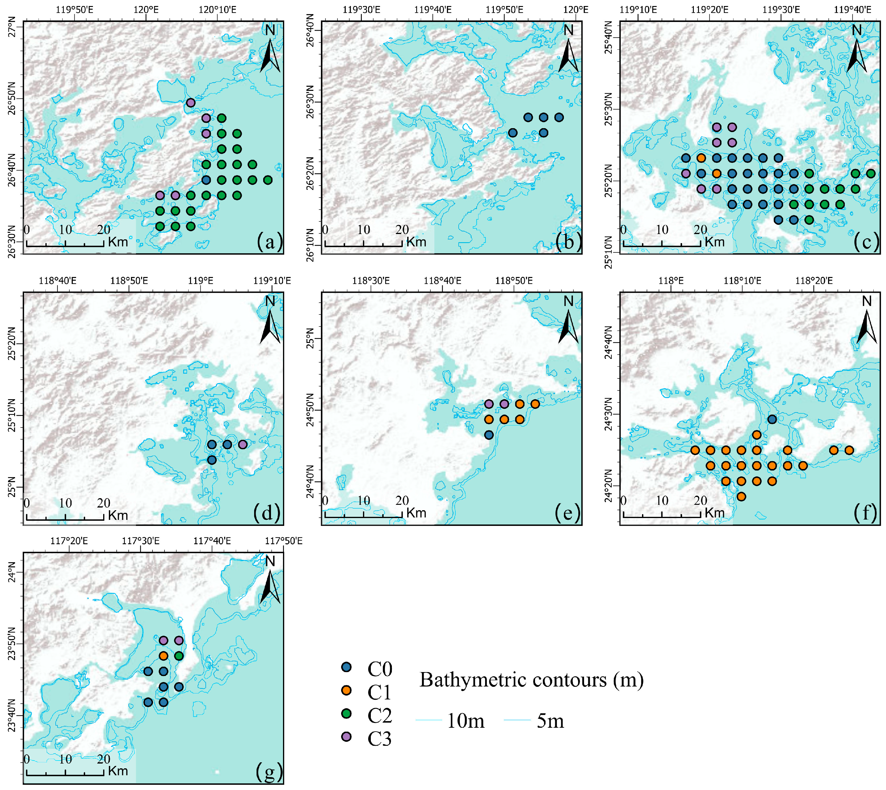
The exploratory seasonal Chl-a phenological regimes show pronounced spatial heterogeneity among and within Fujian coastal bays (Figure 4). Some bays are characterized mainly by one or twophenological regimes, whereas multiple regimes coexistwithin Sansha and Xinghua Bays. These results indicate that the seasonality of satellite-derived Chl-a is spatially structured at both the bay scale and the intra-bay scale.
Sansha Bay (SSB) and Xinghua Bay (XHB) show the strongest intra-bay heterogeneity. In Sansha Bay, C2 occupies a large proportion of the retained sampling units, whereas C0 and C3 also occur in several local areas, indicating distinct seasonal Chl-a phenological regimes within the same bay. Xinghua Bay likewise contains all four types, C0–C3, with different regime distributed between inner-bay settings and relatively open-water sampling units. These two bays therefore show the clearest co-occurrence of multiple seasonal Chl-a behaviours within a single bay.
The spatial composition of the other bays is relatively simpler. Xiamen Bay (XMB) is dominated by C1, with only a few sampling units assigned to other rhythm types, indicating a comparatively consistent seasonal Chl-a pattern. Quanzhou Bay (QZB) contains fewer retained sampling units and is composed mainly of C0 and C1. Dongshan Bay (DSB) also shows a relatively simple type composition, although local differences among C0, C1, and C3 are still present. Luoyuan Bay (LYB) and Meizhou Bay (MZB) retain only a small number of sampling units and therefore mainly provide local-scale rhythm information.

3.3. Seasonal Characteristics of the Four Phenological Regimesa

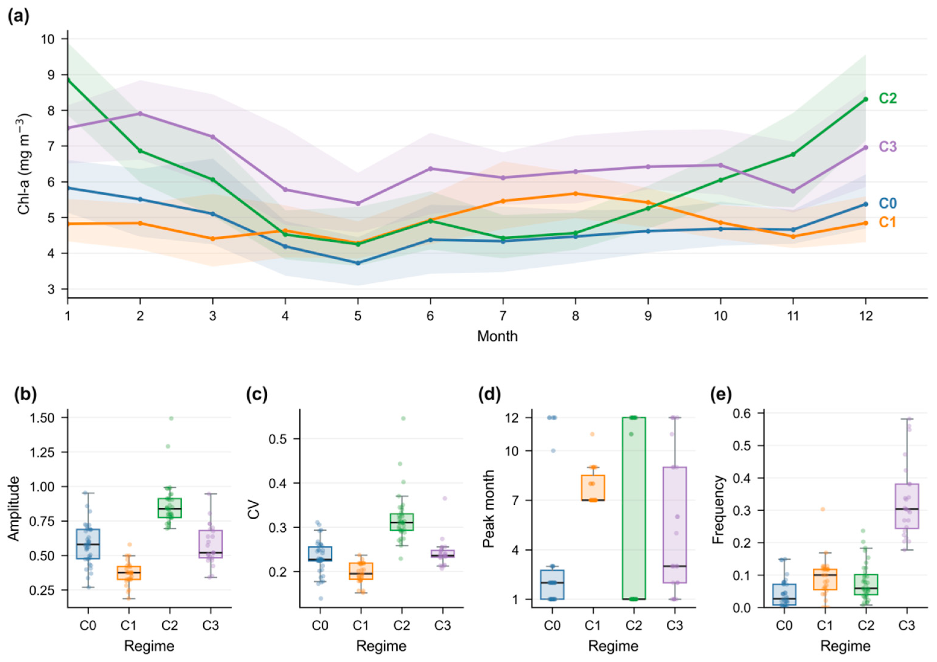
The four seasonal phenological regimes show systematic differences in monthly Chl-a trajectories and phenological metrics (Figure 5). C0 represents an intermediate seasonal pattern. Chl-a remains within a moderate range in most months, and its seasonal amplitude and variability metrics are also intermediate among the four types. C1 is the most stable seasonal type. Its monthly curve is relatively flat, and both seasonal amplitude and coefficient of variation (CV) are lower than those of the other types. This combination indicates that C1 represents a low-amplitude Chl-a seasonal regime.
C2 shows the strongest seasonal contrast. Its Chl-a curve declines from relatively high winter values to a spring minimum and then increases again toward the late-year months. This trajectory is consistent with the metric distributions: C2 has the highest seasonal amplitude and the highest CV. The agreement between curve shape and metric summaries indicates that C2 represents a winter-enhanced, high-amplitude seasonal regime. C3 shows a different feature. Its Chl-a remains relatively high across multiple months, and its high-anomaly frequency is the highest among the four types. This pattern indicates that C3 is characterized by frequent exceedance of its background threshold rather than by a single seasonal pulse. In this sense, C3 represents a high-anomaly-prone Chl-a seasonal regime, whereas C2 represents a high-amplitude seasonal Chl-a rhythm type.
Taken together, Figure 4 and Figure 5 show that Chl-a variability in representative Fujian coastal bays is expressed through three related dimensions: spatial location, seasonal curve shape, and anomaly tendency. The rhythm-type classification integrates these dimensions into a sampling-unit-scale analytical framework. The results indicate that water units with different seasonal Chl-a dynamics can coexist within the same bay. Differences among rhythm types were reflected not only in mean concentration levels, but also in seasonal amplitude, relative variability, peak timing, and high-Chl-a anomaly frequency.

3.4. Monitoring-Priority Zones Based on Chl-a Phenology and High-Anomaly Frequency

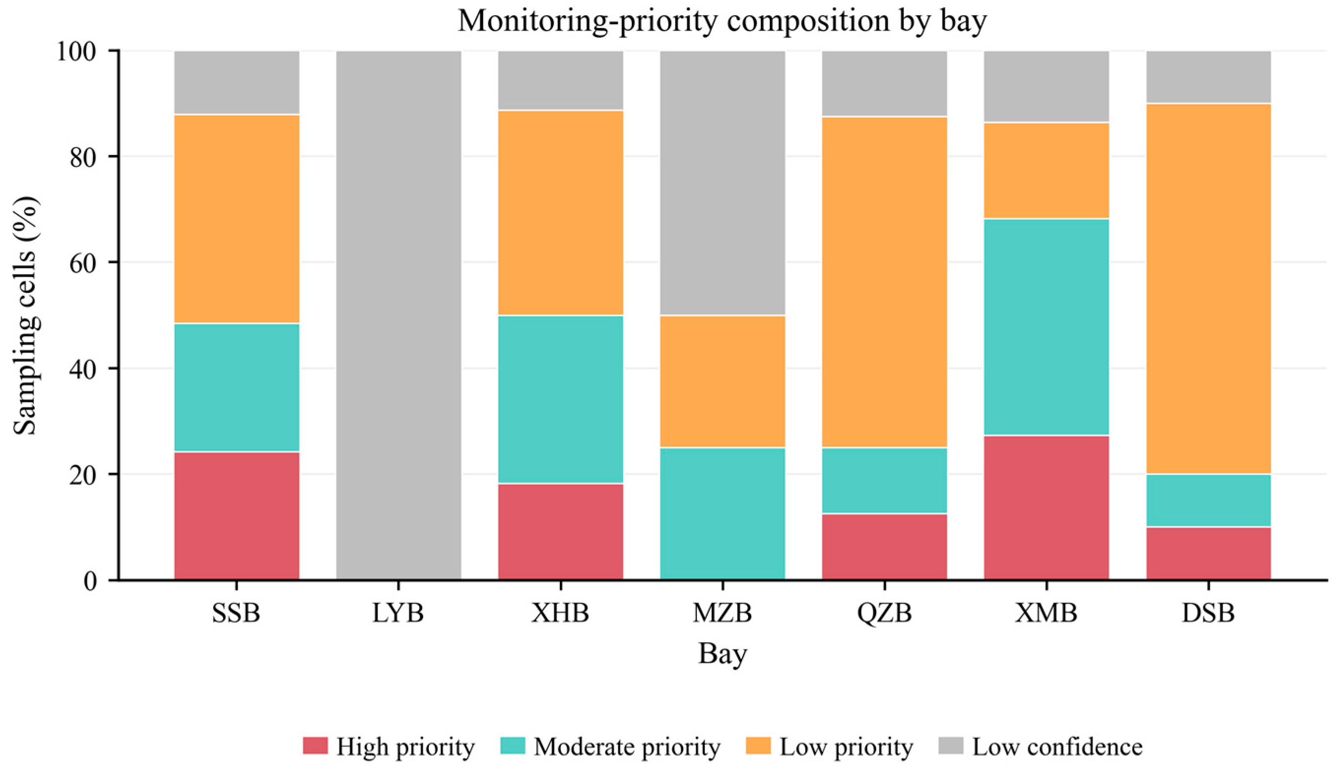
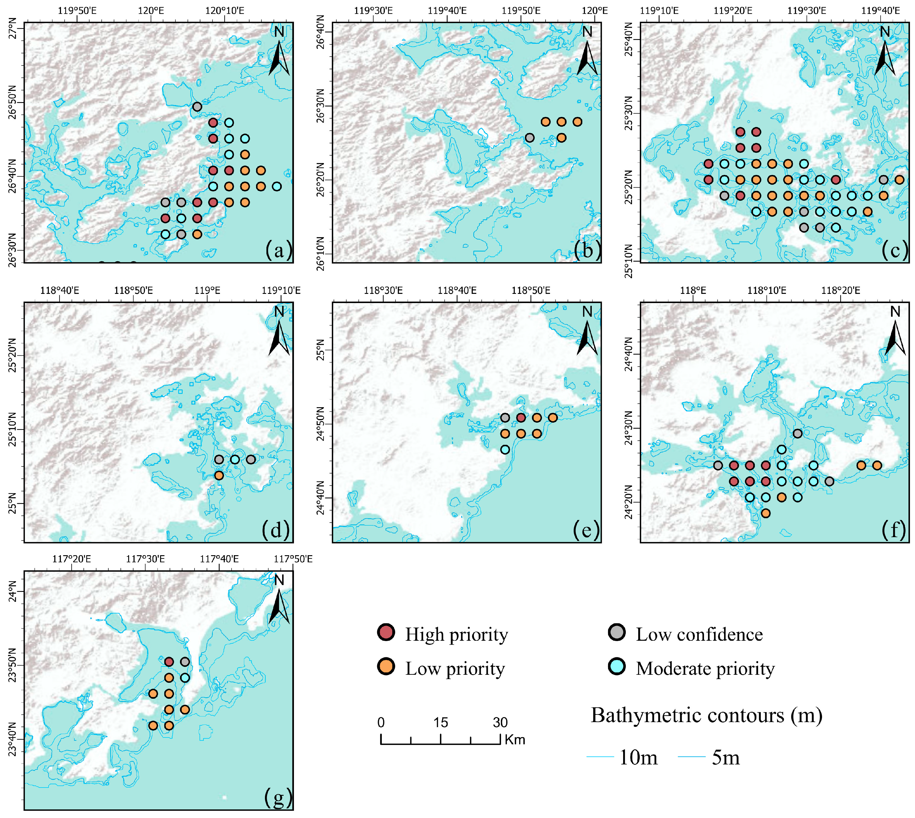
The monitoring-priority classification translates sampling-unit-scale Chl-a phenological characteristics and high-anomaly information into a spatial screening layer for bay monitoring (Figure 6 and Figure 7). The resulting priority classes are unevenly distributed both among bays and within individual bays. High-priority and medium-priority units are most evident in Sansha Bay (SSB), Xinghua Bay (XHB), and Xiamen Bay (XMB), whereas Quanzhou Bay (QZB) and Dongshan Bay (DSB) are dominated mainly by low-priority units, with only a few localized high- or medium-priority units.
SSB and XHB show the clearest intra-bay heterogeneity. In both bays, high-priority, medium-priority, low-priority, and low-confidence units occur simultaneously, indicating that monitoring concern varies substantially at the intra-bay scale. In SSB, high- and medium-priority units are interspersed with low-priority units across the retained sampling grid. XHB shows a similar mixed pattern, in which high- and medium-priority units co-occur with extensive low-priority areas. These results indicate that bay-scale summary values alone would obscure localized monitoring-priority zones.
Overall, the monitoring-priority classification indicates that recurrent high-Chl-a signals and pronounced phenological variability are not evenly distributed along the Fujian coast. SSB, XHB, and XMB contain the main concentrations of high- and medium-priority units, whereas QZB and DSB show more localized priority patterns. Luoyuan Bay (LYB) and Meizhou Bay (MZB) primarily reflect the limitation of insufficient data support. This screening result provides a spatial basis for subsequent field validation and targeted monitoring in coastal bays.

3.5. Exploratory Machine-Learning Diagnostics of High-Chl-a Anomaly Susceptibility

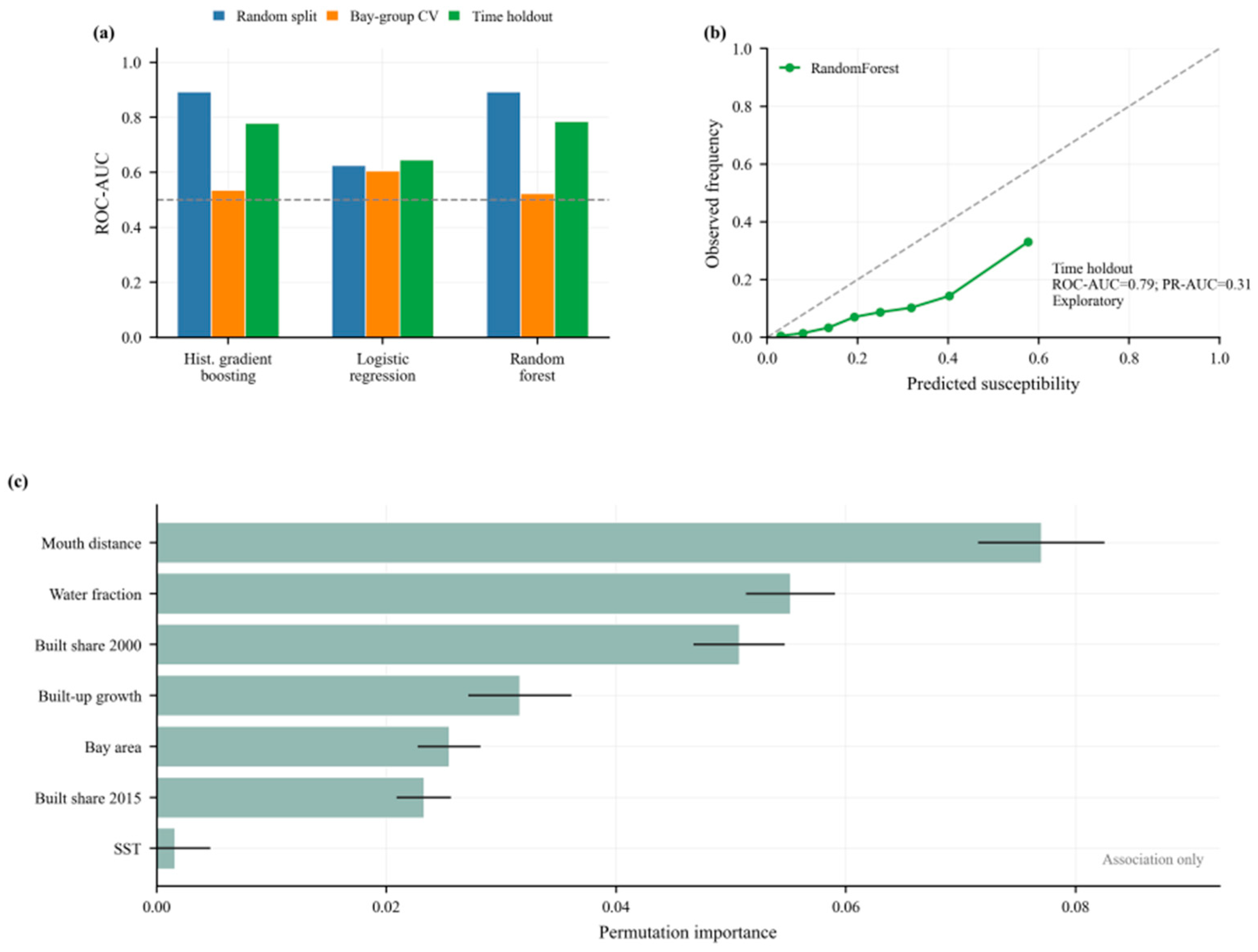
Exploratory machine-learning assessment indicates that the susceptibility of high-Chl-a anomalies contains diagnostic information, but model performance is sensitive to the validation strategy (Figure 8). Under random splitting, the histogram-based gradient boosting model and random forest achieve relatively high ROC-AUC values. Under bay-group cross-validation, however, tree-based models show a marked performance decline, indicating limited transferability across bays. In the temporal holdout validation, the random forest retain moderate discriminatory ability, with a ROC-AUC of approximately 0.79. The calibration curve showed that observed high-anomaly frequency generally increases with predicted susceptibility, although the calibration points remain below the ideal 1:1 line. This suggests that the model is more suitable for relative susceptibility ranking than for calibrated probability estimation. Permutation importance shows that distance to bay mouth, stable-water fraction, and built-surface percentage in 2000 are the leading contributors, indicating that spatial setting, water-pixel dominance, and coastal-development background contain exploratory diagnostic information related to recurrent high-Chl-a signals.

4. Discussion

4.1. Main Spatiotemporal Patterns of Chl-a in Fujian Coastal Bays

The monthly climatology shows that satellite-derived Chl-a seasonality in Fujian coastal bays cannot be reduced to a single regional pattern (Figure 3). Sansha Bay and Xinghua Bay exhibited strong winter or late-year Chl-a signals, Xiamen Bay showed a warm-season peak, and Quanzhou Bay displayed weaker seasonality with a moderate increase in early autumn. These contrasts indicate that annual mean Chl-a or bay-scale averages may obscure key seasonal information, including peak timing, seasonal amplitude, and intra-annual trajectories. This interpretation is consistent with recent phytoplankton phenology research showing that bloom peak timing, maximum concentration, amplitude, and duration provide ecological information that cannot be captured by mean biomass alone [29].
These seasonal differences should be interpreted within the regional hydroclimatic setting of the western Taiwan Strait. Monsoon forcing, strait circulation, coastal currents, plume transport, wind mixing, and stratification can modify light availability, nutrient supply, water residence time, and water-mass exchange [20,40,41,42]. Recent work in the Taiwan Strait further indicates that phytoplankton responses to plume influence and nutrient limitation can be nonlinear, with Chl-a not necessarily increasing in proportion to river-derived material inputs [43]. This regional complexity provides a plausible background for the coexistence of winter-enhanced, warm-season, and weakly seasonal Chl-a patterns along the Fujian coast.
At the bay scale, local geomorphology and land–sea interactions may further modulate this regional seasonal forcing. Semi-enclosed bays differ in openness, water-exchange efficiency, shoreline complexity, aquaculture intensity, and proximity to riverine or urban inputs. These factors can affect turbidity, nutrient retention, water residence time, and the coupling between inner-bay and offshore waters. Similar bay-scale modulation has been reported in Zhanjiang Bay, where seasonal and spatial Chl-a patterns were attributed to the combined influence of land-derived nutrient transport, aquaculture activities, climatic conditions, hydrodynamic processes, and adjacent coastal currents [13]. The Fujian results therefore indicate that comparable regional forcing can generate distinct Chl-a seasonal trajectories after being filtered by local bay morphology and water-exchange conditions.

4.2. Phenological Regimes and Within-Bay Heterogeneity

The seasonal phenological regimes identified in Figure 4 and Figure 5 show that Chl-a variability in Fujian coastal bays cannot be adequately described by mean concentration alone. Instead, differences among sampling units were expressed through seasonal amplitude, peak timing, intra-annual trajectory, and exceedance recurrence. This multidimensional interpretation is consistent with satellite-based phenology studies showing that peak timing, intensity, duration, and recurrence provide ecological information that is not captured by mean Chl-a alone [29,44,45].
The coexistence of multiple seasonal phenological regimes within Sansha Bay and Xinghua Bay is particularly important because it demonstrates that bay-scale climatological averages can mask substantial intra-bay heterogeneity. Sampling units located in inner-bay waters, tidal channels, bay-mouth areas, and relatively open waters may experience different combinations of material retention, tidal exchange, riverine influence, turbidity, and seasonal mixing, thereby producing distinct seasonal Chl-a trajectories within the same semi-enclosed system. Comparable intra-bay differentiation has been reported in coastal and semi-enclosed systems, where phytoplankton-related Chl-a patterns are jointly influenced by nutrient availability, plume transport, water exchange, hydrodynamic processes, and local environmental gradients [13,43,46]. For Sansha Bay, previous studies have also shown that intensive mariculture, riverine inputs, and complex hydrodynamic processes can affect nutrient budgets and biogeochemical variability, providing a plausible context for the observed coexistence of multiple phenological regimes [25,47]. Consequently, sampling units exposed to similar regional monsoon forcing may still exhibit different seasonal trajectories because local hydrogeomorphic conditions modify the regional signal. From a monitoring perspective, this finding indicates that bay-wide averages alone may overlook localized water bodies with distinct phenological behaviour or recurrent high-Chl-a exceedances.
The contrast between C2 and C3 further illustrates why seasonal amplitude and exceedance recurrence should be interpreted separately in monitoring applications. A high-amplitude seasonal cycle, as represented by C2, reflects predictable intra-annual variation, whereas the recurrent exceedances associated with C3 indicate repeated departures from the bay- and month-specific background. Thus, a sampling unit with pronounced seasonality does not necessarily represent a location with recurrent monitoring concern. For Fujian coastal bays, separating these two dimensions prevents predictable seasonal maxima from being treated as equivalent to recurrent high-Chl-a exceedance and provides a clearer basis for monitoring-priority screening.

4.3. Monitoring-Priority Differentiation and Exploratory Environmental Diagnostics

The monitoring-priority structure differed markedly among bays (Figure 6 and Figure 7). Sansha Bay (SSB) and Xinghua Bay (XHB) contained more high-priority and medium-priority units, and multiple priority classes coexisted within each bay (Figure 7). This spatial heterogeneity was consistent with the seasonal phenological-regime analysis, which identified multiple seasonal Chl-a regimes within the larger bays. These large and geomorphologically complex bays share several conditions that may favour the accumulation, persistence, and recurrence of high-Chl-a states: restricted inner-bay water exchange, land-derived nutrient inputs from river discharge and urban runoff, and intensive coastal aquaculture. In Fujian nearshore waters, high-Chl-a signals have been reported around major mariculture bays, including SSB and XHB. In SSB, nutrient dynamics are influenced jointly by riverine inputs, intensive mariculture, and exchange with adjacent coastal water [47,48,49]. A historical source assessment across seven Fujian bays reported the highest total nitrogen and total phosphorus loads in XHB and identified land-based discharges and aquaculture as major regional pollution sources [26]. Published studies also document substantial anthropogenic nutrient pressures in XMB and QZB, although the main source areas differ: major pollution inputs to XMB are concentrated around the Jiulong River Estuary and the western and northern inner-bay waters, whereas higher nutrient pressure in QZB occurs near the Jinjiang Estuary, the southern inner bay, and shoreline outfalls. The higher-priority units were mainly located in inner-bay settings, where nutrients delivered by river discharge and urban runoff, together with aquaculture-derived materials, may be retained for longer periods under limited flushing conditions. Bay-mouth and relatively open-water units are more strongly affected by tidal flushing, dilution, and offshore exchange, which may reduce the persistence of locally elevated Chl-a. This spatial pattern indicates that recurrent high-Chl-a signals are structured by both bay-scale contrasts and intra-bay gradients.
Monsoon alternation provides a temporal gating mechanism through which these spatial gradients are expressed as phenological signals. During the northeast monsoon season, enhanced coastal currents, vertical mixing, and nearshore water intrusion can replenish nutrients in semi-enclosed bays and sustain elevated winter–spring Chl-a conditions (Figure 3).
During the southwest monsoon season, wind-driven upwelling along the western Taiwan Strait and in topographically favourable areas may inject subsurface nutrients into the euphotic zone and modify the timing of summer Chl-a enhancement [50]. These seasonal source pathways provide bay-specific context for the observed Chl-a patterns. In SSB, winter nutrient enrichment has been linked to the intrusion of nutrient-rich coastal water superimposed on mariculture inputs, whereas XMB experiences strong flood-season pollutant delivery through the Jiulong River and a documented concentration of historical red-tide events in late spring and summer [47,51,52]. Ecological responses within Fujian bays depend on whether these external nutrient pulses are retained long enough to support phytoplankton growth. The same upwelling signal may generate a clear Chl-a response in retention-prone inner-bay waters, appear weaker near well-flushed bay mouths, or form transient offshore high-Chl-a patches when biomass is mainly controlled by lateral transport [53].
Distance to the bay mouth provides an integrated spatial proxy for this inner-bay–bay-mouth gradient. This variable primarily represents differences in water-exchange intensity, tidal flushing, residence time, dilution capacity, and material-retention potential. River discharge, urban runoff, sewage outfalls, and many aquaculture activities are commonly concentrated near river estuaries, shorelines, and inner-bay waters, whereas coastal-current intrusion and upwelling may deliver nutrients from the bay mouth or adjacent shelf. It therefore helps explain why recurrent high-Chl-a anomalies were more likely to occur in exchange-limited inner-bay units. In the machine-learning diagnostics, distance to the bay mouth ranked highest in random forest permutation importance (Figure 8c), further supporting the inference that high-anomaly susceptibility is strongly constrained by the intra-bay exchange–residence–dilution continuum. This result is consistent with the inward concentration of high-priority units shown in Figure 6 and Figure 7.

4.4. Uncertainty Analysis and Limitations

Several sources of uncertainty define the spatial and interpretive scope of this satellite-based screening framework. Satellite-derived Chl-a in coastal waters can be affected by optical complexity, suspended particulate matter, coloured dissolved organic matter, shallow-water effects, and algorithm uncertainty [54,55,56]. In addition, the approximately 4 km sampling-unit scale cannot resolve fine-scale aquaculture structures, small estuarine plumes, or nearshore gradients. Only one and four retained satellite-based sampling units were available for Luoyuan Bay and Meizhou Bay, respectively. Their results therefore provide localized descriptive evidence rather than bay-representative estimates. These bays were retained to preserve regional geographic coverage and to demonstrate the application of the framework under limited spatial coverage, whereas the principal comparative interpretations were based on the five bays with broader retained-unit representation. Targeted field validation would further clarify the ecological interpretation of recurrent high-Chl-a exceedances, while the present framework provides a reproducible approach for regional screening and monitoring-priority identification.

5. Conclusions

This study used a reproducible sampling-unit framework to characterize long-term satellite-derived Chl-a dynamics in seven representative Fujian coastal bays. The results showed clear differences in Chl-a seasonality among bays. Sansha Bay and Xinghua Bay exhibited strong winter or late-year signals, Xiamen Bay showed a warm-season peak, and Quanzhou Bay reached a local peak in early autumn.
At the sampling-unit scale, four seasonal phenological regimes were identified. C2 represented a winter-enhanced, high-amplitude regime, whereas C3 was associated with more frequent bay-relative high-Chl-a anomalies. The coexistence of multiple phenological types within Sansha Bay and Xinghua Bay indicates substantial intra-bay heterogeneity.
The monitoring-priority classification translated seasonal rhythm and high-anomaly information into a spatial screening layer. High-priority and medium-priority units were concentrated mainly in Sansha Bay and Xinghua Bay, whereas Dongshan Bay and Quanzhou Bay showed more localized high-priority units. The proposed workflow provides an interpretable basis for targeted coastal-bay monitoring and subsequent field validation.

Supplementary Materials

The following supporting information can be downloaded at: https://www.mdpi.com/article/10.3390/w18151917/s1. Table S1: Sources, spatial and temporal resolutions, and preprocessing procedures for the environmental variables used in the analysis.

Author Contributions

Conceptualization, D.L., B.Z., X.L. and Y.S.; methodology, B.Z. and X.L.; software, B.Z.; validation, B.Z., C.L., X.X., J.F. and G.Z.; formal analysis, B.Z.; investigation, B.Z., C.L., X.X., J.F. and G.Z.; resources, Y.S. and X.X.; data curation, B.Z.; writing—original draft preparation, B.Z.; writing—review and editing, D.L., X.L., Y.S., C.L., X.X., J.F. and G.Z.; visualization, B.Z.; supervision, Y.S. and X.X.; project administration, Y.S.; funding acquisition, Y.S. All authors have read and agreed to the published version of the manuscript.

Funding

This research was funded by the National Natural Science Foundation of China (Grant No. 42301002), and the Science & Technology Project of Water Resources Department of Fujian Province (Grant No. MSK202524).

Data Availability Statement

Datasets generated during the current study are available from the corresponding author on reasonable request.

Conflicts of Interest

The authors declare no conflicts of interest.

References

  1. Kennish, M.J. Environmental threats and environmental future of estuaries. Environ. Conserv. 2002, 29, 78–107. [Google Scholar] [CrossRef]
  2. Halpern, B.S.; Walbridge, S.; Selkoe, K.A.; Kappel, C.V.; Micheli, F.; D’Agrosa, C.; Bruno, J.F.; Casey, K.S.; Ebert, C.; Fox, H.E.; et al. A global map of human impact on marine ecosystems. Science 2008, 319, 948–952. [Google Scholar] [CrossRef] [PubMed]
  3. Yamaguchi, R.; Rodgers, K.B.; Timmermann, A.; Stein, K.; Schlunegger, S.; Bianchi, D.; Dunne, J.P.; Slater, R.D. Trophic level decoupling drives future changes in phytoplankton bloom phenology. Nat. Clim. Change 2022, 12, 469–476. [Google Scholar] [CrossRef]
  4. Powley, H.R.; Bruggeman, J.; Hopkins, J.; Smyth, T.; Blackford, J. Sensitivity of shelf sea marine ecosystems to temporal resolution of meteorological forcing. J. Geophys. Res. Ocean. 2020, 125, e2019JC015922. [Google Scholar] [CrossRef]
  5. Cloern, J.E.; Jassby, A.D. Patterns and scales of phytoplankton variability in estuarine-coastal ecosystems. Estuaries Coasts 2010, 33, 230–241. [Google Scholar] [CrossRef]
  6. Liu, X.; Laws, E.A.; Xie, Y.; Wang, L.; Lin, L.; Huang, B. Uncoupling of seasonal variations between phytoplankton chlorophyll a and production in the East China Sea. J. Geophys. Res. Biogeosci. 2019, 124, 2400–2415. [Google Scholar] [CrossRef]
  7. Behrenfeld, M.J.; O’Malley, R.T.; Siegel, D.A.; McClain, C.R.; Sarmiento, J.L.; Feldman, G.C.; Milligan, A.J.; Falkowski, P.G.; Letelier, R.M.; Boss, E.S. Climate-driven trends in contemporary ocean productivity. Nature 2006, 444, 752–755. [Google Scholar] [CrossRef] [PubMed]
  8. Siegel, D.A.; Doney, S.C.; Yoder, J.A. The North Atlantic spring phytoplankton bloom and Sverdrup’s critical depth hypothesis. Science 2002, 296, 730–733. [Google Scholar] [CrossRef] [PubMed]
  9. McClain, C.R. A decade of satellite ocean color observations. Annu. Rev. Mar. Sci. 2009, 1, 19–42. [Google Scholar] [CrossRef] [PubMed]
  10. Platt, T.; Sathyendranath, S. Ecological indicators for the pelagic zone of the ocean from remote sensing. Remote Sens. Environ. 2008, 112, 3426–3436. [Google Scholar] [CrossRef]
  11. Groom, S.; Sathyendranath, S.; Ban, Y.; Bernard, S.; Brewin, R.; Brotas, V.; Brockmann, C.; Chauhan, P.; Choi, J.; Chuprin, A.; et al. Satellite ocean colour: Current status and future perspective. Front. Mar. Sci. 2019, 6, 485. [Google Scholar] [CrossRef] [PubMed]
  12. Sathyendranath, S.; Brewin, R.J.W.; Brockmann, C.; Brotas, V.; Calton, B.; Chuprin, A.; Cipollini, P.; Couto, A.B.; Dingle, J.; Doerffer, R.; et al. An ocean-colour time series for use in climate studies: The experience of the Ocean-Colour Climate Change Initiative (OC-CCI). Sensors 2019, 19, 4285. [Google Scholar] [CrossRef] [PubMed]
  13. Wang, S.; Zhou, F.; Chen, F.; Zhu, Q.; Meng, Y. Spatial and seasonal variations of chlorophyll a in Zhanjiang Bay, China, and controlling factors. Front. Mar. Sci. 2024, 11, 1329864. [Google Scholar] [CrossRef]
  14. Zhang, J.; Zhang, Y.; Sun, X. The spatial and temporal distributions of chlorophyll-a and its relationship with main environmental factors in Zhanjiang Bay in 2009. Adv. Mar. Sci. 2012, 30, 236–243. [Google Scholar]
  15. Platt, T.; White, G.N.; Zhai, L.; Sathyendranath, S.; Roy, S. The phenology of phytoplankton blooms: Ecosystem indicators from remote sensing. Ecol. Model. 2009, 220, 3057–3069. [Google Scholar] [CrossRef]
  16. D’Ortenzio, F.; Ribera d’Alcalà, M. On the trophic regimes of the Mediterranean Sea: A satellite analysis. Biogeosciences 2009, 6, 139–148. [Google Scholar] [CrossRef]
  17. Racault, M.-F.; Sathyendranath, S.; Platt, T. Impact of missing data on the estimation of ecological indicators from satellite ocean-colour time-series. Remote Sens. Environ. 2014, 152, 15–28. [Google Scholar] [CrossRef]
  18. Wang, M.; Jiang, L.; Mikelsons, K.; Liu, X. Satellite-derived global chlorophyll-a anomaly products. Int. J. Appl. Earth Obs. Geoinf. 2021, 97, 102288. [Google Scholar] [CrossRef]
  19. Schaeffer, B.A.; Schaeffer, K.G.; Keith, D.; Lunetta, R.S.; Conmy, R.; Gould, R.W. Barriers to adopting satellite remote sensing for water quality management. Int. J. Remote Sens. 2013, 34, 7534–7544. [Google Scholar] [CrossRef]
  20. Jan, S.; Wang, J.; Chern, C.-S.; Chao, S.-Y. Seasonal variation of the circulation in the Taiwan Strait. J. Mar. Syst. 2002, 35, 249–268. [Google Scholar] [CrossRef]
  21. Hong, H.; Liu, X.; Chiang, K.-P.; Huang, B.; Zhang, C.; Hu, J.; Li, Y.; Liu, S. The coupling of temporal and spatial variations of chlorophyll a concentration and the East Asian monsoons in the southern Taiwan Strait. Cont. Shelf Res. 2011, 31, S37–S47. [Google Scholar] [CrossRef]
  22. Tseng, H.-C.; You, W.-L.; Huang, W.; Chung, C.-C.; Tsai, A.-Y.; Chen, T.-Y.; Lan, K.-W.; Gong, G.-C. Seasonal variations of marine environment and primary production in the Taiwan Strait. Front. Mar. Sci. 2020, 7, 38. [Google Scholar] [CrossRef]
  23. Yang, R.J.; Liu, J.T.; Su, C.-C.; Chang, Y.; Xu, J.J.; Lui, H.-K. Land-ocean interaction affected by the monsoon regime change in western Taiwan Strait. Front. Mar. Sci. 2021, 8, 735242. [Google Scholar] [CrossRef]
  24. Wang, D.; Zheng, Q.; Hu, J. Jet-like features of Jiulongjiang River plume discharging into the west Taiwan Strait. Front. Earth Sci. 2013, 7, 282–294. [Google Scholar] [CrossRef]
  25. Lin, H.; Chen, Z.; Hu, J.; Cucco, A.; Sun, Z.; Chen, S.; Pan, J.; Chen, C. Impact of cage aquaculture on water exchange in Sansha Bay. Cont. Shelf Res. 2019, 188, 103963. [Google Scholar] [CrossRef]
  26. Wang, C.; Sun, Q.; Jiang, S.; Wang, J.K. Evaluation of pollution source of the bays in Fujian Province. Procedia Environ. Sci. 2011, 10, 685–690. [Google Scholar] [CrossRef]
  27. Xiong, Y.; Gao, L.; Qu, L.; Xu, J.; Ma, Z.; Gao, G. The contribution of fish and seaweed mariculture to the coastal fluxes of biogenic elements in two important aquaculture areas, China. Sci. Total Environ. 2023, 856, 159056. [Google Scholar] [CrossRef] [PubMed]
  28. Campbell, J.W. The lognormal distribution as a model for bio-optical variability in the sea. J. Geophys. Res. Ocean. 1995, 100, 13237–13254. [Google Scholar] [CrossRef]
  29. Nicholson, S.-A.; Ryan-Keogh, T.J.; Thomalla, S.J.; Chang, N.; Smith, M.E. Satellite-derived global-ocean phytoplankton phenology indices. Earth Syst. Sci. Data 2025, 17, 1959–1975. [Google Scholar] [CrossRef]
  30. Fisher, N.I. Statistical Analysis of Circular Data; Cambridge University Press: Cambridge, UK, 1993. [Google Scholar] [CrossRef]
  31. McLachlan, G.; Peel, D. Finite Mixture Models; John Wiley & Sons: New York, NY, USA, 2000. [Google Scholar] [CrossRef]
  32. Rousseeuw, P.J. Silhouettes: A graphical aid to the interpretation and validation of cluster analysis. J. Comput. Appl. Math. 1987, 20, 53–65. [Google Scholar] [CrossRef]
  33. Hobday, A.J.; Alexander, L.V.; Perkins, S.E.; Smale, D.A.; Straub, S.C.; Oliver, E.C.J.; Benthuysen, J.A.; Burrows, M.T.; Donat, M.G.; Feng, M.; et al. A hierarchical approach to defining marine heatwaves. Prog. Oceanogr. 2016, 141, 227–238. [Google Scholar] [CrossRef]
  34. Breiman, L. Random forests. Mach. Learn. 2001, 45, 5–32. [Google Scholar] [CrossRef]
  35. Friedman, J.H. Greedy function approximation: A gradient boosting machine. Ann. Stat. 2001, 29, 1189–1232. [Google Scholar] [CrossRef]
  36. Roberts, D.R.; Bahn, V.; Ciuti, S.; Boyce, M.S.; Elith, J.; Guillera-Arroita, G.; Hauenstein, S.; Lahoz-Monfort, J.J.; Schröder, B.; Thuiller, W.; et al. Cross-validation strategies for data with temporal, spatial, hierarchical, or phylogenetic structure. Ecography 2017, 40, 913–929. [Google Scholar] [CrossRef]
  37. Saito, T.; Rehmsmeier, M. The precision-recall plot is more informative than the ROC plot when evaluating binary classifiers on imbalanced datasets. PLoS ONE 2015, 10, e0118432. [Google Scholar] [CrossRef] [PubMed]
  38. Niculescu-Mizil, A.; Caruana, R. Predicting good probabilities with supervised learning. In Proceedings of the 22nd International Conference on Machine Learning, Bonn, Germany, 7–11 August 2005; pp. 625–632. [Google Scholar] [CrossRef]
  39. Fisher, A.; Rudin, C.; Dominici, F. All models are wrong, but many are useful: Learning a variable’s importance by studying an entire class of prediction models simultaneously. J. Mach. Learn. Res. 2019, 20, 177. [Google Scholar] [PubMed]
  40. Wu, C.-R.; Chao, S.-Y.; Hsu, C. Transient, seasonal and interannual variability of the Taiwan Strait current. J. Oceanogr. 2007, 63, 821–833. [Google Scholar] [CrossRef]
  41. Zhang, C.; Hong, H. Interannual variability of remotely sensed chlorophyll a during an autumn monsoon transitional period in the Taiwan Strait. Acta Oceanol. Sin. 2014, 33, 72–80. [Google Scholar] [CrossRef]
  42. Xu, Y.; Wu, Y.; Xiu, P.; Ge, J.; Zhang, J. Unraveling environmental drivers of chlorophyll seasonal and interannual variability in the East China Sea. Front. Mar. Sci. 2022, 9, 951395. [Google Scholar] [CrossRef]
  43. Tong, Z.; Wang, C.; Lin, L.; Ma, L.; Huang, B. Nutrient depletion and phytoplankton shifts driven by the Pearl River plume in the Taiwan Strait. Front. Mar. Sci. 2024, 11, 1485670. [Google Scholar] [CrossRef]
  44. Pramlall, S.; Jackson, J.M.; Marchese, C.; Suchy, K.D.; Hunt, B.P.V.; Costa, M. Mapping phenoregions and phytoplankton seasonality in Northeast Pacific marine coastal ecosystems via a satellite-based approach. Prog. Oceanogr. 2024, 228, 103336. [Google Scholar] [CrossRef]
  45. Arena, M.; Pratolongo, P.; Loisel, H.; Tran, M.D.; Jorge, D.S.F.; Delgado, A.L. Full-resolution Sentinel-3 satellite observations of phytoplankton phenology in optically complex waters of the northern Patagonian shelf. Estuaries Coasts 2025, 48, 138. [Google Scholar] [CrossRef]
  46. Zhou, Q.; Dong, X.; Wang, J.; Ye, Y.; Yang, Y.; Xiang, P.; Chen, Y.; Zheng, X. Critical factors driving spatiotemporal variability in the phytoplankton community structure of the coral habitat in Dongshan Bay, China. Front. Microbiol. 2024, 15, 1355028. [Google Scholar] [CrossRef] [PubMed]
  47. Han, A.; Kao, S.-J.; Lin, W.; Lin, Q.; Han, L.; Zou, W.; Tan, E.; Lai, Y.; Ding, G.; Lin, H. Nutrient budget and biogeochemical dynamics in Sansha Bay, China: A coastal bay affected by intensive mariculture. J. Geophys. Res. Biogeosci. 2021, 126, e2020JG006220. [Google Scholar] [CrossRef]
  48. Chen, C.; Lao, Q.; Zhou, X.; Jin, G.; Zhu, Q.; Chen, F. Tracks of typhoon movement (left and right sides) control marine dynamics and eco-environment in the coastal bays after typhoons: A case study in Zhanjiang Bay. Sci. Total Environ. 2024, 912, 168944. [Google Scholar] [CrossRef] [PubMed]
  49. Meng, D.; Yang, X.; Wang, Z.; Liu, Y.; Zhang, J.; Liu, X.; Liu, B. Spatial distribution and differentiation analysis of coastal aquaculture in China based on remote sensing monitoring. Remote Sens. 2024, 16, 1585. [Google Scholar] [CrossRef]
  50. Zhang, C. Responses of summer upwelling to recent climate changes in the Taiwan Strait. Remote Sens. 2021, 13, 1386. [Google Scholar] [CrossRef]
  51. Chen, B.; Wang, K.; Dong, X.; Lin, H. Long-term changes in red tide outbreaks in Xiamen Bay in China from 1986 to 2017. Estuar. Coast. Shelf Sci. 2021, 249, 107095. [Google Scholar] [CrossRef]
  52. Gao, X.J.; Chen, N.W.; Yu, D.; Wu, Y.Q.; Huang, B.Q. Hydrological controls on nitrogen (ammonium versus nitrate) fluxes from river to coast in a subtropical region: Observation and modeling. J. Environ. Manag. 2018, 213, 382–391. [Google Scholar] [CrossRef] [PubMed]
  53. Zhu, Q.; Lee, Z. Offshore high chlorophyll eddies: Separating upwelling from nearshore migration from ocean color remote sensing. Prog. Oceanogr. 2024, 223, 103232. [Google Scholar] [CrossRef]
  54. Odermatt, D.; Gitelson, A.; Brando, V.E.; Schaepman, M. Review of constituent retrieval in optically deep and complex waters from satellite imagery. Remote Sens. Environ. 2012, 118, 116–126. [Google Scholar] [CrossRef]
  55. Mouw, C.B.; Greb, S.; Aurin, D.; DiGiacomo, P.M.; Lee, Z.; Twardowski, M.; Binding, C.; Hu, C.; Ma, R.; Moore, T.; et al. Aquatic color radiometry remote sensing of coastal and inland waters: Challenges and recommendations for future satellite missions. Remote Sens. Environ. 2015, 160, 15–30. [Google Scholar] [CrossRef]
  56. Jiang, L.; Guo, X.; Wang, L.; Sathyendranath, S.; Evers-King, H.; Chen, Y.; Li, B. Validation of MODIS ocean-colour products in the coastal waters of the Yellow Sea and East China Sea. Acta Oceanol. Sin. 2020, 39, 91–101. [Google Scholar] [CrossRef]
Figure 1. Geographic setting, generalized topography and bathymetry, and spatial distribution of retained satellite-derived chlorophyll a (Chl-a) sampling cells in seven coastal bays of Fujian Province, southeastern China. (a) Location of Fujian Province within China. (b) Regional distribution of the seven study bays along the Fujian coast and the western Taiwan Strait; red boxes indicate the spatial extents of the enlarged bay maps shown in panels (ci). (ci) Enlarged maps of Sansha Bay, Luoyuan Bay, Xinghua Bay, Meizhou Bay, Quanzhou Bay, Xiamen Bay, and Dongshan Bay, respectively. Red dots mark the centres of the retained approximately 4 km satellite ocean-colour sampling cells after stable-water masking and data-availability screening. Blue lines indicate generalized bathymetric contours at 5 and 10 m derived from the GEBCO_2026 grid, and grey shaded relief represents the surrounding land topography.
Water 18 01917 g001
Figure 2. Data availability and sampling support of the monthly satellite-derived Chl-a dataset during 2003–2024. (a) Monthly proportion of available Chl-a sampling units in each bay after monthly quality screening. Darker colours indicate a higher proportion of sampling units with valid Chl-a records in a given month. (b) Number of approximately 4 km Chl-a sampling units retained in each bay for the 2003–2024 common-cell main analysis. (c) Distribution of valid Chl-a observation days in the retained cell-month records for each bay. Boxes indicate the interquartile range, orange horizontal lines indicate medians, and whiskers indicate the minimum and maximum values. DSB = Dongshan Bay; LYB = Luoyuan Bay; MZB = Meizhou Bay; QZB = Quanzhou Bay; SSB = Sansha Bay; XHB = Xinghua Bay; XMB = Xiamen Bay.
Water 18 01917 g002
Figure 3. Bay-scale monthly climatology of satellite-derived chlorophyll-a (Chl-a) concentration in seven Fujian coastal bays during 2003–2024. Blue lines indicate the monthly median climatological Chl-a concentration for each bay, and shaded areas indicate the interquartile range. Red points indicate peak months in the monthly climatology. The value of (n) in each panel denotes the number of retained sampling units in the corresponding bay. DSB = Dongshan Bay; LYB = Luoyuan Bay; MZB = Meizhou Bay; QZB = Quanzhou Bay; SSB = Sansha Bay; XHB = Xinghua Bay; XMB = Xiamen Bay.
Water 18 01917 g003
Figure 4. Spatial distribution of satellite-derived Chl-a seasonal rhythm types in representative Fujian coastal bays. Each panel shows the distribution of retained approximately 4 km satellite Chl-a pixel-centre sampling units in a different bay: (a) Sansha Bay, (b) Luoyuan Bay, (c) Xinghua Bay, (d) Meizhou Bay, (e) Quanzhou Bay, (f) Xiamen Bay, and (g) Dongshan Bay. Different colours indicate the four exploratory Chl-a seasonal rhythm types (C0–C3) identified from sampling-unit-level seasonal metrics derived from monthly Chl-a variability.
Water 18 01917 g004
Figure 5. Seasonal characteristics and metric differences among Chl-a phenological regimes. (a) Mean monthly Chl-a seasonal trajectories of the four exploratory phenological regimes (C0-C3) identified from the retained approximately 4 km satellite Chl-a sampling units. Lines indicate type-level monthly mean Chl-a, and shaded areas indicate variability among sampling units within each type. (be) Differences in four sampling-unit-level phenological metrics among the four types: (b) seasonal amplitude, (c) coefficient of variation (CV), (d) peak month, and (e) high-anomaly frequency. Overall, the figure shows that the four regimes differ not only in seasonal curve shape, but also in fluctuation intensity, peak timing, and anomaly tendency of satellite-derived Chl-a seasonality.
Water 18 01917 g005
Figure 6. Spatial distribution of monitoring-priority classes for retained Chl-a sampling units. Each panel shows the distribution of retained approximately 4 km satellite Chl-a pixel-centre sampling units in a different bay: (a) Sansha Bay, (b) Luoyuan Bay, (c) Xinghua Bay, (d) Meizhou Bay, (e) Quanzhou Bay, (f) Xiamen Bay, and (g) Dongshan Bay. Colours indicate the monitoring-priority class assigned from sampling-unit-scale Chl-a rhythm characteristics, high-anomaly frequency, and data-confidence information. High-priority and medium-priority units represent water units with strong Chl-a anomaly tendency and/or pronounced seasonal rhythmic variability, whereas low-confidence units indicate insufficient sampling support for a stable priority assignment.
Water 18 01917 g006
Figure 7. Percentage composition of monitoring-priority classes in each bay. Bars show the proportions of retained approximately 4 km Chl-a sampling units classified as high priority, medium priority, low priority, and low confidence in each bay. DSB = Dongshan Bay; LYB = Luoyuan Bay; MZB = Meizhou Bay; QZB = Quanzhou Bay; SSB = Sansha Bay; XHB = Xinghua Bay; XMB = Xiamen Bay.
Water 18 01917 g007
Figure 8. Machine-learning diagnostics of high-Chl-a anomaly susceptibility. (a) ROC-AUC values of three classification models under different validation strategies, including random splitting, bay-grouped cross-validation, and temporal holdout validation. The dashed line indicates ROC-AUC = 0.5. (b) Calibration plot of the random forest model under temporal holdout validation, showing the relationship between observed high-anomaly frequency and model-predicted susceptibility. The dashed diagonal line indicates ideal calibration. (c) Permutation importance of predictors in the random forest model. Horizontal bars indicate mean importance, and black error bars indicate the variability of importance across repeated permutations.
Water 18 01917 g008
Table 1. Spatial, sampling, and coastal-development attributes of the seven study bays.
BaynDelineated Bay Area (km2)Distance to Bay Mouth, Median (Range) (km)Stable-Water
Fraction, Mean
Built-Up Share
in 2015, Mean (%)
Built-Up Growth, Mean (Percentage Points)
Sansha Bay33713.8937.190.9730.0970.019
Luoyuan Bay1264.72.350.9860.2860.067
Xinghua Bay44619.411.370.9590.6530.088
Meizhou Bay4423.72.840.932.0130.188
Quanzhou Bay8128.188.330.9432.770.515
Xiamen Bay22230.129.250.9512.1440.372
Dongshan Bay10247.896.030.911.2010.174
Table 2. Long-term hydroclimatic characteristics of the seven study bays during 2003–2024.
BaynLong-Term Mean SST (Degrees C)Mean Annual Precipitation, (mm yr−1)Long-Term Mean
Wind-Vector Magnitude, (m s−1)
Sansha Bay3320.8813813.56
Luoyuan Bay120.9716892.15
Xinghua Bay4421.5512555.58
Meizhou Bay421.7912644.85
Quanzhou Bay821.9914444.13
Xiamen Bay2222.1211033.77
Dongshan Bay1022.6611223.66
Disclaimer/Publisher’s Note: The statements, opinions and data contained in all publications are solely those of the individual author(s) and contributor(s) and not of MDPI and/or the editor(s). MDPI and/or the editor(s) disclaim responsibility for any injury to people or property resulting from any ideas, methods, instructions or products referred to in the content.