Daily Runoff Prediction Using a BiLSTM–XGBoost Residual-Correction Framework with SHAP-Based Hydrological Interpretation in the Andi Reservoir Basin, China

Abstract

Accurate daily runoff prediction is essential for flood control, reservoir operation, and scientific water resources management. However, runoff processes are increasingly affected by climate change and human activities, leading to pronounced nonlinearity and nonstationarity that limit the performance of single data-driven models. This study aims to improve the reliability and hydrological credibility of daily runoff prediction by systematically evaluating recurrent neural network (RNN) structures and explicitly modeling prediction residuals. Three commonly used RNN architectures—long short-term memory (LSTM), gated recurrent unit (GRU), and bidirectional long short-term memory (BiLSTM)—are systematically compared for daily runoff prediction in the Andi Reservoir watershed under identical hydrometeorological conditions. Based on the comparative results, BiLSTM is selected as the base model to capture dominant temporal dependencies. To further address systematic prediction errors under complex hydrological conditions, a residual-learning framework is constructed by integrating BiLSTM with extreme gradient boosting (XGBoost), in which XGBoost is employed to model and correct the nonlinear residuals of BiLSTM predictions. In addition, the Shapley Additive Explanations (SHAP) method is applied to interpret the contributions of input variables and to examine the learning mechanisms of both the base model and the residual-correction stage. Results indicate that BiLSTM performs better than LSTM and GRU for daily runoff prediction and that residual correction using XGBoost further enhances prediction accuracy and robustness, particularly under nonstationary conditions and peak-flow scenarios. The contribution of this study lies in providing a systematic modeling framework that combines model comparison, residual learning, and interpretability analysis to support more reliable daily runoff prediction in complex watersheds.

1. Introduction

Accurate flow prediction is of enormous significance for the scientific management of water resources, especially playing a key role in flood control and disaster reduction, reservoir operation, and optimal allocation of water resources [1,2]. High-precision prediction of daily runoff has long been a highly regarded yet complex issue in the field of water resource management. Due to the increasing impact of climate change and human activities, changes in daily runoff in river basins exhibit significant nonlinearity, instability, and randomness. Blöschl et al. [3] demonstrated that climate-induced changes have significantly altered the timing and magnitude of floods across multiple river basins, thereby increasing hydrological prediction uncertainty. Therefore, improving the accuracy of prediction methods has become an increasingly popular research topic among scholars around the world [4,5,6,7]. Recently, models for predicting runoff have been developed. These models can be roughly divided into two categories: physics-based models [8] and data-driven models. Data-driven models can be further categorized into statistical models and machine learning models [9].

Physical models are constructed based on hydrological and physical process equations and parameters. These types of models typically require a large amount of data related to terrain, land use, vegetation types, soil properties, etc. [10]. Typical representatives include the Xin’anjiang model [11] and the Sacramento model [12]. Physical models have satisfactory interpretability, but due to the large number of parameters, complex structure, and high data demand, they have certain limitations in runoff prediction. Statistical models predict future runoff by analyzing historical data [13]. Common methods include time series models (such as autoregressive models and moving average models) and regression analysis models (such as linear regression, multiple regression, etc.). This type of model has high computational efficiency and simple implementation, but its ability to handle nonlinear relationships and extreme events is insufficient, resulting in limited prediction accuracy.

With the rapid development of artificial intelligence and computing technology, machine learning models have gradually become the mainstream direction of runoff prediction research. Early studies mainly used algorithms such as backpropagating neural networks (BPNN), support vector machines (SVM), and extreme learning machines (ELM) [14,15,16]. Subsequently, the research focus shifted to more complex neural network structures, such as long short-term memory (LSTM) and gated recurrent unit (GRU) models under the recurrent neural network (RNN) system, which are widely used and demonstrate excellent performance in time series data processing [17,18]. In hydrological applications, LSTM architectures have been demonstrated to outperform conventional models for multi-site streamflow forecasting [19], and comparative studies have shown that both LSTM and GRU provide robust performance on complex time series datasets [20]. Le et al. [14] proposed a flood forecasting model based on the long short-term memory (LSTM) neural network, which takes daily flow and rainfall as input data, providing a feasible solution for flood forecasting in the Vietnam River Basin. A variant of LSTM, called gated recurrent unit (GRU), has shown considerable performance in many tasks in the field of natural language processing but with a simpler structure and higher processing speed [21]. Although various deep learning structures, such as LSTM and GRU, have been widely used for hydrological prediction, their performance varies depending on the characteristics of runoff data. LSTM networks can effectively capture long-term dependency information but can only process time series unidirectionally, which may result in partial information loss for nonstationary runoff sequences. The GRU network has advantages in computational efficiency, but its structure is simpler, and its parameters are fewer, making it more suitable for predicting short sequences [22]. In contrast, the BiLSTM network combines forward and backward LSTM layers, which can simultaneously capture the bidirectional dependencies of time series and more fully utilize the contextual information in hydrological time series. Siami-Namini et al. [23] explored the benefits of increasing the number of data training layers in adjusting relevant parameters. The results indicate that increasing the number of data training layers to construct a model based on a bidirectional long short-term memory network (BiLSTM) yields better prediction performance than traditional models based on a long short-term memory network (LSTM). The gradient ensemble method XGBoost has been widely used in time series modeling, including hydrological prediction, due to its powerful nonlinear modeling ability, efficient training performance, and robustness to noise and outliers. Ni et al. [24] systematically evaluated the performance of XGBoost for streamflow forecasting and demonstrated its superior stability compared with several benchmark models in machine learning. A single model is prone to falling into a local optimum, especially when dealing with sudden hydrological processes such as flood peaks. Therefore, improving the adaptability and prediction accuracy of models to complex hydrological conditions has become an important research direction at present. Previous studies have shown that no single machine learning model can perform the best on all datasets. Therefore, recently, many scholars have begun to attempt to combine the advantages of multiple models through model fusion methods to improve predictive performance. For example, the hybrid modeling method proposed by Remesan et al. [25] can improve the accuracy and stability of simulating complex runoff processes by integrating the predictive capabilities of different models. Overall, machine learning models have been widely applied in the field of hydrology, and many studies have explored hybrid or ensemble models. However, there are few studies comparing different RNN structures within the same watershed and analyzing the internal mechanisms of hybrid models based on interpretability methods such as SHAP.

Based on the above research gaps, this paper constructs a daily mixed runoff prediction framework that combines the advantages of BiLSTM and XGBoost. This method aims to improve prediction accuracy and emphasizes analysis of the internal decision-making mechanism of the model and verification of physical consistency. In the first stage, a bidirectional long short-term memory network (BiLSTM) is used as the backbone model to extract temporal features from multiple hydrological and meteorological inputs; in the second stage, XGBoost is used to perform nonlinear correction on the prediction residuals of BiLSTM to enhance the model’s generalization ability under complex hydrological conditions.

In addition, the SHAP (Shapley Additive Interpretation) method is used to quantitatively evaluate the contribution of each input feature, thereby revealing the hydrological response mechanism learned by the model. Based on this, the main objectives of this study are as follows:

(1)

Evaluate and compare the performance of LSTM, GRU, and BiLSTM in daily runoff prediction to identify the most suitable RNN architecture for modeling the main process;

(2)

Build a two-stage residual-learning framework based on BiLSTM–XGBoost, which uses nonlinear residual correction to greatly increase the model’s stability and forecast accuracy in nonstationary and flood peak scenarios;

(3)

Improve the physical consistency and interpretability of the data-driven runoff prediction model and present the SHAP interpretability analysis method, which reveals the hybrid model’s decision-making logic from the viewpoints of feature contribution and hydrological response mechanism.

The innovation and main contributions of this study are primarily manifested in the following aspects: Firstly, under controlled variables and identical hydrometeorological conditions within the same basin, a systematic comparison was conducted among three typical recurrent neural network structures: Long Short-Term Memory (LSTM), gated recurrent unit (GRU), and bidirectional long short-term memory (BiLSTM). This comparison aimed to provide a scientific basis for model construction, rather than emphasizing the novelty of the algorithms themselves, and accordingly identified BiLSTM as a more suitable basic model for daily-scale runoff prediction. Secondly, based on this, a BiLSTM–XGBoost two-stage residual-learning hybrid framework for daily-scale runoff prediction was constructed. By nonlinearly correcting the prediction residuals of the deep learning model, the framework effectively improved the model’s prediction accuracy and stability under nonstationary conditions and flood peak processes. Finally, the SHAP interpretability analysis method was introduced to analyze the internal decision-making logic of BiLSTM and BiLSTM–XGBoost models from the perspectives of feature contribution and error correction mechanisms, revealing the role of key hydrological factors in runoff prediction and residual correction, thereby enhancing the physical consistency and interpretability of the hybrid deep learning runoff prediction model.

2. Methodology

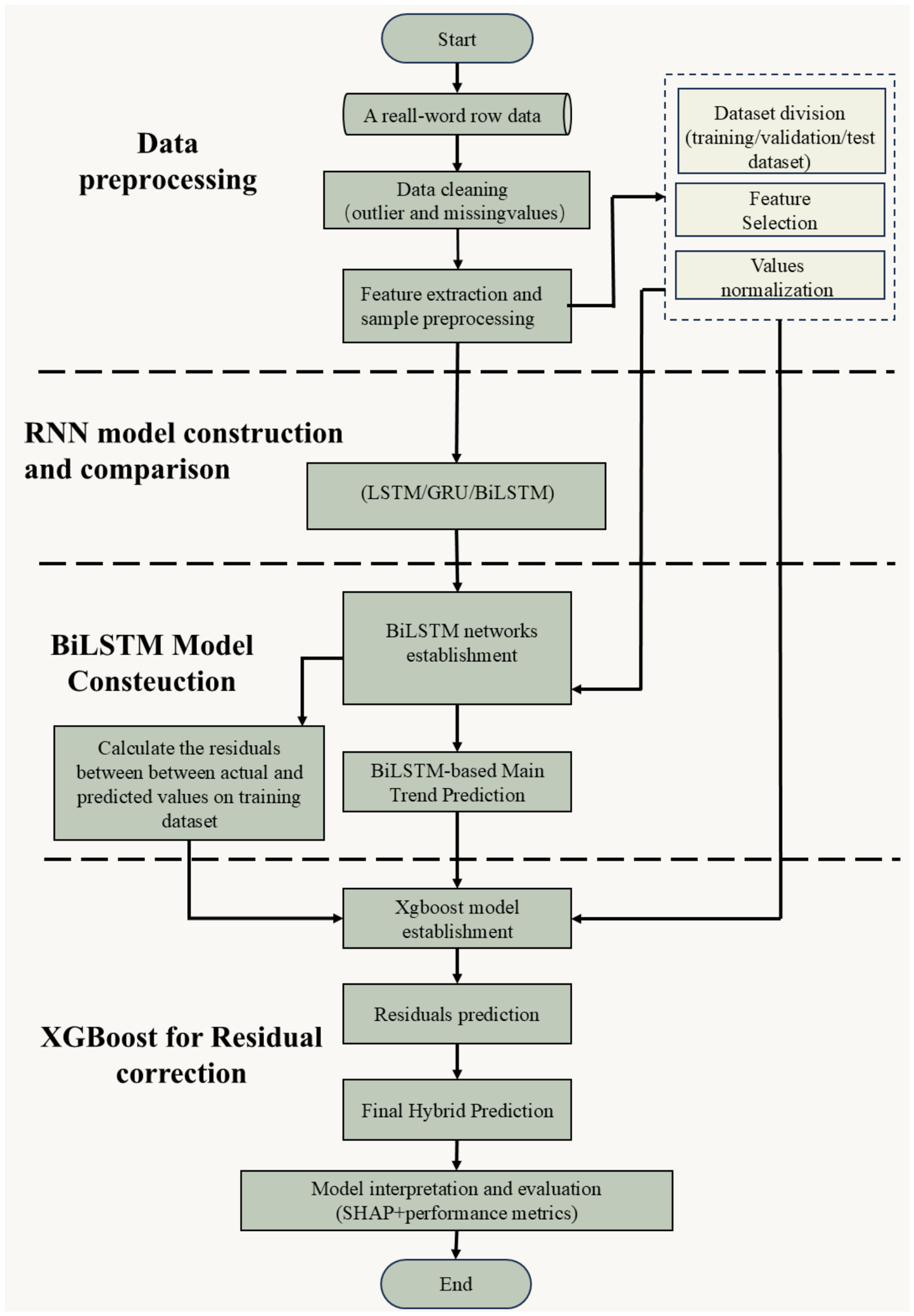
The entire runoff prediction process of the proposed method in this study is shown in Figure 1. To ensure data quality, the first step is to clean up the collected runoff and related hydrological time series data, including removing outliers and handling missing values. In the data preparation step, the Pearson correlation coefficient is used to analyze the correlation between candidate input variables and target runoff, and historical sequences that are basically related to the current runoff are selected as model input features. Then, by using the autocorrelation function (ACF) and cross-correlation (CCF) to analyze the correlation structure and lag characteristics of the runoff time series, the temporal dependence of the runoff series is characterized. This analysis lays the foundation for the input lag setting and structural construction of recurrent neural network models. In order to systematically evaluate the performance differences of various RNN structures in runoff prediction under the same data conditions, we construct and compare three common recurrent neural network models—gated recurrent unit (GRU), long short-term memory network (LSTM), and bidirectional long short-term memory network (BiLSTM). Based on the comparison results, the most suitable RNN structure is selected for studying daily runoff prediction in the watershed. This serves as the fundamental model for capturing the main temporal characteristics and patterns of runoff sequences. This study introduces a residual-learning technique to further address system biases that may occur in nonstationary processes and peak modifications of the base model: by first constructing a residual sequence based on the error between observed values and base model projection values, a “two-stage” hybrid prediction framework is created. Next, XGBoost is used to model and correct the nonlinear structure of the residuals. The basic model prediction and residual correction jointly establish the final prediction result, which improves flexibility and resistance to drastic and minor changes while retaining the ability to describe the main trends. In addition to conventional evaluation metrics, the Kruskal–Wallis (KW) test and one-sample t-test were further employed to evaluate the statistical consistency between simulated and observed runoff series. The KW test was used to examine whether the observed and predicted runoff sequences originated from the same distribution, while the one-sample t-test was applied to determine whether the mean residual significantly deviated from zero, thereby identifying potential systematic overestimation or underestimation. All models were implemented using Python 3.8.12. The BiLSTM model was developed using TensorFlow 2.10.0, and hyperparameter tuning was conducted using Keras Tuner. The residual correction model was implemented using XGBoost 2.0.3.

2.1. Date Preprocessing

Pretreatment and preliminary analysis were performed on the original runoff and associated hydrological time series data to guarantee data quality and provide the groundwork for establishing the input structure of the subsequent model. Prior to identifying outliers and handling missing values, the collected runoff data were cleaned up (Section 3.2). By identifying abnormal fluctuations and missing records, invalid data points were removed in order to reduce the influence of noise on the model training procedure.

In Pearson correlation analysis, the null hypothesis assumes that there is no linear association between meteorological variables and daily runoff ($H_0$:$\rho =0$), while the alternative hypothesis assumes a significant linear relationship ($H_1$:$\rho \ne 0$). Pearson correlation was used as a preliminary screening tool rather than for causal inference. Based on this, the linear correlation between the potential historical sequence and the current runoff was analyzed using the Pearson correlation coefficient to exclude input features that were highly correlated with the target runoff. The Pearson correlation coefficient can be calculated using the following formula:

$$r={\displaystyle \frac{{\displaystyle {\sum }_{i=1}^n(x_i-\overline{x})(y_i-\overline{y})}}{\sqrt{{\displaystyle {\sum }_{n-1}^n{(x_i-\overline{x})}^2}}\sqrt{{\displaystyle {\sum }_{n-1}^n{(y_i-\overline{y})}^2}}}}$$

(1)

where r is the correlation coefficient between variable $x$ = {$x_i$} (1 ≤ i ≤ n) and variable $y$ = {$y_i$} (1 ≤ i ≤ n). r > 0 indicates a positive correlation between variable $x$ and $y$, r < 0 indicates a negative correlation between the two, and r = 0 indicates no correlation between the two; $x_i$ is the measured value of variable $x$ at position i; $\overline{x}$ is the mean of variable $y$; $y_i$ is the measured value of variable $y$ at position i; is the mean of variable $y$; and n is the number of variables $x$ or $y$ (referred to as the time window scale in this article).

Subsequently, to further analyze the time-dependent characteristics and potential lag structures of the runoff time series, the autocorrelation function (ACF) and cross-correlation (CCF) were introduced for statistical analysis of the runoff series. ACF is used to characterize the degree of correlation between runoff sequences with different lag orders, while CCF is used to identify direct correlations after excluding intermediate lag effects. Through ACF and CCF analysis, the memory characteristics and main lag range of the runoff sequence can be preliminarily determined, providing a reference for setting the input time step in the recurrent neural network model.

2.2. Construction and Comparison of RNN Models

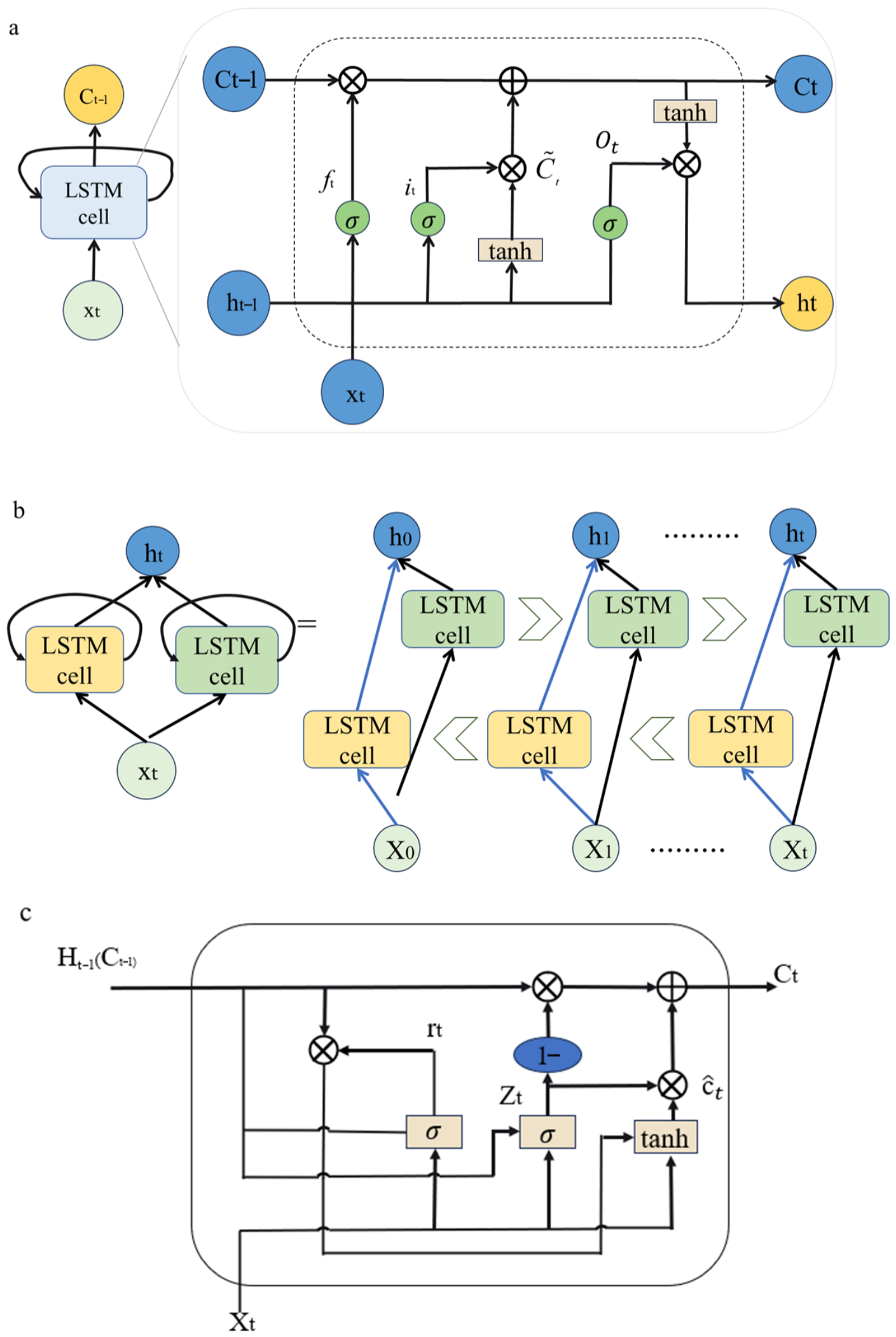
On the basis of completing data preprocessing and time-dependent structure analysis, multiple recurrent neural network (RNN) models were constructed and compared to systematically evaluate the applicability of different network structures in daily runoff prediction. As shown in Figure 2, this study selected three typical RNN architectures—long short-term memory network (LSTM), gated recurrent unit (GRU), and bidirectional long short-term memory network (BiLSTM)—and compared their predictive performance under the same data conditions and evaluation criteria.

Hochreiter and Schmidhuber [26] proposed long short-term memory (LSTM) neural networks in 1997 as an advanced iteration of recurrent neural networks (RNNs). They effectively address the issues of gradient vanishing and gradient explosion that often arise when training traditional RNNs on long sequential data. Figure 2a illustrates the LSTM model, which integrates gating mechanisms (including an input gate, a forget gate, and an output gate) to encapsulate long-term memory relationships. This design significantly enhances its ability to process long-time sequence data.

The basic equations of the LSTM model are as follows [27]:

$$\mathrm{Forget}\mathrm{Gate}:f_t=\sigma (W_f\cdot [h_{t-1},x_t]+b_f)$$

(2)

$$\mathrm{Input}\mathrm{Gate}:i_t=\sigma (W_i\cdot [h_{t-1},x_t]+b_i)$$

(3)

$$\mathrm{Cell}\mathrm{state}:C_t=f_t\otimes C_{t-1}+i_t\otimes {\tilde{C}}_t$$

(4)

$$\mathrm{Cell}\mathrm{State}\mathrm{Update}:{\tilde{C}}_t=\tanh (W_c\cdot [h_{t-1},x_t]+b_c)$$

(5)

$$\mathrm{Output}\mathrm{Gate}:O_t=\sigma (W_O\cdot [h_{t-1},x_t]+b_O)$$

(6)

$$h_t=o_t\tanh (C_t)$$

(7)

where $f_t$, $i_t$, $o_t$, ${\tilde{C}}_t$, and $h_t$ denote the forget gate, input gate, output gate, output node, memory unit, and hidden layer, respectively. $h_{t-1}$ denotes the short-term memory content from the preceding moment; $C_{t-1}$ signifies the accumulated long-term memory within the memory unit at the prior time; $W_f$, $W_i$, $W_c$, and $W_o$ represent the weight matrices; $b_f$, $b_i$, $b_c$, and $b_o$ indicate the bias vectors; $\sigma$ refers to the sigmoid function; $x_t$ is the input data, and $\tanh (C_t)$ represents the tanh activation function.

Gated recurrent unit (GRU) is another variant of RNN architecture that solves short-term memory problems and provides a simpler structure than LSTM. The LSTM network was first proposed in 1997 for language processing and is known for its excellent ability to remember long-term and short-term dependencies (Hochreiter and Schmidhuber [26]). However, due to the complex structure of LSTM neural networks, their training process usually requires a long time. To accelerate the training process, the GRU network was proposed as a modification of the LSTM network with a simpler structure [28].

In the GRU structure shown in Figure 2c, the calculation of the update equation is as follows:

$$r_t=\sigma (W_{xr}{x}_t+W_{hr}{h}_{t-1}+b_r)$$

(8)

$$Z_t=\sigma (W_{xz}{x}_t+W_{hz}{h}_{t-1}+b_z)$$

(9)

$${\widehat{c}}_t=\tanh (W_{xc}{x}_t+W_{hc}(r_t\otimes h_{t-1})+b_c)$$

(10)

$$c_t=(1-Z_t)\otimes c_{t-1}+Z_t\otimes {\widehat{c}}_t$$

(11)

$$h_t=c_t$$

(12)

where $W_{xr}$, $W_{hr}$, $W_{xz}$ and $W_{hc}$ are the weight matrices of the network; $b_r$ and $b_z$ are bias vectors; and $r_t$ and $Z_t$ are the activation value vectors corresponding to the reset gate and update gate, respectively.

Due to the influence of human activities and meteorological changes, the daily demand for runoff water usually exhibits different regularities. The prediction of daily runoff depends on its past meteorological data and the impact of human activities, and it also has a reverse effect on the runoff in subsequent time periods. In this regard, we adopt the BiLSTM network architecture to extract periodic features and capture this temporal dependence from historical meteorological data. The structure of a BiLSTM network consists of two separate LSTM layers, one stacked on top of the other, with one processing input data in a forward pass and the other processing input data in a backward pass. This configuration allows learning forward and backward data. Figure 2b provides an overview of the BiLSTM network structure used in our model.

Through the above comparative analysis, the RNN structure that performs relatively better under the conditions of this study was determined, and it was used as the basic model for the subsequent residual learning and mixed modeling stages.

2.3. Residual Learning with XGBoost

The LSTM network effectively captures the long-term dependencies of time series through a gating mechanism, while XGBoost is based on a gradient boosting decision tree and uses second-order Taylor expansion to approximate the loss function, thereby minimizing the objective function more accurately in each iteration. BiLSTM is trained on the training set, the prediction ${\widehat{y}}_t^{\mathrm{BiLSTM}}$ is obtained, and the residual is calculated:

$$r_t=y_t-{\widehat{y}}_t^{\mathrm{BiLSTM}}$$

(13)

where the variable represents the actual residual that can be calculated from the training set, reflecting the partial relationship that BiLSTM failed to capture.

The residual obtained from the training set and the meteorological data processed through sample processing and feature processing are fed into XGBoost for residual correction. The calculation formula for the final residual-correction result is as follows:

$${\hat{r}}_t=f_{\mathrm{XGBoost}}(z_t)\approx E[r_t|z_t]$$

(14)

After the model training is completed, XGBoost relies only on input features and BiLSTM output for inference in the prediction stage:

$${\widehat{y}}_t={\widehat{y}}_t^{\mathrm{BiLSTM}}+{\widehat{r}}_t^{\mathrm{XGBoost}}$$

(15)

where ${\widehat{r}}_t^{\mathrm{XGBoost}}$ is the estimated residual value of XGBoost.

To thoroughly assess the ability of various sequence models in capturing runoff dynamics, several representative recurrent neural network architectures were chosen for comparison, including LSTM, GRU, and BiLSTM. LSTM is commonly utilized in hydrological modeling because of its capacity to capture long-term dependencies and alleviate issues with gradient disappearance. GRU features a simpler gating structure, which provides computational efficiency and has demonstrated competitive performance in time-series prediction. BiLSTM enhances the standard LSTM by incorporating bidirectional information flow, potentially improving feature representation when adequate temporal context is available. However, these RNN-based models may still face challenges in addressing residual nonlinearities and systematic biases, which underscores the need for integrating tree-based learners like XGBoost for correcting residuals, particularly in scenarios where the data exhibits complex patterns that RNNs struggle to capture effectively.

2.4. Evaluation Results

To evaluate the correctness and reliability of the model simulation outputs, numerous statistical variables prevalent in hydrology were used to determine the predictive dependability of each model [29]. This study selected four metrics for complete evaluation: Nash–Sutcliffe efficiency coefficient (NSE), root mean square error (RMSE), coefficient of determination (R²), and mean absolute error (MAE). The NSE assesses the model’s goodness of fit to the observed data, with values approaching 1 indicating superior predictive performance. RMSE and MAE evaluate the model’s predictive accuracy through error distribution and average deviation, respectively, with RMSE being more responsive to larger errors. The MAE indicates the mean discrepancy between the expected and observed values.

The formulas are as follows:

$$\mathrm{NSE}=1-{\displaystyle \frac{{\displaystyle {\sum }_{\mathrm{i}=1}^{\mathrm{n}}({\mathrm{y}}_i-\hat{\mathrm{y}}{)}^2}}{{\displaystyle {\sum }_{i=1}^n{({\mathrm{y}}_i-\stackrel{\_}{y})}^2}}}$$

(16)

$$\mathrm{RMSE}=\sqrt{{\displaystyle \frac{1}{n}}{\displaystyle \sum _{i=1}^n{(\widehat{y}-y_i)}^2}}$$

(17)

$$\mathrm{MAE}={\displaystyle \frac{1}{n}}{\displaystyle \sum _{i=1}^n\left|\hat{\mathrm{y}}-y_i\right|}$$

(18)

$${\mathrm{R}}^2=1-{\displaystyle \frac{{\displaystyle {\sum }_{\mathrm{i}=1}^n{(y_i-{\widehat{y}}_i)}^2}}{{\displaystyle {\sum }_{i=1}^n}{(y_i-{\overline{y}}_i)}^2}}$$

(19)

where n is the number of sanples; $y_i$ is the observed value; $\stackrel{\_}{y}$ is the mean of the $y$; ${\widehat{y}}_i$ is the predicted value.

According to the relevant provisions of “Hydrological Intelligence Specification” [30], when 0.90 ≤ NSE, the prediction accuracy is class A; when 0.70 ≤ NSE < 0.90, the prediction accuracy is class B; when 0.05 ≤ NSE < 0.70, the prediction accuracy is class C; and when NSE < 0.50, the prediction result is not credible.

3. Case Study

3.1. Study Area

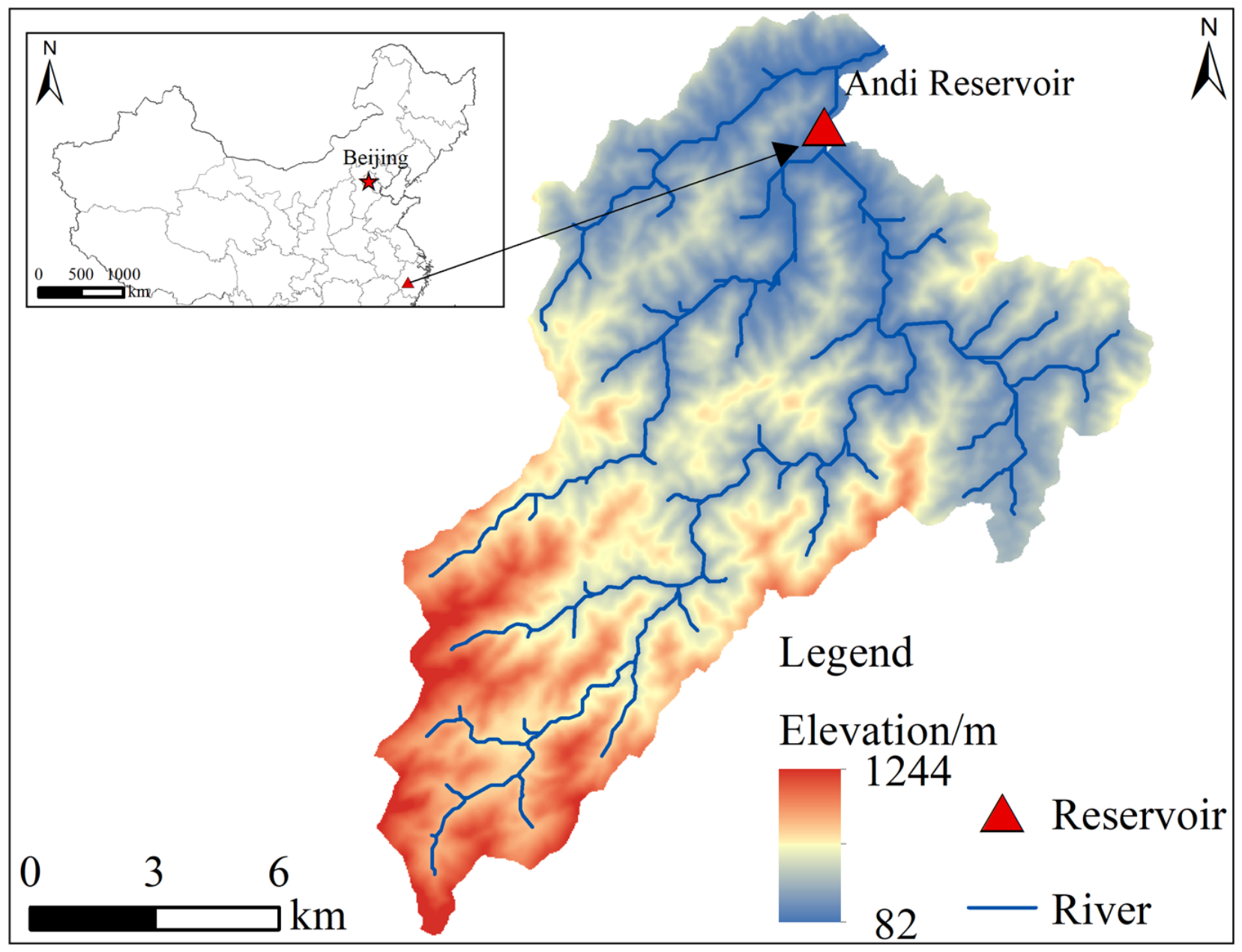
The Andi Reservoir is in the upper reaches of the Meixi River Basin in Jinhua City, Zhejiang Province (Figure 3). It has a water area of 3.42 km², a catchment area of 162 km², and an elevation of 126.5 m [31]. It is one of the main drinking water sources in Jinhua City. The catchment area of Andi Reservoir’s terrain is high in the southwest and low in the southeast, with elevations ranging from 82 to 1244 m. The terrain shifts from the southwest to the northeast. The Andi Reservoir is situated within the subtropical monsoon climate zone, a region characterized by significant seasonal variations in climate. The mean annual rainfall and temperature were 1664.4 mm and 17.34 °C, respectively. And the mean annual potential evapotranspiration is 1114.2 mm. The daily runoff data used in this study come from the monitoring station for runoff at Andi, which is located near the upstream river section of the Andi Reservoir watershed (Figure 3).

3.2. Data Sources

In this study, an empirical analysis was conducted using meteorological data extracted from the ERA5 dataset (ERA5-Land Hourly–ECMWF Climate [32])—including rainfall, average temperature, average relative humidity, average wind speed, average daily radiation, NDVI, and slope—along with daily runoff data from the Andi Reservoir in Jinhua, Zhejiang Province, spanning the period from 2016 to 2023 and totaling 2883 daily runoff records. All runoff measurements correspond to the same time of day at the reservoir monitoring station.

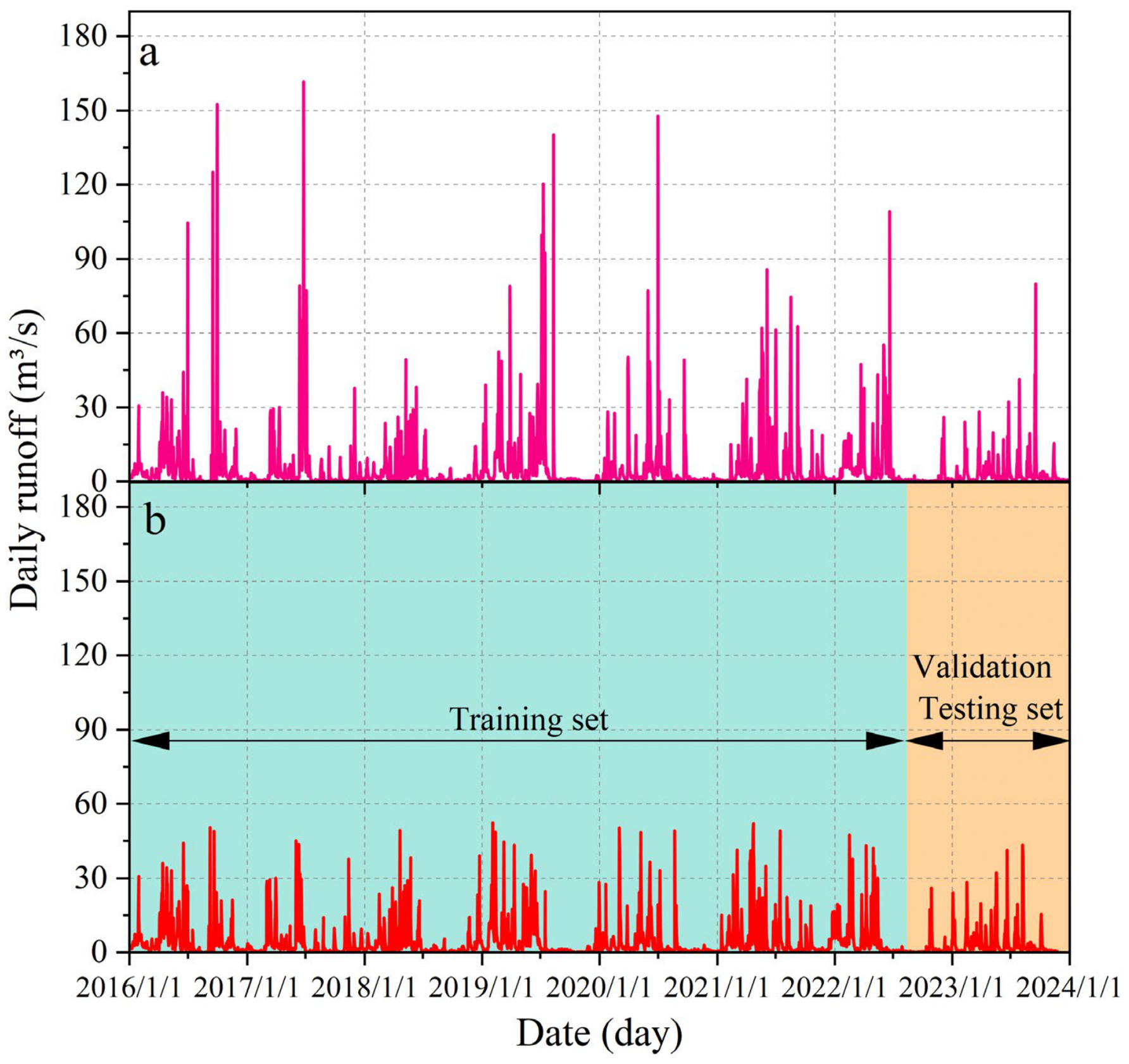
To reduce the interference of outliers in the model training, the negative values of the daily runoff data were removed, and more than 99% of the quantiles (extremely large values) were excluded. The result is shown in Figure 4. The dataset was divided according to the ratio of 8:2, with the first 2307 days of water level data as the training set and the last 576 days of water level data as the validation set. The model presented in this paper, as well as the comparison model, is validated using both the training set and the validation set. Although a chronological split was adopted, the training period spans multiple years and covers all seasons with comparable proportions, ensuring that the model is trained under diverse seasonal conditions rather than being biased toward a specific season. The proposed model and the comparison models were trained and evaluated using the same training and validation datasets.

3.3. Pearson Correlation Analysis Between Meteorological Factors and Runoff

The Pearson correlation coefficient was calculated as described in Section 2.1. To explore the linear relationship between meteorological factors and runoff, the Pearson correlation coefficient was used to analyze the relationship between various meteorological variables and daily runoff. The results are shown in

Table 1. Pearson correlation calculation results for meteorological factors.

Factor	r	p
Rainfall	0.344	0.0001
Soil moisture	0.347	0.0001
Solar radiation	−0.230	0.0001
Wind speed	−0.108	0.005
Temperature	−0.028	0.2315

. There is a significant positive correlation between rainfall, soil moisture, and runoff (r = 0.344 and 0.347, respectively), indicating that an increase in rainfall or soil moisture usually leads to an increase in runoff. There is a significant negative correlation between daily solar radiation, wind speed, and runoff (r = −0.230 and −0.108, respectively), p < 0.005. This suggests that higher levels of solar radiation and wind speed encourage evaporation, which in turn decreases runoff. The correlation between temperature and runoff is not significant (p > 0.05), indicating that the direct impact of temperature changes on daily runoff in the study area is relatively small. Overall, rainfall and soil moisture are the main driving factors for runoff changes, while solar radiation and wind speed also have a significant inhibitory effect on runoff.

3.4. Autocorrelation and Partial Autocorrelation Analysis of Runoff Series

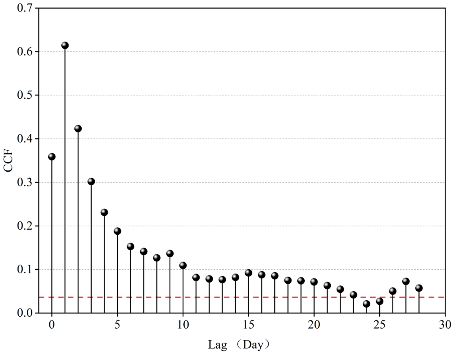
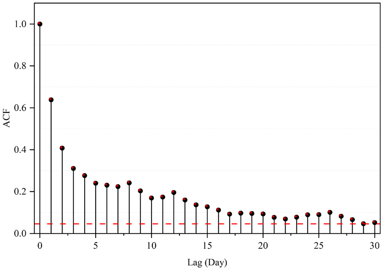
This article examined the cross-correlation function (CCF) between rainfall and runoff (Figure 5) and the autocorrelation function (ACF) of runoff (Figure 6) to investigate the temporal dependency of runoff and its delayed response to rainfall.

ACF shows that there is a strong positive correlation between runoff in orders 1–7, a moderate correlation in orders 8–15, and a significant but weak correlation at around order 20; CCF analysis reveals that the runoff response to rainfall peaks after a 1-day lag, signifying that the watershed exhibits a rapid and direct reaction to rainfall input. The substantial connection is most evident in the initial days; however, it persists as a weak, non-zero correlation over an extended lag period, illustrating the cumulative influence of prior conditions and the nonlinear propagation traits in the rainfall runoff process.

The detailed findings of ACF and CCF demonstrate that the temporal dependency of runoff is most influenced by short-term rainfall; however, it is not exclusively confined to the initial days. The selection of input lag time is not only determined by the peak correlation location but must also encompass the effective temporal range indicated by correlation analysis. This article uses a 28-day input time window for the model. This lets it fully capture the main short-term response process without cutting off possible delay information too soon. It also gives the BiLSTM model enough time context to learn relevant time dependencies from the data.

3.5. Stationarity Analysis of Runoff Time Series

The stationarity of the daily runoff series was assessed using the augmented Dickey–Fuller (ADF) and KPSS tests (

Table 2. Stationarity test results for the daily runoff series.

Series	ADF Statistic	ADF p-Value	KPSS Statistic	KPSS p-Value
Runoff	−12.13	<0.05	0.120	>0.05

). The ADF test (p < 0.05) indicates a rejection of the unit-root hypothesis, while the KPSS test (p > 0.05) fails to reject the null hypothesis of level stationarity. These results suggest that the runoff series does not exhibit unit-root-type nonstationarity.

However, the absence of unit-root nonstationarity does not imply a simple or directly predictable runoff process. The time series exhibits pronounced seasonal fluctuations and abrupt changes, which are closely associated with rainfall events and watershed response dynamics, as evidenced by the correlation analysis, ACF/CCF results, and the temporal distribution of runoff peaks. Such characteristics indicate that runoff variability is governed by short-term, event-driven processes and nonlinear interactions rather than long-term trends. Therefore, nonlinear sequence models are required to capture these complex temporal dependencies, which cannot be adequately represented by linear stationary assumptions.

3.6. Model Parameter Configuration

There are several hyperparameters that need to be carefully configured for BiLSTM, LSTM, and GRU models: (1) the number of BiLSTM layers; (2) the number of neurons in each layer; (3) learning rate; (4) activation function; (5) a dropout layer. Using too many layers and neurons may create overly complex models that are challenging to train and computationally infeasible. On the contrary, overly simple settings may result in unexpected predictions. Furthermore, selecting the optimal number of training periods for the model is crucial. This study adopted an early stopping training strategy to optimize computation time by evaluating the convergence and stability of training and validation losses. In all BiLSTM, LSTM, and GRU models, we employed the Adam optimizer, which combines momentum and adaptive learning rates and has been widely used in deep learning-based hydrological forecasting due to its stable and efficient convergence on nonlinear, nonstationary time series.

To obtain the optimal performance of LSTM, GRU, and BiLSTM in runoff prediction tasks, this study systematically optimized the model hyperparameters using Keras tuner. The Keras tuner is an extensible hyperparameter optimization framework that addresses the challenges of hyperparameter search by integrating built-in Bayesian optimization, subband, and random search algorithms. Compared with traditional grid search and manual search, random search constitutes a more effective hyperparameter optimization method [33]. We use mean square error (MSE) as the evaluation metric and configure parameters within the search range to minimize MSE. We obtained the optimal parameter configuration results through three experiments using the Keras tuner, as shown in

Table 3. Hyperparameter search range and optimal configuration of the BiLSTM, LSTM, and GRU models.

Hyperparameter	Search Range	BiLSTM	GRU	LSTM
Number of layers	[2, 3]	2	1	1
Number of neurons	[32, 48, 64, 96]	64	96	48
Learning rate	ranging from 0.0001 to 0.01 with an increase of 0.0001	0.0005	0.001	0.0003
Activation	ReLU, tanh	ReLU (Dense), tanh/sigmoid	ReLU (Dense), tanh/sigmoid	ReLU (Dense), tanh/sigmoid
Dropout:	True/False	True (0.2)	True (0.5)	True (0.5)

and

Table 4. Hyperparameter search range and optimization configuration of the XGBoost model.

Hyperparameter	Search Range	XGBoost
n_estimators	ranging from 100 to 1500	1000
max_depth	[2, 3, 4, 5, 6]	3
eta	ranging from 0.0001 to 0.01 with an increase of 0.0001	0.01
gamma	[0, 1, 2, 3]	0
subsample	ranging from 0.5 to 1 with an increase of 0.1	0.6
colsample_bytree	ranging from 0.5 to 1 with an increase of 0.1	0.8

.

For the XGBoost model, the hyperparameters can be broadly grouped into three categories: (1) general parameters, (2) booster parameters, and (3) learning task parameters. General parameters specify the type of booster used for learning, typically tree-based or linear models [34].

In this study, we focus primarily on the booster parameters, as they have the most direct impact on the fitting performance among the three categories. A random search strategy is adopted to identify the optimal configuration of the key booster hyperparameters, including (1) n_estimators, (2) max_depth, (3) gamma, (4) eta (i.e., learning rate), (5) subsample, and (6) colsample_bytree. Table 4 summarizes the search ranges of these six hyperparameters and reports the optimal combination obtained for the XGBoost model. All other XGBoost parameters not explicitly listed are kept at their default settings.

3.7. Sensitivity Analysis of Key Hyperparameters

Sensitivity assessments were performed on the important hyperparameters of the BiLSTM and XGBoost components one at a time (OAT) to assess the robustness of the suggested hybrid framework and mitigate the “black box” issue commonly associated with machine learning models. While all other hyperparameters and data partitions remained unchanged in the jointly optimized configuration, one hyperparameter changed during the analysis process. The sensitivity analysis findings are shown in

Table 5. Sensitivity analysis of key hyperparameters for BiLSTM and XGBoost.

Model	Parameter	Value	NSE	RMSE
BiLSTM	Learning rate	0.01	0.4522	3.72
BiLSTM	Learning rate	0.001	0.5269	3.46
BiLSTM	Learning rate	0.0005	0.5517	3.37
BiLSTM	Dropout	0.2	0.5855	3.24
BiLSTM	Dropout	0.3	0.4633	3.68
BiLSTM	Dropout	0.4	0.5560	3.24
BiLSTM	Hidden units	32	0.5233	3.47
BiLSTM	Hidden units	64	0.5610	3.33
XGBoost	Max depth	3	0.5466	3.39
XGBoost	Max depth	5	0.5679	3.30
XGBoost	Max depth	7	0.4989	3.56

.

The learning rate substantially influences the predictive performance of the BiLSTM model. Table 5 illustrates that a comparatively high learning rate (0.01) results in diminished prediction accuracy (NSE = 0.4522, RMSE = 3.72), signifying unstable convergence. Decreasing the learning rate to 0.001 enhances model performance (NSE = 0.5269, RMSE = 3.46), while a further reduction to 0.0005 yields optimal performance in the test values (NSE = 0.5517, RMSE = 3.37). This suggests that a reduced learning rate may yield more stable optimization and enhanced generalization for the BiLSTM model in this context.

The influence of the dropout rate on BiLSTM performance does not exhibit a straightforward monotonic trend. When the dropout rate is set to 0.2, the model attains its highest performance (NSE = 0.5855, RMSE = 3.24), which indicates an optimal level of regularization. However, increasing the dropout rate to 0.3 results in a significant decline in predictive accuracy (NSE = 0.4633, RMSE = 3.68). Interestingly, when the dropout rate is further increased to 0.4, there is a partial recovery in model performance (NSE = 0.5560, RMSE = 3.24). The dropout configuration influences BiLSTM predictions, and both inadequate and excessive regularization can adversely affect model accuracy, according to these results.

The sensitivity of the BiLSTM model is quite low throughout the testing range with respect to the number of hidden units. While increasing representational power can enhance performance, the overall impact is still minimal. For example, increasing the number of units from 32 to 64 can moderately improve prediction accuracy (NSE improved from 0.5233 to 0.5610, and RMSE fell from 3.47 to 3.33).

The maximum tree depth for the XGBoost residual-correction module underwent a sensitivity analysis. A medium tree depth of 5 yielded the best results, with an NSE of 0.5679 and an RMSE of 3.30, as shown in Table 5. However, using very deep trees (depth = 7) led to a performance decline (NSE = 0.4989, RMSE = 3.56), indicating potential overfitting. In contrast, shallow trees (depth = 3) performed worse than the residual structures, with an NSE of 0.5466 and an RMSE of 3.39. These findings suggest that effective residual correction requires careful control of model complexity.

4. Results

4.1. Comparative Analysis of Model Prediction Performance

In this study, four daily runoff prediction models based on LSTM, GRU, BiLSTM, and BiLSTM–XGBoost hybrid are constructed, respectively, and their performances on the test set are comprehensively compared using evaluation metrics such as root mean square error (RMSE), mean absolute error (MAE), coefficient of determination (R²), and Nash–Sutcliffe efficiency coefficient (NSE). The evaluation results of each model on the test set are shown in

Table 6. Performances of each model.

Model	Dataset	RMSE	MAE	NSE	R2
LSTM	Testing	3.45	1.40	0.53	0.53
BiLSTM	Testing	3.16	1.20	0.61	0.59
GRU	Testing	3.35	1.31	0.55	0.56
BiLSTM–XGBoost	Testing	1.82	0.76	0.86	0.86

.

From Table 6, it can be seen that BiLSTM, GRU, and LSTM models can all reproduce the overall trend of runoff processes well, but there are significant differences in prediction accuracy. The BiLSTM model performs the best, with a testing RMSE of 3.16 m³/s, MAE of 1.20 m³/s, and NSE and R² of 0.61 and 0.59, respectively. The RMSE and MAE of the LSTM model are 3.45 m³/s and 1.40 m³/s, respectively, with an R² of 0.53; the RMSE and MAE of the GRU model are 3.35 m³/s and 1.31 m³/s, respectively, with an R² of 0.56. Compared to the LSTM model, the RMSE of BiLSTM decreased by about 8.4%, MAE decreased by about 14.3%, and R² increased by about 11.3% (from 0.53 to 0.59); compared to the GRU model, the RMSE of BiLSTM decreased by about 5.7%, MAE decreased by about 8.4%, and R² increased by about 5.4%. BiLSTM outperforms the other two unidirectional structural models in terms of overall error, goodness of fit, and correlation and can more fully capture nonlinear features and temporal dependencies in daily runoff sequences.

From the comparison of the runoff process in Figure 7, it can be further observed that the LSTM model exhibits significant lag and underestimation during the peak stage, with insufficient capture of fluctuations in peak duration and low flow stage (Figure 7a); the GRU model shows slight improvement in prediction at the peak time but still exhibits some smoothing deviation on the rising and falling edges (Figure 7b). In contrast, the predicted curve of the BiLSTM model is more consistent with the measured data in terms of peak amplitude and temporal position and can better capture the rapid fluctuations and multi-peak characteristics of flood processes (Figure 7c). In Figure 7d, the BiLSTM–XGBoost hybrid model further enhances the agreement with the observed runoff process. High-flow events are more accurately represented in both magnitude and duration, while low-flow periods exhibit reduced random fluctuations. Overall, the hybrid model shows the closest correspondence to the observed hydrograph across different flow regimes.

4.2. Analysis of Prediction Trends and Residual Distributions

This study enhances prediction accuracy and addresses the limits of a single deep learning model in capturing intricate nonlinear interactions by including XGBoost for residual correction based on the BiLSTM model, thereby constructing a hybrid model, BiLSTM–XGBoost. This approach initially employs BiLSTM for primary prediction of the runoff time series, subsequently training the XGBoost model using the residuals (the discrepancy between observed and anticipated values) as input features, thus facilitating secondary learning and rectification of systematic errors.

Figure 8 shows the scatter comparison between the predicted and measured values of LSTM, GRU, BiLSTM, and BiLSTM–XGBoost models. It can be seen that the point cloud distribution of the hybrid model (Figure 8c) is the most concentrated and closest to the ideal 1:1 line, indicating that its overall fitting performance is significantly better than the other three single models. The fitting equation of the BiLSTM–XGBoost model is y = 0.28 + 0.94x, with the slope closest to 1 and the intercept closest to 0, indicating that the model’s prediction error is minimal and the system bias is significantly reduced. From Table 6, it can be seen that the RMSE of the BiLSTM–XGBoost model is 1.82 m³/s, the MAE is 0.76 m³/s, the NSE is 0.86, and the R² is 0.86. Compared with the single BiLSTM model (RMSE is 3.16 m³/s, MAE is 1.20 m³/s, NSE is 0.61, and R² is 0.59), the performance has been significantly improved. Specifically, RMSE decreased by about 42.4%, MAE decreased by about 36.7%, NSE increased by 41.0%, and R² increased by about 45.8%. As shown in Figure 8b,d, the LSTM and GRU models exhibit widely dispersed points and significant deviations from the 1:1 line, especially in the medium- to high-flow range, where predicted values are generally lower than observed values, indicating a systematic underestimation phenomenon. In Figure 8a, the BiLSTM model shows that compared to LSTM and GRU, the point concentration around the 1:1 line has improved, and the dispersion has decreased in most flow ranges. However, at higher runoff values, dispersion remains evident, indicating that prediction uncertainty is still significant under high-flow conditions. Compared with LSTM (Figure 8b) and GRU (Figure 8d), the hybrid model not only significantly improved the fitting accuracy but also significantly reduced the number of discrete points in the high-flow stage, demonstrating better generalization performance and stability.

4.3. An Explanation of the Importance of Features in the XGBoost and BiLSTM Model

This study uses the Shapley Additive Explanations (SHAP) method to conduct interpretability analysis on the BiLSTM–XGBoost model to further explore how to improve the predictive performance of hybrid models and verify the rationality of the model’s internal decision-making process. SHAP can quantify the importance and impact direction of different variables on the model output by calculating the marginal contribution of each input feature to the prediction results, thereby revealing the internal mechanism of the model in learning runoff variation patterns.

Figure 9 shows the SHAP analysis results of the top ten main influencing factors of the BiLSTM–XGBoost model. From the global feature importance ranking in Figure 9a, it can be seen that BiLSTM Prediction and BiLSTM Residual are the two most critical variables that affect the model output, with significantly higher average SHAP values than other features. Figure 9b’s SHAP summary diagram further illuminates the positive and negative impacts of each feature on the predicted values. Overall, the BiLSTM predicted values and BiLSTM residuals correspond to positive SHAP values when they are high, which will push up the runoff predicted by the model. This indicates that the second-stage XGBoost will further amplify the runoff response when the BiLSTM prediction is large or there is a positive residual, thereby improving the peak simulation effect. In contrast, the interaction term between temperature and radiation often exhibits negative SHAP values in high-value areas, which have a suppressive effect on runoff, consistent with the hydrological process of enhanced evapotranspiration and unfavorable runoff formation under high temperature and strong radiation conditions.

Figure 10 shows the distribution of SHAP values for each input variable in the BiLSTM model, which intuitively reflects the positive and negative impact directions and contribution strengths of each feature on the prediction results. Figure 10a shows the average |SHAP| values of the top 10 important features of BiLSTM; Figure 10b shows the SHAP summary scatter plot for the same feature set. Overall, the model is most sensitive to short-term hydrological memory and recent humidity rainfall conditions: the interaction term “rainfall x relative humidity” contributes the most, and the SHAP values corresponding to the high values (red) in Figure 10b are mostly positive, indicating that when the air humidity is high and rainfall occurs, the model tends to significantly increase the predicted runoff. The second is the extreme inflow value (rolling max) in the recent 3 and 7 days, and the SHAP value of the strong rainfall indicator variable is mainly distributed in the positive half-axis, indicating that the rainstorm event will significantly increase the prediction; the cumulative rainfall over 3 and 7 days both contribute positively to the shallow soil moisture content, while the average impact of solar radiation and seasonal terms (monthly sine) on the prediction is relatively small, but the direction is stable. This indicates that BiLSTM mainly characterizes runoff processes through short-term water input and the underlying surface and achieves a unified characterization of peak and steady periods under the modulation of energy conditions (radiation) and a seasonal background.

4.4. Statistical Consistency Analysis Between Model Predictions and Observed Runoff

To further evaluate the consistency between simulated runoff and observed runoff, this study used the Kruskal–Wallis (KW) nonparametric test and the single-sample t-test on the test set to statistically validate four models (LSTM, GRU, BiLSTM, and BiLSTM–XGBoost). The Kruskal–Wallis test is used to determine whether the predicted and observed sequences of each model come from the same distribution to evaluate the statistical compatibility of the model at the population distribution level; the single-sample t-test is used to evaluate whether the mean residual of the model deviates significantly from zero to identify whether the model has systematic overestimation or underestimation. The relevant results are summarized in

Table 7. Summary of Kruskal–Wallis and one-sample t-test results for statistical consistency between simulated and observed runoff.

Model	Statistic	p-Value	Critical Value	H0 (Compatibility/No Bias)
LSTM	H = 3.40	0.0652	0.05	Accept
BiLSTM	H = 16.20	5.71 × 10−5	0.05	Reject
GRU	H = 14.87	1.15 × 10−4	0.05	Reject
BiLSTM–XGBoost	H = 1.06	0.3024	0.05	Accept
LSTM	t = −1.71	0.0869	0.05	Accept
BiLSTM	t = −2.25	0.0247	0.05	Reject
GRU	t = 0.65	0.5138	0.05	Accept
BiLSTM–XGBoost	t = −1.34	0.1809	0.05	Accept

.

The null hypothesis (H₀) of the Kruskal–Wallis test is that the observed sequence and the predicted sequence of the model come from the same distribution. When p > 0.05, this hypothesis cannot be rejected, indicating that the simulated runoff in the model is consistent with the observed values in the overall distribution. As shown in Table 7, the p-values of LSTM, BiLSTM-XGBoost are 0.0652 and 0.3024, respectively, all greater than 0.05, indicating statistical consistency with observed runoff in the overall distribution. On the contrary, the p-values of BiLSTM and GRU are 5.71 × 10⁻⁵ and 1.15 × 10⁻⁴, respectively, which are significantly less than 0.05, indicating a significant distribution difference between their predicted and observed sequences and insufficient statistical compatibility.

The null hypothesis H₀ of the single-sample t-test is that the mean residual of the model is zero, indicating that there is no systematic bias in the model. When p > 0.05, there is no significant difference between the residual mean and zero, indicating that the model is consistent with the observation in terms of mean. From Table 7, it can be seen that the p-values of LSTM, GRU, and BiLSTM–XGBoost are 0.0869, 0.5138, and 0.1809, respectively, all greater than 0.05. Therefore, none of these three models exhibits systematic overestimation or underestimation. The p-value of BiLSTM is 0.0247, less than 0.05, and its t-statistic is negative (−2.25), indicating significant systematic underestimation of the model.

5. Discussion

This study rigorously evaluated the effectiveness of four deep learning models—LSTM, GRU, BiLSTM, and the residual-driven BiLSTM–XGBoost hybrid framework—in predicting daily runoff. The research adopts a systematic analysis method that encompasses the entire process, from data diagnosis to model interpretability. Recent data-driven hydrological studies [35] widely utilize a similar step-by-step approach, beginning with screening predictive factors and identifying dependencies, followed by model evaluation. Before building the models, the Pearson correlation analysis shown in Table 1 is often used to check how well runoff and possible predictive factors are linearly related. The moderate correlation strength observed in this study aligns with findings from previous research, suggesting that linear correlation alone cannot completely account for changes in runoff, particularly in event-driven watersheds [36]. This observation underscores the need for nonlinear modeling methods.

An extensive examination of temporal dependence was performed using autocorrelation (ACF) (Figure 6) and cross-correlation (CCF) analysis (Figure 5), revealing that the correlation demonstrated significant short-term persistence, which quickly diminished with increasing lag. This behavior is consistent with preliminary research indicating that daily runoff is primarily influenced by short-term memory and initial humidity conditions [37,38]. Considering the comprehensive decay structure—rather than solely the initial correlation peak—a 28-day input window was chosen to retain delayed yet hydrologically meaningful information. This approach differs from methods that determine lag length based only on the initial maximum correlation value. It adheres to contemporary recommendations by considering the broader effective time dependence suggested by the decay mode, thereby preventing premature truncation of the main effect. Although the ADF and KPSS test results in Table 2 suggest that the runoff sequence does not exhibit unit-root nonstationarity, this finding is consistent with numerous daily runoff records documented in the literature [39,40]. The presence of seasonality, mutations, and extremes highlights the necessity for nonlinear sequence models that can effectively handle structurally complex yet statistically stable sequences.

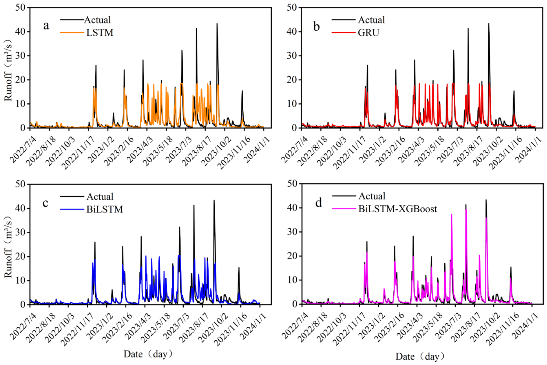
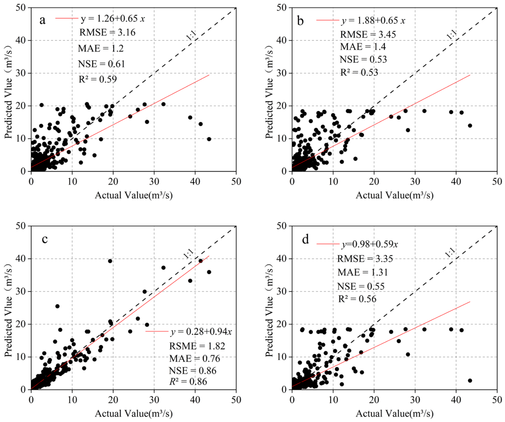
Among the single recurrent neural network models, LSTM and GRU were able to reproduce the general runoff trend but exhibited notable smoothing and underestimation of flood peaks (Figure 7a,b and Figure 8b,d), a limitation that has been widely documented in previous rainfall–runoff modeling studies [41,42]. The BiLSTM model demonstrated superior performance among the single models, outperforming LSTM and GRU in capturing peak arrival time, fitting hydrograph dynamics, and improving deterministic evaluation metrics (RMSE, MAE, NSE, and R²) (Figure 7c and Figure 8a). This improvement is consistent with published evidence showing that bidirectional architectures can better exploit temporal context and improve peak representation in flood prediction tasks [43,44]. Nevertheless, Table 7 statistical consistency analysis revealed that BiLSTM predictions still exhibited significant distributional differences from observations (Kruskal–Wallis test p < 0.05) and a negative residual mean (t-test p = 0.0247), indicating systematic underestimation despite improved trend fitting.

In order to address the limitations of BiLSTM model in representing highly nonlinear responses and local fluctuations, an extreme gradient boosting ensemble model was introduced to learn and correct the residuals generated by BiLSTM model, forming a two-stage BiLSTM–XGBoost hybrid framework. The use of gradient enhancement as a residual corrector follows the increasing trend of mixed modeling research in hydrology, where second-order learners are used to capture structural errors left by sequential models [45]. In this structure, the BiLSTM model is responsible for learning the main runoff evolution, while the extreme gradient boosting is used for targeted correction of flood peaks, abrupt changes, decay, and high-frequency nonlinear signals (Figure 7d and Figure 8c). Compared with a single BiLSTM model, the hybrid framework achieved substantial improvements, with RMSE and MAE reduced by about 40% and NSE and R² increased by about 0.27 (Table 6). These performance gains are comparable to those reported in previous mixed runoff and environmental prediction studies, confirming the effectiveness of residual-driven correction.

The optimized hyperparameter configurations summarized in Table 3 and Table 4 further support the robustness of the proposed modeling framework. As shown in Table 3, all recurrent neural network models converge to relatively shallow architectures with moderate neuron numbers, indicating that daily runoff dynamics can be effectively captured without excessive network depth or width. In particular, the BiLSTM model achieves optimal performance with a compact structure, suggesting that its superiority primarily stems from the bidirectional temporal learning mechanism rather than increased model complexity. Similar conclusions have been reported in previous runoff modeling studies, where moderate network complexity was found sufficient for daily-scale prediction tasks [42,46]. Table 4 shows that the XGBoost model adopts a conservative boosting strategy characterized by a small learning rate and moderate tree complexity. This configuration enables gradual and stable correction of residual errors, reducing the risk of overfitting while enhancing local prediction accuracy. Such parameter settings are consistent with earlier hybrid modeling studies, which emphasize that tree-based learners are most effective when used as residual correctors rather than standalone predictors in hydrological applications [47].

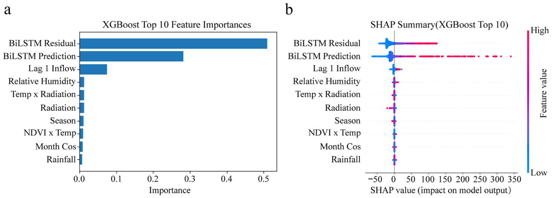
The interpretability analysis utilizing SHAP offers mechanical insights to enhance the efficacy of hybrid frameworks. Recent applications of interpretable machine learning in hydrology utilize SHAP to differentiate the functions of two modeling phases [48,49]. The SHAP results in Figure 9 for the BiLSTM–XGBoost model demonstrate that BiLSTM predictions, residual information, and previous runoff are the primary determinants of feature importance, affirming that the second-level XGBoost functions primarily as a nonlinear error corrector. 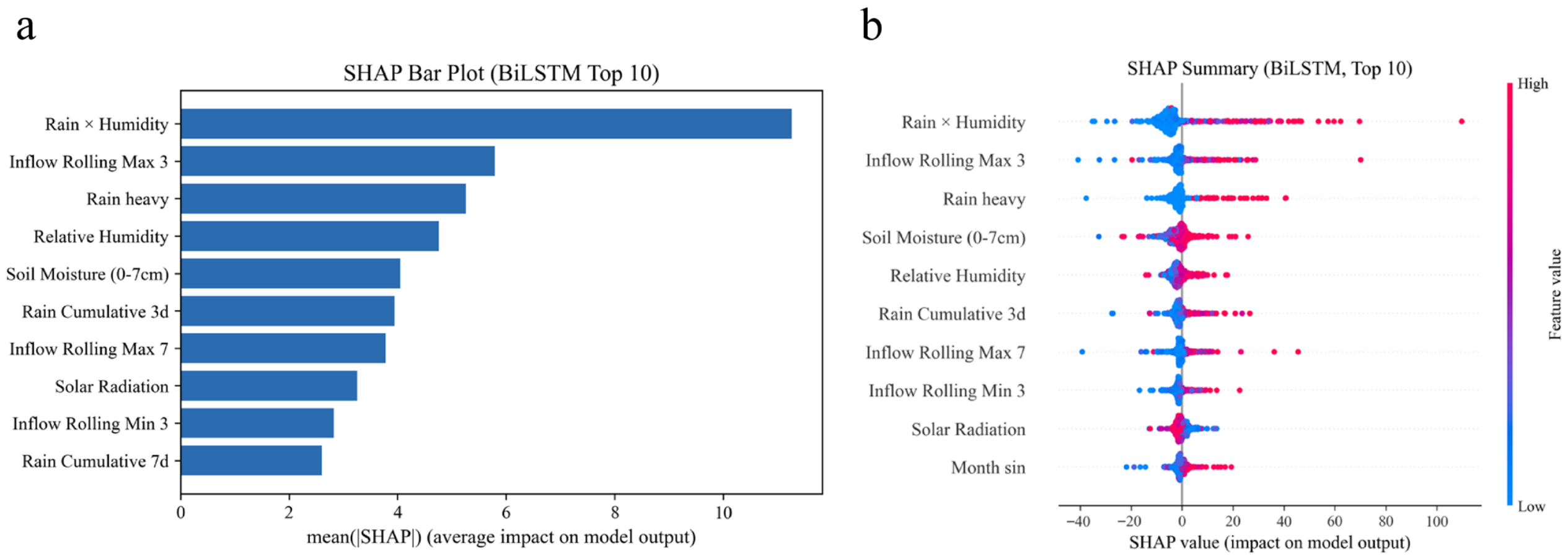The SHAP analysis of the BiLSTM model in Figure 10 indicates that the interaction terms of rainfall x soil moisture, cumulative rainfall, and short-term runoff extremes positively influence runoff prediction, aligning with the established hydrological principle that intense rainfall is more likely to elicit significant runoff responses under saturated initial conditions [50]. The modulation effects of temperature, radiation, wind speed, and vegetation illustrate the influence of energy balance and subsurface processes on runoff generation, aligning with prior ecological hydrological research [51].

The deep learning ensemble hybrid framework developed in this study utilizes BiLSTM as its backbone and incorporates XGBoost for residual compensation. This approach demonstrates superior accuracy, stability, and statistical consistency in predicting daily runoff. Future research should consider conducting comparative experiments across watersheds with varying climate zones and surface conditions. Additionally, integrating more meteorological data and surface characteristics—such as evapotranspiration and vegetation indices—could further validate the framework’s robustness and transferability. This would provide more reliable technical support for flood risk assessment and water resource management.

6. Conclusions

This study takes a hydrological monitoring station upstream of the Andi Reservoir in Zhejiang Province, China, as its research object. By obtaining ERA5 meteorological data, this study predicts runoff and proposes a residual sequence prediction method based on a bidirectional long short-term memory network (BiLSTM) and XGBoost integrated model. The aim is to overcome the limitations of traditional single models in predicting daily runoff and improve the accuracy of the prediction model. The main conclusions are as follows:

(1)

As a single deep learning model, BiLSTM exhibits enhanced performance, with lower prediction errors than LSTM and GRU. This improvement highlights the advantages of bidirectional architecture in accurately reflecting the extensive temporal dependency of runoff, which is particularly vital for event-driven hydrological processes.

(2)

By introducing XGBoost as a residual-correction module, the BiLSTM–XGBoost hybrid framework further improves prediction accuracy and stability. Compared with a single BiLSTM model, the hybrid model greatly reduces prediction errors and achieves higher efficiency coefficients, indicating that residual correction is effective in reducing system bias and capturing high-frequency nonlinear fluctuations that are difficult for sequence models to learn directly.

(3)

The SHAP-based interpretability analysis indicates clear functional differences between the two modeling stages. The single BiLSTM model primarily depends on hydrologically meaningful predictors, including rainfall–soil moisture interactions, accumulated rainfall, and short-term runoff extremes. These factors highlight the enhanced runoff response to storm events under wet antecedent conditions. By contrast, the hybrid model assigns greater importance to the BiLSTM predictions, corresponding residuals, and recent runoff information. This suggests that the XGBoost component mainly learns the error characteristics of the first-stage model and applies targeted nonlinear corrections.

Overall, the proposed interpretable framework improves prediction accuracy while increasing model transparency and reliability, supporting its potential application in real-time runoff forecasting, reservoir inflow prediction, and early flood warning. Moreover, the reliance on routinely available data and the moderate model complexity make the framework readily transferable to other catchments with similar data conditions.