Surface-Water Wetness Regulates the Urban Heat Island: An Explainable GeoAI Framework for Blue–Green Cooling in Arid Riyadh, Saudi Arabia

Abstract

Wetlands and surface-water features regulate the thermal environment of cities through evaporative cooling, yet in arid metropolitan regions these hydrological buffers are scarce and rarely quantified against urban heat. Here, we link satellite-derived surface-water wetness to land surface temperature (LST) and urban heat island (UHI) intensity in Riyadh, Saudi Arabia, using an explainable Geospatial Artificial Intelligence (GeoAI) framework. We assembled 2000 cloud-masked Landsat 8/9 sample points for July 2014 and 2024 in Google Earth Engine and derived the Normalized Difference Vegetation Index (NDVI), the Normalized Difference Built-up Index (NDBI), and two surface-water indices, the Modified Normalized Difference Water Index (MNDWI) and the Normalized Difference Water Index (NDWI), together with LST, UHI, terrain and population. Surface-water wetness was the strongest cool-side correlate of thermal stress: MNDWI related negatively to LST (r = −0.48) and to UHI intensity (r = −0.53), stronger than either vegetation or built-up density (both p < 0.001). Each 0.1 increase in MNDWI corresponded to a 2.2 °C reduction in LST. Five machine-learning algorithms predicted LST with test R² of 0.71–0.76 and UHI with R² of 0.68–0.72, and SHapley Additive exPlanations (SHAPs) identified MNDWI as the single most important thermal driver, ahead of elevation and vegetation. Point-level LST rose by 1.99 °C between 2014 and 2024 (p < 0.001), while open surface water was absent from all 2000 samples, indicating a hydrological deficit in the city’s thermal regulation. These findings suggest that protecting and expanding blue–green features along corridors such as Wadi Hanifah offers a measurable cooling lever for arid-city climate adaptation.

1. Introduction

The rapid pace of global urbanization is one of the most urgent challenges for building sustainable energy systems and climate resilience in the 21st century. Cities account for about 64% of worldwide primary energy consumption and produce over 70% of energy-related carbon emissions [1,2], and their expansion is reshaping Earth’s thermal environment through UHIs, in which built-up districts remain consistently hotter than their rural surroundings [3,4]. Rising urban temperatures elevate cooling energy demand, reduce HVAC efficiency and place cascading stress on electricity grids [5,6]. These pressures are most severe in arid and semi-arid regions, where intense radiation, extensive impervious surfaces and sparse vegetation can raise building cooling energy use by 30–50% [7,8]. What makes dryland cities distinctive, however, is that their surface energy balance is moisture-limited: with little water available for evaporation, absorbed radiation is partitioned almost entirely into sensible heat, so the scarcity of surface water is itself a first-order driver of urban warming.

Surface water and wetland features moderate urban temperatures because open water and moist surfaces dissipate incoming energy through evaporation rather than sensible heating [9,10]. Remote sensing offers the only practical means of observing this hydrological cooling at the metropolitan scale: water and wetness indices such as MNDWI and NDWI, derived from the same multispectral imagery that yields NDVI, NDBI and LST, allow surface moisture, vegetation, built-up density and temperature to be measured coherently across entire cities [11,12]. Multi-temporal satellite archives extend these observations across decades, and complementary platforms broaden them further; Bakirci [13] showed that sensor-equipped UAVs can autonomously monitor urban environments in dense areas, reflecting a wider trend toward integrated satellite, drone and ground observation [14,15]. In humid and temperate cities, water indices are routinely used to map inundation and to quantify the cooling influence of lakes, rivers and wetlands on LST. In arid metropolitan regions, by contrast, surface water is intermittent and confined to ephemeral wadis and engineered blue–green corridors, and its role in moderating heat remains poorly quantified even though water is the scarcest and most contested resource in these environments.

A comprehensive understanding of how urban structure shapes the thermal environment is therefore crucial for energy-efficient planning and climate resilience [16,17], and it demands interdisciplinary integration across climatology, environmental science, energy engineering and urban planning [18,19], particularly as cities pursue climate-resilient, net-zero development [20,21]. Machine learning (ML) increasingly connects these observations to prediction and planning. The integration of AI with geospatial technologies, commonly termed GeoAI, enables monitoring, predictive modeling and optimization in support of climate-resilient urban systems [22,23], and ensemble learning has outperformed traditional methods in modeling the relationships among urban morphology, thermal patterns and energy use [24,25,26]. Explainable techniques make these models auditable; SHAPs (SHapley Additive exPlanations [27]), grounded in cooperative game theory, attribute a prediction to each input by averaging their marginal contribution over feature orderings, and contrast with traditional approaches, single-index correlation or threshold mapping and ordinary regression without spatial validation, which neither rank competing drivers nor guard against spatial optimism. Such attribution quantifies the contribution of each driver to predicted temperature, supporting zone-specific building codes and climate-responsive design [28,29]. Zonation and clustering approaches can translate thermal maps into planning units [30,31,32,33], yet their usefulness depends on first establishing which surface property actually governs the thermal field—greenness, built-up density, or moisture—a question that explainable models are well-suited to answer.

Despite this progress, three gaps persist. First, studies of dryland UHIs overwhelmingly emphasize vegetation and built-up indices, and surface-water wetness is rarely tested as a candidate thermal driver [34,35,36,37], even though thermal dynamics in arid regions differ fundamentally from those in temperate climates [38,39]. Second, machine-learning analyses are seldom validated in a spatially honest way: random cross-validation overstates transferability when neighboring samples share information [40], and safeguards against information leakage between thermal targets and thermally derived predictors are rarely made explicit. Third, whether wetness–temperature relationships persist as arid cities densify remains underexplored, limiting their value for long-term adaptation planning [41,42]. To the best of our knowledge, no study has quantified the relative importance of surface-water wetness, vegetation, and built-up density as controls on LST in an arid Gulf metropolis within an explainable, spatially validated framework. Riyadh, one of the fastest-growing metropolitan areas in the Middle East, is an instructive setting for closing these gaps. Summer temperatures often surpass 45 °C, annual rainfall remains below 100 mm, and extensive sprawl places the city alongside Phoenix, Dubai, Abu Dhabi, Kuwait City and Doha among the world’s arid megacities [43,44]. Air-conditioning consumes over 60% of building energy, and low-density urban form with limited vegetation intensifies the thermal stress common to arid cities [45,46]. The city also contains a rare hydrological asset: the Wadi Hanifah corridor, rehabilitated into a linear wetland-park system, demonstrates that engineered blue–green infrastructure is feasible in this climate. Yet the contribution of surface-water wetness to thermal regulation across the wider metropolis has never been measured against vegetation and built-up density within a single predictive framework.

This study aims to quantify the role of surface-water wetness in regulating urban thermal stress in an arid metropolis and to embed that relationship in an explainable, reproducible GeoAI workflow. Specifically, we (i) derive vegetation, built-up and two surface-water indices (MNDWI, NDWI) together with LST and UHI intensity from cloud-masked Landsat 8/9 imagery for 2014 and 2024; (ii) test the strength and direction of the relationship between surface-water wetness and thermal stress relative to vegetation and built-up density; (iii) train five machine-learning algorithms to predict LST and UHI with explicit safeguards against information leakage, evaluating generalization under both random and spatially blocked cross-validation; and (iv) attribute the model predictions using SHAP to identify the dominant thermal drivers. To the best of our knowledge, this is the first study in an arid Gulf metropolis to demonstrate that surface-water wetness is the leading remotely sensed predictor of LST, providing a quantitative basis for blue–green cooling and wetland-corridor planning.

2. Materials and Methods

2.1. Methodological Framework

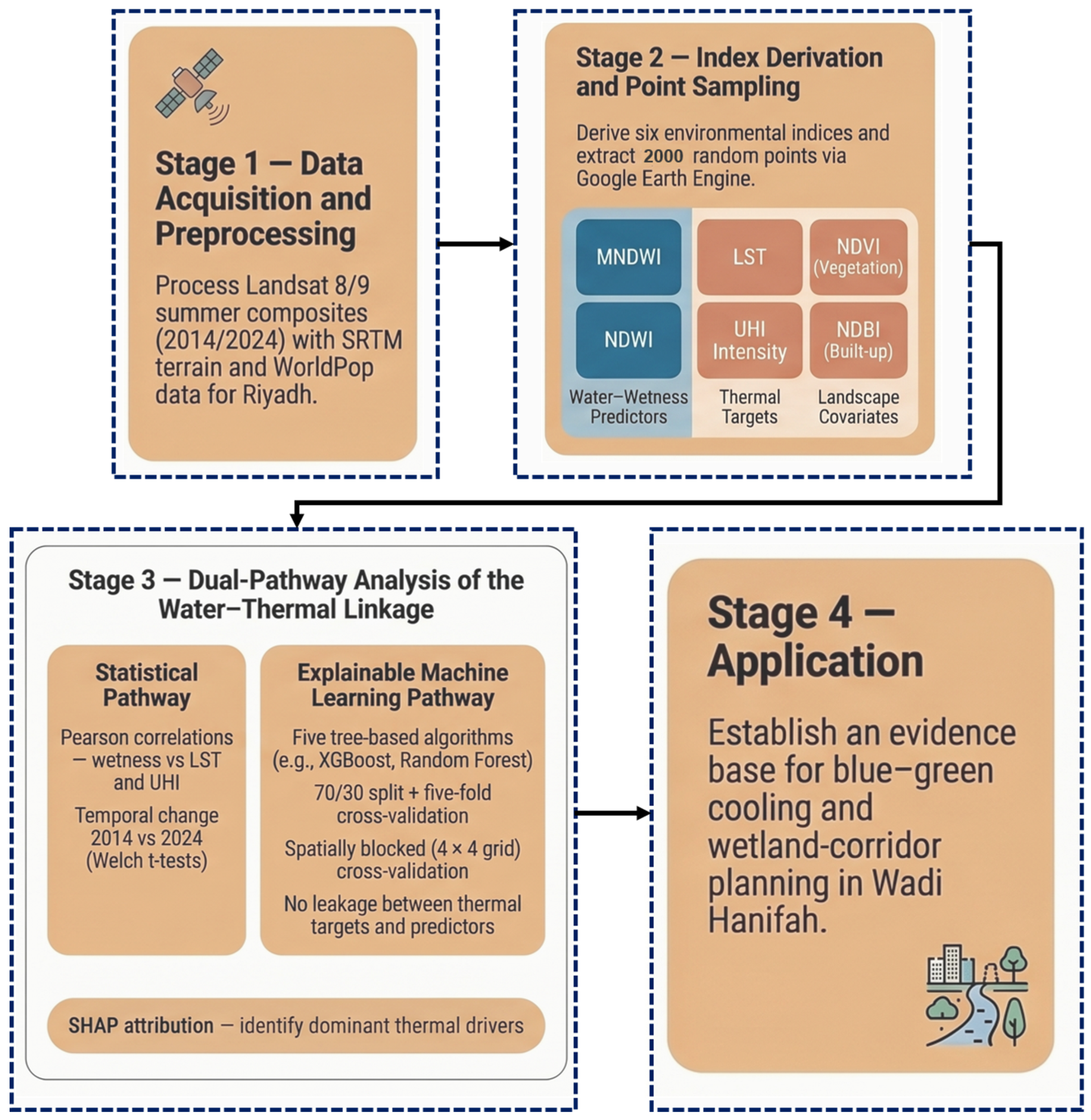
This study implements a four-stage analytical framework whose central purpose is to establish and quantify the linkage between surface-water wetness and urban thermal stress in an arid metropolis (Figure 1). In the first stage, cloud-masked Landsat 8/9 Collection 2 Level-2 imagery for peak summer 2014 and 2024 is assembled in Google Earth Engine together with SRTM terrain and WorldPop population data. The second stage derives the complete set of environmental indices, placing the water and wetness indices MNDWI and NDWI alongside NDVI, NDBI, LST and UHI intensity, and extracts all variables at 2000 random sample points so that surface moisture, vegetation, built-up density and temperature are measured coherently at the same locations. The third stage interrogates the water–thermal linkage along the following two parallel pathways: a statistical pathway that quantifies wetness–temperature relationships and their temporal change, and an explainable machine-learning pathway in which five algorithms predict LST and UHI under explicit leakage safeguards and both random and spatially blocked cross-validation, with SHAP attribution identifying the dominant thermal drivers. The final stage translates this evidence into blue–green cooling and wetland-corridor planning guidance for Riyadh and comparable arid cities.

2.2. Study Area Characteristics

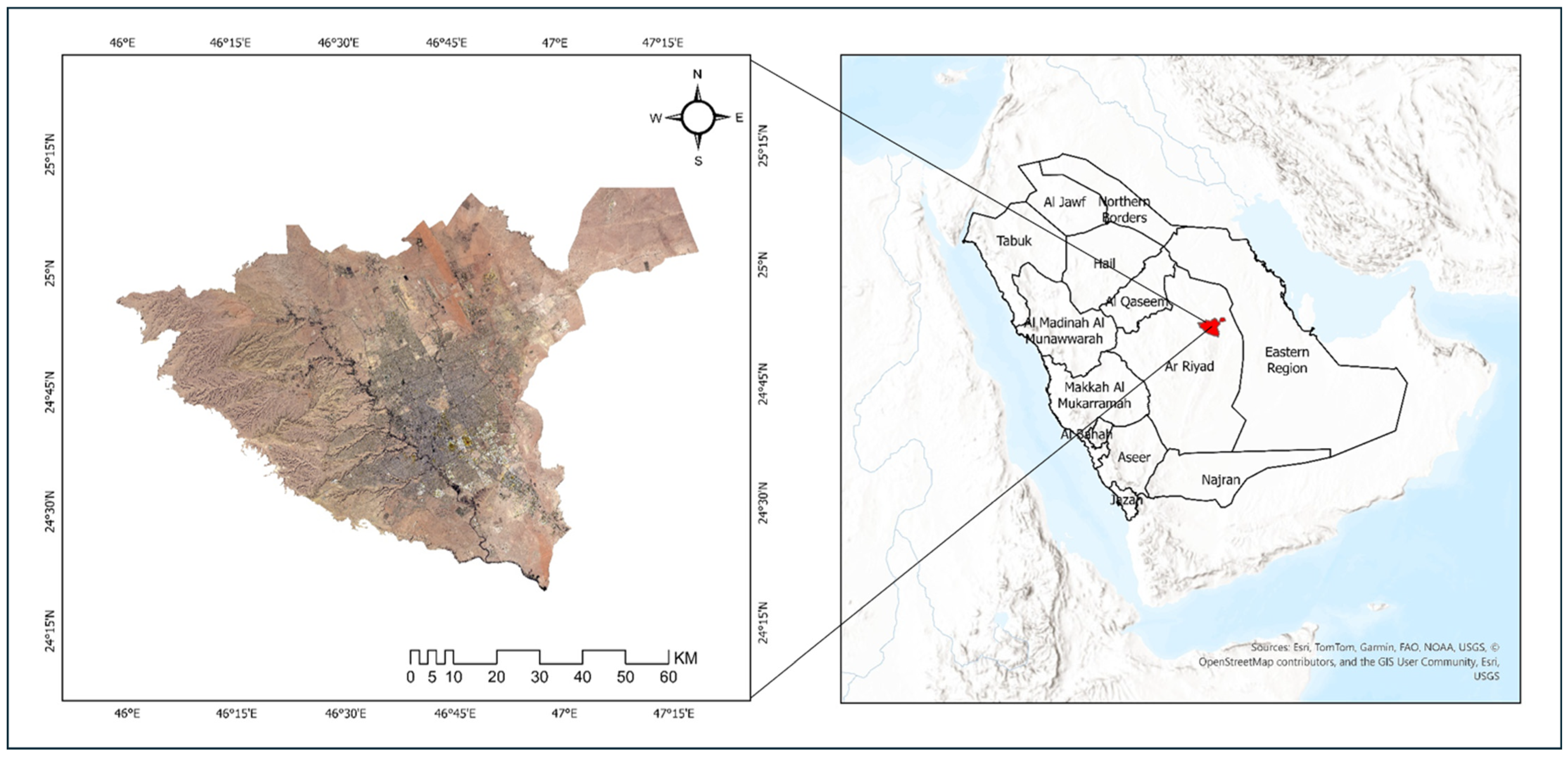
Riyadh, the capital of Saudi Arabia, is the focus of this GeoAI urban thermal analysis. It reflects rapid urban expansion patterns common in GCC cities, with increasing development, population, and environmental issues [47,48]. Located in central Saudi Arabia on the Najd Plateau at 24°15′–25°15′ N and 46°00′–47°15′ E, about 600 m above sea level, Riyadh features diverse geography. Wadi Hanifa passes through the west, while Wadi Al-Ha’ir lies in the south. The east is marked by Khashm Al-An, part of the Armah Mountain Range and Tuwaiq Mountain chain. According to the General Authority for Statistics, Riyadh’s current population is 7,009,120, a significant part of Saudi Arabia’s urban population, emphasizing the need to study urban thermal dynamics and building energy impacts [44]. The study area covers 5992.96 km² within Riyadh’s development boundaries, of which 51.98% (about 3115 km²) is urban, according to the Royal Commission for Riyadh City. The city has an arid climate with summer temperatures exceeding 45 °C, annual rainfall of less than 100 mm, and high solar radiation, leading to thermal stress that affects cooling loads and urban energy use [7,8]. Figure 2 shows the geographic location and extent of the study area for analysis.

2.3. Data Acquisition and Temporal Framework

This study used satellite images from Landsat 8 and 9, accessed through the USGS Earth Explorer platform (https://earthexplorer.usgs.gov). The details of these images are shown in

Table 1. Technical specifications of Landsat 8 and 9 satellite imagery used for temporal analysis (2014–2024).

Satellite Sensor	Path and Row	Spatial Accuracy	Date Acquired	Source
Landsat 8	165/043	30 m	24 July 2014	https://earthexplorer.usgs.gov
Landsat 8	166/043	30 m	31 July 2014
Landsat 9	165/043	30 m	24 July 2024
Landsat 9	166/043	30 m	31 July 2024

, explaining the technical aspects of the data collected for analyzing the period from 2014 to 2024. To keep things consistent, the study focused on imagery from July of both 2014 and 2024, aligning with the same season to ensure reliable thermal analysis. July was carefully chosen because it reflects the peak summer heat in Riyadh, when UHI effects are strongest, and building cooling needs are at their highest—perfect for planning energy use and HVAC systems [5,6]. Using the same month for both years helps avoid seasonal changes affecting the comparison, allowing us to see how urban growth over a decade has influenced thermal patterns more clearly [11]. Plus, the ten-year span from 2014 to 2024 captures significant urban expansion while staying relevant to current planning and development timelines [48].

While we acknowledge that single-month analysis may not fully capture year-round thermal dynamics or seasonal variations in UHI intensity, peak summer conditions remain the critical design scenario for cooling infrastructure and energy demand management in arid climates where extreme heat causes maximum building energy consumption [4,45]. The consistent patterns seen across both July datasets, along with the high model performance in temporal validation, indicate strong thermal-structural relationships during peak stress periods [37]. Future research will include multi-seasonal and annual data to explore seasonal UHI variability and verify the framework’s applicability throughout the year, focusing on a comprehensive temporal analysis of thermal-energy dynamics. The decade-long temporal span facilitates a comprehensive assessment of the impacts of urban transformation on thermal patterns, thereby supporting both retrospective analyses and predictive modeling applications pertinent to long-term energy infrastructure planning [41]. This period selection is consistent with established methodologies in urban thermal analysis, as the summer months offer optimal conditions for detecting the UHI owing to minimal rainfall, decreased cloud cover, and peak temperature readings [38,49].

2.4. Data Preprocessing and Quality Assurance

Data preprocessing adhered to rigorous protocols established in the recent remote sensing literature to guarantee data quality and analytical reliability [39,50]. Initial radiometric and geometric corrections were conducted using Erdas Imagine 2023 software, followed by systematic preprocessing of spectral bands to ensure data quality and consistency across both temporal datasets. The preprocessing workflow encompassed atmospheric correction to mitigate atmospheric interference effects, geometric rectification to ensure spatial accuracy and alignment between temporal datasets, and radiometric normalization to compensate for sensor differences between Landsat 8 and 9 platforms, thereby facilitating valid temporal comparisons [11,21].

Images from each study year were carefully combined through mosaicking to make sure the entire area was covered. This approach helped us account for the big changes in urban development and greenery over the decade-long period we studied [51]. Cloud masking techniques were used to remove any remaining cloud cover or atmospheric effects, ensuring our analysis was accurate and reliable. The cleaned and processed images then provided a solid foundation for both traditional remote sensing methods and innovative ML techniques. To ensure the highest data quality, we followed strict validation steps, including visual inspections, statistical checks, and verifying consistency across different parts of the analysis [50]. When handling missing data, we adhered to proven protocols, using spatial interpolation where needed and maintaining quality flags throughout the process.

2.5. Environmental Indices Calculation

The quantitative analysis of urban environmental conditions used four main indices, each with specific roles in describing urban thermal and vegetation patterns. The calculation method for these indices follows established procedures, with recent updates for better accuracy in arid urban areas [51,52].

NDVI is the key indicator for assessing vegetation cover and health across the study area [21]. The index is calculated using the standard formula shown in Equation (1):

NDVI = (NIR − RED)/(NIR + RED)

(1)

where NIR and RED are the reflectance values in the near-infrared and red spectral bands, respectively. NDVI values range from −1 to +1, with values near −1 indicating non-vegetative surfaces, values close to 0 representing sparse vegetation, and values near +1 signifying dense, healthy vegetation cover [50]. The interpretation scheme for NDVI is outlined in

Table 2. Classification schemes for the NDVI, NDBI, and UHI intensity indices. Class boundaries follow thresholds applied in previous arid-city studies [5,21].

Index	Value Range	Class
NDVI	<0	No vegetation
NDVI	0–0.05	Built-up area
NDVI	0–0.1	Very low vegetation
NDVI	0.1–0.2	Low vegetation
NDVI	>0.2	Moderate vegetation
NDBI	<0	No build-up
NDBI	0–0.05	Low build-up
NDBI	0.05–0.1	Dense build-up
NDBI	0.1–0.15	Arid area
NDBI	>0.15	Very arid area
UHI	<0	Low
UHI	0–0.05	Medium
UHI	0.05–0.1	High
UHI	0.1–0.15	Very high
UHI	>0.15	Extremely high

, providing standardized categories for vegetation density, from very low to very high.

The NDBI serves as a key indicator for detecting and measuring built-up areas based on the spectral features of impervious surfaces [39]. Its calculation uses the formula shown in Equation (2):

NDBI = (SWIR − NIR)/(SWIR + NIR)

(2)

where NIR and SWIR denote reflectance values in the near-infrared and shortwave-infrared spectral bands, respectively. NDBI values range from −1 to +1, with positive values indicating built-up areas and negative values signifying non-built-up areas, sparse development, water bodies, or vegetated regions [46]. Table 2 details the classification scheme for NDBI interpretation, allowing systematic categorization of urban density from very low to very high built-up intensity.

Complementing the vegetation and built-up indices, surface water and wetness were represented by two further indices computed from the green, near-infrared (NIR) and shortwave-infrared (SWIR1) bands of the Landsat 8/9 surface-reflectance product. The Modified Normalized Difference Water Index enhances open-water and moist surfaces while suppressing built-up signal, as defined in Equation (3) [9]:

MNDWI = (Green − SWIR1)/(Green + SWIR1)

(3)

NDWI, introduced by McFeeters [10], emphasizes the contrast between water and terrestrial surfaces, shown in Equation (4):

NDWI = (Green − NIR)/(Green + NIR)

(4)

Both indices range from −1 to +1; values approaching and exceeding zero denote increasing surface wetness or open water, whereas strongly negative values indicate dry, built-up or bare desert surfaces.

LST calculation is a vital component for understanding thermal interactions between the Earth and atmosphere. It also provides the basis for assessing UHI intensity [41,53]. The method uses thermal infrared bands (Band 10 for Landsat 8 and 9) following established procedures for Level 1 imagery processing. The LST calculation involves several steps carried out through systematic radiometric and thermal conversion algorithms [11].

Initially, Digital Number (DN) values are converted to Top of Atmosphere (TOA) spectral radiance (Lλ) using Equation (5):

Lλ = ML × Qcal + AL

(5)

where ML is the band-specific rescaling factor, AL is the band-specific additive rescaling factor, and Qcal are the thermal band DN values.

Next, TOA spectral radiance is converted to Top of Atmosphere Brightness Temperature (TC) using Equation (6):

TC = K₂/[ln(K1/L_λ + 1)] − 273.15

(6)

where K1 and K2 are thermal conversion constants specific to each band, and the temperature is converted from Kelvin to Celsius by subtracting 273.15.

Vegetation proportion (PV) is calculated using the relationship in Equation (7), which is crucial for determining surface vegetation proportions across the study area:

PV = [(NDVI − NDVI_min)/(NDVI_max − NDVI_min)]²

(7)

where NDVI_min and NDVI_max are the minimum and maximum NDVI values observed in the study area.

Thermal Emissivity (E) is calculated according to Equation (8), considering surface emissivity variations based on vegetation cover density:

E = 0.004 × PV + 0.986

(8)

Finally, LST is obtained using the comprehensive equation in Equation (9):

LST = TC/[1 + (λ × TC/ρ) × ln(E)]

(9)

where λ is the wavelength of emitted radiance (10.9 μm for Landsat 8/9 Band 10), and ρ = 1.438 × 10⁻² m·K, the second radiation constant of Planck’s law [11,51].

UHI intensity measures the temperature difference between urban areas and nearby rural regions, serving as a standard for evaluating thermal stress and building energy impacts [5,30]. The calculation uses the formula in Equation (10):

UHI = (Ts − Tm)/Tm

(10)

where Ts is the LST at a specific pixel, and Tm is the average LST across the entire study area. The UHI intensity thresholds are outlined in Table 2, which classifies thermal stress levels from low to extremely high. This classification supports applications like zone-specific building energy modeling and HVAC system optimization [32].

2.6. GeoAI Framework Implementation

2.6.1. Dataset Generation and Feature Engineering

Conventional remote-sensing outputs were transformed into a point dataset suitable for ML. From the cloud-masked composites, we drew 2000 spatially representative random sample points, evenly split between the two study years (1000 in 2014 and 1000 in 2024), and extracted every variable at each point at 30 m resolution. This balanced design supports temporally consistent model training and validation.

The predictors comprise the spectral indices (NDVI, NDBI, MNDWI and NDWI), terrain attributes (elevation, slope and aspect from the 30 m SRTM digital elevation model), gridded population density (WorldPop), the geometric distance of each point from the city center, and the acquisition year. LST and UHI intensity were treated solely as prediction targets and were never supplied as predictors of one another, nor of the thermal-stress class derived from them, which removes information leakage by construction.

The point dataset supports the following three modeling targets reported here: regression of LST, regression of UHI intensity, and a UHI thermal-stress classification in which the class-defining UHI value is excluded from the predictors (

Table 3. Predictor sets for each modeling target, confirming that no target or target-derived variable entered its own predictor set.

Predictive Target	Predictors Supplied	Variables Excluded
LST (regression)	NDVI, NDBI, MNDWI, NDWI, elevation, slope, aspect, population density, distance from center, year	LST, UHI
UHI intensity (regression)	NDVI, NDBI, MNDWI, NDWI, elevation, slope, aspect, population density, distance from center, year	LST, UHI
UHI thermal-stress class	NDVI, NDBI, MNDWI, NDWI, elevation, slope, aspect, population density, distance from center, year	LST, UHI and the class-defining UHI value

).

2.6.2. ML Algorithm Selection and Implementation

We trained the following five tree-based ensemble algorithms that are well-established for non-linear environmental prediction: Random Forest, Extremely Randomized Trees (Extra Trees), Gradient Boosting, Histogram-based Gradient Boosting and XGBoost. These complementary bagging and boosting methods capture non-linear relationships among the spectral, terrain and population predictors without assuming a functional form, and were implemented in Python 3.14 (scikit-learn and XGBoost). Their hyperparameters are listed in

Table 4. Hyperparameters of the five ensemble algorithms; all used a 70/30 train-test split with five-fold cross-validation.

Algorithm	Key Hyperparameters
Random Forest	150 trees; default depth; bootstrap; random_state = 42
Extra Trees	150 trees; default depth; random_state = 42
Gradient Boosting	100 estimators; learning rate 0.1; max depth 3; random_state = 42
Histogram Gradient Boosting	max iterations 100 (default); random_state = 42
XGBoost	250 trees; max depth 4; learning rate 0.06; subsample 0.8; colsample_bytree 0.8; random_state = 42

.

2.6.3. Explainable ML and Validation Protocol

Predictive performance was assessed on a 70/30 train-test split and confirmed with five-fold cross-validation, reporting the coefficient of determination (R2), root-mean-square error (RMSE) and mean absolute error (MAE) on the held-out set. To evaluate spatial generalization rather than mere interpolation, models were additionally tested with spatially blocked cross-validation, in which the study area was partitioned into a 4 × 4 grid of contiguous blocks so that test samples were always spatially disjoint from training samples; sensitivity to 3 × 3 and 5 × 5 grids was also examined. Model predictions were attributed using SHAP (SHapley Additive exPlanations), a game-theoretic method that assigns each feature its average marginal contribution to a prediction, preferred here over single-tree or permutation importance because it is locally consistent and model-agnostic.

2.7. Spatial Clustering Analysis

2.7.1. Clustering Algorithm Selection and Implementation

Spatial clustering grouped the 2000 sample points into thermal-environmental zones from their standardized values of the following six variables: NDVI, NDBI, MNDWI, NDWI, LST, and UHI intensity. K-means was used as the primary algorithm and DBSCAN as a density-based check for irregular structure and noise.

2.7.2. Optimal Cluster Determination and Validation

The number of zones was selected using three internal validity criteria evaluated for k = 2 to 8: the silhouette coefficient (cluster cohesion versus separation), the Davies–Bouldin index (lower values indicate better separation) and the Calinski–Harabasz index. The solution that maximized the silhouette coefficient was retained as optimal.

2.7.3. Cluster Characterization

The retained zones were first mapped in geographic and feature spaces and then characterized by the mean of each variable, yielding an interpretable description of each thermal-environmental zone prior to any planning interpretation.

This characterization supports blue-green planning by distinguishing hotter, drier districts, which are priority targets for moisture-led cooling, from cooler, moister districts where the marginal cooling benefit is smaller.

2.8. Statistical Analysis and Integration

Statistical analysis comprised five components, all implemented in Python (scikit-learn, XGBoost, SHAP and statsmodels). First, Pearson correlation coefficients quantified bivariate relationships among the indices and thermal variables. Second, temporal differences between 2014 and 2024 were tested with Welch’s t-test, chosen because it does not assume equal variances between the two yearly samples; the conclusions were unchanged under the non-parametric Mann–Whitney U test. Third, because the four spectral indices are built from overlapping spectral bands and are therefore collinear, we computed variance inflation factors (VIFs) and the condition index and supported the bivariate findings with partial correlations (controlling for NDVI and NDBI) and a reduced multivariable regression in which collinearity was acceptable (all VIF below 9). Fourth, the slope of LST on MNDWI was estimated by ordinary least squares with 95% confidence intervals and re-estimated separately by year and by spatial block. Fifth, to translate the wetness signal into corridor-design terms, the distance of each sample point to the Wadi Hanifah corridor (approximated from its mapped course) was computed, and LST, UHI and MNDWI were summarized across distance bands.

2.9. Point Sampling and Data Integration in Google Earth Engine

Image processing and sampling were implemented in Google Earth Engine. For each epoch (July 2014 and July 2024) we filtered Landsat 8 (and Landsat 9 from 2022) Collection 2 Level-2 scenes over the study-area bounding box (24°15′–25°15′ N, 46°00′–47°15′ E), masked cloud, cloud-shadow, cirrus and dilated-cloud pixels using the QA_PIXEL band, applied the Collection 2 scaling factors, and reduced the collection to a median composite. From each composite, we computed NDVI, NDBI, MNDWI, NDWI, and LST. LST was taken from the atmospherically corrected Collection 2 Level-2 surface-temperature band and converted to degrees Celsius; UHI intensity was derived from LST following Equation (10). We added terrain attributes (elevation, slope and aspect from the 30 m SRTM digital elevation model), gridded population (WorldPop, 100 m), and the geometric distance of each point from the city center. We then drew 1000 random sample points per epoch (2000 in total) and extracted all variables at 30 m resolution. Because the WorldPop 100 m series ends in 2020, the 2024 points use the 2020 population layer; this is noted as a limitation. The following two complementary LST pathways underlie the paper: the emissivity-based retrieval of Equations (5)–(9) supports the LST maps, whereas the point dataset uses the Collection 2 Level-2 surface-temperature product; both derive from the thermal band acquired at 100 m and distributed resampled to 30 m, and all point extractions were performed at 30 m.

3. Results

3.1. Spatiotemporal Analysis of Vegetation Cover Dynamics

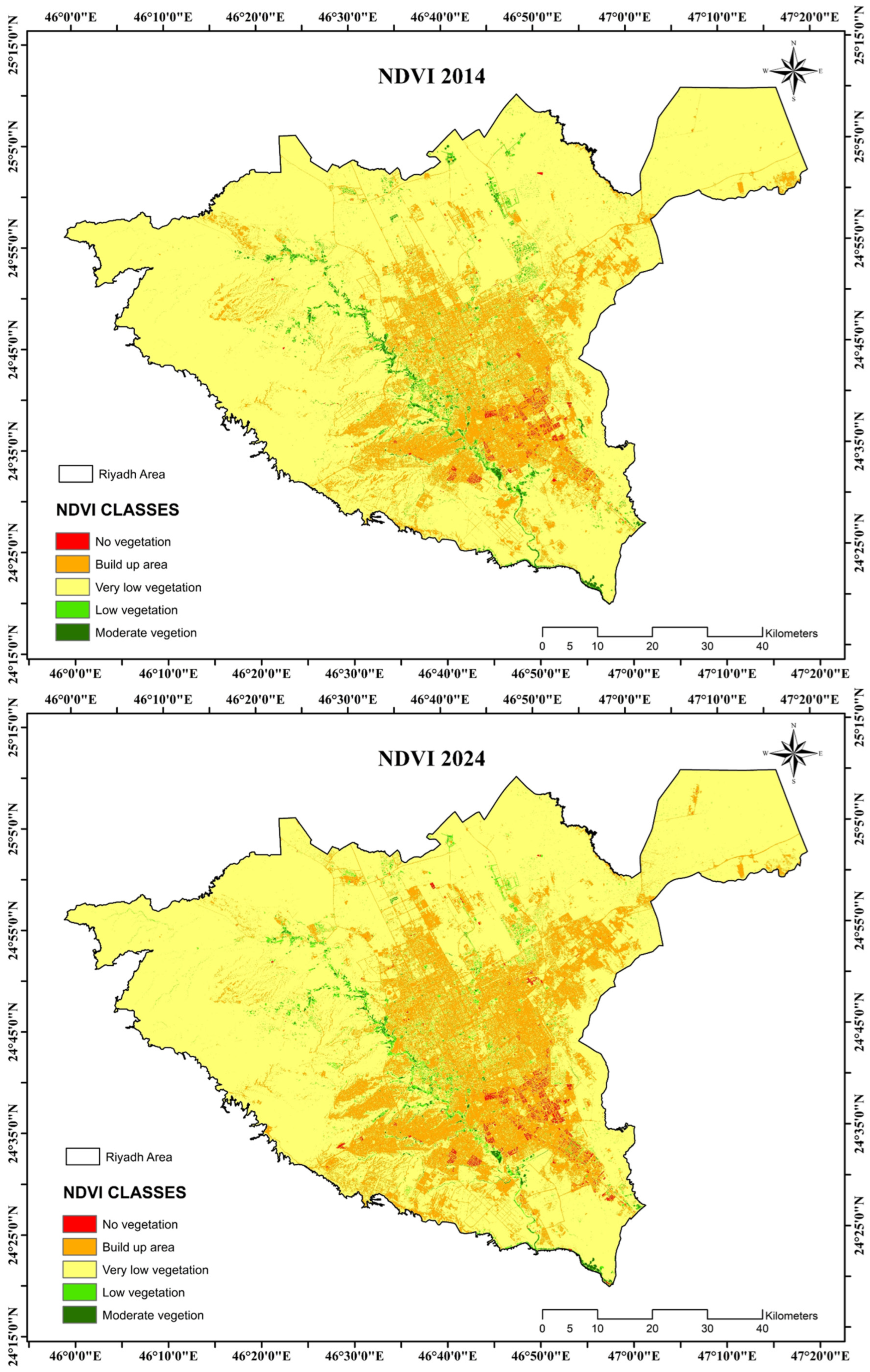
The NDVI analysis demonstrated significant changes in vegetation distribution across Riyadh over the study period, as depicted in Figure 3. The comprehensive evaluation of vegetation patterns indicates notable changes in land-cover composition from 2014 to 2024. Non-vegetated and built-up areas accounted for 0.42% and 15.97% of the total area in 2014, respectively, increasing to 0.61% and 20.57% by 2024. This expansion reflects an increase of 287.38 km² in built-up regions over the ten-year study period.

The analysis indicates that vegetation cover classified as very low, which predominantly characterized the landscape under examination, diminished from 81.01% in 2014 to 76.43% in 2024. This trend reflects a systematic reduction in sparse vegetation throughout the metropolitan region. Conversely, areas characterized by low vegetation cover decreased from 2.02% to 1.91%, while regions with moderate vegetation experienced a more notable decline from 0.59% to 0.48% of the total area studied, as delineated in

Table 5. Land-cover composition change in Riyadh between 2014 and 2024, derived from NDVI and NDBI classification.

Indicator	Class	2014 (%)	2024 (%)
Vegetation (NDVI)	No vegetation	0.42	0.61
Vegetation (NDVI)	Built-up	15.97	20.57
Vegetation (NDVI)	Very low vegetation	81.01	76.43
Vegetation (NDVI)	Low vegetation	2.02	1.91
Vegetation (NDVI)	Medium vegetation	0.59	0.48
Built-up (NDBI)	No build-up	4.51	3.47
Built-up (NDBI)	Build-up surface	14.75	20.15
Built-up (NDBI)	Arid area	78.21	72.50
Built-up (NDBI)	Sand dunes	2.54	3.88

. These observations indicate an overall reduction in vegetation cover across all density categories, with medium-density vegetation showing the most significant relative decrease of 18.64%. Vegetation loss varied across the study area, with the northeastern and southeastern sectors experiencing the most reduction due to urban development. In contrast, areas along Wadi Hanifa and natural corridors remained relatively stable, serving as green infrastructure within the expanding city.

3.2. Urban Development Pattern Analysis

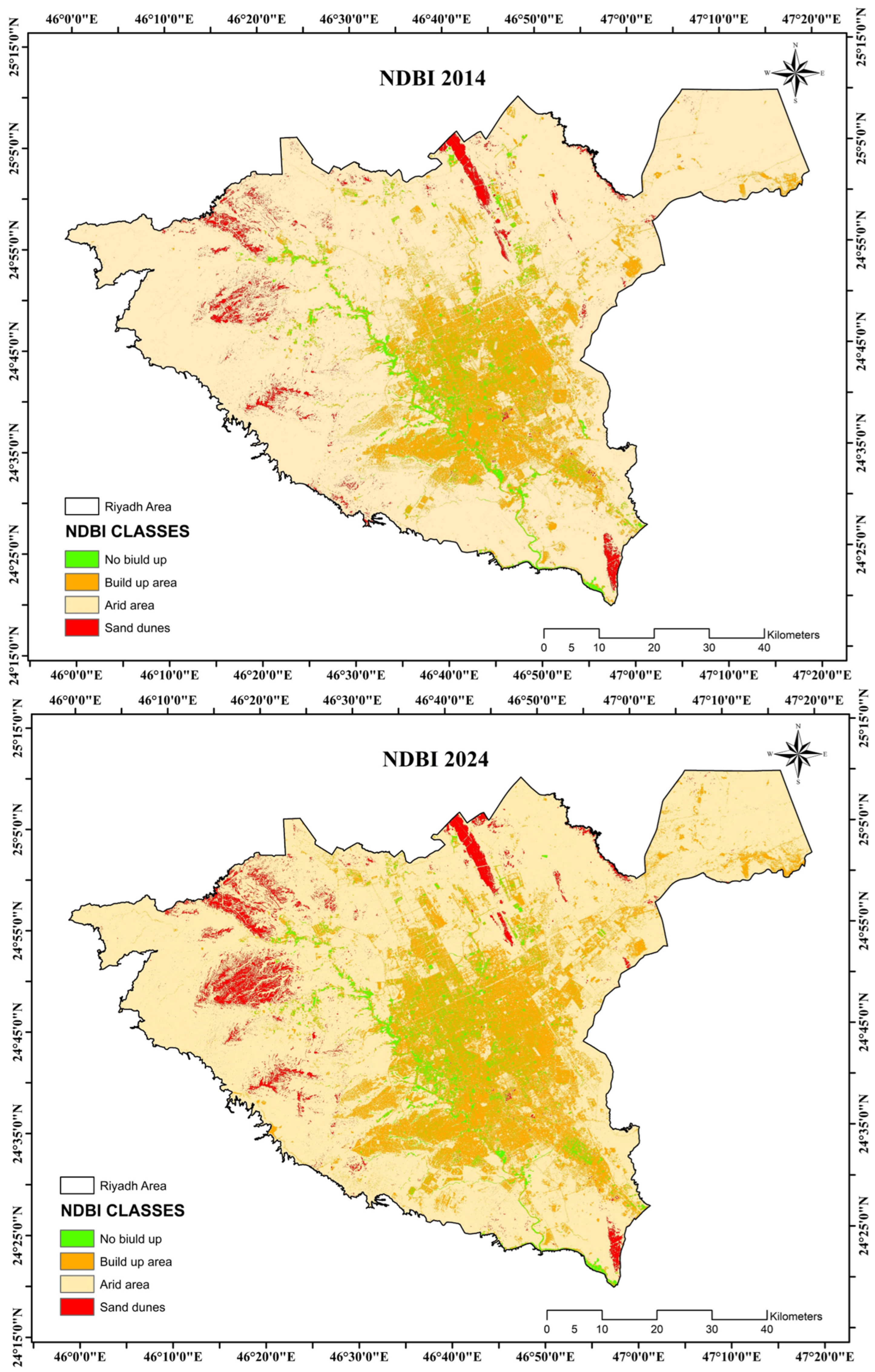
The NDBI analysis revealed significant urban growth from 2014 to 2024, as shown in Figure 4. Built-up areas grew substantially from 14.75% to 20.15% of the total study area, adding 323.56 km² of new urban land. This growth mainly came at the expense of arid regions, which shrank from 78.21% to 72.50%, reflecting a systematic conversion of undeveloped land to urban use. The NDBI-derived build-up surface (14.75% to 20.15%) differs slightly from the NDVI-derived built-up class (15.97% to 20.57%, Section 3.1) because the two indices define built-up land by different spectral criteria; both indicate the same ~5 percentage-point expansion.

Non-built-up areas, mainly consisting of vegetated regions and open spaces, decreased from 4.51% to 3.47% of the study area, which is roughly a 62 km² reduction. The spatial patterns showed that urban growth expanded outward from the existing urban core in a radial manner, with notable growth along major transportation routes and infrastructure networks.

Table 5 provides a comprehensive quantification of these urban development modifications, showing that the area of sand dunes increased from 2.54% to 3.88%. This increase potentially reflects land preparation activities and construction-related disturbances within expansion zones. The analysis indicates that urban growth was characterized by medium- to high-density development patterns rather than low-density sprawl, thereby implying the adoption of concentrated urbanization strategies. The small difference between the NDVI-derived built-up share (20.57%) and the NDBI-derived built-up surface (20.15%) reflects the different spectral definitions of the two indices rather than an inconsistency.

3.3. Temporal Change Detection Analysis

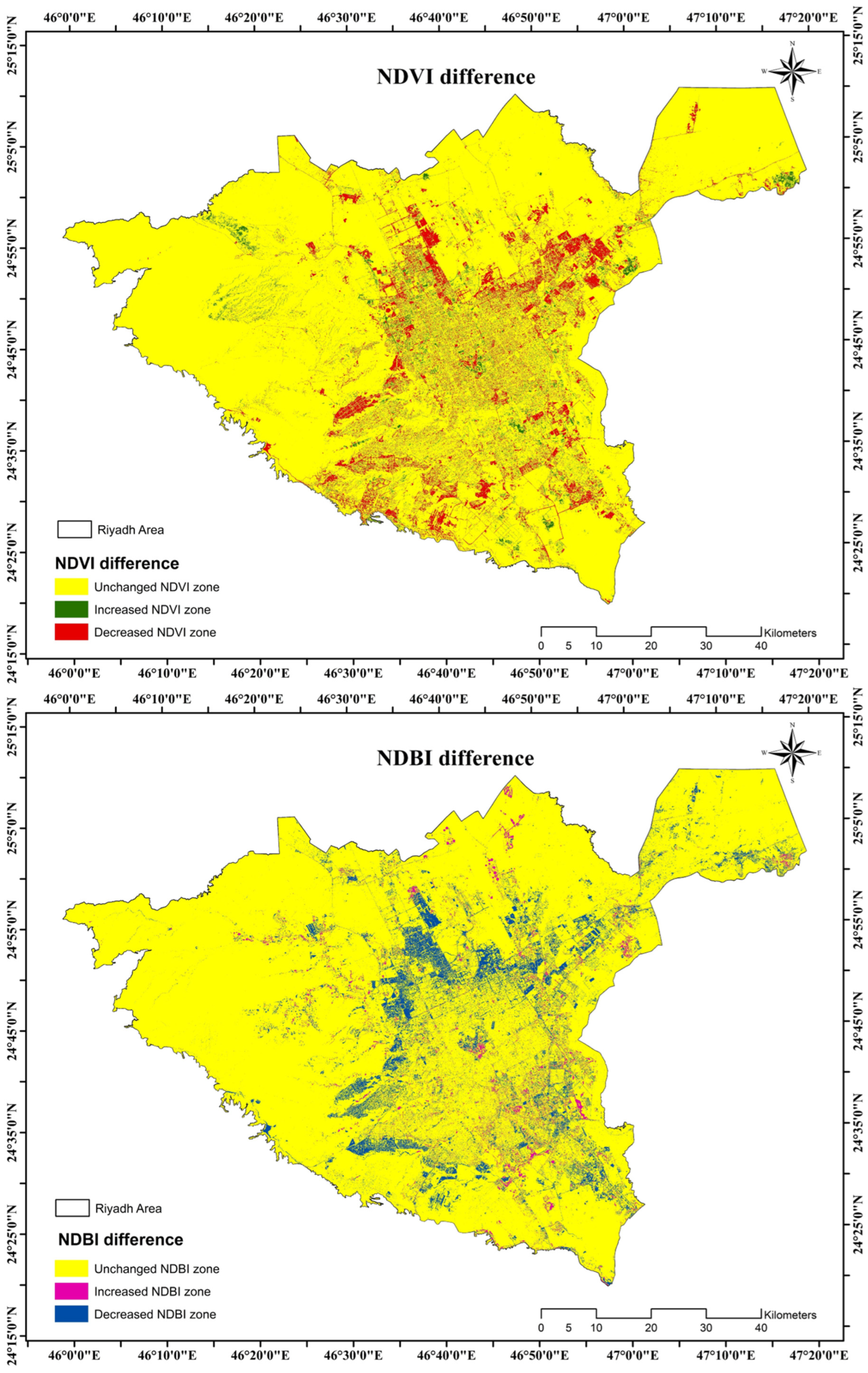
The analysis of NDVI and NDBI variations from 2014 to 2024 indicates urban expansion and vegetation reduction, as depicted in Figure 5. Difference maps show that 2.45% of the territory experienced an increase in NDBI, while 8.58% experienced decreases, reflecting complex urban development and renewal processes. Likewise, NDVI variations revealed that 3.37% of the area showed an increase in vegetation index values, while 8.42% showed declines. Regions with no alterations in either index, accounting for 88.96% for NDBI and 88.20% for NDVI, predominantly correspond to non-urbanized zones distant from the city center and established urban sectors with consistent land use patterns. Table 5 quantifies these temporal changes, showing that areas of NDVI decrease (504.62 km²) substantially exceeded areas of increase (202.36 km²), leading to a net vegetation loss of 302.26 km² over the study period. The spatial distribution of changes reveals that vegetation gains mainly occurred in planned green space developments and urban landscaping projects, while declines were mostly found in urban expansion zones and areas of infrastructure growth. Because these areas derive from single-composite classifications, values reported to fractions of a square kilometer should be read as indicative central estimates rather than exact measurements.

3.4. LST Pattern Analysis

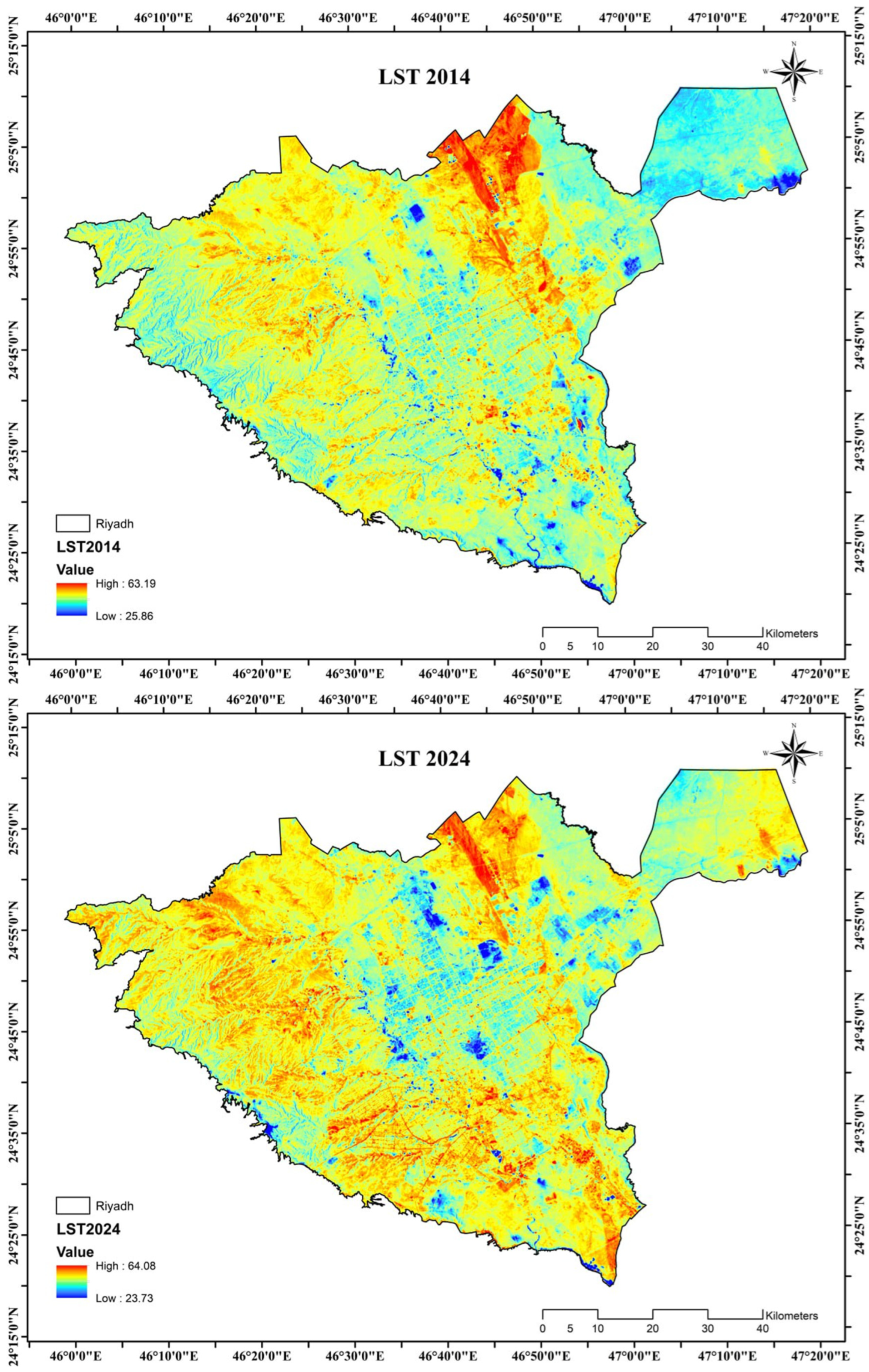
The LST analysis uncovered notable thermal fluctuations and temporal variations throughout the study period, as illustrated in Figure 6. LST values ranged from 25.86 °C to 63.19 °C in 2014 and expanded to a range of 23.73 °C to 64.08 °C in 2024, indicating both cooling in certain areas and an escalation of maximum temperatures. The spatial distribution patterns demonstrate that the highest temperatures were consistently observed in desert and arid regions surrounding the urban environment, whereas urban green spaces and vegetated areas exhibited markedly lower temperatures. The temporal comparison shows systematic increases in surface temperatures across urban zones, with the most significant changes occurring in newly developed sectors and regions experiencing vegetation reduction. The maps depict distinct thermal gradients emanating from the urban core, with temperature disparities of up to 15–20 °C between vegetated zones and built-up areas during peak summer conditions. Zones of intensive urban development, particularly commercial and industrial regions, continuously displayed elevated surface temperatures surpassing 55 °C during the summer peak. Conversely, established parks, green corridors, and areas with extensive tree cover maintained temperatures 8–12 °C lower than adjacent built-up zones, thereby illustrating the considerable cooling influence of urban greenery.

3.5. UHI Intensity Assessment

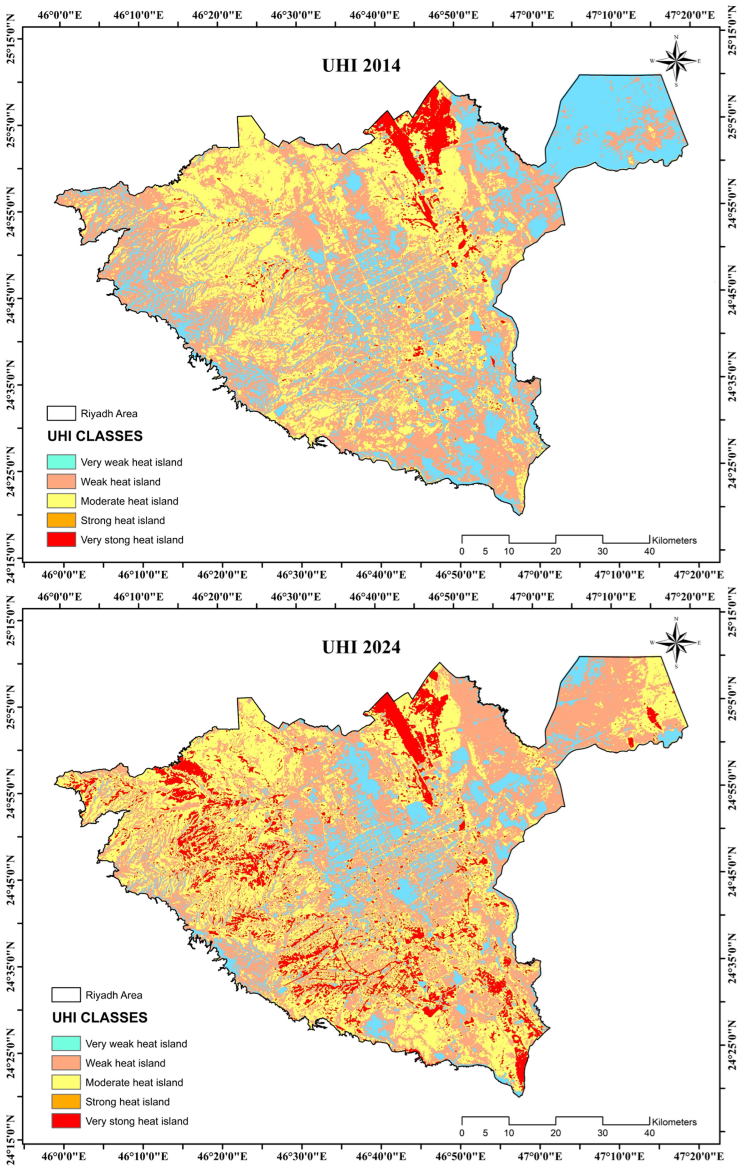
The UHI analysis shows notable changes in thermal stress from 2014 to 2024, as detailed in Figure 7. Areas with high UHI intensity grew from 39.05% to 43.08%, reflecting a wider spread of thermal stress across the city. More strikingly, very high UHI regions expanded from 13.70% to 32.49%, and extremely high UHI areas increased from 1.98% to 5.24%. A concerning trend is the sharp decline in low UHI zones, dropping from 9.04% to 2.61%, which means a reduction of 385.61 km² of these areas. This indicates a systematic intensification of urban heat stress in the metropolitan region. The quantification of these changes highlights the growing degradation of the thermal environment. Furthermore, areas with medium UHI intensity saw a significant decrease from 36.24% to 16.58%, covering a loss of 1178.00 km². Along with the growth of high and very high UHI zones, this suggests a clear shift toward more severe thermal conditions throughout Riyadh. The spatial patterns reveal that UHI intensification was particularly concentrated in zones with dense urban development, less vegetation, and more impervious surfaces. Specifically, areas along major transportation routes and commercial districts experienced the most intense increases in UHI. These five classes (low, medium, high, very high and extremely high) follow the thresholds in Table 2 and the legend of Figure 7.

3.6. LST and UHI Change Pattern Analysis

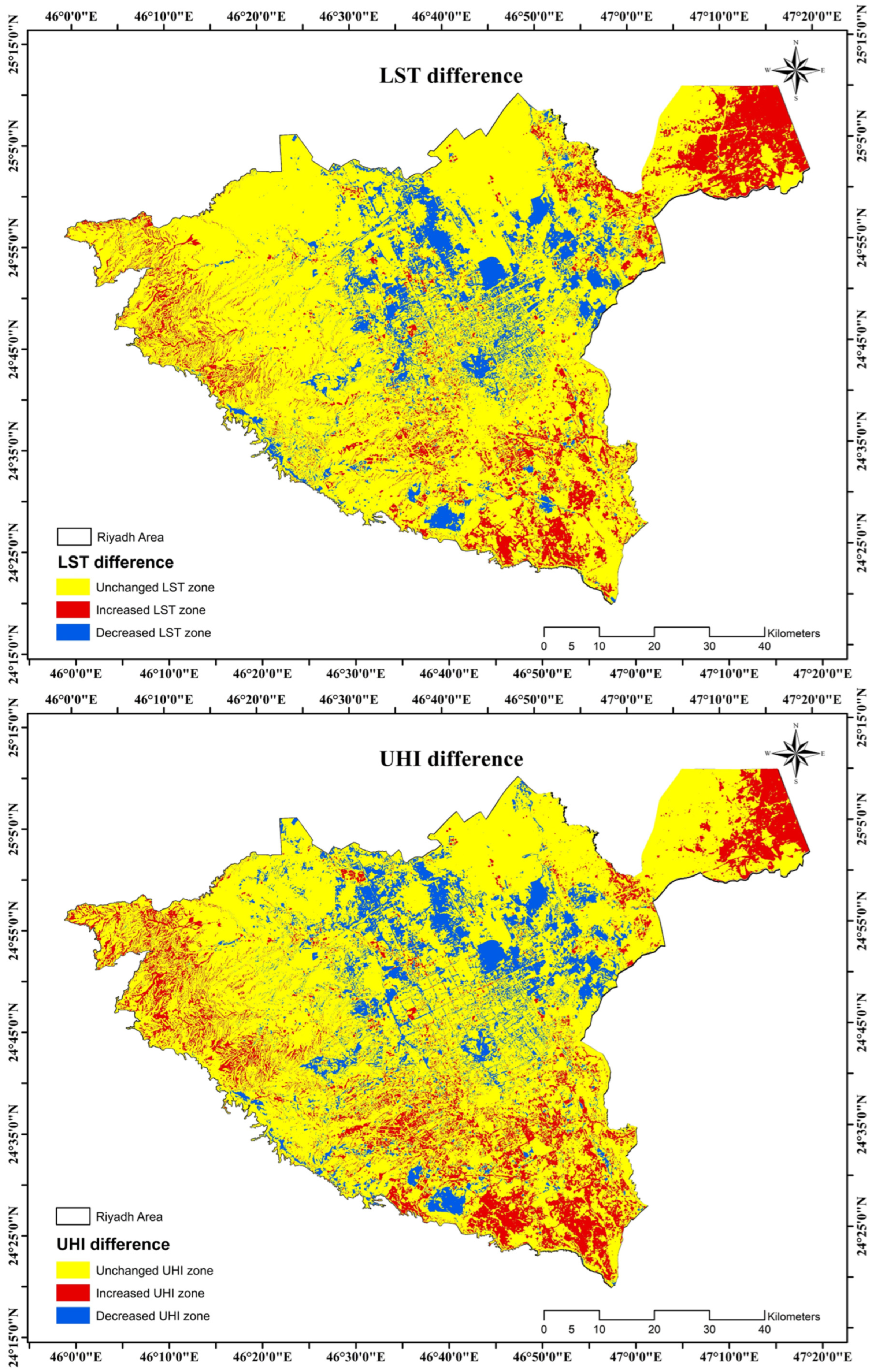
The comprehensive difference analysis between 2014 and 2024 revealed significant spatial patterns in both LST and UHI changes, as shown in Figure 8. The northeastern and southeastern parts of the study area showed the largest increases in LST, aligning with areas of intense urban development and vegetation loss identified earlier. The spatial relationship between LST and UHI changes indicates a strong link between surface temperature shifts and heat island intensity variations. Areas with LST increases of 3–8 °C generally corresponded to UHI intensity increases of 0.05–0.15 units, demonstrating systematic connections between surface thermal properties and UHI formation.

Table 5 details these changes, indicating that 13.25% of the study area (794.28 km²) experienced increases in LST, while 10.38% (621.83 km²) saw decreases. The UHI index showed similar trends, with 14.62% of the area (875.99 km²) exhibiting higher intensity and 11.46% (686.97 km²) showing decreases. The areas that remained unchanged, representing 76.37% for LST and 73.92% for UHI, mostly corresponded to stable urban zones and undeveloped regions far from expansion corridors. Nonetheless, even within these stable zones, subtle shifts in thermal patterns were detected, indicating that urban heat island effects extend beyond immediate development areas.

3.7. Surface-Water Wetness as the Dominant Cooling Signal

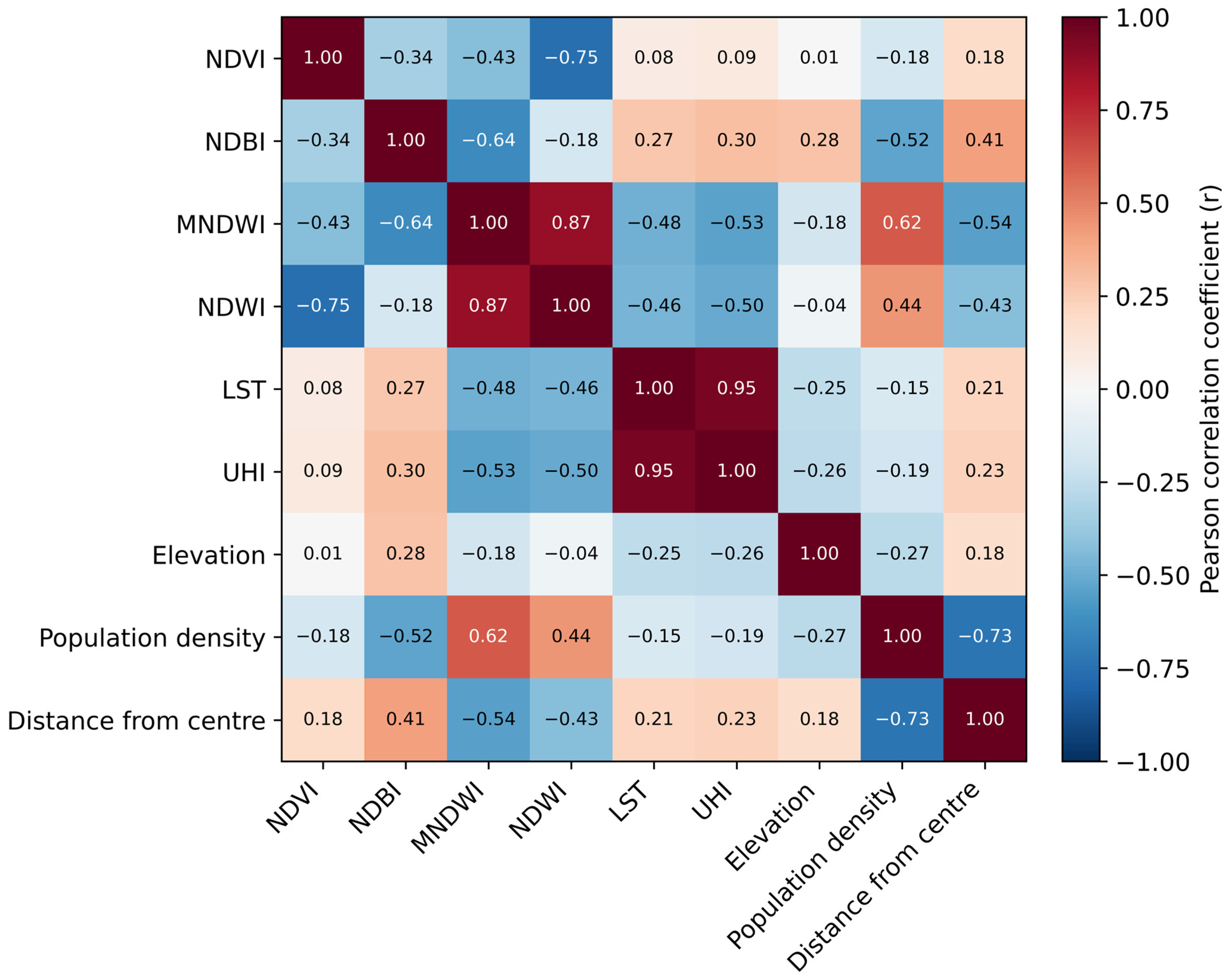
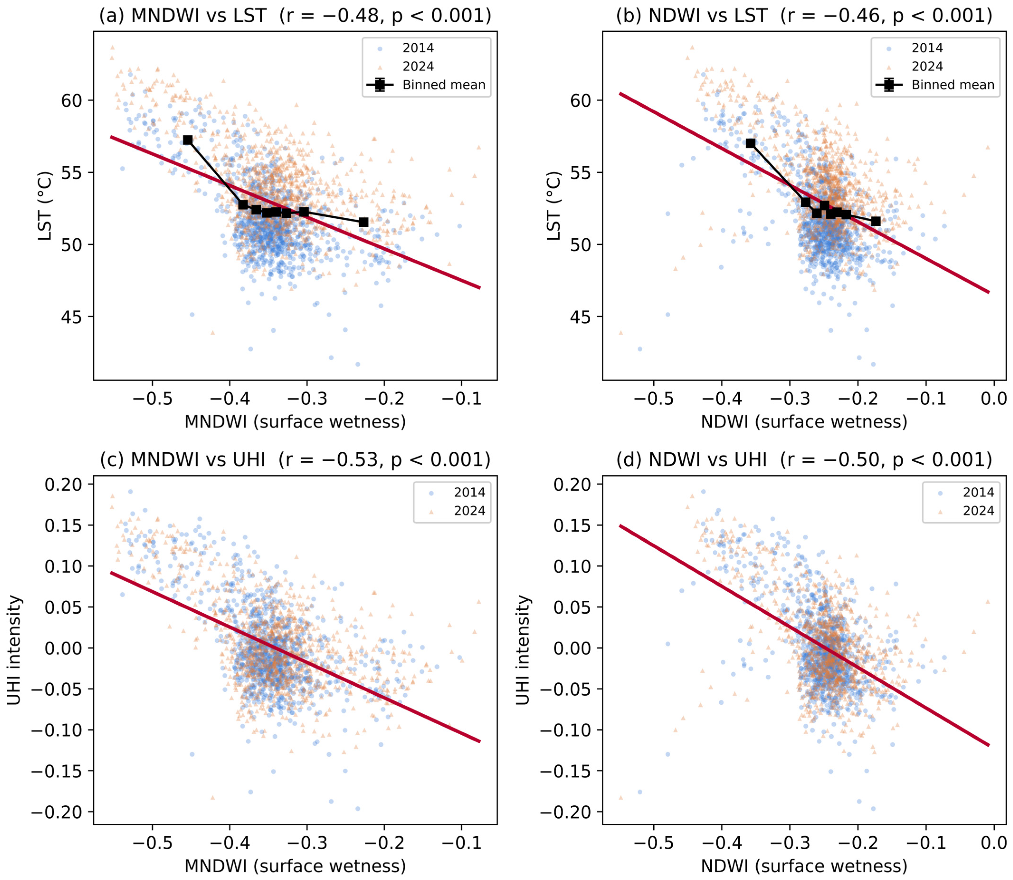
Surface-water wetness was the strongest cool-side correlate of thermal stress across the 2000 sample points. MNDWI related negatively to LST (r = −0.48, p < 0.001) and to UHI intensity (r = −0.53, p < 0.001), and NDWI showed the same pattern (r = −0.46 and −0.51, respectively). These wetness–temperature relationships were stronger than the warming effect of built-up density (NDBI–LST r = 0.27) and far exceeded the weak vegetation signal (NDVI–LST r = 0.08), indicating that, in this arid setting, moisture availability rather than greenness governs the surface thermal field (Figure 9 and Figure 10). The relationship was practically meaningful: each 0.1 increase in MNDWI corresponded to a 2.2 °C reduction in LST, and each 0.1 increase in NDWI to a 2.5 °C reduction (

Table 6. Relationships between surface-water and vegetation indices and thermal stress (LST, UHI intensity).

Index	Target	Pearson r	p	Slope	Change Per +0.1
MNDWI	LST	−0.483	<0.001	−21.919	−2.192
MNDWI	UHI intensity	−0.534	<0.001	−0.432	−0.043
NDWI	LST	−0.462	<0.001	−25.447	−2.545
NDWI	UHI intensity	−0.505	<0.001	−0.496	−0.05
NDVI	LST	0.082	<0.001	6.973	0.697
NDVI	UHI intensity	0.095	<0.001	0.144	0.014
NDBI	LST	0.267	<0.001	21.151	2.115
NDBI	UHI intensity	0.302	<0.001	0.426	0.043

). Notably, open surface water (MNDWI > 0) was absent from all 2000 samples, so the cooling gradient operated entirely within the moist-to-dry range of an essentially waterless surface.

The temporal comparison reinforced an intensifying thermal regime. Mean point-level LST rose from 51.85 °C in 2014 to 53.85 °C in 2024, a significant increase of 1.99 °C (p < 0.001), while the built-up index declined marginally and mean wetness changed little (

Table 7. Descriptive statistics of the sampled variables by year (n = 1000 per year).

Variable	Mean 2014	SD 2014	Mean 2024	SD 2024	Change	p
NDVI	0.1	0.034	0.098	0.036	−0.002	0.319
NDBI	0.105	0.036	0.101	0.039	−0.004	0.011
MNDWI	−0.348	0.059	−0.34	0.071	0.008	0.004
NDWI	−0.253	0.049	−0.248	0.058	0.005	0.054
LST (°C)	51.852	2.725	53.846	2.844	1.995	<0.001
UHI intensity	0.000	0.053	0.003	0.053	0.003	0.177
Elevation (m)	678.013	100.952	673.588	100.433	−4.425	0.326
Population density	3.12	5.461	4.403	7.277	1.283	<0.001
Distance from center (m)	45,610.544	17,228.079	45,136.47	17,914.469	−474.073	0.546

). The persistence of strongly negative wetness values in both epochs, alongside rising temperatures, shows that the surface offered little additional evaporative relief over the decade.

3.8. Explainable GeoAI of Thermal Drivers

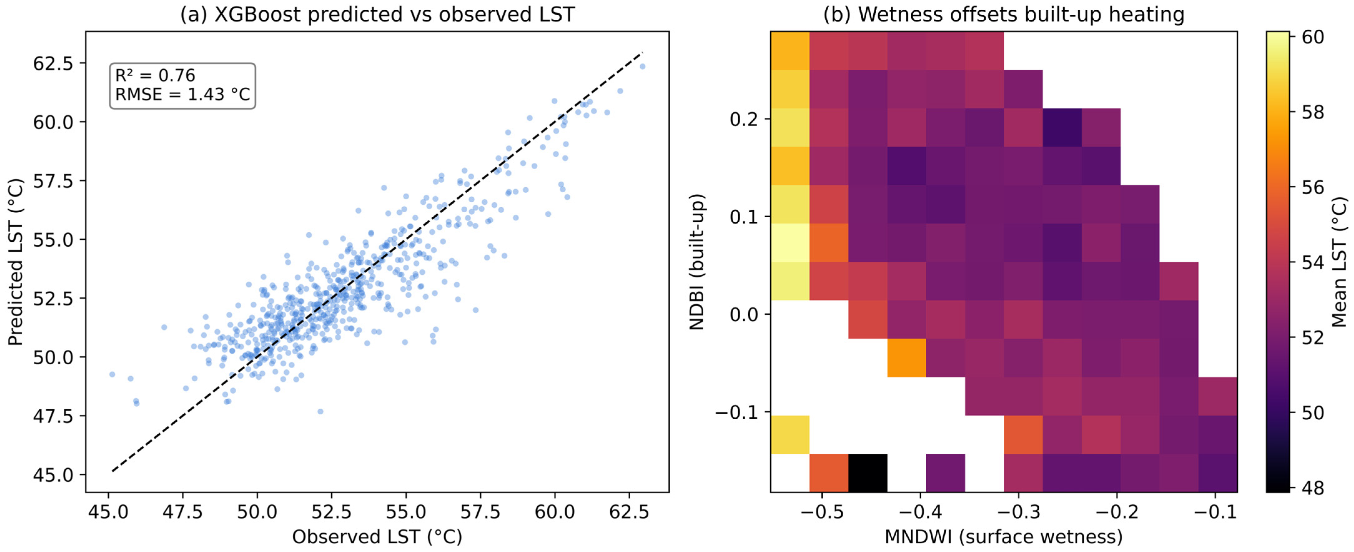
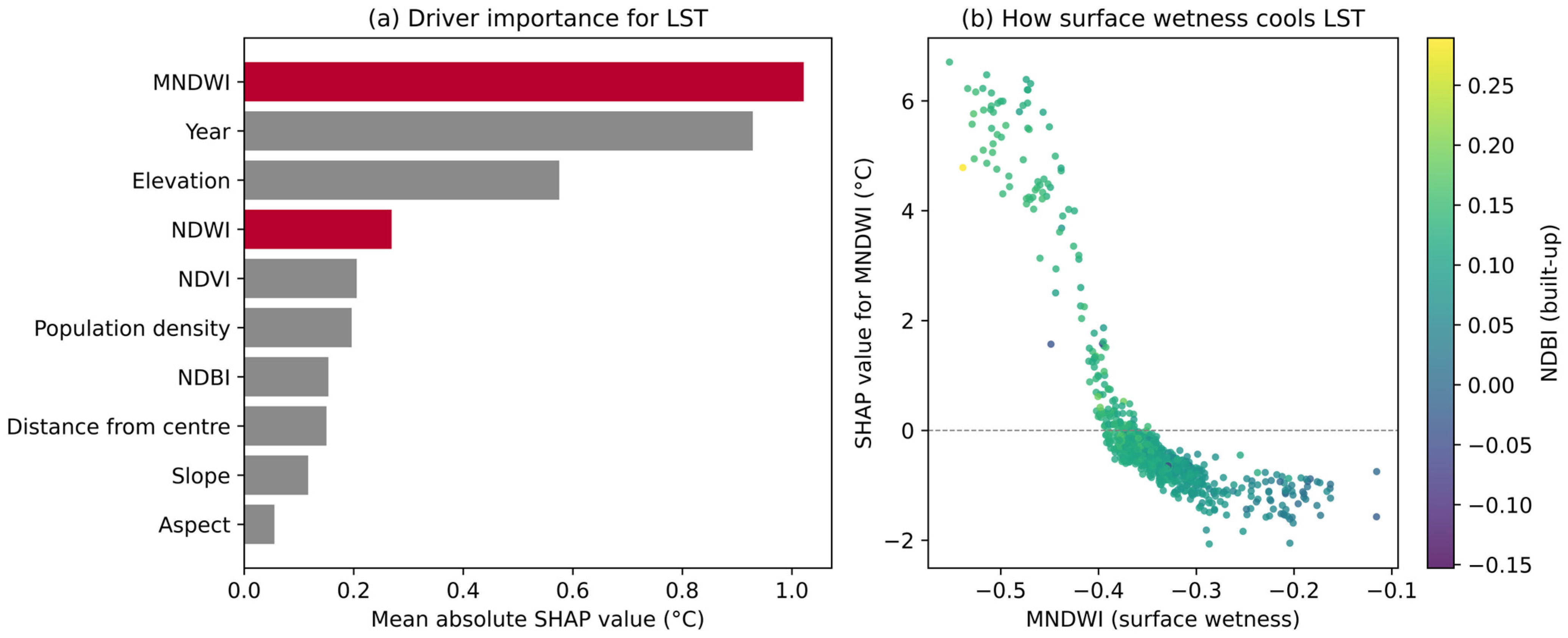
The five algorithms reproduced LST with consistent skill on the held-out test set, with R² ranging from 0.71 to 0.76; XGBoost performed best (R² = 0.76, RMSE = 1.43 °C, MAE = 1.08 °C), and five-fold cross-validation confirmed stability (cross-validated R² ≈ 0.75, standard deviation ≤ 0.03). UHI intensity was predicted with comparable accuracy (R² = 0.68–0.72) (Figure 11a,

Table 8. GeoAI regression performance for LST and UHI intensity: held-out test metrics, random five-fold cross-validation, and spatially blocked (4 × 4 grid) cross-validation.

Target	Model	Test R2	Test RMSE	Random CV R2 (±SD)	Spatial CV R2 (±SD)	Spatial RMSE	Spatial MAE
LST	Random Forest	0.714	1.572	0.717 ± 0.033	0.453 ± 0.103	1.957	1.480
LST	Extra Trees	0.736	1.510	0.723 ± 0.028	0.484 ± 0.106	1.889	1.457
LST	Gradient Boosting	0.723	1.547	0.707 ± 0.026	0.483 ± 0.106	1.897	1.482
LST	Histogram Gradient Boosting	0.739	1.501	0.728 ± 0.031	0.440 ± 0.114	1.971	1.505
LST	XGBoost	0.764	1.426	0.748 ± 0.025	0.499 ± 0.104	1.864	1.439
UHI	Random Forest	0.689	0.029	0.695 ± 0.042	0.337 ± 0.190	0.037	0.028
UHI	Extra Trees	0.712	0.028	0.700 ± 0.032	0.367 ± 0.186	0.036	0.027
UHI	Gradient Boosting	0.684	0.030	0.668 ± 0.030	0.343 ± 0.197	0.036	0.028
UHI	Histogram Gradient Boosting	0.695	0.029	0.696 ± 0.040	0.327 ± 0.202	0.037	0.028
UHI	XGBoost	0.723	0.028	0.709 ± 0.033	0.373 ± 0.192	0.036	0.028

). These values are characteristic of an honest remote-sensing model trained without information leakage; the thermal-stress classification, with the target removed from the predictors, reached a realistic 64–67% cross-validated accuracy. Model attribution placed surface-water wetness at the center of the thermal regime as follows: in the SHAP analysis MNDWI was the single most influential predictor (mean absolute SHAP = 1.03 °C), ahead of the temporal term and elevation, with NDWI also in the upper tier (Figure 12). The two-dimensional response surface shows that increasing wetness lowered LST across all levels of built-up density, confirming that surface water can offset built-up heating (Figure 11b). Under spatially blocked cross-validation, in which entire map blocks were withheld from training, performance declined to R² = 0.44–0.50 for LST (best: XGBoost, 0.50 ± 0.10) and 0.33–0.37 for UHI intensity (Table 8). The contrast between the random and blocked estimates quantifies the influence of spatial autocorrelation as follows: random cross-validation describes interpolation skill within sampled neighborhoods, whereas the blocked estimates provide a conservative bound for transfer to unsampled districts. Predictive claims in this study are therefore restricted to interpolation within the sampled domain; the wetness–temperature relationships in Section 3.7 do not depend on the validation scheme.

Because the four spectral indices share spectral bands, they are strongly collinear (MNDWI variance inflation factor = 1251; condition index = 95), so individual coefficients in a four-index linear model are unstable. Three complementary analyses confirm that the wetness signal is nonetheless robust. The partial correlation between MNDWI and LST, controlling for NDVI and NDBI, remained strong (r = −0.56, p < 0.001), as did that with UHI intensity (r = −0.60). In a reduced multivariable model that omitted the redundant NDWI and in which all VIF were below nine, MNDWI carried the largest standardized effect on LST (beta = −1.35), roughly double that of NDVI or NDBI. Across the five cross-validation folds, MNDWI was ranked the most important predictor in every fold, and the two water indices together accounted for 38 ± 1% of total SHAP importance. The ordinary least-squares slope of LST on MNDWI was −2.2 °C per 0.1 unit (95% CI −2.4 to −2.0 °C), stable in sign across both years (−2.6 °C in 2014; −2.1 °C in 2024) and negative in all sixteen spatial blocks. Predictive skill was insensitive to the population layer (random-CV LST R2 of 0.74 with versus 0.71 without WorldPop) and increased modestly with finer spatial blocks (blocked LST R2 of 0.24, 0.50 and 0.54 for 3 × 3, 4 × 4 and 5 × 5 grids), so the reported 4 × 4 estimate is conservative rather than an artifact of block size.

3.9. Thermal-Environmental Zonation

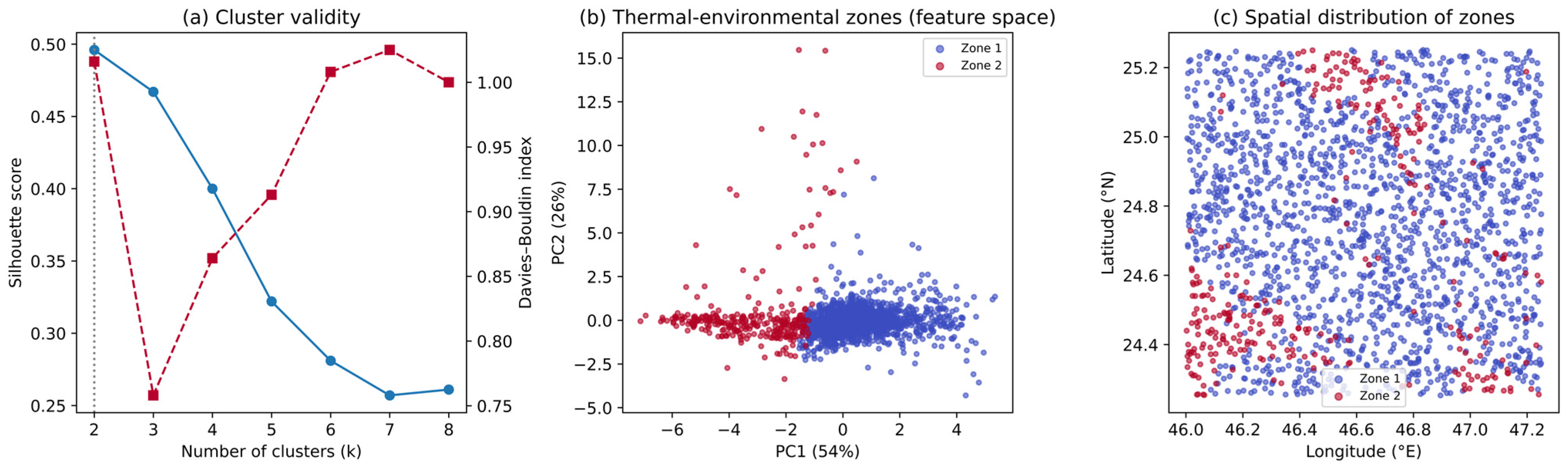
K-means clustering of the 2000 points on their standardized NDVI, NDBI, MNDWI, NDWI, LST, and UHI values produced an optimal two-zone partition. The silhouette coefficient peaked at k = 2 (0.50) and declined steadily for larger k, while the Davies–Bouldin and Calinski–Harabasz indices indicated no superior higher-k solution (Figure 13a). The two zones differ primarily in wetness and temperature (

Table 9. Mean characteristics of the two thermal-environmental zones identified by K-means clustering.

Zone	n	NDVI	NDBI	MNDWI	NDWI	LST (°C)	UHI
1 (cooler, moister)	1695	0.092	0.102	−0.328	−0.234	52.06	−0.014
2 (hotter, drier)	305	0.136	0.111	−0.434	−0.340	57.26	0.083

). Zone 1, comprising the large majority of the metropolis (n = 1695), is comparatively moister (mean MNDWI −0.33) and cooler (mean LST 52.1 °C), whereas Zone 2 (n = 305) is markedly drier (MNDWI −0.43) and hotter (57.3 °C); the hotter zone is not the least vegetated, since its mean NDVI is in fact slightly higher, reinforcing that wetness rather than greenness tracks the thermal field. DBSCAN identified a single dominant density cluster with only 72 noise points, consistent with a wetness-temperature continuum rather than many discrete groups (Figure 13b,c).

3.10. Surface-Water Cooling Gradient Along the Wadi Hanifah Corridor

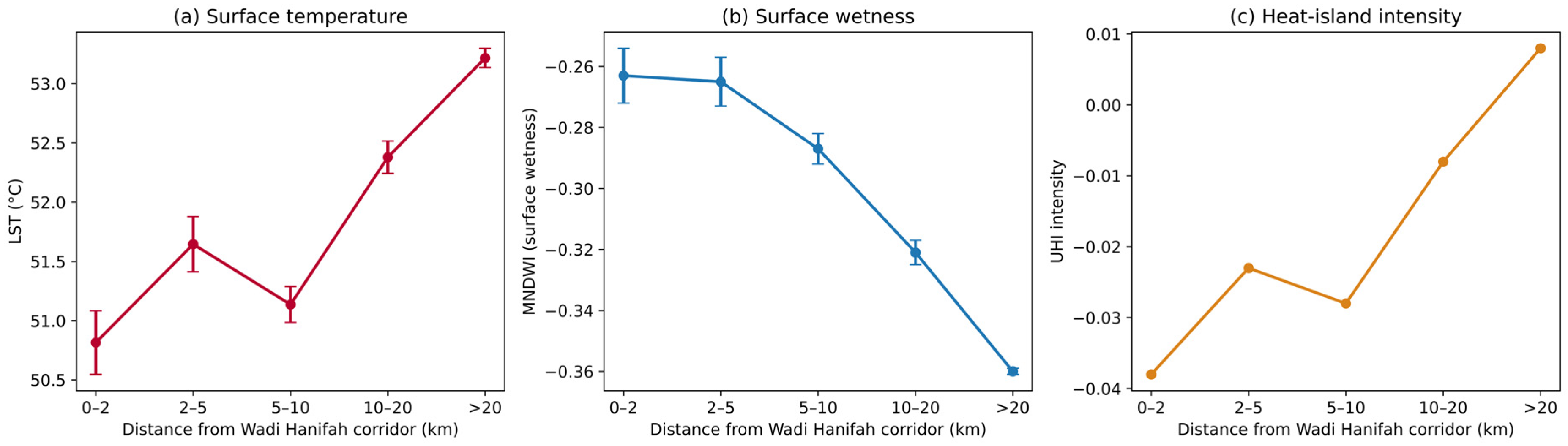
To translate the wetness signal into corridor-scale guidance, we examined how thermal and wetness conditions vary with distance from the Wadi Hanifah corridor. Distance was negatively related to surface wetness (r = −0.41, p < 0.001) and positively related to temperature (LST r = 0.22, p < 0.001), so locations nearer the corridor are both moister and cooler (Figure 14). Mean LST rose from 50.8 °C within 2 km of the corridor to 53.2 °C beyond 20 km, a gradient of roughly 2.4 °C, while mean MNDWI fell from −0.26 to −0.36, and UHI intensity shifted from negative (cooler than the city mean) near the corridor to positive far from it. Although the corridor center-line is approximated and near-corridor sample sizes are modest, the gradient is consistent across all three variables and significant on the full sample, providing distance-explicit evidence that proximity to a rehabilitated wadi-wetland corridor confers measurable cooling.

4. Discussion

Our results position surface-water wetness as the leading remotely sensed control on LST in arid Riyadh, a finding with direct relevance to wetland and blue–green planning in drylands. The negative MNDWI–LST relationship (r = −0.48) and the dominance of MNDWI in the SHAP attribution are consistent with the evaporative-cooling mechanism reported for water bodies and wetlands in humid cities [9,10], and they extend that mechanism to a setting where open water is effectively absent. The absence of any open-water pixels across 2000 samples, combined with a 1.99 °C rise in LST over the decade, indicates that Riyadh’s capacity to buffer heat through surface moisture is severely limited. For planners, the implication is concrete: rehabilitated wadi-wetland corridors such as Wadi Hanifah and engineered blue–green features that raise surface wetness act on the variable our models and identify them as most influential.

4.1. Urban Thermal Dynamics and Vegetation Loss in an Arid Environment

This study highlights a notable rise in urban heat in Riyadh from 2014 to 2024, with very high UHI areas expanding from 13.70% to 32.49%, along with a concerning loss of 302.26 km² of vegetation. These findings are in line with recent trends seen in other fast-growing GCC cities, where urban heat effects have become more intense due to rapid growth [4,48]. The 18.79 percentage-point increase in very high UHI areas in Riyadh is even more substantial than in many temperate cities, highlighting the severe thermal stress faced by arid urban areas under extreme climatic conditions [6].

Vegetation greenness showed only a weak association with surface temperature in this study (NDVI–LST r = 0.08), whereas surface-water wetness was strongly and negatively related to thermal stress (MNDWI–LST r = −0.48; MNDWI–UHI r = −0.53). This pattern is consistent with Almalki et al. [21], who show that water availability constrains vegetation cooling in dry regions, and it contrasts with the stronger NDVI–LST correlations (r below −0.50) typical of temperate cities. The implication is that cooling strategies in arid cities should target surface moisture directly, through water-retaining landscapes and irrigated blue–green corridors, rather than greenness alone [9,10]. The positive LST–NDBI relationship (r = 0.27) confirms built-up heating, but its magnitude is secondary to the wetness gradient.

Over the decade, built-up areas expanded by 323.56 km², which means an urbanization rate of 32.36 km² per year. This growth is similar to what we have seen in other fast-growing cities in Saudi Arabia, where urban expansion often exceeds 25 km² annually [8]. At the same time, the loss of vegetation covering 302.26 km² is a significant environmental concern, as it worsens thermal stress beyond the effects of urban growth alone. Despite some efforts to introduce nearby green spaces, the overall development pattern in Riyadh has not fully incorporated green infrastructure to mitigate heat and other thermal challenges caused by expanding urban areas [7]. The Green Riyadh program is the city’s main response, aiming to raise green cover from roughly 1.5% to 9% and to plant more than 7.5 million trees by 2030 [54]. Its effect on temperature is not yet visible at the city scale. Imam [55] found that vegetated area in Riyadh did not grow between 2018 and 2022 even as the area under urban heat expanded, and Moscatelli and Raffa [56] describe the city’s green infrastructure as still moving from plans to practice. This is consistent with Alajizah and Altuwaijri [48], who linked Riyadh’s rapid expansion to a clear decline in environmental conditions.

4.2. Model Performance, Spatial Generalization and Explainability

The ensemble algorithms predicted LST with test R² of 0.71–0.76 and UHI intensity with 0.68–0.72 under random cross-validation, with XGBoost performing best (RMSE = 1.43 °C). Under spatially blocked validation, performance declined to R² = 0.44–0.50 for LST and 0.33–0.37 for UHI, which bounds the framework’s transferability to unsampled districts and makes the role of spatial autocorrelation explicit rather than assumed [40]. These values are deliberately free of target leakage: neither LST nor UHI, nor any category derived from them, was supplied as a predictor, and the thermal-stress classification reached a realistic 64–67% cross-validated accuracy with the target variables excluded. The two validation schemes address different questions, and both are reported so that readers can assess interpolation and extrapolation skills separately. Importantly, the precedence of surface-water wetness over vegetation does not rest on bivariate correlation alone: it is reproduced by partial correlations controlling for NDVI and NDBI, by a reduced multivariable model with acceptable collinearity, and by SHAP rankings that are stable across all cross-validation folds.

The SHAP attribution [27] identified surface-water wetness (MNDWI) as the most influential predictor of LST, with a mean absolute contribution of 1.03 °C, ahead of the temporal term and elevation, and with NDWI also in the upper tier. The convergence of the correlation, regression and attribution analyses on the same variable strengthens the plausibility of an evaporative-cooling mechanism, although attribution values describe model behavior rather than confirmed physical causation. No prediction-interval or calibration analysis was undertaken; uncertainty is conveyed through cross-validated dispersion, and probabilistic prediction remains a development priority before the framework is used for risk-averse infrastructure decisions.

This study advances urban thermal research in Gulf cities by pairing explainable ML with an explicitly spatial validation design, and by quantifying, for the first time in an arid Gulf metropolis, the dominance of surface-water wetness over greenness and built-up density as a control on LST.

4.3. Surface Wetness Gradients and Blue–Green Planning Applications

The wetness–temperature response surface (Figure 11b) shows that higher MNDWI is associated with lower LST across all levels of built-up density, indicating that moisture-led interventions retain their cooling value even in densely developed districts. The binned wetness gradient (Figure 10a) translates this into planning terms as follows: each 0.1 increase in MNDWI corresponds to approximately 2.2 °C lower surface temperature. Because open water was absent from all 2000 samples, the observed cooling operates entirely through soil and vegetation moisture; restoring even modest surface-water presence along the Wadi Hanifah corridor would extend the upper end of a wetness gradient that the city currently lacks [9].

These gradients provide a screening tool for prioritizing blue–green investment [17]. Districts that combine high NDBI with strongly negative MNDWI occupy the hottest corner of the response surface and represent the highest-value targets for moisture-led cooling, whereas districts that are already comparatively moist yield smaller marginal gains. Reading interventions off a continuous, physically interpretable surface avoids the arbitrariness of discrete zonation schemes. Concrete blue-green measures suited to this setting include vegetated wadi buffers and check-dams that retain seasonal flow, treated-wastewater-irrigated street trees and pocket parks, bioswales and permeable surfaces that raise near-surface soil moisture, and shaded water features along the Wadi Hanifah corridor.

4.4. Practical Implications for Cooling and Urban Planning

These findings carry clear implications for climate-resilient planning in Riyadh and similar arid cities. The expansion of very high UHI intensity areas from 13.70% to 32.49% of the study area indicates that thermal stress is outpacing mitigation, and the wetness gradient offers a quantitative basis for response as follows: interventions that raise MNDWI by 0.1 in the hottest districts are associated with roughly 2 °C lower surface temperature [57]. Corresponding reductions in cooling demand are expected, but building-level energy savings were not modeled here and remain to be quantified.

Translating these gradients into practice implies differentiated requirements as follows: moisture-retaining landscaping and high-albedo surfaces in the hottest, driest districts [57]; protection of existing wet and vegetated corridors from conversion; and routine monitoring of MNDWI and NDWI as planning indicators, which Landsat provides freely at 30 m resolution.

4.5. Policy Recommendations for Climate-Resilient Urban Development

The central policy implication is to treat surface moisture as cooling infrastructure. Specific measures include protecting and rehydrating the Wadi Hanifah and Wadi Al-Ha’ir corridors, requiring water-efficient irrigated greenery in new developments, reusing treated wastewater to sustain urban wetness, and incorporating water-index monitoring into municipal heat-action plans [4,57]. Quantified energy-saving targets should be set only after thermal predictions are coupled with building energy models; this study deliberately refrains from asserting unverified percentages. Because potable water is scarce, these interventions should draw on non-potable sources, treated wastewater reuse, stormwater harvesting in the wadi network, and managed aquifer recharge, which are increasingly deployed in Gulf cities. The humidity-heat trade-off must also be weighed: while added moisture lowers surface temperature, it can raise humidity-based heat-stress indices, so designs should favor shaded, ventilated blue-green configurations rather than open standing water alone.

The workflow is transferable: it relies entirely on free, global data (Landsat Collection 2, SRTM, WorldPop) processed in Google Earth Engine, and the spatially blocked validation provides an honest template for assessing how far models trained in one part of a city extend to another. Application to other arid metropolises requires recalibration of class boundaries and renewed validation rather than direct transfer of coefficients.

4.6. Limitations

This study offers valuable insights into surface-water wetness and urban thermal stress in arid environments; however, several limitations related to temporal scope and implementation must be acknowledged. A primary temporal limitation is the dependence on satellite imagery from July, which captures peak summer conditions but does not represent the thermal behavior throughout the entire year or seasonal variations in UHI intensity. While July is a critical design consideration for cooling infrastructure and energy demand in Riyadh’s extreme climate [7], comparable studies in similar arid regions have documented seasonal UHI fluctuations of 3–5 °C, with distinct spatial patterns observed during cooler months—particularly when nocturnal heat retention becomes more significant [44,45]. Consequently, a more comprehensive seasonal analysis would improve understanding of the temporal dynamics of UHI and the relative efficacy of mitigation strategies throughout different times of the year. The study’s temporal resolution—two time points separated by a decade—captures long-term urban transformation but limits the ability to assess year-to-year variability, extreme weather events, or transitional development phases. Annual or biennial analysis would enable more detailed attribution of thermal changes to specific urban projects or policy interventions, supporting adaptive management and accountability [41,48]. Future research should use multi-seasonal satellite imagery to study winter UHI, night-time thermal patterns, and seasonal changes. This aids in creating seasonally adaptive energy strategies and finding year-round thermal refuges. Including meteorological data—like wind, humidity, and solar radiation—would enhance energy models by considering atmospheric conditions beyond surface temperature [11,37]. Beyond temporal scope, four further limitations warrant emphasis. First, spatially blocked cross-validation shows that predictive skill declines when models extrapolate to unsampled blocks (LST R² ≈ 0.50), so predictions outside sampled neighborhoods carry wider uncertainty. Second, the area-change statistics derive from single-composite classifications whose class boundaries condition the reported percentages; values quoted to fractions of a square kilometer are indicative. Third, the 2024 population layer is approximated by the 2020 WorldPop release. Fourth, no in situ temperature or flux observations were available for ground validation.

From an implementation perspective, several challenges may hinder applying these findings in policy and practice. Landsat imagery’s spatial resolution (30 m, 100 m thermal resampled) might be too coarse for building-level applications, especially in heterogeneous urban areas. Higher-resolution thermal data from airborne or future satellite platforms could improve accuracy but involve higher costs and logistical challenges [11,37]. Policy implementation needs coordinated governance, with agencies collaborating to translate thermal zones into building codes and zoning. Fragmented structures and unclear roles hinder adoption despite strong evidence [58]. Enforcement barriers include limited inspection, lack of expertise, and developer resistance over costs. Solutions involve capacity building, standard protocols, and incentives [32,57]. Achieving thermal cooling in arid cities requires water infrastructure investments like irrigation, greywater recycling, and desalination, adding costs [21,45]. Economic analysis is essential for cost-effectiveness and fair benefits. While energy savings are measurable, upfront costs for buildings, district cooling, and green spaces may need subsidies. A comprehensive cost–benefit analysis of energy, environmental, and public health outcomes can guide decisions [20,33].

4.7. Future Research Directions

Several research directions would extend this work. First, coupling the thermal predictions with building energy simulation would convert wetness-led cooling into quantified energy and cost outcomes, enabling the cost–benefit analysis this study intentionally does not claim [28,58]. Second, denser time series, including Sentinel-2 and SAR-based wetness retrievals that are insensitive to cloud, would resolve the full seasonal hydroperiod and test whether the wetness–temperature relationship holds outside peak summer. Third, models with explicit spatial structure, such as graph-based or convolutional architectures that represent neighborhood context, would address the absence of spatial inductive bias in tabular ensembles and could narrow the gap between random and spatially blocked performance. Fourth, in situ microclimate monitoring along the Wadi Hanifah corridor would provide the ground truth needed to convert the observed associations into validated process understanding. Finally, our thermal target is land surface temperature; translating wetness-driven cooling into human heat exposure will require thermal-comfort indices such as the Universal Thermal Climate Index (UTCI) or wet-bulb temperature [59], which depend on air temperature, humidity and wind that cannot be retrieved from Landsat alone, making field-coupled monitoring a priority for follow-up.

5. Conclusions

This research repositions surface-water wetness as the central, measurable lever of urban heat mitigation in an arid metropolis. Using 2000 real Landsat sample points for 2014 and 2024, five ensemble algorithms predicted LST with R² of 0.71–0.76 under random cross-validation and 0.44–0.50 under spatially blocked validation, and SHAP attribution identified MNDWI as the dominant thermal driver, ahead of elevation, vegetation and built-up density. Each 0.1 increase in surface wetness was associated with approximately 2.2 °C lower surface temperature, while point-level LST rose by 1.99 °C over the decade, and very-high UHI intensity areas expanded from 13.70% to 32.49% of the study area. The absence of open water across all samples quantifies the hydrological deficit underlying Riyadh’s intensifying heat.

For planners and policymakers, the recommendations are concrete: protect and rehydrate wadi-wetland corridors, prioritize moisture-led interventions in districts that combine high built-up density with low wetness, and adopt MNDWI and NDWI as routine monitoring indicators of cooling capacity. The workflow extends to other arid cities via free global data and cloud-based processing, with spatially constrained validation providing an honest measure of where predictions can be trusted. The principal limitations, peak-summer scope, an approximated 2024 population layer, and reduced extrapolation skill across unsampled blocks, define the agenda for future work, particularly SAR-based hydroperiod monitoring and in situ validation. As arid cities grow hotter, water, not greenness alone, is the resource on which their thermal resilience depends.

References

1. Aboulnaga, M.; Trombadore, A.; Mostafa, M.; Abouaiana, A. Assessment of Urban Heat Island in Conjunction with Green Coverage in Large Cities: Cairo, Egypt, and Rome, Italy. In Livable Cities; Springer International Publishing: Berlin/Heidelberg, Germany, 2024; pp. 495–617. [Google Scholar] [CrossRef]
2. Haq, S.M.A. Urban Green Spaces and an Integrative Approach to Sustainable Environment. J. Environ. Prot. 2011, 2, 601–608. [Google Scholar] [CrossRef]
3. El-Hamid, H.T.A.; Arshad, M.; Eid, E.M. The effects of coastal development on the urban heat island in the mangrove ecosystem along the Jazan coast, KSA. J. Coast. Conserv. 2022, 26, 70. [Google Scholar] [CrossRef]
4. Abulibdeh, A. Analysis of urban heat island characteristics and mitigation strategies for eight arid and semi-arid gulf region cities. Environ. Earth Sci. 2021, 80, 259. [Google Scholar] [CrossRef] [PubMed]
5. Huang, K.; Li, X.; Liu, X.; Seto, K.C. Projecting global urban land expansion and heat island intensification through 2050. Environ. Res. Lett. 2019, 14, 114037. [Google Scholar] [CrossRef]
6. Alghamdi, A.S. An integrated ML-powered geospatial analysis of surface urban heat island and its mitigation in Riyadh City, Saudi Arabia. Urban Clim. 2025, 64, 102642. [Google Scholar] [CrossRef]
7. Aina, Y.A.; Parvez, I.M.; Balogun, A.L.; Adam, E. Urban Heat Island Effects and Mitigation Strategies in Saudi Arabian Cities. In Advances in 21st Century Human Settlements; Springer: Berlin/Heidelberg, Germany, 2021; pp. 235–248. [Google Scholar] [CrossRef] [PubMed]
8. Alshayeb, M.J.; Bindajam, A.A.; Mallick, J.; Shohan, A.A.A. Integrating fuzzy logic and land use dynamics to delineate urban heat island formation zones and assess land surface temperature changes over three decades: A case study of Asir region, Saudi Arabia. Stoch. Environ. Res. Risk Assess. 2025, 39, 3761–3780. [Google Scholar] [CrossRef]
9. Xu, H. Modification of normalised difference water index (NDWI) to enhance open water features in remotely sensed imagery. Int. J. Remote Sens. 2006, 27, 3025–3033. [Google Scholar] [CrossRef]
10. McFeeters, S.K. The use of the Normalized Difference Water Index (NDWI) in the delineation of open water features. Int. J. Remote Sens. 1996, 17, 1425–1432. [Google Scholar] [CrossRef]
11. de Almeida, C.R.; Teodoro, A.C.; Gonçalves, A. Study of the urban heat island (Uhi) using remote sensing data/techniques: A systematic review. Environments 2021, 8, 105. [Google Scholar] [CrossRef]
12. Lyu, F.; Wang, S.; Han, S.Y.; Catlett, C.; Wang, S. An integrated cyberGIS and machine learning framework for fine-scale prediction of Urban Heat Island using satellite remote sensing and urban sensor network data. Urban Inform. 2022, 1, 6. [Google Scholar] [CrossRef] [PubMed]
13. Bakirci, M. Smart city air quality management through leveraging drones for precision monitoring. Sustain. Cities Soc. 2024, 106, 105390. [Google Scholar] [CrossRef]
14. Mai, G.; Xie, Y.; Jia, X.; Lao, N.; Rao, J.; Zhu, Q.; Liu, Z.; Chiang, Y.Y.; Jiao, J. Towards the next generation of Geospatial Artificial Intelligence. Int. J. Appl. Earth Obs. Geoinf. 2025, 136, 104368. [Google Scholar] [CrossRef]
15. Lodhi, M.K.; Tan, Y.; Suprijanto, A.; Naeem, S.; Li, Y. GeoAI-Driven mapping of urban rooftop Photovoltaics: A sustainable energy framework for Karachi, Pakistan. Int. J. Appl. Earth Obs. Geoinf. 2025, 143, 104786. [Google Scholar] [CrossRef]
16. Chen, Y.; Shan, B.; Yu, X. Study on the spatial heterogeneity of urban heat islands and influencing factors. Build. Environ. 2022, 208, 108604. [Google Scholar] [CrossRef]
17. Budzik, G.; Sylla, M.; Kowalczyk, T. Understanding Urban Cooling of Blue-Green Infrastructure: A Review of Geospatial Data and Planning Optimization Methods for Mitigating Urban Heat Islands. Sustainability 2024, 17, 142. [Google Scholar] [CrossRef]
18. Islam, M.T.; Ali, A. Sustainable green energy transition in Saudi Arabia: Characterizing policy framework, interrelations and future research directions. Next Energy 2024, 5, 100161. [Google Scholar] [CrossRef]
19. Zhang, M. A global perspective on urban thermal environment: From satellite data to sustainable development. Cell Rep. Sustain. 2025, 2, 100522. [Google Scholar] [CrossRef]
20. Rehman, H.S.U.; Alamgir, S.; Khan, M.A.; Masood, R.; Sammad, M.H.; Roy, K. Urban Heat Island Mitigation by LEED and BIM Integration—A Review. Buildings 2025, 15, 2523. [Google Scholar] [CrossRef]
21. Almalki, R.; Khaki, M.; Saco, P.M.; Rodriguez, J.F. Monitoring and Mapping Vegetation Cover Changes in Arid and Semi-Arid Areas Using Remote Sensing Technology: A Review. Remote Sens. 2022, 14, 5143. [Google Scholar] [CrossRef]
22. Ahmed, A.N.; AlDahoul, N.; Aziz, N.A.; Huang, Y.F.; Sherif, M.; El-Shafie, A. The urban heat Island effect: A review on predictive approaches using artificial intelligence models. City Environ. Interact. 2025, 28, 100234. [Google Scholar] [CrossRef]
23. Tanoori, G.; Soltani, A.; Modiri, A. Machine Learning for Urban Heat Island (UHI) Analysis: Predicting Land Surface Temperature (LST) in Urban Environments. Urban Clim. 2024, 55, 101962. [Google Scholar] [CrossRef]
24. Mallick, J.; Alqadhi, S. Explainable artificial intelligence models for proposing mitigation strategies to combat urbanization impact on land surface temperature dynamics in Saudi Arabia. Urban Clim. 2025, 59, 102259. [Google Scholar] [CrossRef]
25. Rasul, A. Artificial intelligence-enabled assessment of urban growth impacts on land surface temperature in a hot desert climate: A case study of Baghdad city. Asian Geogr. 2025, 42, 159–180. [Google Scholar] [CrossRef]
26. Tehrani, A.A.; Veisi, O.; Kia, K.; Delavar, Y.; Bahrami, S.; Sobhaninia, S.; Mehan, A. Predicting urban Heat Island in European cities: A comparative study of GRU, DNN, and ANN models using urban morphological variables. Urban Clim. 2024, 56, 102061. [Google Scholar] [CrossRef]
27. Lundberg, S.M.; Lee, S.-I. A unified approach to interpreting model predictions. Adv. Neural Inf. Process. Syst. 2017, 30, 4765–4774. [Google Scholar]
28. Bansal, P.; Quan, S.J. Examining temporally varying nonlinear effects of urban form on urban heat island using explainable machine learning: A case of Seoul. Build. Environ. 2024, 247, 110957. [Google Scholar] [CrossRef]
29. Sheng, T.; Zhang, Z.; Qian, Z.; Ma, P.; Xie, W.; Zeng, Y.; Zhang, K.; Sun, Z.; Yu, J.; Chen, M. Examining urban agglomeration heat island with explainable AI: An enhanced consideration of anthropogenic heat emissions. Urban Clim. 2025, 59, 102251. [Google Scholar] [CrossRef]
30. Oukawa, G.Y.; Krecl, P.; Targino, A.C.; Batista, L.F.A. Advantages of modeling the urban heat island intensity: A tool for implementing nature-based solutions. Sustain. Cities Soc. 2024, 102, 105204. [Google Scholar] [CrossRef]
31. Rana, B.; Bandyopadhyay, J.; Halder, B. Investigating the relationship between urban sprawl and urban heat island using remote sensing and machine learning approaches. Theor. Appl. Climatol. 2024, 155, 4161–4188. [Google Scholar] [CrossRef]
32. Rashtian, Z.; Manesh, M.T.; Tahsildoost, M.; Zomorodian, Z.S. Data-driven real-time visualization of urban heat islands using mean radiant temperature for urban design. Energy Build. 2025, 333, 115470. [Google Scholar] [CrossRef]
33. Moya, D.; Copara, D.; Giarola, S.; Hawkes, A. Global datasets of geospatial-AI-resolved energy consumers including climate-driven energy demands, geographical and socioeconomic realities for a transition reset. Sci. Data 2024, 11, 1408. [Google Scholar] [CrossRef] [PubMed]
34. Ernst, E.; Srivastava, A.; Bilel, Z.; Abdo, H.; Forouheshfar, Y.; Ayadi, R.; Moghadas, O. Enhancing system resilience to climate change through artificial intelligence: A systematic literature review. Front. Clim. 2025, 7, 1585331. [Google Scholar] [CrossRef]
35. Shatnawi, N.; Alqaralleh, R.M.; Tarawneh, E.R. Urban heat island in Amman: AI-based modeling of urban morphology and green infrastructure in mitigating thermal stress. Environ. Earth Sci. 2025, 84, 498. [Google Scholar] [CrossRef]
36. Kılınç, M.; Aydın, C.; Aydın, G.E.; Balcı, D. HeatWatch: Identification of Parameters Influencing the Urban Heat Island Effect through Deep Learning Techniques. Int. Arch. Photogramm. Remote Sens. Spat. Inf. Sci. 2024, 48, 107–112. [Google Scholar] [CrossRef]
37. Bushenkova, A.; Soares, P.M.M.; Johannsen, F.; Lima, D.C.A. Towards an improved representation of the urban heat island effect: A multi-scale application of XGBoost for madrid. Urban Clim. 2024, 55, 101982. [Google Scholar] [CrossRef]
38. Amrulloh, I.; Fikriyah, V.N. Time series analysis of landsat data for urban heat island monitoring in Semarang City. IOP Conf. Ser. Earth Environ. Sci. 2024, 1314, 012086. [Google Scholar] [CrossRef]
39. Duan, X.; Haseeb, M.; Tahir, Z.; Mahmood, S.A.; Tariq, A.; Jamil, A.; Ullah, S.; Abdullah-Al-Wadud, M. A geospatial and statistical analysis of land surface temperature in response to land use land cover changes and urban heat island dynamics. Sci. Rep. 2025, 15, 4943. [Google Scholar] [CrossRef] [PubMed]
40. Roberts, D.R.; Bahn, V.; Ciuti, S.; Boyce, M.S.; Elith, J.; Guillera-Arroita, G.; Hauenstein, S.; Lahoz-Monfort, J.J.; Schröder, B.; Thuiller, W.; et al. Cross-validation strategies for data with temporal, spatial, hierarchical, or phylogenetic structure. Ecography 2017, 40, 913–929. [Google Scholar] [CrossRef]
41. Khalil, M.; Kumar, J.S. Time-series studies of land surface temperature in Damascus, Syria through MODIS by Google Earth Engine. Adv. Space Res. 2025, 75, 1960–1973. [Google Scholar] [CrossRef]
42. Elabd, E.; Hamouda, H.M.; Ali, M.A.M.; Fouad, Y. Climate change prediction in Saudi Arabia using a CNN GRU LSTM hybrid deep learning model in al Qassim region. Sci. Rep. 2025, 15, 16275. [Google Scholar] [CrossRef] [PubMed]
43. Dahy, B.; Al-Memari, M.; Al-Gergawi, A.; Burt, J.A. Remote sensing of 50 years of coastal urbanization and environmental change in the Arabian Gulf: A systematic review. Front. Remote Sens. 2024, 5, 1422910. [Google Scholar] [CrossRef]
44. Alghamdi, A.S.; Moore, T.W. Detecting Temporal Changes in Riyadh’s Urban Heat Island. Pap. Appl. Geogr. 2015, 1, 312–325. [Google Scholar] [CrossRef]
45. Al-Saadi, L.M.; Jaber, S.H.; Al-Jiboori, M.H. Variation of urban vegetation cover and its impact on minimum and maximum heat islands. Urban Clim. 2020, 34, 100707. [Google Scholar] [CrossRef]
46. Ghasemi, K.; Al-Zubaidi, A.M.J.; Qelichi, M.M.; Dolatkhahi, K. Understanding urban sprawl in Baqubah, Iraq: A study of influential factors. J. Urban Manag. 2025, 14, 787–812. [Google Scholar] [CrossRef]
47. Aina, Y.A.; Adam, E.M.; Ahmed, F. Spatiotemporal variations in the impacts of urban land use types on urban heat island effects: The case of Riyadh, Saudi Arabia. Int. Arch. Photogramm. Remote Sens. Spat. Inf. Sci. 2017, 42, 9–14. [Google Scholar] [CrossRef]
48. Alajizah, S.M.; Altuwaijri, H.A. Assessing the Impact of Urban Expansion on the Urban Environment in Riyadh City (2000–2022) Using Geospatial Techniques. Sustainability 2024, 11, 4799. [Google Scholar] [CrossRef]
49. Jumari, N.A.S.K.; Ahmed, A.N.; Huang, Y.F.; Ng, J.L.; Koo, C.H.; Chong, K.L.; Sherif, M.; Elshafie, A. Analysis of urban heat islands with landsat satellite images and GIS in Kuala Lumpur Metropolitan City. Heliyon 2023, 9, e18424. [Google Scholar] [CrossRef] [PubMed]
50. Singh, P.; Verma, P.; Chaudhuri, A.S.; Singh, V.K.; Rai, P.K. Evaluating the relationship between Urban Heat Island and temporal change in land use, NDVI and NDBI: A case study of Bhopal city, India. Int. J. Environ. Sci. Technol. 2024, 21, 3061–3072. [Google Scholar] [CrossRef]
51. Cetin, M.; Kavlak, M.O.; Kurkcuoglu, M.A.S.; Ozturk, G.B.; Cabuk, S.N.; Cabuk, A. Determination of land surface temperature and urban heat island effects with remote sensing capabilities: The case of Kayseri, Türkiye. Nat. Hazards 2024, 120, 5509–5536. [Google Scholar] [CrossRef]
52. Aghazadeh, F.; Mashayekh, H.; Akbari, M.A.; Boroukanlou, S.; Habibzadeh, N.; Ghasemi, M.; Goswami, A. A GIRS-based analysis of urban green space losses with land-use changes and its relationship with surface urban heat island in the city of Tabriz. Adv. Space Res. 2025, 75, 1804–1824. [Google Scholar] [CrossRef]
53. Zargari, M.; Mofidi, A.; Entezari, A.; Baaghideh, M. Climatic comparison of surface urban heat island using satellite remote sensing in Tehran and suburbs. Sci. Rep. 2024, 14, 643. [Google Scholar] [CrossRef] [PubMed]
54. Royal Commission for Riyadh City, Green Riyadh Program. Riyadh, Saudi Arabia, 2024. Available online: https://www.rcrc.gov.sa/en/projects/green-riyadh-project/ (accessed on 1 October 2025).
55. Imam, A. Examining the impact of Green Riyadh Project on alleviating urban heat island effects. J. Umm AL-Qura Univ. Eng. Archit. 2023, 14, 201–211. [Google Scholar] [CrossRef]
56. Moscatelli, M.; Raffa, A. Green infrastructure in arid urban contexts: Transitioning ecologies beyond Green Riyadh. AGATHÓN Int. J. Archit. Art Des. 2023, 13, 75–86. [Google Scholar] [CrossRef]
57. Gao, K.; Haddad, S.; Paolini, R.; Feng, J.; Altheeb, M.; Al Mogirah, A.; Moammar, A.B.; Santamouris, M. The use of green infrastructure and irrigation in the mitigation of urban heat in a desert city. Build. Simul. 2024, 17, 679–694. [Google Scholar] [CrossRef]
58. Feng, W.; Yang, L.E.; Zeng, F.; Jia, J.; Zhang, H.; Wu, Z. Enabling urban climate resilience through integrated optimization of urban design. Front. Sustain. Cities 2025, 7, 1657008. [Google Scholar] [CrossRef]
59. Bröde, P.; Fiala, D.; Blažejczyk, K.; Holmér, I.; Jendritzky, G.; Kampmann, B.; Tinz, B.; Havenith, G. Deriving the operational procedure for the Universal Thermal Climate Index (UTCI). Int. J. Biometeorol. 2012, 56, 481–494. [Google Scholar] [PubMed]
Figure 1. Methodological framework linking Landsat-derived surface-water wetness to urban thermal stress through statistical analysis and explainable ML.
Water 18 01628 g001
Figure 2. Geographic location and urban extent of Riyadh, Saudi Arabia.
Water 18 01628 g002
Figure 3. Spatial distribution of vegetation cover derived from NDVI.
Water 18 01628 g003
Figure 4. Urban development patterns based on NDBI analysis.
Water 18 01628 g004
Figure 5. Change detection maps showing NDVI and NDBI differences between 2014 and 2024.
Water 18 01628 g005
Figure 6. LST distribution across Riyadh demonstrates temporal changes in thermal patterns and intensity of urban heat.
Water 18 01628 g006
Figure 7. UHI intensity maps for 2014 and 2024, showing spatial distribution and temporal evolution of thermal stress zones.
Water 18 01628 g007
Figure 8. Difference maps showing changes between 2014 and 2024 in LST and UHI intensity, highlighting areas of significant thermal modification.
Water 18 01628 g008
Figure 9. Pearson correlations among vegetation, built-up, surface-water and thermal indices across 2000 Landsat sample points (2014 and 2024).
Water 18 01628 g009
Figure 10. LST and UHI intensity against surface-water wetness, for 2014 and 2024: (a) MNDWI versus LST; (b) NDWI versus LST; (c) MNDWI versus UHI intensity; (d) NDWI versus UHI intensity. Red lines are least-squares fits; the black markers in panels (a,b) are binned means with standard errors.
Water 18 01628 g010
Figure 11. (a) XGBoost predicted versus observed LST on the held-out test set. (b) Mean LST as a function of surface-water wetness (MNDWI) and built-up density (NDBI).
Water 18 01628 g011
Figure 12. (a) Mean absolute SHAP contribution of each predictor to LST (surface-water indices highlighted). (b) SHAP dependence of MNDWI colored by built-up density, showing the cooling response.
Water 18 01628 g012
Figure 13. Thermal-environmental zonation. (a) Internal validity (silhouette, Davies–Bouldin) across candidate cluster numbers; (b) the two zones in principal-component space; (c) their spatial distribution.
Water 18 01628 g013
Figure 14. Thermal and wetness gradients with distance from the Wadi Hanifah corridor: (a) land surface temperature, (b) surface wetness (MNDWI), and (c) UHI intensity, by distance band (mean ± standard error).
Water 18 01628 g014