Article

Advancing Detailed Flood Hazard Identification in Alberta, Canada: Insights from Two Recent Flood Studies

1
Barr Engineering Company, 1000 7 Ave. SW #450, Calgary, AB T2P 5L5, Canada
2
Alberta Environment and Protected Areas, Oxbridge Place, 9820-106 St. NW, Edmonton, AB T5K 2J6, Canada
*
Author to whom correspondence should be addressed.
Water 2026, 18(13), 1592; https://doi.org/10.3390/w18131592
Submission received: 18 May 2026 / Revised: 25 June 2026 / Accepted: 27 June 2026 / Published: 30 June 2026

Abstract

The increasing frequency of floods and the severity of their consequences for public safety, infrastructure, and the economy demand improved methods for flood hazard identification. Flood studies that include flood hazard mapping are critical tools for informing emergency response and flood recovery, as well as for land use and mitigation planning. The methodology for such flood studies has evolved, and access to more powerful computational resources and high-resolution base data has contributed to the increased use of two-dimensional hydraulic modelling, where one-dimensional modelling previously was the default. However, local-scale flood studies face real-world constraints, including sparse data, challenging hydrologic conditions, and budget limitations, which can hinder the application of advanced techniques. This study addresses these challenges through innovative, practice-driven solutions in two case studies in Alberta, Canada: a small, partly channelized prairie stream network (Wolf Creek, Lacombe) and a laterally dynamic river on a distributary delta (Swan River, Kinuso). Three core components of flood hazard studies are described: field survey data collection, regional hydrology assessment, and hydraulic modelling. Key findings include demonstrating that LiDAR-derived terrain models alone cannot capture channel conveyance, the importance of low-flow calibration in the absence of high-water marks, the selection of a modelling methodology based on bathymetric and topographic features within a study area, and the development of inflow hydrographs for unsteady-state simulation in flat floodplains.

1. Introduction

Flooding continues to be a significant issue that engages the public, businesses, and governments worldwide. Looking ahead, the flood risk is expected to increase substantially because of rapid urbanization in river floodplains, driven by population growth and migration [1]. Additionally, the projected effects of climate change indicate higher risks of flooding across many regions in the near future [2,3].
Canada is warming at twice the global average rate, with northern regions experiencing three times the global average warming rate [4]. Due to its vast size and diverse geography, these temperature increases are unevenly distributed. Overall, higher temperatures increase the likelihood and intensity of extreme precipitation events, which may lead to severe floods [2]. In Canada, floods are the most frequent natural hazard and rank among the costliest [5]. Riverine floods (i.e., fluvial floods) typically happen when extensive runoff following rainfall causes streams to overflow. However, rapid snowmelt with rain on snow in early spring, as well as freeze-up or break-up ice-jam flooding, could also cause fluvial floods. Urbanization exacerbates the flood risk by reducing vegetation and soil cover, which limits water storage and increases runoff, leading to higher flood peaks and volumes [6].
Flooding presents a clear public safety risk, can damage private property and public infrastructure, and has the potential to disrupt economic activity. Floods can also disrupt transportation networks, hindering evacuation plans as well as access to medical care and other essential services. Assessing network degradation through the lens of emergency response has become an important research area, as road connectivity is critical for emergency vehicles to reach populated areas and those at risk [7,8,9,10,11,12].
An example of widespread flooding in the Canadian context is the June 2013 flooding in Southern Alberta [3]. An intense rainfall event triggered flooding centered west of Calgary, which brought between 200 and 300 mm of accumulated precipitation over two days to some areas. Combined with rapid mountain snowmelt and saturated soils, the event caused catastrophic flooding in multiple communities in the Bow, Elbow and Highwood River basins. In addition to the tragic loss of life, property damage and other financial losses were estimated to amount to CAD 5–6 billion [1,3] of which a sizable portion was due to damage in Calgary, the largest city in Alberta [13].
The 2013 flooding in Southern Alberta renewed public and government interest in flood mapping across Canada, highlighting how flood mapping could be used to inform emergency response and flood recovery efforts, as well as long term land use and mitigation planning [14,15]. It highlighted the benefits of updating older flood maps and expanding coverage to more flood-prone areas and led to increased provincial, territorial, and federal funding for flood mapping initiatives.

1.1. Flood Mapping in Canada

Apart from federal jurisdiction lands, provinces and territories have led the production of flood mapping in Canada, with some assigning responsibilities for flood mapping to regional or municipal entities [16]. Provincial and territorial programs can accommodate unique jurisdictional flood risk and priorities, but this also means that technical standards and mapping approaches can differ.
As part of the most recent cost-sharing agreement, known as the Flood Hazard Identification and Mapping Program (FHIMP), the federal government has finalized agreements with all provinces and territories and strengthened collaboration with stakeholders across Canada. More than 330 projects, categorized by data acquisition, flood hazard map development, and combined activities (including locations that involve a mix of data collection, map production, and/or engagement and information sharing), are currently underway to enhance our understanding of flood risks, as shown in Figure 1 [17].

1.2. Flood Mapping in Alberta

Alberta created its first ad hoc flood maps as early as the 1970s and conducted its first comprehensive in-house flood study for Calgary in 1983 [16,18]. While there was no formal flood mapping program or guidelines in place when this work was undertaken, Alberta adopted the 1:100 flood, also referred to as a 1% annual exceedance probability (AEP) flood (or 100-year flood by the public), as its standard design flood at that time [19].
The first comprehensive technical standards for Alberta flood mapping were established with the federal government through the Canada-Alberta Flood Damage Reduction Program (FDRP) in 1989 [19]. These standards retained the 1:100 design flood but introduced the concept of a two-zone flood map, whereby the flood hazard area was divided into floodway and flood fringe zones to inform local long-term planning and development regulation, including setting minimum development levels in flood-prone areas [19]. The floodway was defined by multiple technical criteria, the most important of which were that it typically included areas where flood depths were 1 m or greater or where flood velocities were 1 m/s or higher [19]. In addition, the potential effects of future development on design flood levels were considered, with floodway boundaries set such that the theoretical obstruction of the flood fringe did not increase water levels by more than 0.3 m, as determined via encroachment analysis.
The Canada-Alberta FDRP expired in 1999, before flood mapping for all communities with identified flood risks was completed [15,16], and the Government of Alberta continued work under the provincial Flood Hazard Identification Program (FHIP) following the same standards, which were republished as the FHIP technical guidelines. This included major post-2013 flood initiatives, starting in 2015 with the National Disaster Mitigation Program (NDMP) and FHIMP co-funding.
The first major revision to the FHIP technical guidelines was completed in 2022 [20]. Some of the most significant changes were with respect to hydraulic modelling. Specifically, the revised guidelines eliminated encroachment analysis and allowed the use of two-dimensional (2D) modelling in addition to the previously standard one-dimensional (1D) modelling.
Alberta provincial flood studies focus on open-water and ice-jam riverine flood hazards, assuming a fixed channel bed and floodplain topography. Although communities can also face other flood- or river-related hazards, provincial flood studies do not typically address bank erosion concerns, channel migration, steep creek debris flood risks, groundwater flooding, stormwater management, local drainage issues, debris jam flooding, or overland flooding caused by excessive rain or snowmelt runoff.
The FHIP breaks down the scope of work for a typical open-water flood study (i.e., one that does not assess ice-jam flooding) into the following six components: (1) survey and base data collection, (2) open-water hydrology assessment, (3) open-water hydraulic modelling, (4) open-water flood inundation mapping, (5) design flood hazard identification and mapping, and (6) reporting and documentation [20].
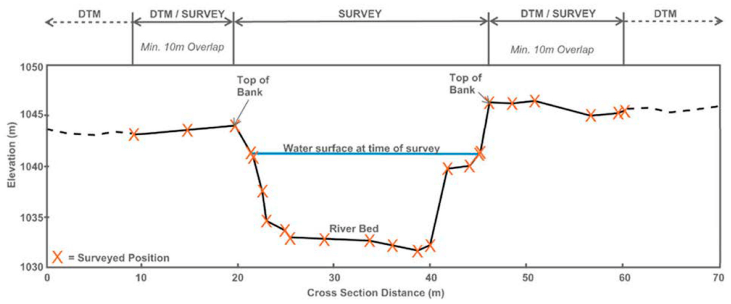
The FHIP guidelines call for high-resolution digital terrain models (DTMs) derived from light detection and ranging (LiDAR) to describe the floodplain topography throughout a flood study area [20]. However, the commonly used LiDAR does not penetrate below the water surface and thus does not collect the bathymetric data needed for standard hydraulic modelling. This includes the collection of bathymetric data along defined cross-sections for 1D modelling (Figure 2) or the collection of sufficient bathymetric data to interpolate a complete channel bed that can be integrated with a floodplain DTM for 2D modelling. LiDAR also does not collect detailed geometries of hydraulic structures such as bridges, culverts, and weirs. Therefore, the accurate survey of stream channels and hydraulic structures remains essential for flood studies.
While advanced remote sensing and LiDAR technology for collecting bathymetric data, as well as watershed characteristics and flood vulnerability information, exist and continue to be developed [21,22], they have technical and practical limitations. For example, they are often more suitable for shallow waterbodies with clear water, which may not be present for all streams in a study area, and steep riverbanks and complex morphologies may affect coverage [23]. For most flood studies, a combination of conventional techniques is still the most accurate and efficient means of collecting data. This can include manual surveys of channel beds by wading in shallow water or the use of acoustic sensors mounted on boats or unmanned surface vehicles (USVs) for deeper water [24]. This type of bathymetric survey work can be time-intensive; therefore, the number and density of cross-sections and/or points to be surveyed needs to be carefully balanced against modelling needs and available resources.
Open-water hydrology assessment is a necessary part of flood studies in Alberta. Regional flood frequency analysis, based on multiple gauges in the region with similar climate and watershed characteristics, can provide regionally appropriate, watershed-specific design values for ungauged watersheds [25].
An important aspect of the open-water hydraulic modelling component is the choice of model dimensionality. More powerful computational resources and high-resolution base data have contributed to the increased use of two-dimensional (2D) hydraulic modelling, where one-dimensional (1D) modelling previously was the default. However, there are additional considerations, including differences in the performance of coupled 1D/2D models and fully 2D models and how field data may improve these models [26]. Site-specific conditions and data availability often inform a decision framework for model choice [27].
The main objective of this paper is to provide insights from two recently completed Alberta flood studies, focusing on technical aspects of the first three FHIP components: (1) survey and base data collection, (2) open-water hydrology assessment, and (3) open-water hydraulic modelling. The Lacombe flood study covers a partly channelized prairie stream network, while the Kinuso flood study covers a laterally dynamic river on a distributary delta.
This paper highlights lessons learned from surveys completed for the two studies, novel hydrology assessments for peak flow estimates of an ungauged stream and hydrograph development for a gauged stream, and advanced numerical modelling techniques for flood mapping. Each study introduced unique challenges, and it is hoped that, by providing key practice-based lessons, this paper can provide examples and guidance for practitioners in the field.
The structure of this paper is as follows. Section 2 introduces the Lacombe and Kinuso flood study areas. Section 3 outlines the survey methods, discussing the challenges encountered and key lessons learned. Section 4 reviews the hydrology assessments undertaken, and Section 5 discusses the hydraulic modelling approaches adopted for the two studies. Section 6 provides practical comparative synthesis and modelling decision guidance, and Section 7 summarizes the conclusions and recommendations.

2. Study Areas

2.1. Lacombe Flood Study

The City of Lacombe (Lacombe hereafter) is in South-Central Alberta, approximately 170 km north of Calgary and 25 km north of Red Deer. Canadian Climate Normals (the average climatic conditions over the period 1991–2020) for Red Deer indicate that temperatures peak in July, with a daily average of 16.2 °C, and reach their minimum in January, with a daily average of −11.6 °C. Total monthly precipitation peaks in June with an average of 97.7 mm and is the lowest in February with an average of 11.9 mm. The average annual total precipitation is 482.6 mm [28].
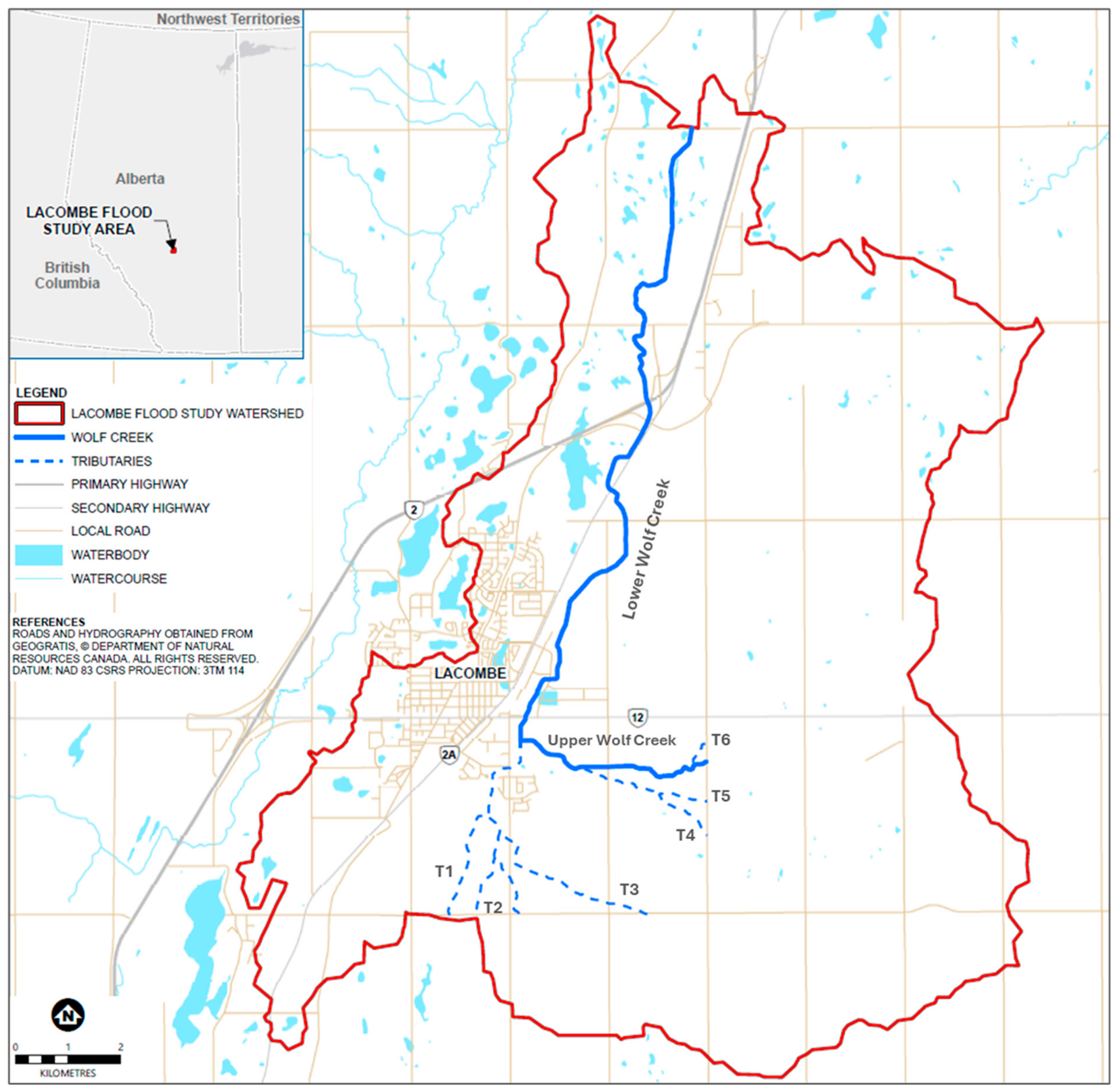
The primary stream in the community is Wolf Creek, the prairie headwaters of which are located southeast of Lacombe. The average slope of the watershed is approximately 2.3% and most of the creek is perennial; however, the tributaries drain into the creek only intermittently. The watershed area of Wolf Creek within the flood study area is 125 km2. Figure 3 illustrates the study stream reaches and contributing watershed area. Wolf Creek was partially channelized in the past, like many streams in agricultural areas, and flows in a general northerly direction through most of the study area. The study includes six unnamed tributaries (Tributaries 1 to 6), all of which join each other or Wolf Creek upstream of Lacombe. Several of the tributaries are considered ephemeral streams and are poorly defined at their origins. The length of the Wolf Creek study reach is approximately 17 km, and the combined length of the tributary study reaches is approximately 14 km. There are no Water Survey Canada (WSC) hydrometric gauge stations on Wolf Creek or its tributaries, and no surveyed high-water marks (HWMs) from past floods are available. Most of the past floods reported in Lacombe were localized urban flooding and not from Wolf Creek or its tributaries.

2.2. Kinuso Flood Study

The Hamlet of Kinuso (Kinuso hereafter) is in North-Central Alberta, approximately 300 km northwest of Edmonton on the south side of Lesser Slave Lake (LSL), approximately 48 km west of the community of Slave Lake. Canadian Climate Normals (1991–2020) for Slave Lake indicate that temperatures peak in July, with a daily average of 16.4 °C, and reach their minimum in January, with a daily average of −13.3 °C. Total monthly precipitation peaks in June with an average of 77.1 mm and is the lowest in March with an average of 12.7 mm. The average total annual precipitation is 422.1 mm [28].
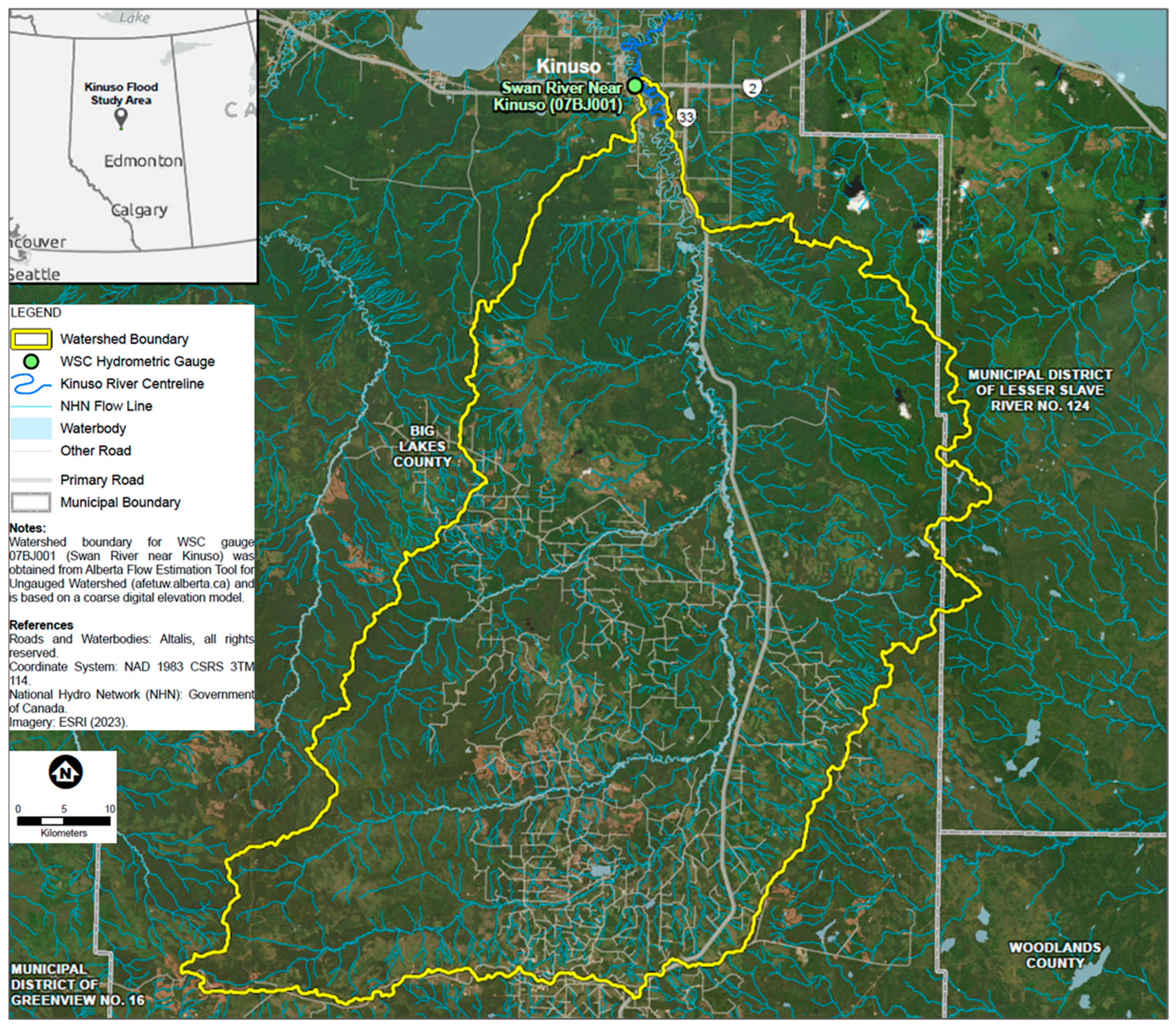
The primary stream in the community is the Swan River, the headwaters of which are in the Swan Hills. Figure 4 shows the study location and the Swan River watershed area at the WSC hydrometric gauge station Swan River near Kinuso (07BJ001). Within the study area around Kinuso, the Swan River is considered a perched channel within a distributary delta. Ground elevations typically slope away from channel banks, and the floodplain has inactive channels that can direct overbank flow away from the Swan River and towards LSL during a flood. The Swan River has a drainage area of approximately 1900 km2 [30] at Kinuso and flows in a northerly direction to its mouth at Swan Point on LSL beyond the study area. The length of the Swan River study reach is approximately 24 km. The average channel width is approximately 35 m, and the overall reach-average channel slope is 0.0005 m/m. The many oxbow lakes and meander scars within the study area provide evidence of the river’s near-constant lateral movement. Surveyed high-water marks (HWMs) are available for floods in 1979, 1982, 1983, 1986, 1988, 2011, 2018, and 2024.

3. Survey and Base Data Collection

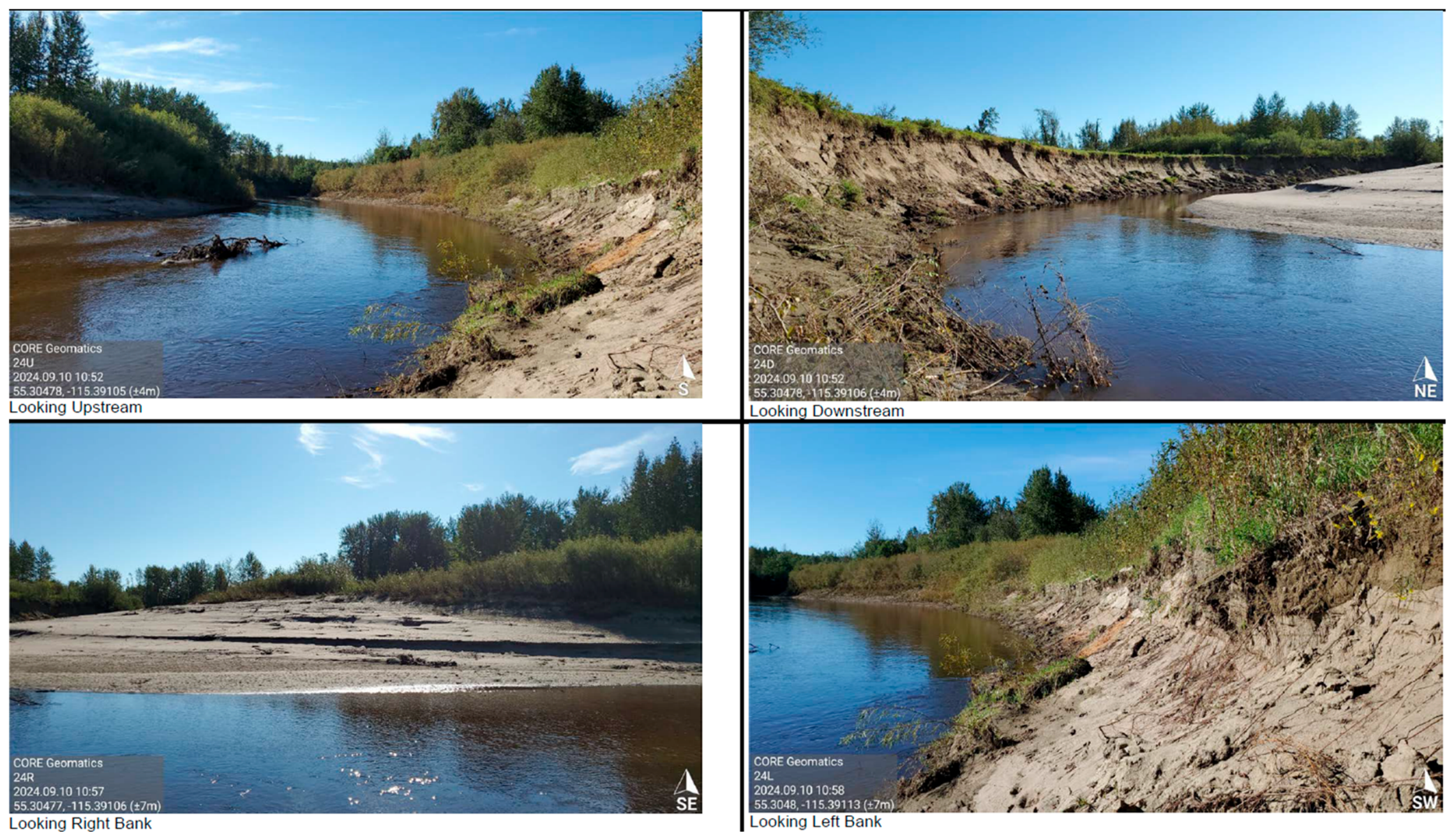
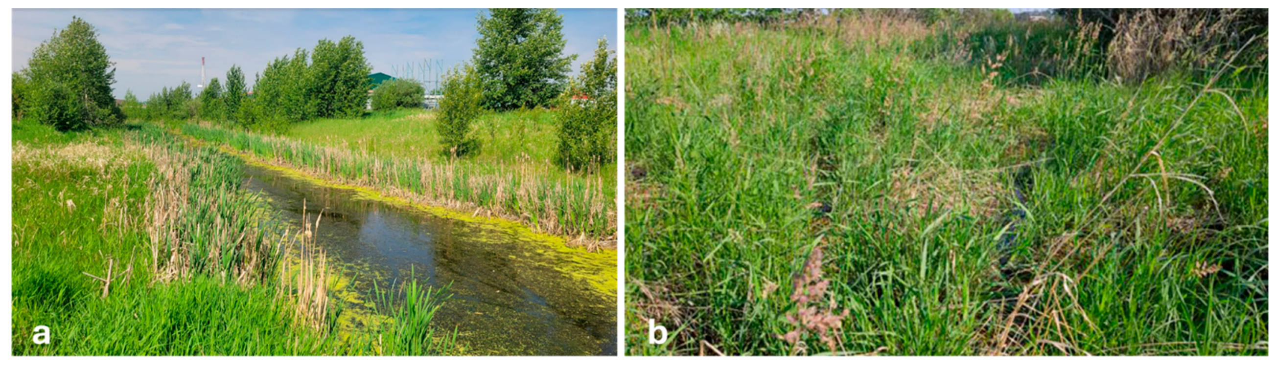
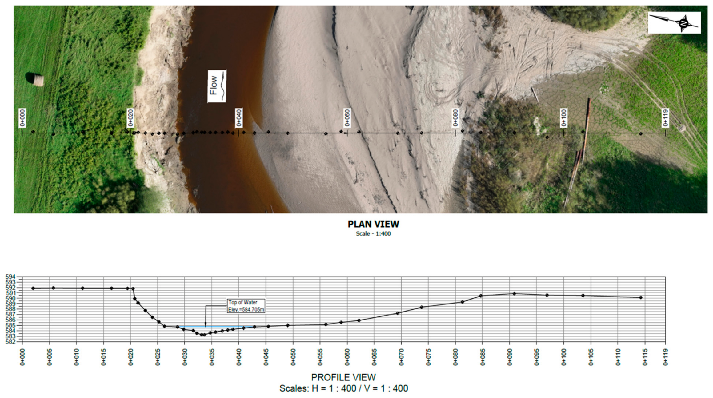
Using an RTK-enabled Trimble R10 survey-grade GNSS receiver, providing centimeter-level horizontal and vertical accuracy [34,35], we collected precise three-dimensional coordinates for each cross-section. This high-precision equipment allowed us to accurately measure both ground elevations and submerged channel bed elevations at each cross-section, with all data georeferenced to the established Alberta Survey Control Monuments (ASCM). Figure 5 and Figure 6 show the riverine conditions during the surveys, and Figure 7 shows a cross-section profile.
Portions of Wolf Creek were channelized in the early 1980s [36]. The average channel width of Wolf Creek is approximately 2 m to 4 m upstream of its major tributary confluence (defined as upper Wolf Creek) and approximately 6 m to 8 m downstream of the confluence (defined as lower Wolf Creek). The average channel slopes along the upper and lower reaches of Wolf Creek are 0.0007 m/m and 0.005 m/m, respectively. Several of the tributaries are ephemeral (i.e., only conveying flow in snowmelt periods or during storm events). Not all were active during the site visit, and all are poorly defined at their origins. Figure 5 shows the typical condition of Wolf Creek and its tributaries.
The Swan River channel is relatively deep and incised, with steep channel banks. Soft sediment dominates and woody debris is common. The river has a high degree of meandering and is perched within the floodplain. Channel characteristics remain relatively constant through the study reach. The average channel width is approximately 35 m, and the average channel slope is 0.0005 m/m. The many oxbow lakes and meander scars within the study area, as well as actively eroding banks, provide evidence of historical and ongoing lateral movement and migration. Figure 6 shows the typical condition of the Swan River within the study reach.
Figure 7 presents a drone-captured plan view of the Swan River and a surveyed cross-section profile at the same location. Note the steep and unstable left bank at this location.
The following sections highlight three lessons learned from the survey and base data collection components of the Lacombe and Kinuso flood studies, as well as a survey data comparison with LiDAR.

3.1. Thinking Ahead

A central lesson from the Lacombe flood study is that forward thinking is essential to project success. Based on information provided in the study initiation phase, it was known that surveyed HWMs from past floods or corresponding WSC-measured peak flows would not be available to support typical hydraulic model calibration. As an alternative, the study team planned to perform discharge measurements during the survey and to collect water levels at each surveyed cross-section. The modelling team could then use this information for a low-flow model’s calibration in the absence of any other high-flow calibration data.
However, it became obvious during the site visit that Wolf Creek was not carrying any significant flow and that water was mostly stagnant in the sub-reaches with visible or even deep water. To resolve this issue, the survey was scheduled during a rain event when the creek was flowing, so that discharge measurements could be completed. Despite careful planning, the measured discharges were still low, with flows between 0.01 m3/s and 0.3 m3/s. To place this in context, the maximum measured flow was approximately 10% of the calculated 1:2 flood flow for that reach (2.74 m3/s). While flood study model calibration should preferably be based on data from floods or high-flow events, the study found that low-flow calibration can offer alternative insight, especially as an upper threshold for establishing reasonable model roughness for higher flows.
The lesson learned from this experience was that collecting discharge measurements and water levels during the survey can be valuable when high-flow calibration data are not available, but flexibility is needed to ensure that suitable data can be collected.

3.2. Detailed Site Visits

Site visits typically take place at the start of flood studies and provide key project team members with the opportunity to assess the channel and floodplain characteristics and fine-tune the locations, alignment, and extent of the planned cross-sections prior to survey work. While the focus of the surveys was collecting bathymetry, it was also important to survey stream banks and a portion of the overbank area to ensure alignment with the LiDAR-derived DTM, acquired in October 2023 and provided by Alberta Environment and Protected Areas (EPA).
Surveying the banks of the Swan River was particularly challenging. High bank walls were obvious during the site visit, and the bank slopes were 50% in some areas. The site visit was performed on a sunny day with dry soil conditions by water resource engineers with a limited geotechnical background. Unfortunately, the survey campaign coincided with a rain event in the region, and the instability of the clay soil banks made it impossible for the field crew to collect enough survey data to properly characterize the bank portions of the cross-sections during the first survey campaign. A second field campaign was planned for mid-September, shortly before the first expected snowfall and at a time when there could be safety concerns. While the survey was able to be completed safely, if this short window had been missed, it would have been necessary to delay the field campaign until the following spring. This would have resulted in at least a six-month delay to the overall study timeline.
The lesson learned from this experience was to conduct enough reconnaissance to fully understand the channel conditions, including bank stability, to ensure a successful survey. However, because of the variable environmental conditions, it is recommended to include contingency when planning, especially in schedule.

3.3. Floodplain Details

Representative local-scale flood mapping typically requires that major hydraulic structures (e.g., bridges, culverts, weirs) along a study reach are included in hydraulic modelling. This means that a detailed survey of hydraulic structures is also often needed in addition to the collection of available design drawings. Typically, surveys or models of all hydraulic structures within a floodplain are not needed, especially when such structures are not expected to have significant impacts or when flood mapping can be manually adjusted to account for minor hydraulic connections.
The study team carefully developed a preliminary high-level 2D model of the study area, using the U.S. Army Corps of Engineers Hydrologic Engineering Center’s (HEC) River Analysis System (RAS), HEC-RAS, to assess potential flooding in the wider floodplain. The preliminary model showed that a substantial number of hydraulic structures would be affected by extreme flood events, especially within Kinuso. The results were used to identify the key hydraulic structures in the wider floodplain that should be included in the more detailed hydraulic model. This exercise informed survey planning and the collection of critical hydraulic structure survey data.
The lesson learned from this experience was that preliminary 2D modelling using available data can help to identify the floodplain features, including hydraulic structures, that require survey and inclusion in a detailed hydraulic model.

3.4. Survey Accuracy and Comparison to LiDAR

Standard GIS processing tools were used to extract DTM elevation values at each surveyed point location. The DTM elevation values corresponded to the DTM pixel value within which the corresponding survey comparison point resided. The tool used was ArcGIS Pro 3.2 “Extract Multi Values to Points” (Spatial Analyst). The option for “Bilinear Interpolation” was left unselected and there was no interpolation applied; the DTM elevation value was extracted from a single cell. The method for comparison was to assess the difference in elevation between the values extracted from the DTM and the surveyed point elevation values. The differences were found through the subtraction of the surveyed values from the DTM values (DTM elevation−survey elevation).
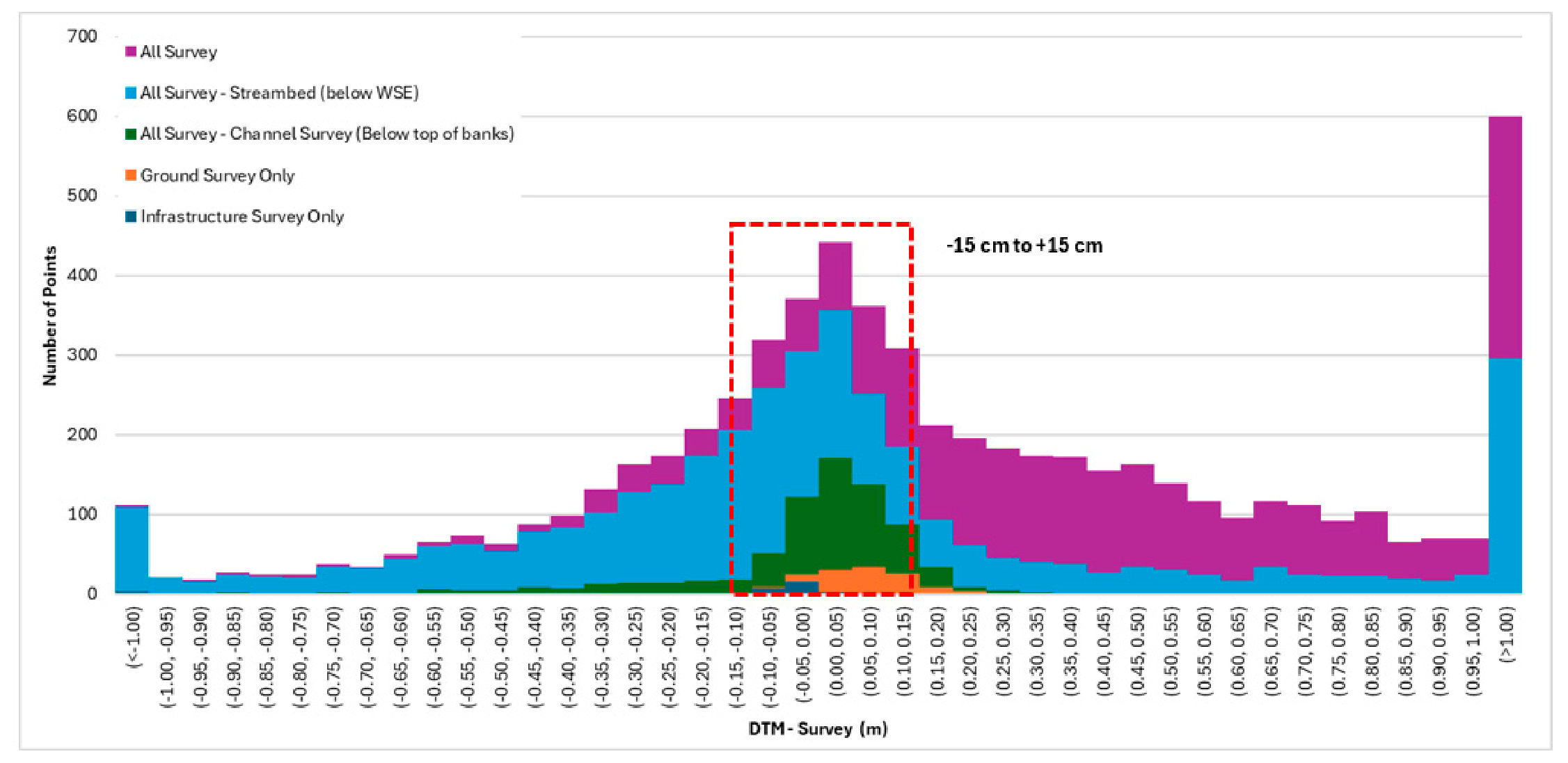
Figure 8 shows the results of the comparison between the surveyed and DTM elevation values as a family of histograms for different classes of survey point data at Kinuso. The range of expected accuracy of the DTM (±15 cm) is provided for comparison. The comparative assessment indicates some discrepancies between the surveyed overbank elevation data and the DTM. It is believed that these discrepancies can be attributed to both steep densely vegetated banks and channel shape changes from large events encountered in 2024. These steep banks can make it difficult to compare directly to LiDAR, as a half-meter cell is likely to cause a large variation in elevation at steep banks (as shown in Figure 7). Additionally, with dense vegetation, LiDAR post-processing may not capture the ground level properly (e.g., post-processing being more favored toward low elevations). The second factor is that the LiDAR device was flown in 2023, while the survey was performed in fall 2024. In this time frame, the river experienced several large flow events that likely altered the channel shape (see Section 5.2.1). It was found that many of the points where the survey was significantly higher were either on depositional areas, such as bars and inside bends, or on the steep banks. With the exclusion of the river survey (i.e., main channel and banks), the ground, LiDAR check, and infrastructure comparison were in good agreement. Therefore, the DTM was found to be suitable for overbank cross-section data extraction and flood mapping purposes.

4. Open-Water Hydrology Assessment

Hydrology assessment to determine the open-water peak flows for the annual exceedance probabilities (AEPs) of 1:2, 1:5, 1:10, 1:20, 1:35, 1:50, 1:75, 1:100, 1:200, 1:350, 1:500, 1:750, and 1:1000, where 1:1000 denotes a flood that has a 0.1% chance of occurring or being exceeded each year, is required for all modelled streams in an Alberta flood study [20]. This typically involves flood frequency analysis (FFA) on flow records, but more sophisticated analyses can be required.

4.1. Lacombe Flood Study

4.1.1. Regional Analysis

Since Wolf Creek and its tributaries are ungauged, a regional FFA was completed using peak annual flow records from the eight WSC stations summarized in Table 1. The stations were selected based on proximity to the study area, the size and slope of their drainage basins, and land cover or topographic characteristics. Regional FFA estimates the annual exceedance probabilities of flood events across multiple watersheds by pooling data from hydrologically similar catchments. This approach is especially useful in areas with limited or no streamflow records, as it leverages the relationships between flood characteristics and physical basin attributes to improve flood risk estimates.
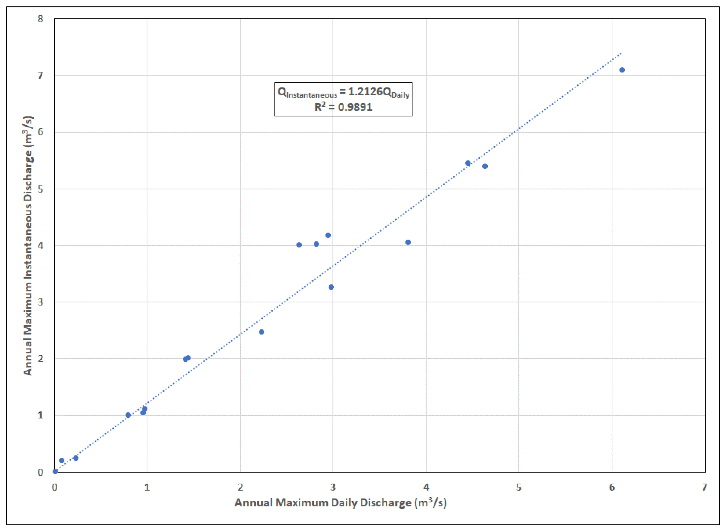
Instantaneous peak flows for some years were missing from the records. In these cases, the available annual instantaneous peak flows were plotted versus the associated annual maximum daily flows, which WSC also provides, to establish relationships to estimate missing annual peak flows. Figure 9 shows the relationship for West Whitemud Creek near Ireton as an example. Linear regression of the available data proved adequate to establish suitable relationships between annual instantaneous peak flows and annual maximum daily flows for all stations.
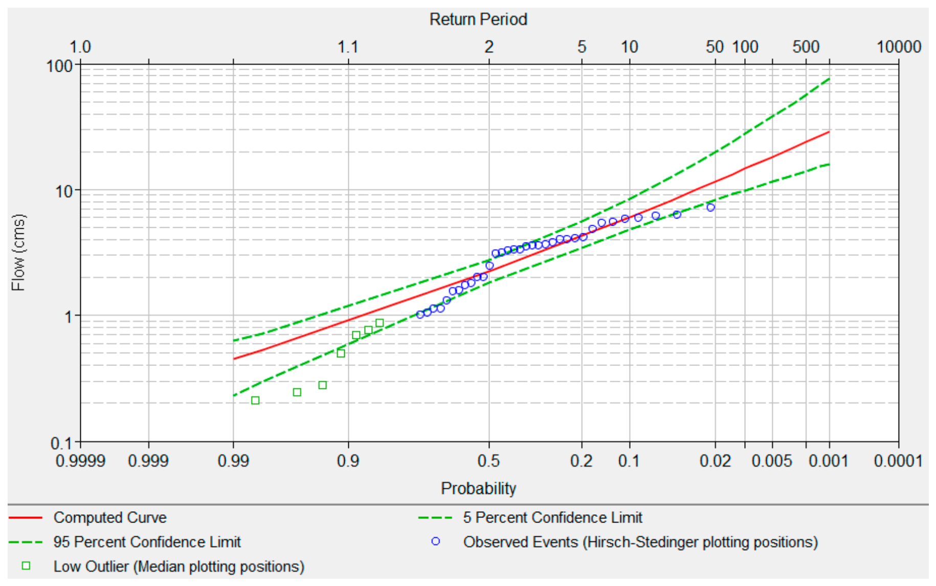
FFA was performed for each station using the resulting annual instantaneous peak flow series. The U.S. Army Corps of Engineers Hydrologic Engineering Center’s (HEC) Statistical Software Package (HEC-SSP version 2.3) was used for FFA [37]. The results based on the Bulletin 17C EMA (Expected Moments Algorithm) method [38], which uses the log-Pearson Type III probability distribution, were adopted for all stations. Bulletin 17C EMA distribution parameters are estimated from the moments of sample data: mean, variance, and skew. The method also includes adjustments for missing years, estimated flow, flow outliers, and historical events by using conditional probability and historical (weighted moments) adjustment, and it characterizes the peak flows as systematic (observed record), historical events, and censored where the peak flow values are missing. The annual peak flow values are presented by flow ranges, with a specified perception threshold for each year. For this study, the maximum peak flow value of the station was used as the perception threshold for the 1964 flow data, which included a substantial number of missing flow values. Bulletin 17C EMA also provides a computed probability distribution with the upper and lower bounds of the selected confidence interval. It is noted that other probability distributions, such as Generalized Extreme Value (GEV) and Gumble, were also tested but not selected and are therefore not included in the paper for the sake of brevity.
Figure 10 presents the FFA results for West Whitemud Creek near Ireton as an example. The plot shows the fitted frequency curve and indicates that most peak flow data points are within the 95% confidence intervals. Comparable results were obtained for all stations selected for the regional FFA.

4.1.2. Regression Analysis

A common approach to projecting regional FFA results to a flood study area is using a simple regression analysis scaled based on the watershed area alone. A more sophisticated approach was taken for the Lacombe flood study. Additional watershed characteristics, including the gross drainage area, effective drainage area, average basin slope, average slope and length of the stream, and storage areas (i.e., the surface areas of ponds and lakes), were also used as predictors and tested to determine whether they were of statistical significance. For instance, if the p-value (a measure of statistical significance) of the predictor was higher than 0.05 (α, significance level), it meant that the predictor was not significant and, in turn, not related to the flood flows (dependent variable). It is noted that the effective drainage area for the Lacombe watershed was adopted from WSC statistics and was checked in GIS for accuracy.
It was found that the average slope and length of the stream were not statistically significant in any of the regression analyses. Storage areas were significant in some, but not all, regression analyses. The average basin slope and storage area were not significant for lower-flood-frequency scenarios (up to a 1:20 flood), but the gross and effective drainage areas were significant for all flood scenarios.
The multiple linear regression analyses were completed using the logarithm base 10 of the data. Equation (1) presents the final form of the regional flood frequency flow equation:
Q T = a X 1 b X 2 c X 3 d
In Equation (1), Q T is the flow in cubic meters per second (m3/s), with the subscript T being the return period of the flood. X 1 , X 2 , and X 3 are the watershed parameters (i.e., gross drainage area, effective drainage area, and average basin slope), and a, b, c, and d are the regression parameters.
After many iterations, it was decided that using both the gross and effective watershed areas had the potential to yield a regression equation that had high goodness of fit but was physically meaningless. The effective drainage area was the main predictor, with a p-value of less than 0.05. In some cases, the p-value for the average basin slope was larger than 0.05, but it was clear that the average basin slope would improve the regression model’s goodness of fit. As a result, the regional equations for flood scenarios included the effective drainage area and average basin slope. This resulted in the use of Equation (2):
Q T = a X 1 b X 2 c
In Equation (2), Q T is the flow in cubic meters per second (m3/s), with the subscript T being the return period of the flood. X 1 and X 2 are the watershed parameters (i.e., effective drainage area and average basin slope), and a, b, and c are the regression parameters. The choice of the effective drainage area over the gross drainage area is further supported by the work of Shook et al., who considered 4000 small basins across the Canadian Prairie region, finding the effective drainage area to be an important hydrologic factor [39].
Finally, the Waskasoo Creek at Red Deer and West Whitemud Creek near Ireton were eliminated from the regional FFA, which significantly improved the results. It is likely that the soil types in the Waskasoo Creek watershed were different, with higher infiltration rates than the other watersheds listed in Table 2 and/or a significantly longer time of concentration due to the larger watershed size; therefore, the calculated peak flows were not in agreement with those of the other watersheds. The West Whitemud Creek peak flow data were not in agreement with those of the other stations, and this could have been due to errors in the drainage area and/or the estimated average basin slope due to the resolution of the available digital DTM used for assessment.
The data from Block Creek near Leedale also appeared to be different from those for the other stations. Unlike in the other streams, most of the Block Creek annual peak flows occurred during warm seasons. However, the characteristics of the peak flows for varying flood frequency scenarios agreed with those for the other streams, and, when eliminating Block Creek from the dataset, the adjusted R2 of Equation (2) improved only slightly. Therefore, Block Creek was used in the regression analyses.
A Lacombe regional flood frequency analysis was previously conducted by the Hydrology Branch of Alberta Environment (Water Resources Management Services, Technical Services Division) in 1992 [40]. They used a different subset of regional gauges and had record lengths from 13 to 27 years, compared to 32 to 42 years in the current study, and they did not use regional regression equations, instead using the average mean annual yield and the average ratio of flood flows to mean annual flows to estimate the flood flows at different locations of Wolf Creek. In 1996, the River Engineering Branch of Alberta Environmental Protection determined that the flood flows estimated in 1992 were too large due to significant ponding in the floodplain [41]. The 1996 study accounted for the storage effects on the peak flows by routing flood flows through the system; therefore, the flood flows were revised. In 2014, MPE Engineering Ltd. (MPE, Calgary, Canada) completed a stormwater management study as part of the Master Drainage Plan for the Wolf Creek and Whelp Brook Watersheds [36]. In that study, MPE conducted a regional flood frequency analysis to estimate flood flows in Wolf Creek for flood events, and they used another subset of regional gauges. MPE used the 3-parameter lognormal probability distributions for flood frequency analysis at all gauges. Finally, MPE used power functions with the watershed area as the independent variable to develop regional equations for the flood flows of the selected AEPs, and the 1:100 AEP flood was slightly smaller than 50% of the one estimated in the 1996 study. The results of the current study show good agreement with those of the 2014 study. These differences indicate the sensitivity of record length and probability distribution function selection in flood frequency analysis, as well as the challenge of defining regionally appropriate stream gauges for regional flood frequency analysis. The differences between the 1992, 1996, 2014, and present studies indicate that regional flood frequency estimates for the ungauged Lacombe watershed remain subject to appreciable uncertainty. This uncertainty reflects differences in gauge selection, record length, distribution fitting, and the representation of storage effects and should be considered when applying the estimated design discharges.
Table 2 lists the parameters and the adjusted R2 of Equation (2) for each flood frequency. Note that the adjusted R2 is between 0.8 and 0.9 for flood frequency scenarios smaller than a 1:20 flood.

4.2. Kinuso Flood Study

4.2.1. Flood Hydrographs

The currently operating WSC hydrometric gauging station, Swan River near Kinuso (07BJ001), is located at Highway 2 Bridge, as shown in Figure 3. The Swan River drainage area at the station is approximately 1900 km2. Annual maximum instantaneous flows are available for 59 years (until 2022). A standard FFA using these data was undertaken in a comparable manner to the Lacombe flood study, as explained in Section 4.1—that is, using Bulletin 17C methods [38]. In 2021, Management and Solution in Environmental Science (MSES) completed a flood risk mapping study supported by the First Nation Adapt Program, Crown Indigenous Relations and Northern Affairs Canada (CIRNAC) for the Swan River First Nation to assess the potential effects of climate change on the risk of flooding in the main reserve and the associated communities [42]. The study used Swan River near Kinuso to perform a flood frequency analysis. MSES used the flow record from 1961 to 2018 using the 2-parameter log-normal distribution. The magnitudes of flood flows with AEPs of 1:5, 1:10, 1:20, and 1:200 were not explicitly reported, but the 1:100 AEP flood event was approximately 5% larger than in the current study. This difference indicates the sensitivity of record length and probability distribution function selection in flood frequency analysis.
The standard and cautious modelling approach outlined in the FHIP guidelines for flood studies in Alberta is to assume steady-state (1D) or quasi-steady-state (2D) flow conditions. However, due to the unique floodplain characteristics of the Swan River at Kinuso, as described in Section 2.2, modelling using an unsteady-state flow assumption was deemed necessary to avoid overestimating flood extents and water levels within the wider floodplain. Inflow hydrographs were thus required for all 13 modelled flood frequency scenarios. Two methods were used to develop candidate hydrographs, which are discussed in detail in the following two sub-sections.

4.2.2. Scaling Pattern Hydrograph (Method 1)

In the first method (herein Method 1), a pattern hydrograph was selected from the largest flood events in the record with the classical shape of a flood hydrograph, i.e., a relatively smooth rising limb, one peak, and a relatively smooth falling limb. In Method 1, the selected pattern hydrograph was scaled to generate hydrographs with peaks equal to the peak flood frequency estimates generated by the FFA.
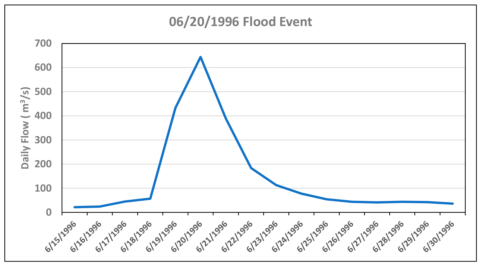
The top three floods of record (1996, 1998, and 2018 floods) were identified as potential candidates for the pattern hydrograph. Among the hydrographs, the hydrograph of the 1996 event was selected as the pattern hydrograph because it had the highest peak flow and had the classical shape of a hydrograph, as shown in Figure 11.
Multiple steps were needed to integrate the FFA results with the pattern hydrograph and develop hydrographs for all 13 flood frequency scenarios. To avoid the overestimation of flood extents, it was important that the hydrographs reflected realistic flood volumes. However, scaling the pattern hydrograph to the peak flood flows estimated from FFA could be subjective, resulting in the overestimation or underestimation of flood volumes.
To support an objective assessment, a critical duration for the pattern hydrograph was estimated, representing a duration that contained most of the flood volume. The duration was measured from the beginning of the rising limb to the inflection point on the falling limb (i.e., where the base flow becomes the main component of the hydrograph). The critical duration of the 1996 flood based on the daily flows plotted in Figure 11 was five days (18 June 1996 to 22 June 1996).
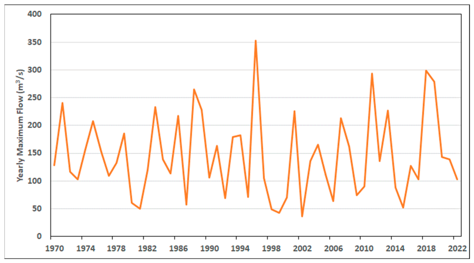
Based on the critical duration assessment, a 5-day moving average flow series was developed from the Swan River near Kinuso gauge daily flows from 1970 to 2022. Data before 1970 were not used because the amount of missing data was not conducive to developing complete 5-day moving averages in this period. A corresponding annual maximum series was subsequently created, as shown in Figure 12. Scaling factors for each flood scenario were calculated by dividing the FFA peak flows by the maximum 5-day moving average flow (351.8 m3/s).
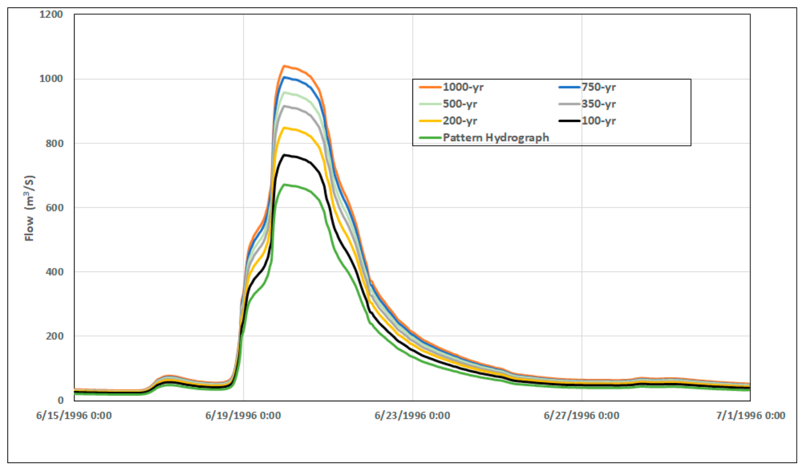
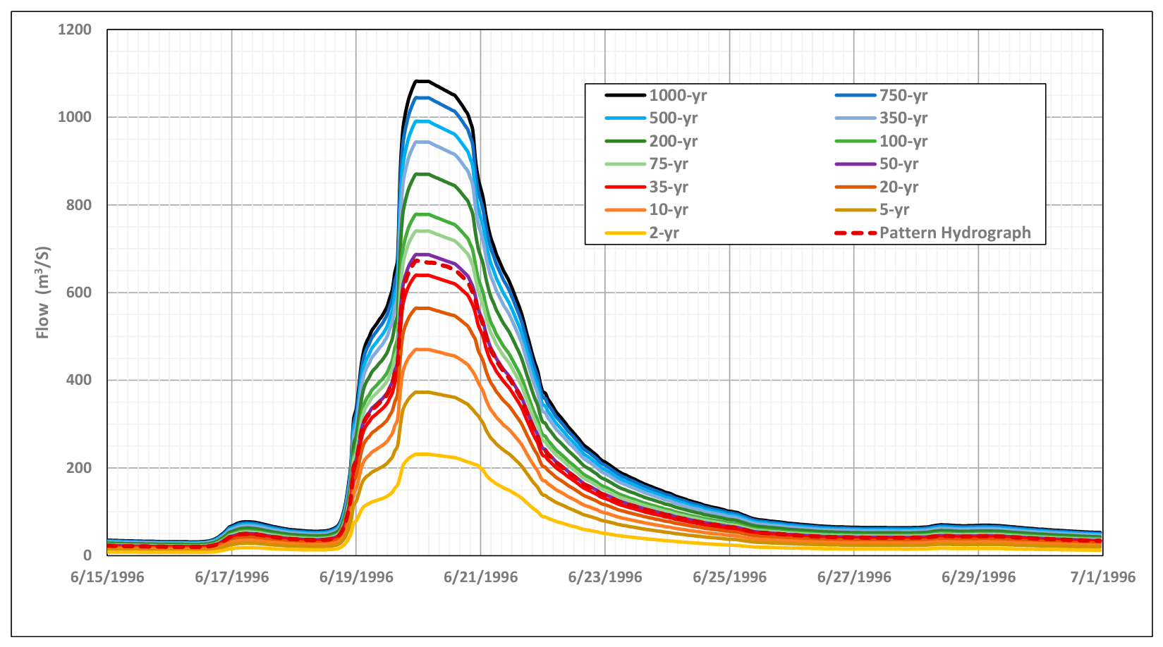
The scaling factors for each flood frequency scenario were applied to the hourly flows of the pattern hydrograph from 15 June 1996 to 30 June 1996 to obtain the set of scaled hydrographs shown in Figure 13.
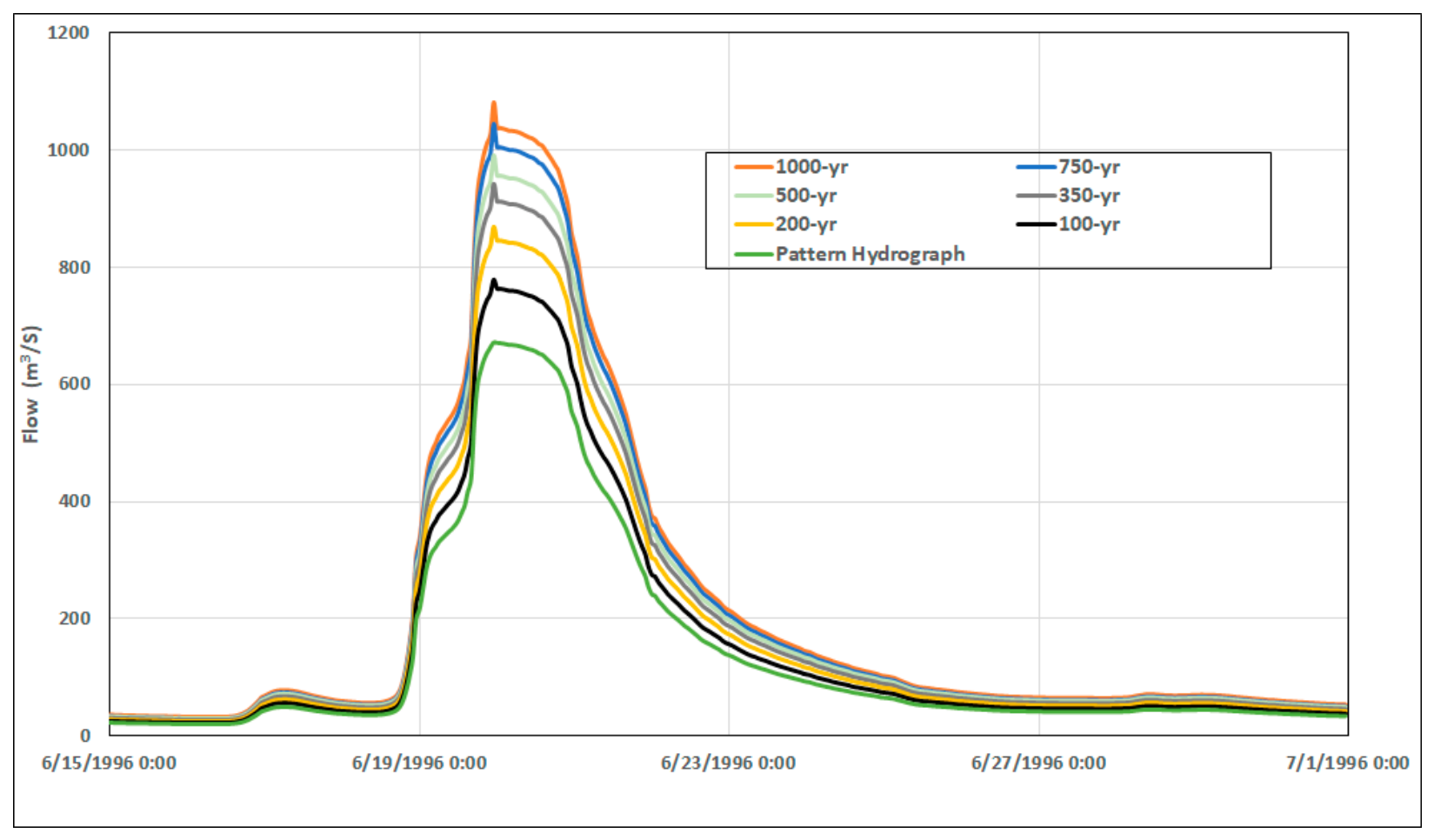
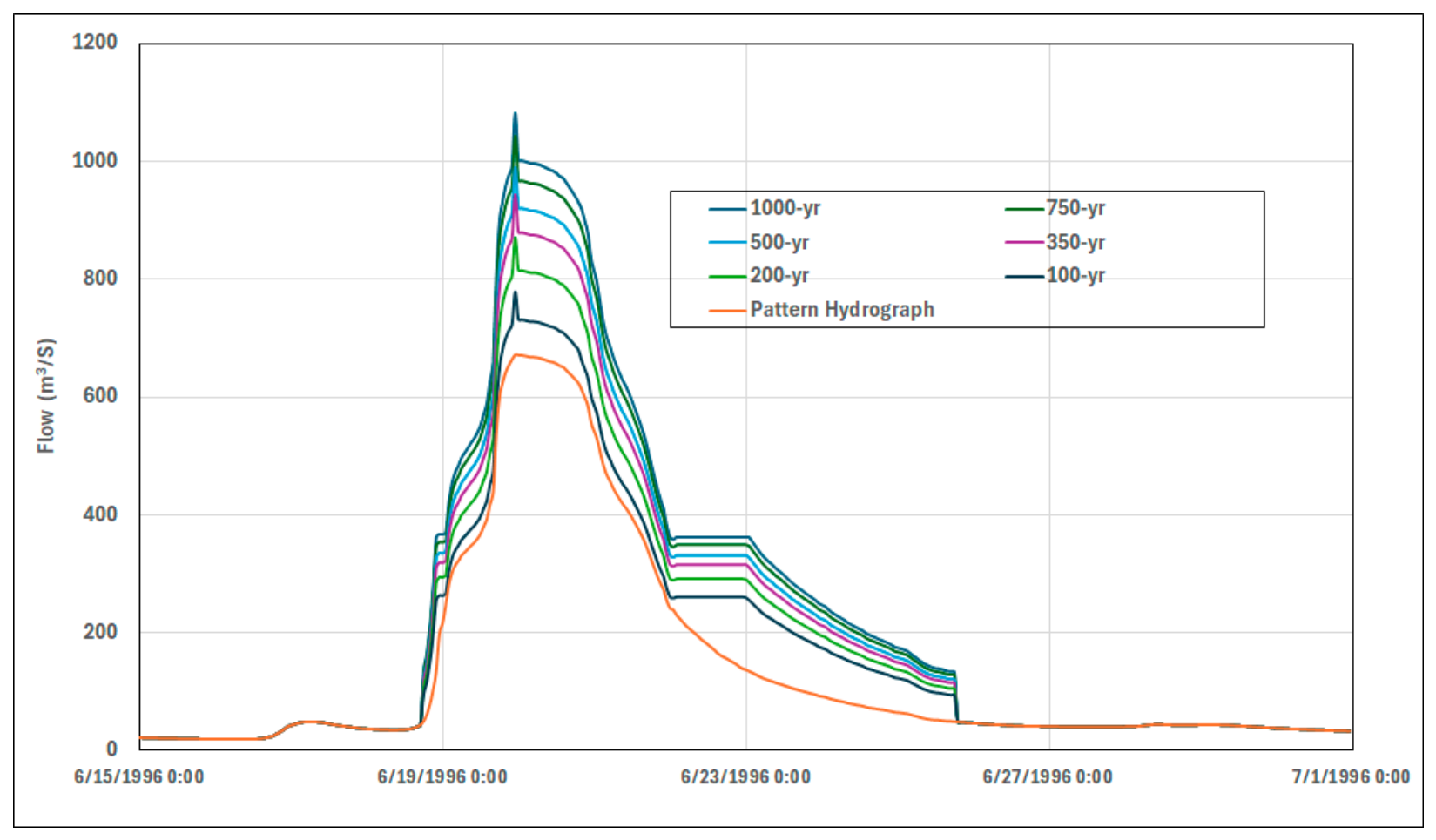
While the scaled hydrographs aligned well with the pattern hydrograph, the peaks did not match those determined from the FFA of the WSC-reported peak flows. This is because the hydrographs were based on a frequency analysis that considered volumes. Adjustments of the scaled hydrographs to force their peaks to match the flow-based FFA peaks are shown in Figure 14. The coarse adjustments are visible as spikes, which are an unrealistic representation of flood hydrographs.
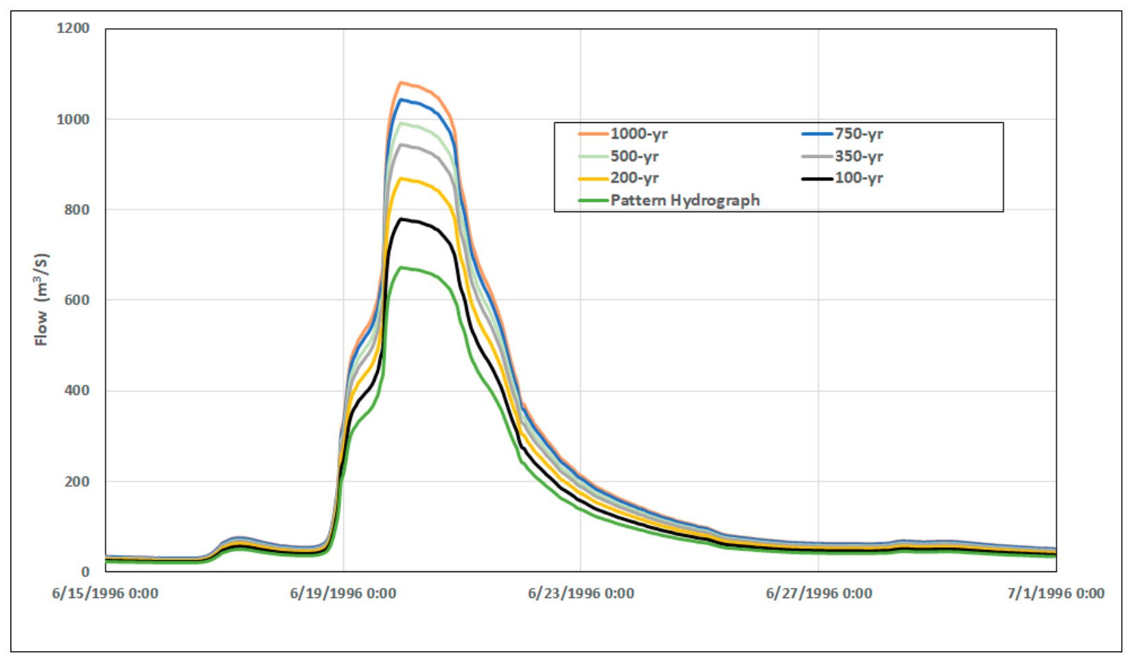
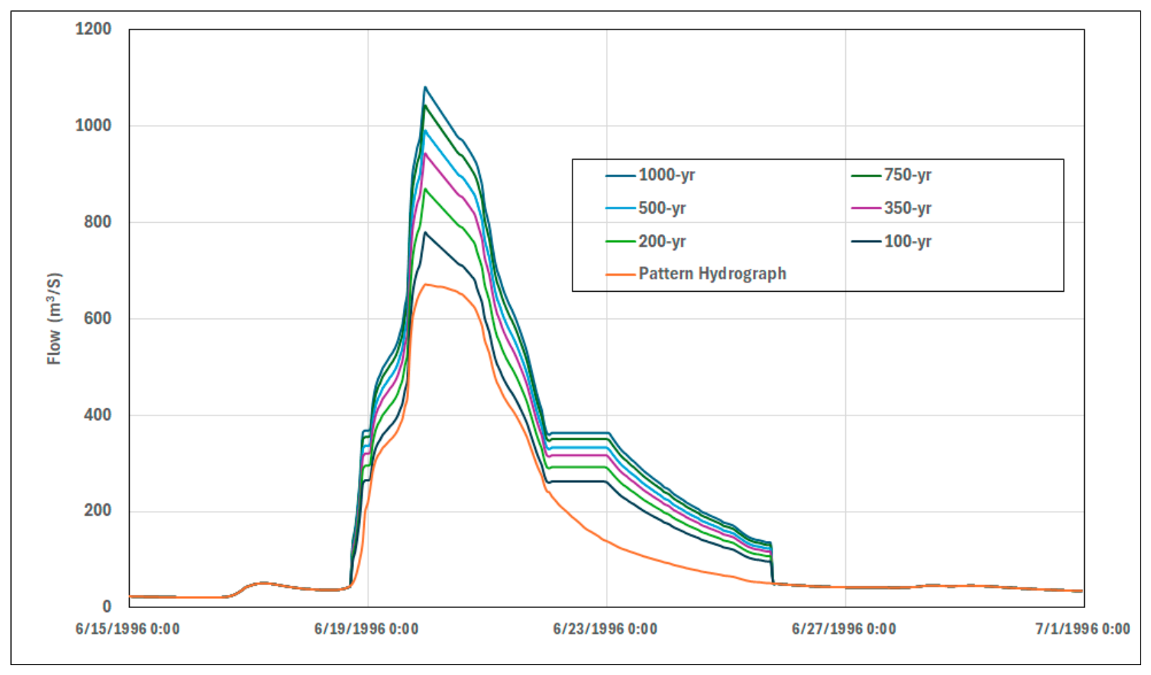
To eliminate the spikes, the hydrographs were smoothed using linear interpolation around the peaks. The resulting smoothed hydrographs are shown in Figure 15.
The resulting smoothed hydrographs are reasonable and justifiable from a technical perspective, but they are based primarily on the pattern hydrograph. It is unlikely that the characteristics of the 1996 flood hydrograph would be exactly replicated for all potential future floods. To reflect this uncertainty and reintroduce a reasonable level of caution consistent with standard FHIP steady-state or quasi-steady-state flow assumptions, one final set of adjustments was made to the Swan River inflow hydrographs. The final adjustment was to sustain the peak flows for six hours and linearly interpolate the flows to a lower flow on the falling limb. This choice was made after looking at other recorded flood hydrographs and trials of sustained peaks of different durations to assess the sensitivity of the 2D model results and preliminary mapping (see Section 5.2.3 for additional details). The final Method 1 hydrographs are shown in Figure 16.

4.2.3. U.S. Army Corps of Engineers Balanced Hydrographs (Method 2)

As an alternative to Method 1, HEC-SSP was used to develop balanced hydrographs, following the general methodology that the U.S. Army Corps of Engineers (USACE) uses in their projects [37]. A balanced hydrograph is a hydrograph that has an equal exceedance probability for all possible critical durations. For this method, a pattern hydrograph like the one in Method 1 was used. In addition, the daily flow data were rearranged using 1-day, 3-day, and 7-day moving averages to develop the annual maximum series of 1-, 3-, and 7-day volumes. Subsequently, frequency analyses were performed on the annual maximum series of 1-, 3-, and 7-day moving average flows. Based on the results, a set of balanced hydrographs was developed by using the pattern hydrograph as a template. As was the case at this stage of Method 1 hydrograph development, and for similar reasons, the peaks did not match those determined from the FFA of the WSC-reported peak flows. Similar adjustments to the balanced hydrographs were made to force their peaks to match the flow-based FFA peaks, as shown in Figure 17. The resulting hydrographs were in general agreement with those developed using Method 1 and shown in Figure 14.
To eliminate the spikes, the hydrographs were smoothed using linear interpolation around the peaks. The results are shown in Figure 18. Given the smooth hydrograph shapes, no further adjustments were made. The resulting balanced hydrographs are similar to those obtained in Method 1. Method 1 and Method 2 differ primarily around the beginning of the rising limbs and towards the end of the falling limbs. The volumes around the peaks are also slightly larger in Method 1 when compared to those in Method 2.
Upon evaluation, it was decided that the flood hydrographs developed using Method 1 were more suitable for modelling and mapping, and it was recommended that they be used as the inflow hydrographs for the 2D modelling of the Swan River.
Lessons learned from the hydrology assessment include the need for flexible and alternative methods for flood frequency analysis because of sparse data—a challenge that is common for local-scale flood studies. In addition, inflow hydrographs for flood frequency scenarios are an important aspect that allows practitioners to make more sophisticated hydraulic modelling choices.

5. Open-Water Hydraulic Modelling

Alberta’s FHIP guidelines provide details on hydraulic modelling best practices for provincial flood studies. Open-water hydraulic modelling using the HEC-RAS modelling platform [43], developed and maintained by the USACE Hydrologic Engineering Center (HEC), is required for provincial flood studies. The platform is freely distributed, non-proprietary, and USACE-maintained. The HEC-RAS platform can be used for 1D, 2D, and coupled 1D/2D modelling. Using HEC-RAS allows stakeholders to leverage hydraulic models for other purposes, including operational flood risk assessment and evaluating local projects and flood mitigation plans.
Prior to the 2022 revision of the FHIP technical guidelines, all provincial flood studies were conducted using 1D modelling techniques. The 2022 revision officially permitted the application of primary 2D hydraulic modelling [20]. Therefore, a combination of 2D and coupled 1D/2D modelling was used for the Lacombe flood study, while full 2D modelling was used for the Kinuso flood study. Discussions around the rationale for the selected modelling approaches, as well as model setup and calibration, are presented and discussed in the following.

5.1. Lacombe Flood Study Model

Based on the site visit, a review of the ground conditions and the DTM, and the collected survey data, a coupled 1D/2D modelling approach for the well-defined lower Wolf Creek study reach was selected. Based on the poorly defined channels in some areas and the potential for flow interaction between tributaries, a full 2D modelling approach was selected for the upper Wolf Creek study reach and for six tributaries.
A preliminary 1D model was constructed for the study area in the initial stages of model development to inform the final modelling method. This model used clipped cross-sections (i.e., only including the main channel) along Wolf Creek, where there was a high degree of confidence in the coupled 1D/2D method. In the upper Wolf Creek reach and along all tributaries, cross-sections spanning the floodplain were created. This was performed to investigate whether a 1D model would be appropriate for the poorly defined channels in the upper reaches. One-dimensional modelling of the upper reaches was found unsuitable as the DTM elevations were not only higher than the corresponding surveyed elevations along the main channels (as expected) but also higher than the water levels for low flood events (e.g., for the 1:2, 1:5, and 1:10 floods).
Compared to the 1D modelling approach, the coupled 1D/2D and full 2D modelling approaches adopted for the Lacombe flood study offered the following benefits:
  • A 1D component maintains the benefits of a 1D model, including the accurate simulation of the main channel hydraulics in the well-defined lower Wolf Creek reach;
  • Two-dimensional modelling in a domain that includes significant areas of flat agricultural floodplain can reduce the uncertainty associated with defining representative cross-section alignments and the selection of appropriate ineffective flow areas;
  • The complicated flow paths in the floodplain containing the upper Wolf Creek and tributary reaches are better represented with 2D modelling;
  • Two-dimensional modelling reduces the risk of profiles crossing at locations where the ineffective flow areas required for 1D modelling would be activated when flood control structures, levees, or roads are overtopped.

5.1.1. Model Setup

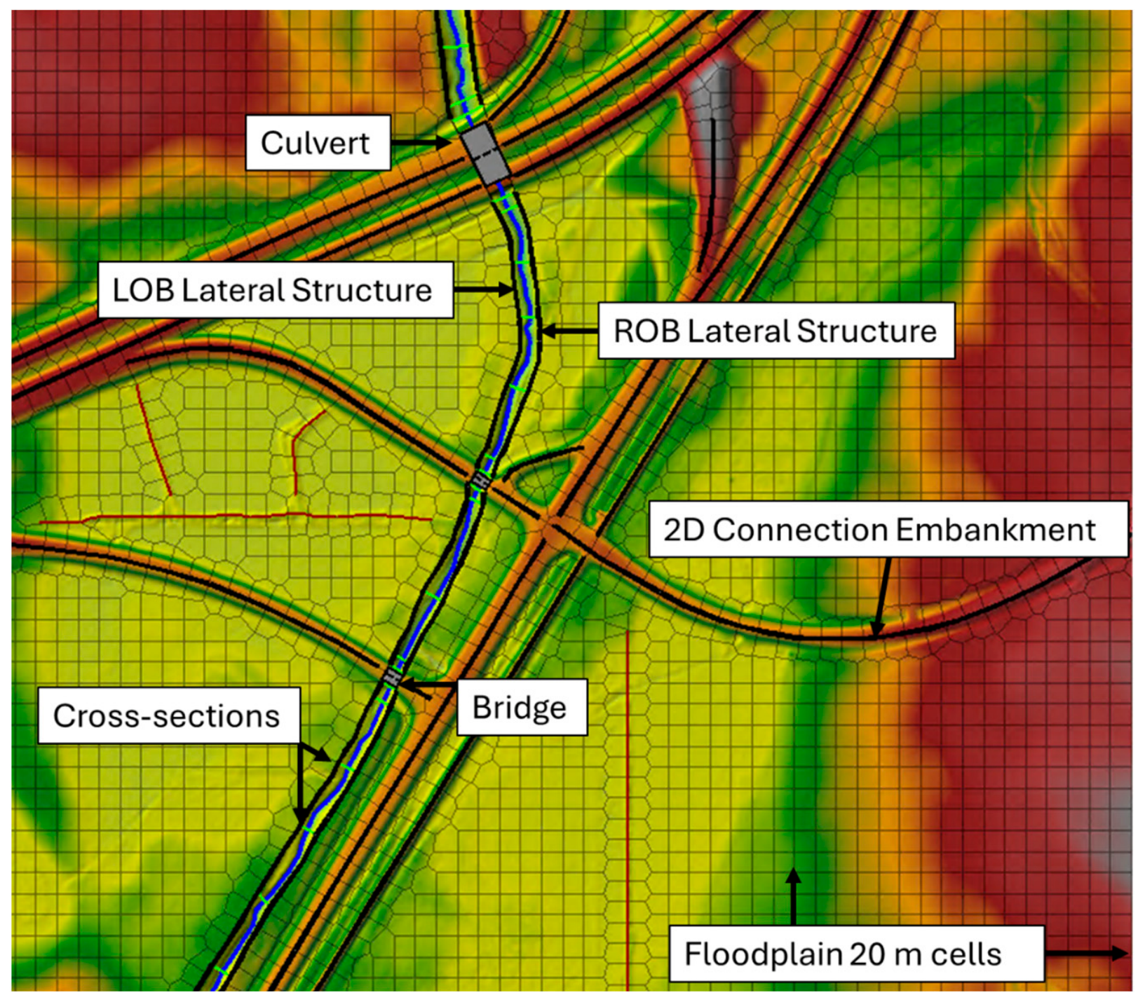
In total, 19 km of the study reach was modelled within a fully 2D domain, and 12 km was modelled within a coupled 1D/2D domain. Figure 19 provides a detailed view along a portion of lower Wolf Creek in the coupled 1D/2D model domain.

5.1.2. Digital Terrain Model

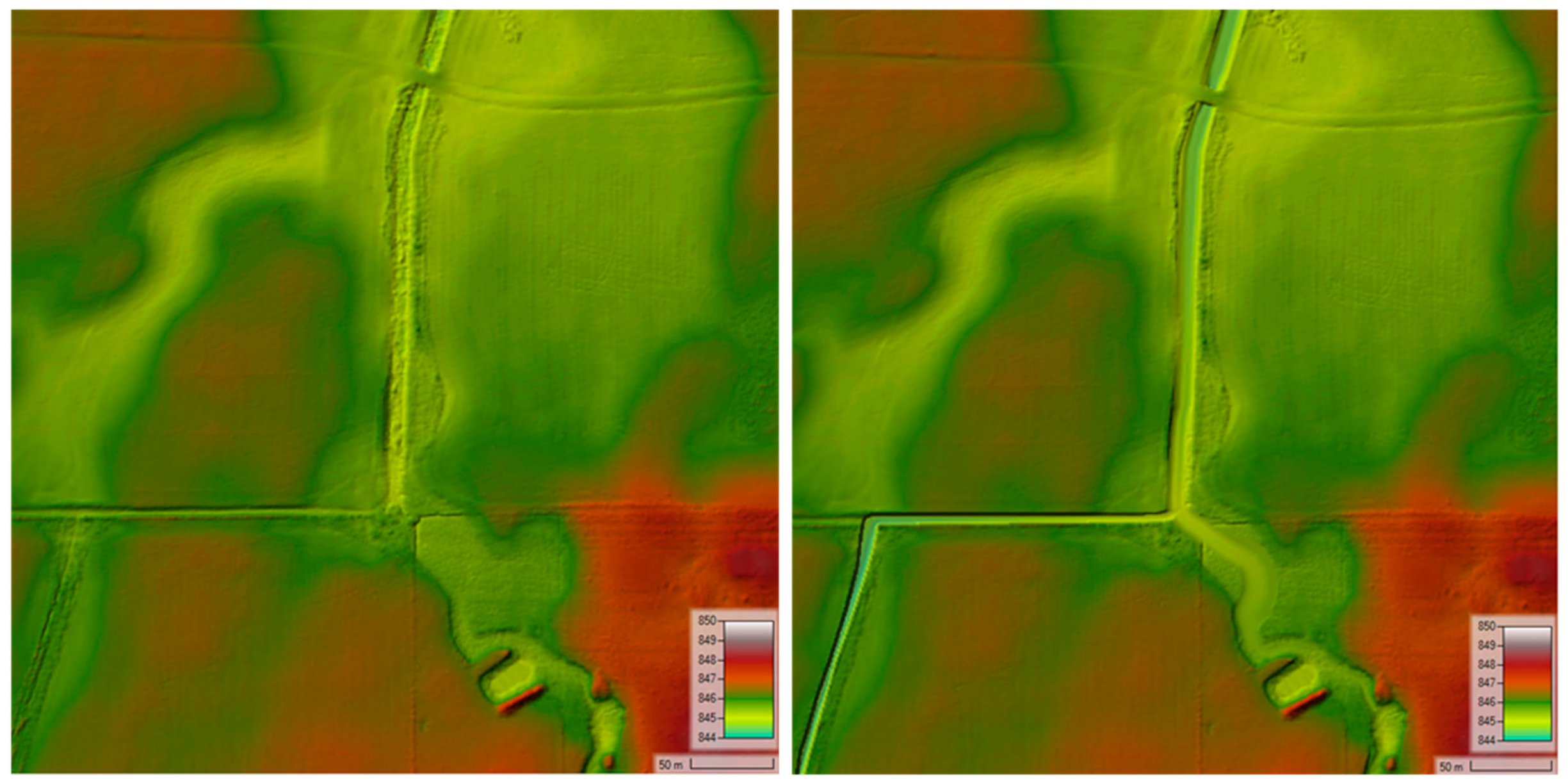
For the fully 2D domain (i.e., upper Wolf Creek and the tributaries), a composite DTM combining the surveyed cross-sections (for the main channel) and high-resolution DTM (for the floodplain) was created by necessity. The composite surface eliminated the issue of dry regions when the water levels in the main channel are lower than in the DTM, and it was used for flood mapping. Note that the model cross-sections along the lower Wolf Creek reach used the survey points and were not extracted from this composite surface. However, the composite surface was used for mapping to eliminate dry regions when the simulated main channel levels were lower than in the DTM.
A GIS tool was developed that used the surveyed cross-sections to create interpolated intermediate cross-sections. The tool helped to define the distances between the interpolated cross-sections, allowing for the accurate definition of the required channel bathymetry. Cross-section data were used to create a triangulated irregular network (TIN) within defined bank lines, which was then converted to a channel bathymetric DTM. This raster was mosaicked into the study DTM to create a composite surface. Figure 20 shows an example of such a composite DTM. The composite DTM has a resolution of 0.5 m.

5.1.3. Boundary Conditions

HEC-RAS models that include 2D domains require the specification of boundary conditions at all open and internal boundaries. The open boundaries of the Lacombe flood study hydraulic model are listed below:
  • Inflows at the upstream model boundaries of the upper Wolf Creek reach and all tributary reaches;
  • Normal flow conditions (with an estimated energy slope of 0.03%) at three downstream model boundaries of the lower Wolf Creek reach (one for the left floodplain, one for the main channel, one for the right floodplain);
  • Local point inflows to resolve flow accumulation issues that deviate from the hydrology assessment or are caused by unsteady flow modelling.

5.1.4. Numerical Details

Based on the modelling approach selected (as explained above), the HEC-RAS model required the use of an unsteady-state numerical solver. Note that inflows are modelled using a quasi-steady-state flow assumption, where inflow hydrographs increase until they reach the peak flow estimated in the hydrology assessment, after which the inflows are kept constant for the duration of simulation. The most robust solver available was selected for computation: SWE-ELM, which stands for Shallow Water Equations with a Eulerian–Lagrangian Method. The SWE equation solution method is more momentum-conservative but may require smaller time steps and longer run times (compared to the default diffusion wave solver). The SWE-ELM solver in HEC-RAS uses a combination of the continuity and momentum equations from the St. Venant equations, which are discretized using a semi-Lagrangian approach for the acceleration terms and a mixed finite-difference/finite-volume method for the overall solution [43]. The continuity equation enforces mass conservation, while the momentum equation is a full momentum-based set that includes gravity, pressure, and acceleration terms.
The continuity equation ensures that mass is conserved within each control volume or grid cell and, for incompressible fluids like water, is expressed as
𝜕 h 𝜕 t + 𝜕 q x 𝜕 x + 𝜕 q y 𝜕 y = S
and the momentum equation in two-dimensional form is expressed as
𝜕 u 𝜕 t + u 𝜕 u 𝜕 x + v 𝜕 u 𝜕 y = g 𝜕 z s 𝜕 x + 1 h . υ t h u + f c ν g S f x
𝜕 v 𝜕 t + u 𝜕 v 𝜕 x + v 𝜕 v 𝜕 y = g 𝜕 z s 𝜕 y + 1 h . υ t h v + f c u g S f y
where h is the water depth; t is the time step; qx and qy are the flow rates in the x and y directions, respectively; S is a source/sink term; u and v are the depth-averaged horizontal velocities in the x and y directions; g is gravitational acceleration; zs is the water surface elevation; νt is the turbulent eddy viscosity coefficient; fc is the Coriolis parameter; and Sfx and Sfy are the friction slopes in the x and y directions, as defined by Manning’s equation.
In general, this solver captures changes in water surfaces and velocities at and around hydraulic structures, piers/abutments, and tight contractions and expansions better than the other solvers in HEC-RAS.
The 2D computational mesh has 94,342 cells, and it was refined to balance accuracy and computational costs. Modelling started with a uniform mesh of 3 m × 3 m but was refined for smaller channels to ensure mesh independence in the water level results and model accuracy and coarsened in the floodplain. It is noted that the 2D mesh initially covered a larger area; however, to reduce the run time, the model domain was cut (in an iterative process) to reduce the total number of cells. The final model domain contained the 1:1000 flood extent with a general buffer of approximately 100 m.
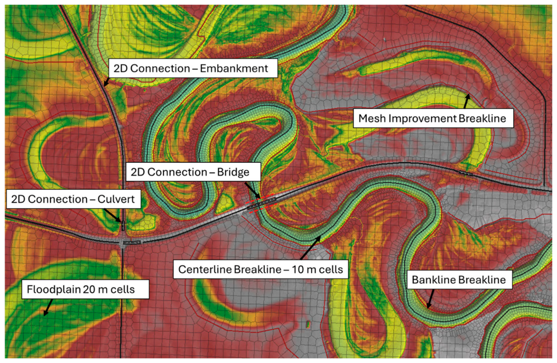
Lateral structures were used to connect the 1D cross-sections of lower Wolf Creek to the left and right 2D floodplain domains. Breaklines were used in the 2D domain as needed, including 2D connections for hydraulic structures and as weirs on major roads. Table 3 summarizes the Lacombe flood study model details.
HEC-RAS multiplies the absolute difference in velocity head by a coefficient to account for the effect of flow contraction or expansion on the energy balance between successive cross-sections. The coefficients range from 0.10 for gradual transitions to 0.80 for abrupt transitions [44]. These coefficients are applied in a steady-state simulation at all cross-sections. In addition to the 1D domain, expansion and contraction coefficients are used at 2D bridge internal cross-sections. The default coefficients of 0.3 and 0.5 were used in 2D domain bridges (i.e., default values). Weirs were incorporated in the fully 2D domain on large roads, highways, and railways. A weir coefficient of 1.45 was assigned for all hydraulic structure embankments. A weir coefficient of 0.2 was used for the lateral structures, which resemble overland flow rather than a typical broad-crested weir.

5.1.5. Model Calibration

The initial channel roughness used for Wolf Creek during model construction was based on site visit observations of the channel conditions and engineering experience. The roughness values were then calibrated based on the water level and discharge data measured on 23 June 2023. Three discharges were measured on Wolf Creek: at river stations 15,500 m, 4236 m, and 395 m with flows of 0.011 m3/s, 0.134 m3/s, and 0.291 m3/s, respectively. As noted in Section 3.1, the maximum measured flow was approximately 10% of the calculated 1:2 flood flow for that reach (2.74 m3/s). As discussed previously, low-flow model calibration is valuable to gain confidence in model parameters, especially the main channel roughness values, when high-flow calibration data are not available. However, the uncertainty associated with extrapolating low-flow calibration to extreme flood conditions is a shortcoming that should be considered in such situations.
Using the 2023 discharge measurements, the main channel roughness (i.e., Manning’s n) along Wolf Creek was calibrated to 0.035 for low-flow conditions. A Manning’s n value of 0.04 was used for the upper section (from river station 16,500 m to 15,930 m), where the channel is less defined. The model calibration process for low flow involved multiple iterations to adjust the model parameter values, conduct simulations, and compare the simulated water levels to the surveyed water levels. The simulated and surveyed levels differed by −0.01 m on average, with a range of −0.011 m to +0.09 m.
Discharges were not measured for the tributaries because no flow was observed during the field survey; thus, no corresponding low-flow calibration was performed. The main channel roughness (i.e., Manning’s n) for all tributaries was set as 0.04, in consideration of the stream bed and bank material, vegetation cover on the banks, site observations, and prior experience. There are no HWMs or flood imagery available for Wolf Creek or its tributaries within the study area; therefore, no high-flow calibration could be completed.

5.1.6. Model Sensitivity Analysis

In the absence of HWMs for high-flow model calibration, a model sensitivity analysis was conducted to evaluate the effects of changing the model roughness values and downstream boundary conditions on the simulated water levels. The 100-year flood event was used for model sensitivity analysis. The sensitivity analysis results were used to quantify the level of uncertainty associated with the simulated flood levels along the study reach of Wolf Creek.
The analysis of model sensitivity to Manning’s n involved the following two sets of Manning’s n values for the main channels and floodplains and one set of downstream boundary conditions. The results of the sensitivity analysis indicate the following:
  • The uncertainty in the simulated flood levels, on average, is within a range of −0.03 to +0.04 m for lower Wolf Creek and ±0.02 m for upper Wolf Creek, based on the differences in the simulated flood levels for a ±10% change to the base channel Manning’s n value only.
  • The uncertainty in the simulated flood levels, on average, is within a range of ±0.00 m for lower and upper Wolf Creek, based on the differences in the simulated flood levels for a ±10% change to the base floodplain Manning’s n values only.
  • A ±20% change to the energy slope at the downstream boundary influences the simulated flood levels by ±0.06 m for approximately 0.3 km upstream of the downstream boundary.

5.2. Kinuso Flood Study Model

As noted in Section 1, Section 3 and Section 4.2, full 2D modelling was selected for the Kinuso flood study due to the unique Swan River channel and floodplain characteristics, and the model was run using inflow hydrographs and an unsteady-state flow assumption. The 2D model setup and composite DTM creation followed the approaches described in Section 5.1 for the Lacombe flood study model; thus, common details are not repeated in this section.

5.2.1. Model Setup

The 2D computational mesh had 128,740 cells. Modelling started with a uniform coarse mesh of 30 m × 30 m for the floodplain. It was reduced to 10 m × 10 m for the river channel to ensure mesh independency in the water level results and the accuracy of the model. Mesh independency testing was completed and it was determined that a finer mesh of 7 m × 7 m would not significantly change the model results (i.e., a change of less than 2% in water levels and velocities). Given the computational cost of a finer mesh, the 10 m × 10 m refinement was selected. Three principal breaklines along the Swan River centreline and left and right banks were added, and mesh refinements were imposed to improve the modelling of side channels and topographic controls. Moreover, 2D connections were used for hydraulic structures and along major roads, railways, and flood berms in the floodplain. Figure 21 provides a detailed view of a portion of the 2D model domain. Table 4 summarizes the Kinuso flood study model details. An advanced time step control was used to reduce the time step from 4 s to 2 s during the peak of the hydrograph.
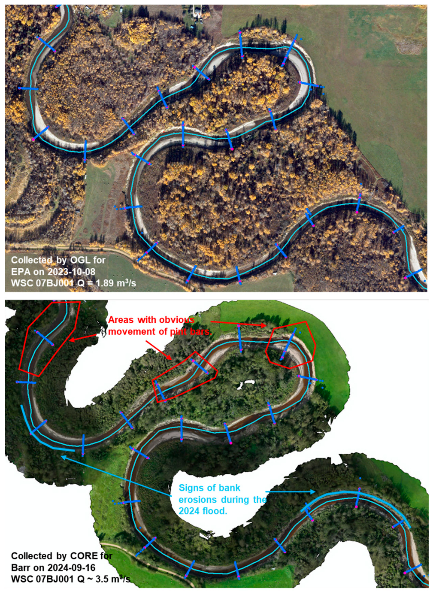
It is also noted that the Swan River is highly mobile, both laterally and with regard to sediment transport. Figure 22 illustrates changes to the Swan River from river station 18,500 m to river station 15,500 m over a year that were caused by flooding on 27 July 2024. The flood peak was approximately 477 m3/s, which roughly corresponds to a 1:10 flood. This illustrates the importance of using up-to-date DTMs and highlights that flood mapping can often only best represent conditions at a snapshot in time. To continuously update the survey and associated modelling, mapping and reporting would be unrealistic. The projection of future channel forms is too complex and would introduce unacceptable uncertainty. This emphasizes the importance of the regular review of past studies and the selection of updates.

5.2.2. Model Calibration

Low-flow discharge measurements were collected during the Swan River survey even though HWMs from past floods were available. Therefore, both low-flow and high-flow calibrations were completed for the Kinuso flood study model. In addition to these calibrations, the model was validated against the WSC rating curve and flood photos (latter two not discussed in this paper).
Low-Flow Calibration
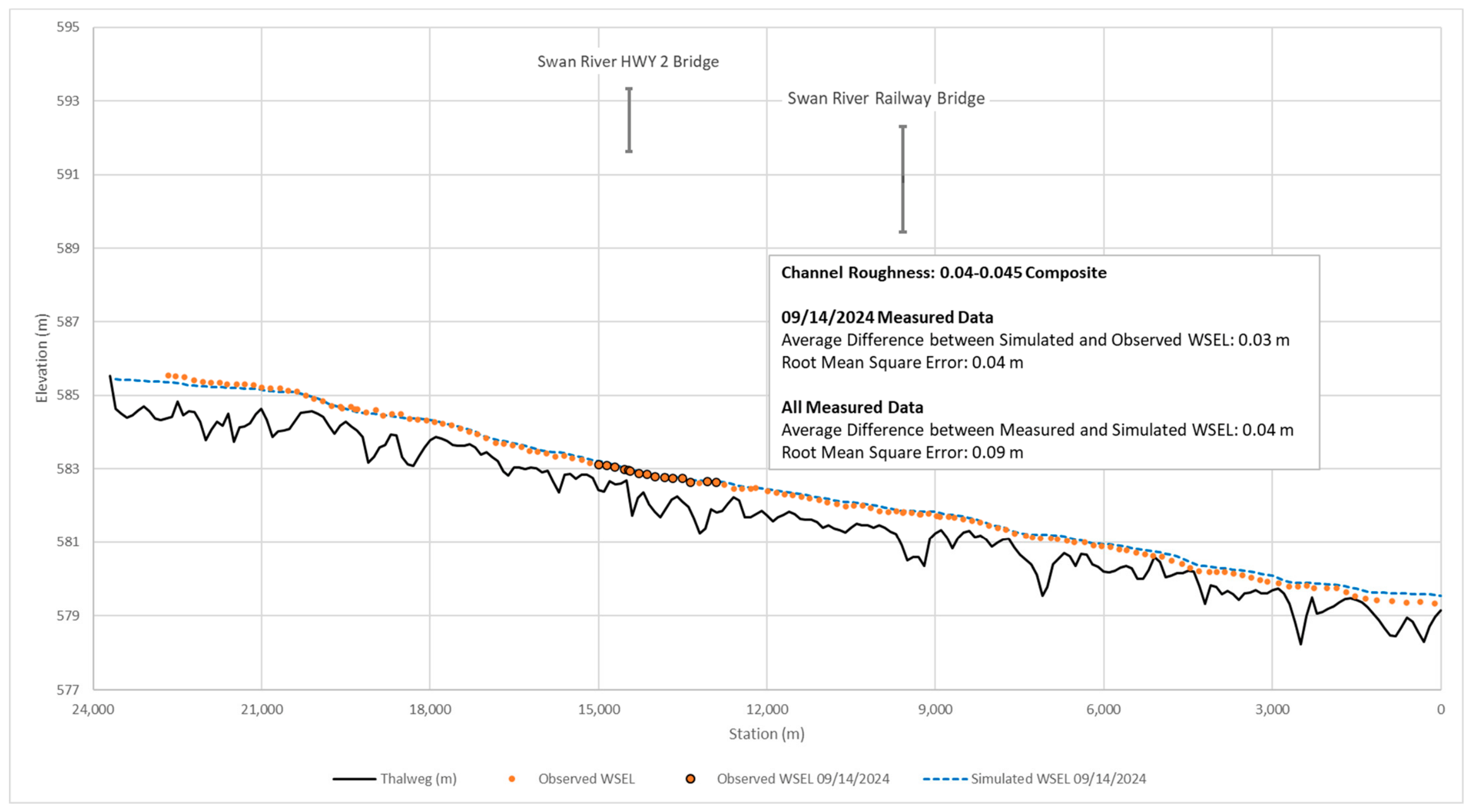
The initial channel roughness used for the Swan River during model construction was based on site visit observations of the channel conditions and engineering experience. The roughness values were then calibrated based on the water level and discharge data measured on 14 and 16 September 2024. Two discharges were measured on the Swan River: at river stations 14,400 m and 7300 m with flows of 3.67 m3/s and 3.22 m3/s, respectively.
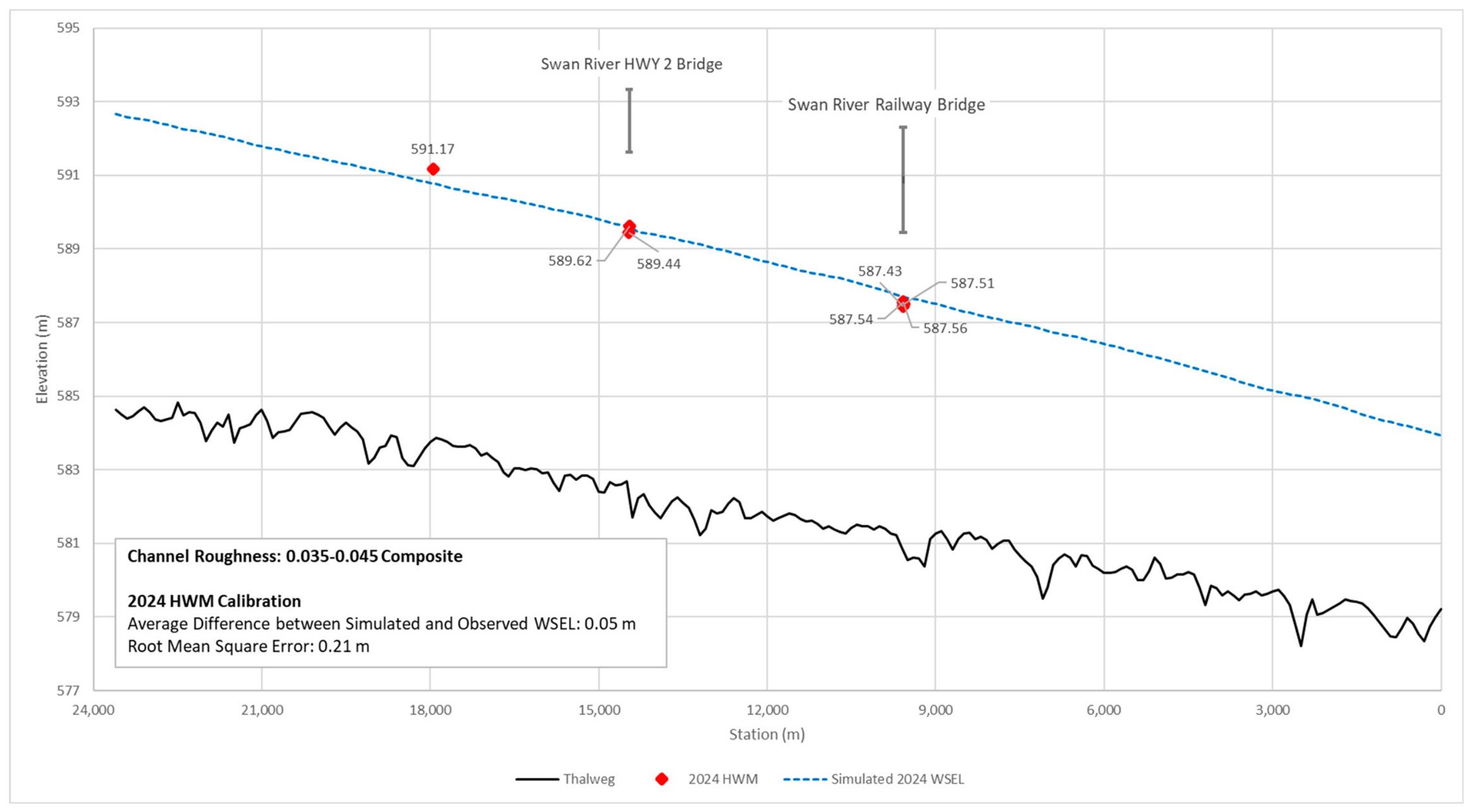
In the process of calibration, it was decided that a composite two-layer channel roughness layer would represent the river system more accurately. The Swan River has tall banks that are often heavily vegetated, which contrasts sharply with the smoother sediments making up the channel bottom. Therefore, assigning two roughness values for these areas increased the accuracy of the model. Figure 23 presents the calibration profile for the 14 September 2024 measurements. The simulated and surveyed levels differed by +0.04 m and 0.00 m for 14 and 16 September 2024, respectively. Based on low-flow calibration, the composite main channel roughness (i.e., Manning’s n) was set to 0.04 for the channel bed and to 0.045 for the channel banks.
A model sensitivity analysis was completed for Kinuso, similarly to Lacombe, as described in Section 5.1.6, but is not discussed here for the sake of brevity.
High-Flow Calibration
The model was further calibrated for high-flow conditions based on HWMs collected for the eight past floods. The high-flow calibration results, summarized in Table 5, show strong performance for more recent floods, with the underestimation for older floods attributable to bed degradation, channel migration, and cutoff formation. The calibration profile for the 2024 flood (with a peak flow of 477 m3/s) is plotted in Figure 24.

5.2.3. Inflow Hydrograph Selection Discussion

As described in Section 4.2, the Kinuso flood study model uses inflow hydrographs and an unsteady-state flow assumption—an approach used for the first time for Alberta flood studies. Before the final hydrographs were recommended, tests were performed using the hydraulic model to confirm that the approach was suitable and assess the sensitivity of the flood extents for different sustained peak flow durations. The analysis included modelling the hourly 1:100 and 1:1000 flood hydrographs presented in Figure 15 with four sustained peak flow durations: 1 h, 3 h, 6 h, and with the peak flow sustained to the end of the simulation period (i.e., the quasi-steady-state flow assumption).
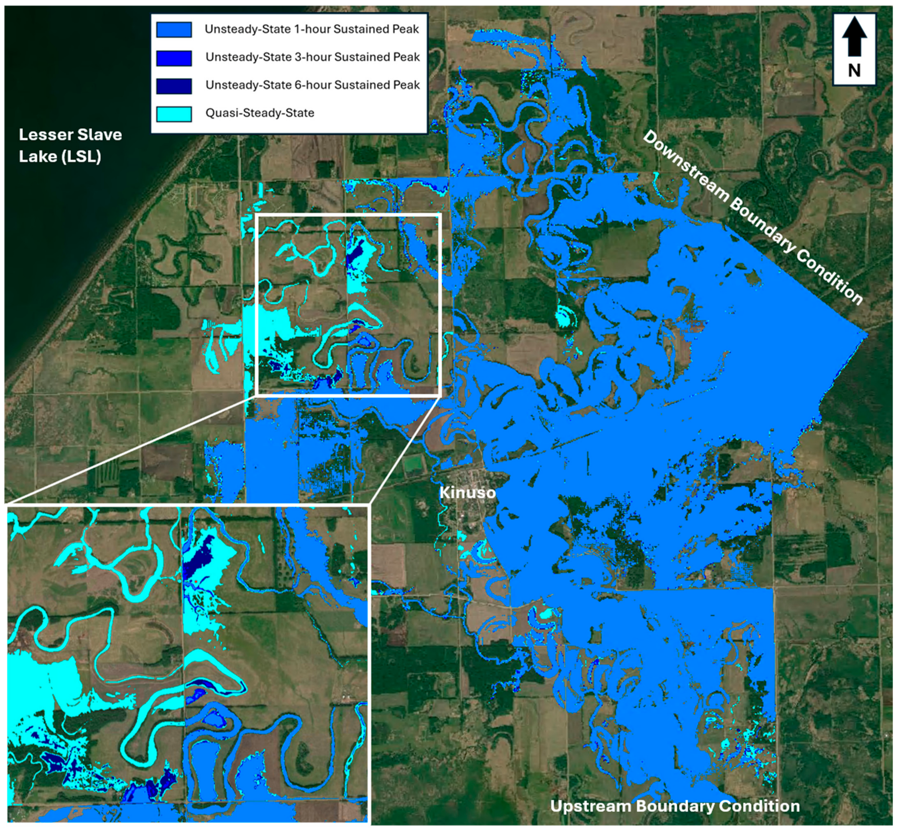
As expected, the quasi-steady-state hydrographs produced the largest flood extents. The flood extents based on the 6 h sustained peak hydrographs were only slightly smaller but more realistic in the far floodplain, as shown in Figure 25. The flood extents from all unsteady hydrograph variations did not differ enough to obtain definitive conclusions about underestimation or overestimation. Reviewing the range of results confirmed that using an unsteady-state flow assumption was reasonable for this study area and model setup, and it was decided to finalize the inflow hydrographs with a 6 h sustained peak.
Lessons learned include that, in ungauged reaches lacking high-water marks, opportunistic low-flow discharge and water level surveys can provide a defensible channel roughness calibration option, thereby improving the numerical stability and reducing parameter compensation in subsequent flood frequency simulations. In addition, thoughtful hydraulic modelling, underpinned by site visits and hydrologic modelling, supports a clear decision framework for dimensionality selection. Finally, the study reach characteristics for flood mapping may influence the choice of steady-state versus unsteady-state (using hydrographs) model simulations.

6. Comparative Synthesis and Modelling Decision Guidance

Taken together, the Lacombe and Kinuso case studies show that the technical pathway for local-scale flood hazard identification must be matched to the geomorphic setting, data availability, and the dominant mechanism of floodplain inundation. For field surveys, the Lacombe study area was comparatively more accessible because Wolf Creek and several tributaries were shallow, weakly incised, or intermittently dry; however, this same intermittency limited opportunities for discharge measurement and low-flow calibration, because some tributaries were inactive during the initial survey. In contrast, the Swan River at Kinuso offered a clearly defined channel but a substantially more difficult and hazardous survey environment due to its depth, steep and locally unstable banks, and weather-sensitive access. Across both settings, the common lesson is that LiDAR-derived topography alone is insufficient where channel conveyance controls flood levels; detailed reconnaissance, explicit safety planning, and the integration of targeted bathymetric and bank survey data with the floodplain terrain are therefore essential best practices for cold-region local-scale flood studies.
The hydrologic and hydraulic analyses likewise required different but complementary solutions. In Lacombe, the ungauged, multi-tributary system required regional flood frequency analysis and the assignment of design inflows at multiple flow change locations. Because the selected model used coupled 1D/2D routing over a relatively flat prairie floodplain, continuity had to be preserved by distributing local inflows in a manner consistent with sub-watershed drainage patterns and topographic controls, thereby avoiding unrealistic localized inundation from overly concentrated floodplain inflows. In Kinuso, the presence of a long hydrometric record simplified flood frequency estimation, but steady or quasi-steady assumptions were not representative because the perched, tortuously meandering Swan River spills into a broad deltaic floodplain where storage, attenuation, and multi-path routing materially influence the stage and extent. Representative hydrographs for 13 flood scenarios and unsteady fully 2D simulations were therefore required. These paired results suggest a practical modelling framework: 1D modelling is most applicable where the channel is laterally confined, flow paths are predominantly longitudinal, and lateral storage is limited; coupled 1D/2D modelling is preferable where the main channel remains well defined but overbank routing, tributary interaction, or hydraulic structures govern floodplain behavior; and full 2D modelling is warranted where channels are poorly defined or highly laterally connected, or where distributed storage, flow split, and infrastructure controls dominate inundation. Similarly, steady or quasi-steady simulations are generally suitable when hydrograph timing has a limited influence on the mapped water levels, whereas unsteady simulations should be adopted when floodplain storage, attenuation, and delayed return flow materially affect flood levels and extents, as in laterally connected deltaic environments.

7. Conclusions

This paper provides engineering insights and key practice-based lessons from two recently completed flood hazard identification projects in Alberta, Canada: the Lacombe flood study, which focused on Wolf Creek and six tributaries (a relatively small prairie stream system with partially channelized and poorly defined channels), and the Kinuso flood study, which focused on the Swan River (a relatively large, laterally mobile river with a wide floodplain perched within a distributary delta). The paired case studies show that the primary sources of uncertainty for detailed, local-scale flood mapping include channel terrain fidelity (bathymetry and bank definition); the sparseness of data; the representation of flood hydrographs where floodplain storage and attenuation materially influence simulated flood extents; and appropriate hydraulic modelling approaches (1D, 2D, or coupled 1D/2D) consistent with the governing flow paths and floodplain connectivity.
Survey and base data collection insights confirmed that LiDAR-derived DTMs alone are insufficient where channel conveyance controls the stage, because the water surface masks bed elevations and steep banks can be mischaracterized. This aligns with the findings from a recent review [23], which documented that environmental and geometric conditions, including steep banks, turbidity, and vegetation, can compromise topo-bathymetric LiDAR coverage. Our direct RTK GNSS survey approach provides a reliable alternative when these conditions limit remote sensing methods. Experiences with the Kinuso flood study further highlighted that field logistics are a technical control on data quality: steep, cohesive banks became inaccessible under rainfall, directly limiting the number and distribution of bathymetric and bank points that could be surveyed. Accordingly, engineering-led reconnaissance that explicitly evaluates bank materials, access risks, and seasonality (including snow onset constraints in northern regions) should be treated as an integral part of study design, with explicit schedule contingency.
Hydrology assessment insights showed that regional flood frequency analysis, an integral component in dealing with sparse data, can be improved by testing physically meaningful basin descriptors beyond drainage areas. For the Lacombe flood study, evaluating the gross versus effective drainage area, basin slope, and storage metrics and screening predictors based on statistical significance improved the interpretability and reduced the extrapolation risk for ungauged tributaries. For the Kinuso flood study and its unique channel and floodplain characteristics, the development and use of inflow hydrographs was a technical advancement versus steady-state or quasi-steady-state flow assumptions. The volume-consistent scaling of a representative pattern hydrograph using a critical-duration moving-average frequency analysis, followed by peak shape refinement, produced hydrographs that better reflected the routing behavior in a large watershed and resulted in more realistic flood mapping outcomes.
Experiences with the Lacombe flood study showed that, in ungauged reaches lacking high-water marks, opportunistic low-flow discharge and water level surveys can provide a defensible channel roughness calibration option, improving the numerical stability and reducing parameter compensation in subsequent flood frequency simulations.
Thoughtful hydraulic modelling, underpinned by site visits and hydrologic modelling, supports a clear decision framework for dimensionality selection. In the Lacombe flood study, 2D modelling improved flood extent delineation for poorly defined prairie streams versus standard 1D modelling; in contrast, a coupled 1D/2D modelling approach remained advantageous for the well-confined lower Wolf Creek study reach because it preserves 1D conveyance in the main channel while resolving complex overbank routing and flow split behavior in the 2D domain. The full 2D modelling approach taken for the Kinuso flood study was necessary to resolve complicated multi-path floodplain flow patterns, backwater interactions with linear infrastructure, and distributed storage effects.

Author Contributions

Conceptualization, H.K.G., P.O., O.M., C.F., T.M., M.D. and P.O.; methodology, H.K.G., P.O., O.M., C.F., T.M., M.D. and P.O.; investigation, H.K.G., P.O., O.M., C.F., T.M., M.D. and P.O.; writing—original draft preparation, H.K.G.; writing—review and editing, H.K.G., P.O., O.M., C.F., T.M., M.D. and P.O. All authors have read and agreed to the published version of the manuscript.

Funding

The Lacombe and Kinuso flood studies were completed by Barr Engineering for the Government of Alberta under the provincial Flood Hazard Identification Program, which aims to enhance public safety and reduce future flood damage through the identification of river and flood hazards. The studies were co-funded by the Government of Canada through the federal Flood Hazard Identification and Mapping Program (23RSD919 & 24RSD894).

Data Availability Statement

The original contributions presented in this study are included in the article. Further inquiries can be directed to the corresponding author.

Acknowledgments

The authors would like to thank Karen Ryberg, Moges Wagena, Kinda Chakas, Eddie Anderson, Emily Cristobal, Carmen Orosz, Mike Miller, and Shayne MacDonald for their support.

Conflicts of Interest

Authors Hossein Kheirkhah Gildeh, Paul Orban, Omid Mohseni, Christian Frias, and Tom MacDonald were employed by the Barr Engineering Company. The remaining authors declare that the research was conducted in the absence of any commercial or financial relationships that could be construed as a potential conflict of interest.

Abbreviations

The following abbreviations are used in this manuscript:
AEPAnnual exceedance probability
ASCMAlberta Survey Control Monuments
CIRNACCrown Indigenous Relations and Northern Affairs Canada
DTMDigital terrain model
EMAExpected moments algorithm
FDRPFlood Damage Reduction Program
FFAFlood frequency analysis
FHIP(Alberta’s) Flood Hazard Identification Program
FHIMPFlood Hazard Identification and Mapping Program
GNSSGlobal navigation satellite system
HECHydrologic Engineering Center
HWMHigh-water mark
NDMPNational Disaster Mitigation Program
LiDARLight detection and ranging
LSLLesser Slave Lake
RMSERoot mean square error
RTKReal-time kinematic
SWE-ELMShallow Water Equations with a Eulerian–Lagrangian Method
TINTriangulated irregular network
USACEU.S. Army Corps of Engineers
USVUnmanned surface vehicle
WSCWater Survey Canada
NHNNational Hydro Network

References

  1. Hirabayashi, Y.; Mahendran, R.; Koirala, S. Global Flood Risk Under Climate Change. Nat. Clim. Change 2013, 3, 816–821. [Google Scholar] [CrossRef]
  2. Lulham, N.; Warren, F.J.; Walsh, K.A.; Szwarc, J. Canada in a Changing Climate: Synthesis Report; Government of Canada: Ottawa, ON, Canada, 2023; 71p. [Google Scholar]
  3. Grenier, M.; Boudreault, J.; Raymond, S.; Boudreault, M. Projected Seasonal Flooding in Canada under Climate Change with Statistical and Machine Learning. J. Hydrol. Reg. Stud. 2024, 53, 101754. [Google Scholar] [CrossRef]
  4. Simonovic, S.; Perry, B. Local Scale Current and Projected Future Total Flood Hazard Mapping for Canada—Literature Review. J. Flood Risk Manag. 2025, 18, e70091. [Google Scholar] [CrossRef]
  5. Public Safety Canada. Government of Canada Funds Flood Mitigation Project in Ontario. Public Safety Canada. 2019. Available online: https://www.canada.ca/en/public-safety-canada/news/2019/05/government-of-canada-funds-flood-mitigation-project-in-ontario.html (accessed on 11 June 2026).
  6. Westra, S.; Fowler, H.; Evans, J.; Alexander, L.; Berg, P.; Johnson, F.; Kendon, E.; Lenderink, G.; Roberts, N. Future changes to the intensity and frequency of short-duration extreme rainfall. Rev. Geophys. 2014, 52, 522–555. [Google Scholar] [CrossRef]
  7. Shiomi, Y.; Seto, Y.; Uno, N. Model for location of medical facility and evaluation of vulnerability and accessibility of road network. Transp. Res. Rec. 2011, 2234, 41–48. [Google Scholar] [CrossRef]
  8. Albano, R.; Sole, A.; Adamowski, J.; Mancusi, L. A GIS-based model to estimate flood consequences and the degree of accessibility and operability of strategic emergency response structures in urban areas. Nat. Hazards Earth Syst. Sci. 2014, 14, 2847–2865. [Google Scholar] [CrossRef]
  9. Novak, D.; Sullivan, J. A link-focused methodology for evaluating accessibility to emergency services. Decis. Support. Syst. 2014, 57, 309–319. [Google Scholar] [CrossRef]
  10. Chen, X.; Lu, Q.; Peng, Z.; Ash, J. Analysis of transportation network vulnerability under flooding disasters. Transp. Res. Rec. 2015, 2532, 37–44. [Google Scholar] [CrossRef]
  11. Coles, D.; Yu, D.; Wilby, R.; Green, D.; Herring, Z. Beyond flood hotspots: Modelling emergency service accessibility during flooding in York, UK. J. Hydrol. 2017, 546, 419–436. [Google Scholar] [CrossRef]
  12. Green, D.; Yu, D.; Pattison, I.; Wilby, R.; Bosher, L.; Patel, R.; Thompson, P.; Trowell, K.; Draycon, J.; Halse, M.; et al. City-scale accessibility of emergency responders operating during flood events. Nat. Hazards Earth Syst. Sci. 2017, 17, 1–16. [Google Scholar] [CrossRef]
  13. AMEC Environment & Infrastructure. Southern Alberta Flood Recovery Task Force Flood Mitigation Measures for the Bow River, Elbow River and Oldman River Basins. 2014. Available online: https://open.alberta.ca/dataset/8106746d-34af-4f2a-b104-3ff4cbfc65ab/resource/f0f11687-9f0e-43df-865a-48343e5ece1a/download/2014-cw2174-volume-1-summary-recommendations-report-3-june-2014-final.pdf (accessed on 11 June 2026).
  14. Davis, S.; Reid, P. Building River Flood Resiliency in Calgary through Risk Communication and Engagement. 2018. Available online: https://cgs.ca/docs/geohazards/canmore2018/GeoHazards2018/pdfs/geohaz177.pdf (accessed on 17 May 2026).
  15. Henstra, D.; Thistlethwaite, J.; Brown, C.; Scott, D. Flood Risk Management and Shared Responsibility: Exploring Canadian Public Attitudes and Expectations. J. Flood Risk Manag. 2019, 12, e12346. [Google Scholar] [CrossRef]
  16. Loë, R.D. Floodplain Management in Canada: Overview and Prospects. Can. Geogr. Geogr. Can. 2000, 44, 355–368. [Google Scholar] [CrossRef]
  17. Valiquette, M.J. Advancing Flood Hazard Identification and Mapping Throughout Canada; Water News, Canadian Water Resources Association: Toronto, ON, Canada, 2025; Volume 44. Available online: https://www.flipsnack.com/waternews/water-news-vol-44-no-3-summer-2025/full-view.html (accessed on 17 May 2026).
  18. Quazi, M.E. City of Calgary Floodplain Study; Alberta Department of the Environment: Edmonton, AB, Canada, 1983. [Google Scholar]
  19. Onyshko, P. Alberta Flood Hazard Identification Program. In Proceedings of the Water Collaborative, Calgary, Alberta; Alberta Government: Edmonton, AB, Canada, 2015; Available online: https://protectcalgary.com/wp-content/uploads/2015/12/FHIP-RHS-Presentation-Water-Collaborative-5Nov2015.pdf (accessed on 17 May 2026).
  20. Alberta Environment and Protected Areas. Flood Hazard Identification Program Flood Study Technical Guidelines; River Engineering and Technical Services: Edmonton, AB, Canada, 2022. [Google Scholar]
  21. Jodhani, K.H.; Patel, D.; Madhavan, N.; Gupta, N.; Singh, S.K. Integrating Earth Observations and Multi-Criteria Decision Making for Flood Risk Assessment. Water Conserv. Sci. Eng. 2025, 10, 60. [Google Scholar] [CrossRef]
  22. Jodhani, K.H.; Sachapara, N.A.; Patel, M.; Gupta, N.; Patel, D.P.; Singh, S.K.; Rathnayake, U. Flood and Erosion Assessment of the Sabarmati River Basin: Integrating Big Data in RUSLE and Google Earth Engine. Environ. Earth Sci. 2025, 84, 657. [Google Scholar] [CrossRef]
  23. Frizzle, C.; Trudel, M.; Daniel, S.; Pruneau, A.; Noman, J. LiDAR Topo-bathymetry for Riverbed Elevation Assessment: A Review of Approaches and Performance for Hydrodynamic Modelling of Flood Plains. Earth Surf. Process. Landf. 2024, 49, 2585–2600. [Google Scholar] [CrossRef]
  24. Samboko, H.T.; Schurer, S.; Savenije, H.H.G.; Makurira, H.; Banda, K.; Winsemius, H. Evaluating Low-Cost Topographic Surveys for Computations of Conveyance. Geosci. Instrum. Method Data Syst. 2022, 11, 1–23. [Google Scholar] [CrossRef]
  25. Fitriana, F.S.; Fischer, S.; Singh, S.K.; Pahlow, M. Regional Flood Frequency Analysis for Hydrologically Diverse Regions in New Zealand. Australas. J. Water Resour. 2025, 29, 135–150. [Google Scholar] [CrossRef]
  26. Spor, P.; Paşa, Y.; Doğan, E. Evaluation of Simulation Results of HEC-RAS Coupled 1D/2D and 2D Modeling Approaches Through Scenario-Based Analysis. Water 2025, 17, 1163. [Google Scholar] [CrossRef]
  27. Kumar, V.; Sharma, K.; Caloiero, T.; Mehta, D.; Singh, K. Comprehensive Overview of Flood Modeling Approaches: A Review of Recent Advances. Hydrology 2023, 10, 141. [Google Scholar] [CrossRef]
  28. Government of Canada Canadian Climate Normals. Available online: https://climate.weather.gc.ca/climate_normals/index_e.html (accessed on 11 June 2026).
  29. Natural Resources Canada. GeoGratis: Geospatial Data Repository; Government of Canada: Ottawa, ON, Canada. Available online: https://geogratis.gc.ca (accessed on 26 June 2026).
  30. LSWC. State of the Lesser Slave Watershed; Lesser Slave Lake Watershed Council: High Prairie, AB, Canada, 2009. [Google Scholar]
  31. Altalis Ltd. Alberta Provincial Geospatial Data (Roads and Base Layers); Altalis: Edmonton, AB, Canada. Available online: https://www.altalis.com (accessed on 26 June 2026).
  32. Natural Resources Canada. National Hydro Network (NHN); Government of Canada: Ottawa, ON, Canada. Available online: https://www.nrcan.gc.ca (accessed on 26 June 2026).
  33. Esri. World Imagery Basemap; Environmental Systems Research Institute: Redlands, CA, USA. Available online: https://www.arcgis.com (accessed on 26 June 2026).
  34. Nystrom, E.; Collenburg, J. Bathymetry of Morris Lake (Newton Reservoir), New Jersey, 2018; Scientific Investigations Report; U.S. Geological Survey: Reston, VA, USA, 2020; p. 26. [Google Scholar]
  35. Trimble Inc. Trimble R10. Available online: https://help.fieldsystems.trimble.com/r10/ch-getting-started.htm (accessed on 11 June 2026).
  36. MPE. Master Drainage Plan for the Wolf Creek and Whelp Brook Watersheds; Report for Lacombe County, Ponoka County, City of Lacombe, and Town of Blackfalds; MPE: Calgary, AB, Canada, 2014. [Google Scholar]
  37. Hydrologic Engineering Center HEC-SSP User’s Manual Version 2.3. Available online: https://www.hec.usace.army.mil/confluence/sspdocs/sspum/latest (accessed on 11 June 2026).
  38. England, J.F., Jr.; Cohn, T.A.; Faber, B.A.; Stedinger, J.; Thomas, W., Jr.; Veilleux, A.; Kiang, J.; Mason, R.R., Jr. Guidelines for Determining Flood Flow Frequency—Bulletin 17C; Techniques and Methods; Version 1.1: 31 May 2019; U.S. Geological Survey: Reston, VA, USA, 2019; 168p. [Google Scholar]
  39. Shook, K.R.; He, Z.; Pomeroy, J.W.; Spence, C.; Whitfield, C.J. A Practitioner-Oriented Regional Hydrology Data Product for Use in Site-Specific Hydraulic Applications. Sci. Data 2024, 11, 1125. [Google Scholar] [CrossRef] [PubMed]
  40. De Boer, A. Flood Frequency Analysis—Lacombe Floodplain Study; Alberta Environment Protection: Edmonton, AB, Canada, 1992. [Google Scholar]
  41. Alberta Environmental Protection. Lacombe Flood Risk Mapping Study; Alberta Environment Protection: Edmonton, AB, Canada, 1996. [Google Scholar]
  42. Kienzle, S.W. Integrating Scales from 10s of km to One Metre for Spatial Flood Modelling; Esri Canada: Toronto, ON, Canada, 2021. [Google Scholar]
  43. Hydrologic Engineering Center HEC-RAS User’s Manual. Available online: https://www.hec.usace.army.mil/confluence/rasdocs/rasum/latest (accessed on 11 June 2026).
  44. Brunner, G.W. HEC-RAS River Analysis System Hydraulic Reference Manual, Version 4.1; Hydrologic Engineering Center, U.S. Army Corps of Engineers: Davis, CA, USA, 2010; 411p. [Google Scholar]
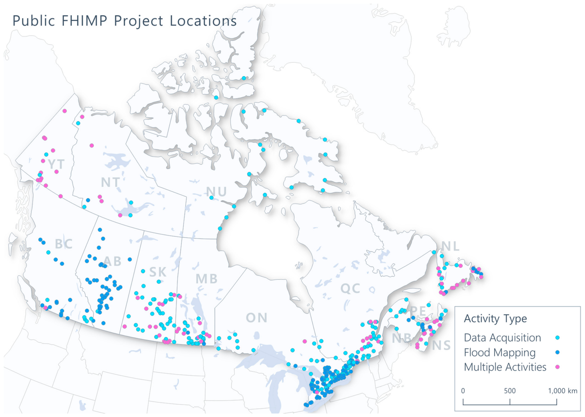
Figure 1. FHIMP project locations across Canada (image source: [17]).
Water 18 01592 g001
Figure 2. Schematic view of cross-section survey.
Water 18 01592 g002
Figure 3. Lacombe flood study area; road and hydrography layers obtained from [29].
Water 18 01592 g003
Figure 4. Kinuso flood study area; road and watershed layers obtained from [31], imagery is from [32], National Hydro Network (NHN) layer is from [33].
Water 18 01592 g004
Figure 5. Wolf Creek (a) and typical tributary (b) conditions noted during the Lacombe site visit (13 June 2023).
Water 18 01592 g005
Figure 6. Swan River conditions during the Kinuso survey (10 September 2024).
Water 18 01592 g006
Figure 7. Typical plan view and cross-section profile of the Swan River.
Water 18 01592 g007
Figure 8. Histogram of survey and DTM differences for different classes of survey data at Kinuso.
Water 18 01592 g008
Figure 9. Instantaneous annual peak flows versus annual maximum daily flows for West Whitemud Creek near Ireton.
Water 18 01592 g009
Figure 10. Bulletin 17C (EMA) flood frequency analysis results for West Whitemud Creek near Ireton.
Water 18 01592 g010
Figure 11. The 1996 daily flow hydrograph for Swan River near Kinuso.
Water 18 01592 g011
Figure 12. Yearly maximum 5-day moving average flow for Swan River near Kinuso.
Water 18 01592 g012
Figure 13. Scaled hourly hydrographs for Swan River near Kinuso.
Water 18 01592 g013
Figure 14. Coarsely adjusted hydrographs with peak flow spikes based on Bulletin 17C (EMA) flood frequency analysis results for Swan River near Kinuso.
Water 18 01592 g014
Figure 15. Smoothed hydrographs for Swan River near Kinuso.
Water 18 01592 g015
Figure 16. Final Method 1 hydrographs for Swan River near Kinuso.
Water 18 01592 g016
Figure 17. Balanced hydrographs with peak flow spikes for Swan River near Kinuso.
Water 18 01592 g017
Figure 18. Final Method 2 hydrographs with smoothed peaks for Swan River near Kinuso.
Water 18 01592 g018
Figure 19. Example of coupled 1D/2D model domain in the Lacombe flood study. Note: LOB = left overbank and ROB = right overbank.
Water 18 01592 g019
Figure 20. Comparison of the LiDAR-derived DTM (left) and the composite DTM with mosaicked interpolated channel bathymetry (right).
Water 18 01592 g020
Figure 21. Example of 2D model domain in the Kinuso flood study.
Water 18 01592 g021
Figure 22. Swan River changes between 2023 (top) and 2024 (bottom).
Water 18 01592 g022
Figure 23. Low-flow calibration results (14 September 2024 flows).
Water 18 01592 g023
Figure 24. Comparison of simulated and observed water levels (surveyed 2024 flood HWMs).
Water 18 01592 g024
Figure 25. Comparison of simulated 1:1000-year flood under quasi-steady-state and unsteady-state conditions.
Water 18 01592 g025
Table 1. WSC stations used for regional flood frequency analysis.
WSC StationPeriod of RecordYears of Record 1Gross Drainage Area (km2)Effective Drainage Area (km2)
West Whitemud Creek near Ireton (05DF007)1976–2021416553
Block Creek near Leedale (05CC010)1976–2020355757
Maskwa Creek No. 1 above Bearhills Lake (05FA014)1972–2021337961
Haynes Creek near Haynes (05CD006)1978–202136165165
Bigknife Creek near Gadsby (05FC002)1967–202142281194
Lloyd Creek near Bluffton (05CC009)1965–202035239239
Waskasoo Creek at Red Deer (05CC011)1984–202032487250
Whitemud Creek near Ellerslie (05DF006)1969–202042330301
Note: 1 Excluding years with missing data in the period of record.
Table 2. Parameters of the final multilinear regression analysis.
Flood
Frequency
Scenario
Multilinear Regression ParametersAdjusted
R2
ab
X1 = Effective Drainage Area
c
X2 = Basin Slope
1:20.00641.2620.3390.602
1:50.00721.3580.5440.727
1:100.00801.4040.6470.783
1:200.00911.4370.7270.819
1:350.00981.4640.7870.843
1:500.01021.4800.8240.854
1:750.01091.4960.8620.866
1:1000.01141.5050.8870.871
1:2000.01231.5320.9480.885
1:3500.01291.5530.9950.891
1:5000.01341.5671.0250.895
1:7500.01391.5831.0600.898
1:10000.01421.5921.0800.899
Table 3. Lacombe flood study model details.
ParameterValue
Full 2D Reach Length (km)18
Coupled 1D/2D Reach Length (km)12
Computational SolverSWE-ELM
Time Step (seconds)1
Approximate Simulation Time (hours)10
Number of Cells in 2D Domain94,342
Smallest/Largest Cell Size (m)2/20
Number of Surveyed Cross-Sections 129
Number of Interpolated Cross-Sections65
Cross-Section Interpolation Distance (m)100
Number of Lateral Structures31
Number of Breaklines269
Number of 2D Connections91
Table 4. Kinuso flood study model details.
ParameterValue
Fully 2D Reach Length (km)24
Computational SolverSWE-ELM
Time Step (seconds)4/2
Approximate Simulation Time (hours)4
Number of Cells128,740
Smallest/Largest Cell Size (m)3/30
Number of Breaklines143
Number of 2D Connections77
Table 5. Summary of high-flow calibration results.
Event YearPeak Flow (m3/s)Average Water Level Difference (Simulated Minus Observed) (m)Root Mean Square Error (m)
1979362−1.521.54
1982200−1.471.47
1983571−0.100.48
1986332−0.200.86
1988654−0.590.60
2011582−0.240.24
20186370.000.07
20244770.050.21
Disclaimer/Publisher’s Note: The statements, opinions and data contained in all publications are solely those of the individual author(s) and contributor(s) and not of MDPI and/or the editor(s). MDPI and/or the editor(s) disclaim responsibility for any injury to people or property resulting from any ideas, methods, instructions or products referred to in the content.