On the Mean Excess Plot Measures of Chilean Glacier Mass Balance Data

Abstract

We study the extreme behavior of six central Chile glacier mass balance series facing significant retreats and ice wastage due to climate variability and change. This has led to reduced meltwater availability in dry seasons, increasing competition for downstream water resources. Understanding glacier mass balances is crucial for predicting future water availability in scenarios with higher water demands. We used Extreme Value Theory tools to analyze the data and identify extreme events. The main objective of this study is to statistically analyze glacier mass losses in Chile, using mass balance data collected from both national and international sources. The results show high heterogeneity in the extreme behavior of glaciers, with some showing an approximately exponential tail (Guanaco Glacier), others exhibiting stability with slight tails (Echaurren Norte and Mocho Glaciers) and one (Amarillo Glacier) with a highly unstable structure. The other analyzed glaciers (Juncal Norte and Juncal Sur) have slight and potentially limited tails. These results confirm the high importance of studying glaciers in the Andes in order to better understand their responses to climate change, an important and relevant aspect for the future management of glacier melt water resources.

1. Introduction

The loss of freshwater, a strategic resource for life in Chile, generates significant impacts due to the projected consequences on natural and human systems. For example, the study of glaciers identifies geographical and geomorphological effects associated with changes in the dynamics of lakes, lagoons, and rivers, as well as environmental impacts that affect the biodiversity of flora and fauna and the surrounding human communities. In the current context of climate change, the rise in sea level, directly linked to the retreat and shrinking of glaciers, creates a particularly worrying scenario for the country.

Chile has approximately 24,000 km² of surface area covered by glaciers, distributed across some 26,000 glacial units, according to the latest glacier inventory. This represents roughly 76% of the glacial surface area of South America. This distribution is heterogeneous, concentrated mainly in the Aysén and Magallanes regions, where more than 50% of the total glaciers are located. These ice bodies are a crucial source of water, especially in arid zones, so their retreat poses challenges for water security, ecosystems, and land-use planning. This inventory also reflects the following: in the last decade, a phenomenon of glacial fragmentation has been observed; that is, while some glaciers have decreased in surface area, there has been an increase in the total number of glaciers, reflecting complex processes of division and retreat.

Despite the monitoring work carried out by national and international institutions, such as the Chilean General Directorate of Water (DGA) or the World Glacier Monitoring Service (WGMS), significant challenges remain in understanding glacial dynamics and characterizing their temporal and spatial variability. For example, the Juncal Sur Glacier, located in the Valparaíso Region, lost approximately $25\%$ of its surface area between 1955 and 2018 (see [1]), which highlights the urgent need for rigorous statistical tools that strengthen quantitative interpretation and support the development of adaptation strategies to climate change. Previous studies on Chilean glaciers have largely relied on linear trends, which often fail to account for the rapid acceleration of ice loss during extreme events, such as the ongoing “megadrought” (2010–present) and severe warm anomalies. Extreme Value Theory (EVT) is needed beyond standard trend analysis to specifically model these non-linear, high-impact events and to address significant gaps in long-term observational data. An important factor here is also data availability. The dynamical system justification for using mean excess plot approaches is given, for example, in [2]. Previous studies failed to address the impact of extreme events, unprecedented drought conditions, data scarcity, spatial variability, debris cover, glacier dynamics, and related geographical issues.

The geodetic reconstructions presented indicate mass loss since at least 1955, with recent acceleration. The ice core extracted in 2008 shows that the glacier has a cold base, with a temperature inversion in the first 60 m attributed to atmospheric warming. The analysis revealed seasonal cycles of accumulation, significant melting during the summer, and limited sublimation. Furthermore, positive correlations were identified between the Guanaco Glacier’s mass balance and the ENSO index, as well as with the position of the South Pacific Subtropical High (SPSH).

The local study of the Pascua-Lama region (Chilean Andes, 29° S and 5000 m a.s.l.), documented by [3], details a monitoring program initiated in 2003, which allowed for the analysis of several glaciers in an arid, subtropical, and high-altitude environment. Glaciological measurements indicated variability in surface mass balance, influenced primarily by winter accumulation. A multi-temporal analysis revealed a 29% reduction in glacial surface area between 1955 and 2007, with an acceleration toward the end of the 20th century. The observed variations are closely related to local and regional climatic parameters, highlighting the sensitivity of these glaciers to climate change and their importance for water availability in arid zones.

In another local study from a different region, in this case Alaska, the findings are captured in the article by [4], where GRACE satellite observations were used to assess glacial mass loss in Alaska between 2002 and 2014. A three-parameter model was developed based on snow and temperature data from the ERA-Interim reanalysis, fitted to the GRACE series. This model explained 94% of the observed variability and was used in conjunction with Community Earth System Model simulations to project losses up to 2100. A mass loss of between −80 and −110 Gt/year is estimated, contributing to a sea level rise of $19\pm 4$ mm during the 21st century.

Regarding projections, studies such as [5] show that projections made using global climate models (GCMs) indicate a significant loss of glacial water input in the Andes, with considerable variations between basins, where the highest amount of water will be reached before mid-century. This highlights the urgent need to develop water adaptation strategies differentiated by region and basin, considering the projected changes in glacial contribution and its impact on socio-ecological systems, especially during dry seasons or drought years.

This approach to projections has also evolved methodologically; thus, in Ref. [6], it is noted that for future projections of glaciers, the focus shifts to three indicators: glacier area, ice volume, and mass balance. This change highlights the need for a more macroscopic assessment of the impacts of climate change on glaciers and regional water resources. Unlike the detailed, micro-level analysis of historical data, future projections emphasize the potential impact of glacial retreat on water supply.

This literature review shows that the study of glaciers in Chile has advanced significantly, especially in the last 10 years. Most of the studies presented agree on a sustained loss of glacial mass and surface area, with direct implications for the amount of water in sensitive regions. This decrease is closely related to rising temperatures, although the influence of non-climatic factors on local behavior is also acknowledged.

In this study, we applied mean excess plots to statistically analyze the mass balance of glaciers in Chile using data collected from national and international public sources, such as the WGMS and selected national studies. We identified spatial and temporal patterns, estimated trends, and developed methodology to improve the interpretation and modeling of this data. In particular, we analyzed the short-term mass balance of Chilean glaciers through data analysis and visualization, comparing mass loss patterns in different regions. We used the software tools R 4.1.1 [7] and Python 3.12.13.

2. Materials and Methods

2.1. State of the Art

Glacial behavior in Chile, especially in the Andes, has been extensively studied in recent decades due to the factors already described in this work, particularly in the case of the Echaurren Norte Glacier, which is the representative or indicator glacier of the health and evolution of glaciers in this part of the Andean mountain range. It was selected by the DGA (General Directorate of Water) in 1975 to initiate a measurement program whose main objective was to monitor the mass balance. These various investigations have shown that changes in glacier mass are mainly related to temperature changes; even so, there are non-climatic factors that influence their behavior. Within [8], it is explained that there are glacier behaviors that are attributed to non-climatic factors; it is confirmed that glacial activity depends on non-climatic factors, and that most glacial variations originate from the temperature increases observed in recent years. This has a considerable impact on glacial fluctuations. It also indicates that $5.6\%$ of the total glaciers currently recorded in the country are affected. Of these, only $6\%$ have shown a net increase in the analyzed periods.

Regarding large-scale patterns, the study [9] describes the sustained decrease in snow cover in the Andes, which has been 19% per decade between 2001 and 2022. This phenomenon has significantly affected the flows of rivers such as the Aconcagua and the Maipo, with reductions of 60% and 40% since the 1980s, respectively. These losses are associated with changes in wind patterns influenced by the Antarctic Oscillation and climate change. The scarcity of snow has intensified water stress in rural and indigenous communities, leading to migration and depopulation.

Even so, the scarcity of detailed and distributed models for Chilean glaciers has been identified as a critical limitation by [10], which indicates that Chilean glaciers are decreasing in size and mass, although the available information does not yet allow for a comprehensive view of past and future changes. While local and remote sensing studies exist, the lack of distributed and physically detailed models is evident. The study highlights the “glaciological regions of Chile” as key to future research, as well as the limitations in mass balance data and in the representation of spatial processes. Factors influencing glacier modeling include: the ablation model, temperature extrapolation, snow redistribution, and climate scenarios. Similarly, Ref. [11] analyzes the evolution of the mass balance of the Guanaco Glacier, located in the arid Chilean Andes at over 5000 m above sea level. The study covers three periods (recent: 2002–2015; historical: 1955–2005; and past: prior to 1900) and uses glaciological, geodetic, and ice core data. It demonstrates that since 2002, the mass balance has been predominantly negative. The study determined that the glacier is particularly sensitive to precipitation in an environment characterized by low temperatures, high radiation, strong winds, and loss through sublimation.

Regarding methodologies, there has been an evolution from traditional techniques to more robust and adaptive approaches. Statistical tools such as the t-Hill estimator allow for a better characterization of the extreme behavior of glaciological series with greater precision. Meanwhile, the use of distributed physical models, satellite observations, and more recent machine learning techniques expands the possibilities for estimating and projecting the mass balance in both monitored and unmonitored glaciers.

Furthermore, future projections demand a shift in the scale of analysis, moving from detailed, focused assessments to integrative methodologies that utilize indicators such as ice volume and glacier extent. This transition addresses the need to understand the impact of glacial retreat not only on the hydrological cycle or system, but also on ecosystems, local communities, and other relevant factors.

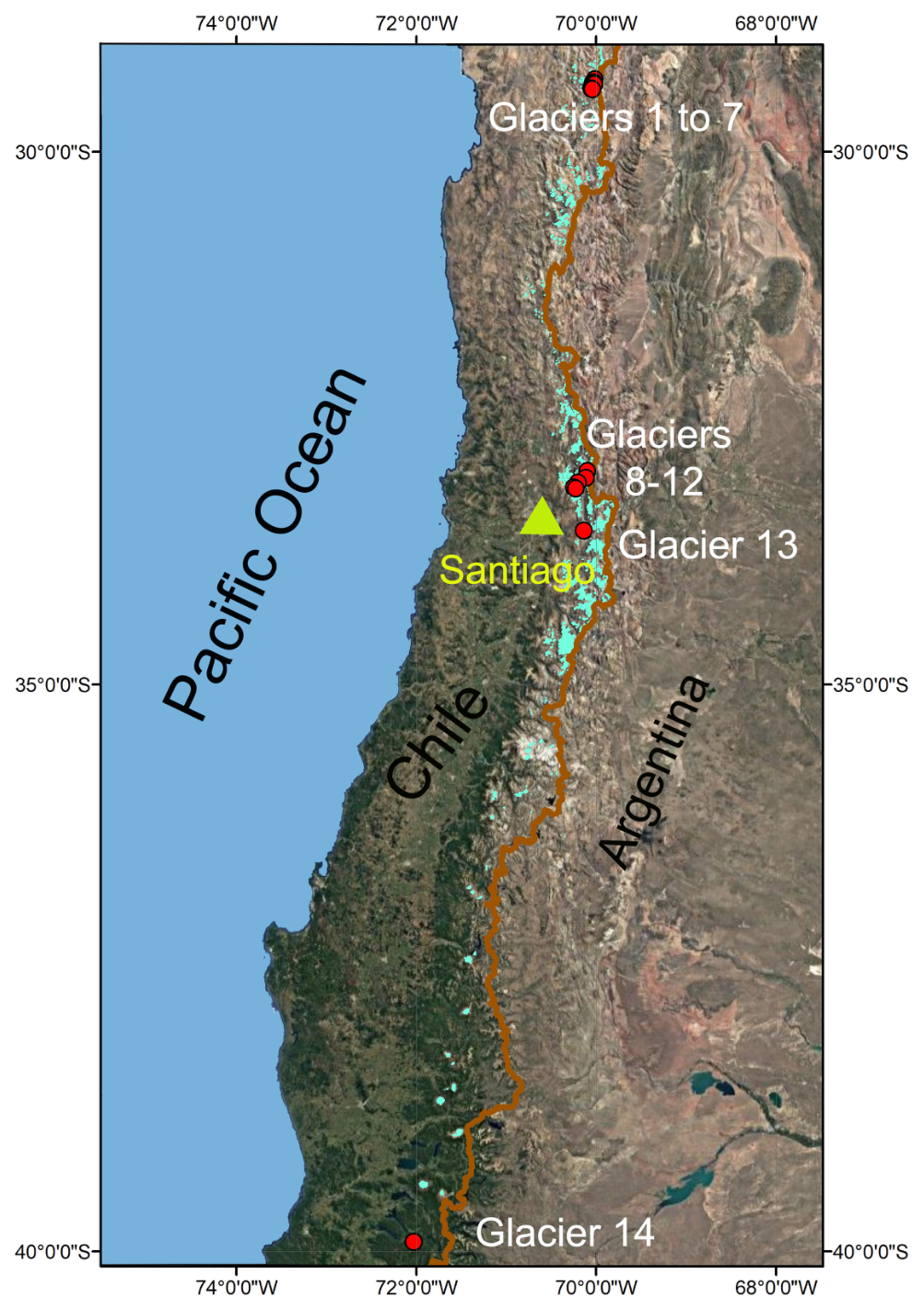
In conclusion, several challenges were identified, including the scarcity of local data, the limited spatial resolution of some models, and the need for calibration in specific watersheds. This underscores the importance of strengthening glaciological research in Chile through the combined use of data, modeling, and advanced technologies, which is the aim of this research. The following Figure 1 shows the area map, giving a clear spatial framework for the analyzed glaciers.

Table 1. Basic characteristics of the studied glaciers.

Number	Name	Lat (°)	Long (°)	Mean Alt. (m)	Alt. Range (m)	Method
1	Estrecho	$-29.2969$	$-70.01437$	5267	5506–5067	Direct (glaciological)
2	Esperanza	$-29.3297$	$-70.0369$	5081	5146–5027	Direct (glaciological)
3	Toro 1	$-29.3300$	$-70.0190$	5222	5241–5176	Direct (glaciological)
4	Toro 2	$-29.3326$	$-70.0276$	5085	5110–5058	Direct (glaciological)
5	Guanaco	$-29.3490$	$-70.0190$	5171	5360–5011	Direct (glaciological)
6	Ortigas 1	$-29.3875$	$-70.0540$	5057	5233–4812	Direct (glaciological)
7	Ortigas 2	$-29.3940$	$-70.0425$	5101	5155–5013	Direct (glaciological)
8	Juncal Norte	$-33.0296$	$-70.0984$	4556	5865–2903	Indirect (geodetic)
9	Juncal Sur	$-33.0935$	$-70.1163$	4391	5760–3776	Indirect (geodetic)
10	Olivares Beta	$-33.1380$	$-70.2020$	4509	4896–3863	Direct (glaciological)
11	Paloma Norte	$-33.1797$	$-70.2497$	4624	4868–4463	Direct (glaciological)
12	Olivares Alfa	$-33.1938$	$-70.2252$	4563	5019–4272	Direct (glaciological)
13	Echaurren Norte	$-33.5820$	$-70.1363$	3794	4038–3673	Direct (glaciological)
14	Mocho	$-39.9200$	$-72.0300$	1964	2399–1407	Direct (glaciological)

illustrates the studied glaciers and their basic characteristics.

2.2. Prior Methodological Background

The glacial mass balance is determined by the difference between snow accumulation in winter and snow ablation during summer, including melting and sublimation. This seasonal cycle is fundamental for assessing the health and evolution of glaciers, reflecting the climatic effects on these ice masses [12]. The WGMS has been collecting and publishing this data since 1894 in an effort to improve the understanding of glaciers worldwide and thus have the tools to protect this resource. In the national context, the relevance of the mass balance increases due to the climatic diversity of the Andes Mountains, which ranges from arid zones in the north, through semi-arid regions in the center, to humid ice fields in Patagonia (see [10]). Recent studies in the central macrozone, an area encompassing the Valparaíso, Metropolitan, O’Higgins, and Maule regions, show a marked retreat in glaciers such as Juncal Sur, which lost approximately $21\%$ of its surface area between 1955 and 2013/14 (see [13]), and Olivares Beta lost 34% of its area between 1955 and 2018 (Rivera, 2019 [1]).

In this area, the Glaciology Laboratory, founded by Professor Andrés Rivera in 1997, is a key source of data.

Given the accelerated retreat, it is essential to implement rigorous statistical analyses to understand the variability and trends in mass balance.

2.3. Adopted Estimators

The methodologies proposed by [2] allow modeling the inherent uncertainty, and the appropriate design of sampling plans minimizes errors, improving the accuracy of parametric, non-parametric, and semi-parametric models. In [14], the t-Hill estimator for heavy tails is introduced, along with its adjusted version, the t-lgHill estimator [15]. The Zipf estimator, based on the one proposed by Kratz and Resnick (1996) [16], as cited in [15], relies on a least-squares regression between the theoretical quantiles of a Pareto distribution and the logarithms of the order statistics.

We denote by $X_1,X_2,\dots ,X_n$ independent identically distributed (i.i.d.) random variables (r.v.s) with cumulative distribution function (c.d.f.) F such that $\overline{F}\in R{V}_{-\alpha }$ with $\alpha >0$. This means that there exists a positive limit:

$$\underset{t\to \infty }{\lim }{\displaystyle \frac{\overline{F}\left(tx\right)}{\overline{F}\left(t\right)}}=x^{-\alpha }$$

for $x>0$ with some $\alpha >0$. The number $-\alpha$ is called the index of regular variation. Denote the corresponding increasing order statistics by

$$X_{1,n}\le X_{2,n}\le ...\le X_{n,n}$$

Under the assumption that the extreme data follow a Pareto-like distribution, the relationship is expected to be

$$\left(-\log \left(1-{\displaystyle \frac{i}{n+1}}\right),\log X_{i,n}\right),1\le i\le n$$

(1)

which is approximately linear, with slope equal to $\gamma :=1/\alpha$. From this relationship, the Zipf estimator for a number $k_n$ of extreme observations is defined as

$${\widehat{\gamma }}_{\mathrm{zipf}}\left(k_n\right)=\mathrm{slope}\mathrm{of}\mathrm{the}\mathrm{regression}\mathrm{of}\left(-\log \left(1-{\displaystyle \frac{i}{k_n+1}}\right),\log X_{n-k_n+i,n}\right),1\le i\le k_n$$

(2)

Subsequently, the scale parameter $\sigma$ was estimated using

$$\widehat{\sigma }=X_{n-k_n+1,n}·\widehat{\gamma }$$

(3)

We use the following notations in the article: For the Hill estimator, this is expressed as

$${\mathrm{DE}}_{\mathrm{Hill}}=H_{k_n,n}·\sqrt{k_n}$$

(4)

For the Zipf estimator,

$${\mathrm{DE}}_{\mathrm{Zipf}}={\widehat{\gamma }}_{\mathrm{zipf}}\left(k_n\right)·\sqrt{{\displaystyle \frac{k_n}{2}}}$$

(5)

And for the t-Hill estimator, we use

$${\mathrm{DE}}_{\mathrm{t-Hill}}=H_{k_n,n}^{*}·\sqrt{k_n}\left({\displaystyle \frac{1+H_{k_n,n}^{*}}{1+2H_{k_n,n}^{*}}}\right)$$

(6)

Manipulating $k_n$ can improve stability and reduce bias in estimates. The Zipf estimator may show visual stability but has significant bias in small samples. The t-Hill estimator is more robust and reliable in such cases.

In this manuscript, we use only the Mean Excess Function (MEF) and POT approach from EVT. In particular, we used the coefficient of variation (CV) as a justification to determine where the tail begins (see [17]). This is a widely studied topic in the literature, with various methods available for this purpose, but from a practical point of view, we decided on CV. We do not need stationarity and weak dependence to apply our methods since we are not using any asymptotic approximation; rather, we rely on theoretical justifications obtained in [18]. Ref. [18] achieves EVT flexibilization by introducing a generalized Hill estimator, using a mean of order to improve heavy-tailed data modeling. This approach provides more accurate, adaptable estimates for small, heavy-tailed samples, validated by asymptotic normality and practical, alternative Hill plots outside of 2nd-order frameworks. During the original research, we checked the seasonality (mostly visually) and autocorrelations.

2.3.1. Fundamentals of Extreme Value Theory

Extreme events, such as floods, wildfires, mass bankruptcies, or financial crises, pose significant risks to society. Due to their infrequent nature, modeling them statistically is challenging, as empirical data is scarce (see [17]). In this context, Extreme Value Theory (EVT) is proposed as a solution. It provides tools for modeling the behavior of rare events, allowing extrapolation beyond the observed range of the data. The Extreme Types Theorem has been provided by Gnedenko, 1943 [19].

2.3.2. Peaks over Threshold (POT) Method

An alternative to the block maxima approach is the Peaks Over Threshold (POT) method, which was used in this study. This method considers data excesses above a high threshold, t. Under this approach, if $F\in D\left(G_{\gamma }\right)$, then the conditional distribution of excesses $X_t=X-t|X>t,$ is approximated by a generalized Pareto (GP) distribution:

$$H_{\gamma }\left(x\right)=1-{\left(1+{\displaystyle \frac{\gamma x}{\psi }}\right)}^{-1/\gamma },x>0,$$

(7)

where $\psi >0$ is the scale parameter and $\gamma$ is the shape parameter.

2.4. Threshold Selection: Mean Excess Function

The appropriate selection of the threshold t is emphasized, as it is critical to ensuring a good fit of the GP model. One strategy implemented within the text is the use of the Mean Excess Function (MEF):

$$e\left(t\right)=\mathbb{E}[X-t\mid X>t]={\displaystyle \frac{\psi +\gamma t}{1-\gamma }},\gamma <1.$$

(8)

Its empirical version is defined as

$$\widehat{e}\left(t\right)={\displaystyle \frac{1}{N_t}}{\displaystyle \sum _{i=1}^n}(x_i-t)·{\mathbf{1}}_{\{x_i>t\}},$$

(9)

where $N_t$ is the number of observations that exceed the threshold t. An approximately linear relationship in the graph $t\mapsto \widehat{e}\left(t\right)$ suggests that the excesses from this threshold follow a GP distribution.

The influence of temporality is also important, as evaluated in extreme-temperature studies [20,21], where it is recommended to eliminate non-parametric trends in mean and standard deviation to consider the extremes as stationary, facilitating extrapolation and calculation of representative return levels.

The graphs of the empirical mean excess values $e_{k,n}$, introduced in (9), can be constructed in two alternative ways: by plotting $e_{k,n}$ against k, or $e_{k,n}$ against $x_{n-k,n}$. Recalling the discussion in the previous subsection, the aim is to analyze the behavior of the plotted values of $e_{k,n}$ as k decreases, or equivalently, as the values $x_{n-k,n}$ increase. Depending on the slope of the MEF, three main cases are distinguished [22]:

• Positive slope ($\mathbf{0}\mathbf{<}\mathsf{\gamma }\mathbf{<}\mathbf{1}$): The distribution has a heavy tail with a finite mean. In this scenario, the MEF grows linearly for high thresholds, allowing it to be approximated by a Generalized Pareto Distribution (GPD). This linearity facilitates the estimation of the shape parameter $\gamma$ and confirms that the tail is heavy but has a finite mean.
• Negative slope ($\mathsf{\gamma }\mathbf{<}\mathbf{0}$): The distribution has a short tail with a finite upper bound $x_F$. The MEF decreases towards zero as the threshold approaches $x_F$, reflecting that there are no values above this maximum. This case corresponds to the domain of attraction of the Weibull distribution.
• Zero slope ($\mathsf{\gamma }\mathbf{=}\mathbf{0}$): The distribution is similar to an exponential. The MEF remains practically constant for all thresholds, a typical characteristic of the Gumbel distribution class. This behavior indicates a light tail with no finite upper bound.

In practical terms, the shape of the ME plot allows us to infer the nature of the tail: a linearly increasing ME plot suggests a heavy tail ($\gamma >0$), a decreasing ME plot indicates a short tail ($\gamma <0$), and a constant ME plot corresponds to an exponential tail ($\gamma =0$) [22]. Furthermore, the theoretical results of Ghosh and Resnick formalize how to scale the points of the ME plot so that they converge to the theoretical line or the limit set depending on the value of $\gamma$, ensuring a robust interpretation in the analysis of extreme values. This can be visualized as shown in [23].

2.5. Alternative: Coefficient of Variation

Ref. [24] proposes a more robust approach based on the coefficient of variation (CV) of excesses:

$$CV\left(X_t\right)={\displaystyle \frac{\sqrt{\mathrm{Var}\left(X_t\right)}}{\mathbb{E}\left(X_t\right)}}={\displaystyle \frac{1}{\sqrt{1-2\gamma }}},\gamma <{\displaystyle \frac{1}{2}}.$$

(10)

This value is constant for a GP with a valid tail and depends only on $\gamma$. The empirical version is

$$\widehat{cv}\left(t\right)={\displaystyle \frac{\mathrm{sd}\{x_j-t\mid x_j>t\}}{\mathrm{mean}\{x_j-t\mid x_j>t\}}}.$$

(11)

A plot of $t\mapsto \widehat{cv}\left(t\right)$ is expected to be approximately constant if the data above t fit a GP well.

Transformation for Heavy Tails

Ref. [17] also adopted the methodology of [24]. This is because the variance of $CV\left(X_t\right)$ only exists if $\gamma <1/4$; the following transformation is proposed:

$$Y={\displaystyle \frac{\sigma X}{X+\sigma }},\mathrm{con}\sigma ={\displaystyle \frac{\psi }{\gamma }},$$

(12)

which converts $X\sim GP(\psi ,\gamma )$ into $Y\sim GP(\psi ,-\gamma )$, allowing the methodology to be applied even when $\gamma$ is large. This can be especially important due to the distribution of the data.

2.6. Automatic Threshold Selection Using Multiple Contrast

The procedure proposed by Castillo and Padilla (2016) [24] used in [17] is based on testing the null hypothesis of CV constancy over a set of thresholds. Let $q_k$ be the empirical quantile corresponding to the level $p_k$; the statistic is defined as follows:

$$T_m=n{\displaystyle \sum _{k=0}^m}{p}_k{\left(CV\left(q_k\right)-c_{\gamma }\right)}^2,$$

(13)

where $c_{\gamma }$ is the value that minimizes $T_m$. From this, an estimate of the tail index is obtained:

$$\widehat{\gamma }={\displaystyle \frac{1-c_{\gamma }^{-2}}{2}}.$$

(14)

The procedure is repeated by eliminating the first thresholds until the constancy hypothesis is accepted, indicating that excesses above the current threshold can be adequately modeled by a GP.

2.7. Hill Estimator (and t-Hill)

We define the Hill estimator [25] of the extreme index $\gamma$ by

$$H_{k,n}={\displaystyle \frac{1}{k}}{\displaystyle \sum _{i=1}^k}\log \left({\displaystyle \frac{X_{n-i+1,n}}{X_{n-k,n}}}\right).$$

(15)

The t-Hill technique was developed by [14] as a natural robustification of the Hill estimator (15), and further studied by [15]. It is given by (16)

$${\widehat{\gamma }}_k={\displaystyle \frac{1}{{\widehat{\alpha }}_k}}=H_{k,n}^{*}={\left({\displaystyle \frac{1}{k}}{\displaystyle \sum _{i=1}^k}{\displaystyle \frac{X_{n-k,n}}{X_{n-i+1,n}}}\right)}^{-1}-1$$

(16)

This methodology was also successfully applied in the context of Extreme Value Theory (EVT) to glaciers in the work of [15].

2.8. Data Types

It should be clarified that the data, or the way in which they are communicated, correspond to in situ observations of snow and ice, which allow the quantification of the mass balance using the metric m w.eq./year, that is, meters of water equivalent per year or in terms of the thickness of a water sheet equivalent to the volume of mass gained or lost. This is the case for the data from Juncal Norte and Juncal Sur, reported by [9], and all glacier mass balance data in general. An integrated database was created from national and international sources to analyze glacier data from 2000 onwards. The statistical tools R and Python were used to explore trends and patterns in glacial mass balance behavior.

2.9. Direct Data Definition

The data used in this study come from the WGMS2025 database [26] and public reports from the General Directorate of Water Resources (DGA) corresponding to the Juncal Norte Glacier [27]. These sources provide systematic and validated information on the temporal evolution of the glacial mass balance, allowing for consistent analysis across different climatic and geographic contexts in Chile.

This type of data is measured using the unit m w.e. (meters of water equivalent), which corresponds to a standardized way of expressing the mass balance of glaciers, as previously mentioned.

2.10. Indirect Data Definition

Historical mass balance data for the Juncal Norte and Juncal Sur Glaciers, obtained from the study by [9], are considered. These data provide a solid basis for analyzing the temporal variability and extreme behavior of these glaciers in central Chile. These records allow for the evaluation of trends, anomalies, and structural changes in glacial dynamics under different climatic scenarios.

In parallel, a systematic review of environmental assessment reports and technical documents prepared by public and private institutions was developed, with the purpose of contextualizing the quantitative results within the framework of territorial planning, environmental management and current public policies, thus establishing a link between statistical evidence, decision-making and the sustainable management of water resources.

2.11. Statistical Analysis

Regarding the statistical analysis, techniques such as time series analysis and extreme value modeling were applied using the various techniques already reviewed.

• Data Loading from Official Sources: Datasets from the World Glacier Monitoring Service (WGMS) are imported, in addition to supplementary databases.
• Database integration: Mass balance records are linked to geomorphological information of glaciers by a join using the unique identifier glacier_id, allowing each observation to be correctly associated with its respective glacier.
• Spatial filtering: Glaciers located exclusively within Chilean territory are selected using this criterion, in order to restrict the study to the geographic area of interest.
• Data cleaning: The annual mass balance series undergoes a cleaning process that includes:
  • Removal of infinite values.
  • Removal of missing values.
  • Elimination of duplicate records.
• Glacier Quality Control: The total number of records per glacier is counted, and, in parallel, the number of valid annual mass balance observations. This procedure allows for the evaluation of the temporal density of the data and the selection of glaciers with sufficiently informative series.
• Temporal standardization: The available years are ordered in ascending order, allowing for their correct interpretation in time series analysis.
• Construction of individual time series: For each selected glacier, its respective annual mass balance time series is constructed, considering the common period already given from the year 2000, according to the systematic availability of data.
• Exploratory Analysis: Histograms, time-series graphs, and descriptive mass balance measures are generated, allowing the identification of variability patterns, asymmetries, trends, and possible anomalies.
• Preparation for Extreme Value Theory (EVT): The tails of interest are selected from the mass balance (mainly negative extremes), transforming the data as appropriate to ensure positivity and numerical stability.

2.12. Modeling Extreme Values

To reduce the influence of outliers and improve the reliability of the results, tailings analysis techniques are incorporated. That is, for modeling extreme values, the aforementioned “peaks threshold” methodology is followed. Making an appropriate selection of the threshold t is critical to ensuring a good fit of the GP model. A common strategy is the use of the Mean Excess Function (MEF):

$$e\left(t\right)=\mathbb{E}[X-t\mid X>t]={\displaystyle \frac{\psi +\gamma t}{1-\gamma }},\gamma <1.$$

(17)

where $N_t$ is the number of observations exceeding the threshold t. An approximately linear relationship in the graph $t\mapsto \widehat{e}\left(t\right)$ suggests that the excesses beyond this threshold follow a GP distribution.

This assessment is initially performed by visually inspecting the Mean Excess Function (MEF) graph, using the 0.50th percentile, corresponding to the median, as the initial threshold. This threshold is selected because it allows for a suitable balance between statistical stability and a sufficient number of exceedances, thus facilitating the identification of stable regions where the slope of the graph remains approximately constant.

2.13. Coefficients of Variation

The procedure proposed by Castillo and Padilla [24] is used (as indicated in [17]; it is based on testing the null hypothesis of the constant coefficient of variation over a set of thresholds).

To test whether the data really follow a GPD, we have to look at how $cv\left(t\right)$ behaves for different $t.$ Therefore, let $q_k$ be the empirical quantile corresponding to the level $p_k$; the statistic is defined as follows:

$$T_m=n{\displaystyle \sum _{k=0}^m}{p}_k{\left(CV\left(q_k\right)-c_{\gamma }\right)}^2,$$

(18)

where $c_{\gamma }$ is the value that minimizes $T_m$. From this, an estimate of the tail index is obtained:

$$\widehat{\gamma }={\displaystyle \frac{1-c_{\gamma }^{-2}}{2}}.$$

(19)

The procedure is repeated, eliminating the initial thresholds, until the constancy hypothesis is accepted, indicating that excesses above the current threshold can be adequately modeled using a GP. For comparative purposes and to validate the robustness of the analysis, this procedure is applied considering two initial threshold ranges. The first corresponds to the quantile range between 0.50 and 0.95, which is adopted as the main tentative threshold for this work. The second range considered corresponds to the quantiles between 0.95 and 0.99, representing a more extreme and restrictive threshold, designed to capture only the most severe events. Comparing both ranges allows for evaluating the sensitivity of the results to the chosen threshold and strengthens the interpretation of the extreme dynamics of the glacial mass balance.

The procedure is evaluated both analytically, using the value of the statistic $T_m$, and graphically, using the visual version of the constancy test for the coefficient of variation. In this representation, the stability of $CV\left(t\right)$ as a function of the threshold constitutes a direct visual indicator of the suitability of the GPD model to describe the tail of the distribution.

2.14. Application of the Hill, t-Hill, and Zipf Methodologies

To analyze the left tail of the glacier’s annual mass balance, the Hill, t-Hill, and Zipf estimators were applied.

• Data Preparation

Emphasis is placed on the selection of glacier data and the transformation of negative balances to positive ones in order to apply extreme estimators. Formally, if $X_i$ represents the annual mass balance, the inverted left tail is defined as

$$X_i^{+}=-X_i,\mathrm{para}{X}_i<0.$$

The values are ordered from lowest to highest:

$$X_{\left(1\right)}^{+}\le X_{\left(2\right)}^{+}\le \cdots \le X_{\left(n\right)}^{+}.$$

2.

Hill Estimator

Let $X_{1,n}\le \cdots \le X_{n,n}$ be the ordered sample. For $k=1,\dots ,n-1$, the Hill estimator is defined as

$${\widehat{\gamma }}_{k,n}={\displaystyle \frac{1}{k_n}}{\displaystyle \sum _{i=1}^{k_n}}\log \left({\displaystyle \frac{X_{n-i+1,n}}{X_{n-k_n,n}}}\right).k=1,\dots ,n-1.$$

The asymptotic standard deviation used is

$$\mathrm{SD}\left({\widehat{\gamma }}_{k,n}\right)={\displaystyle \frac{{\widehat{\gamma }}_{k,n}}{\sqrt{k_n}}}.$$

3.

t-Hill estimator

The implemented t-Hill estimator is defined as

$$H_{k,n}^{*}={\left({\displaystyle \frac{1}{k_n}}{\displaystyle \sum _{i=1}^k}{\displaystyle \frac{X_{n-k,n}}{X_{n-i+1,n}}}\right)}^{-1}-1,k=1,\dots ,n-1,$$

The asymptotic standard deviation used is

$$\mathrm{SD}\left({\widehat{\gamma }}_{k,n}^t\right)={\displaystyle \frac{{\widehat{\gamma }}_{k,n}^t}{\sqrt{k_n}}}\left({\displaystyle \frac{1+{\widehat{\gamma }}_{k,n}^t}{\sqrt{1+2{\widehat{\gamma }}_{k,n}^t}}}\right).$$

4.

Zipf estimator

The Zipf estimator is obtained from the linear fit

$$\log \left(X_{n-i+1,n}\right)=a+\gamma t_i,t_i=-\log \left(1-{\displaystyle \frac{i}{k_n+1}}\right),i=1,\dots ,k,$$

where the slope of the model yields the estimator

$${\widehat{\gamma }}_{k,n}^Z=\mathrm{pendiente}\mathrm{del}\mathrm{ajuste}\mathrm{lineal}.$$

The asymptotic standard deviation used is

$$\mathrm{SD}\left({\widehat{\gamma }}_{k,n}^Z\right)={\displaystyle \frac{{\widehat{\gamma }}_{k,n}^Z}{\sqrt{\frac{k_n}{2}}}}.$$

where the slope of the model yields the estimator

$${\widehat{\gamma }}_{k,n}^Z=\mathrm{slope}\mathrm{of}\mathrm{linear}\mathrm{fit}.$$

5.

Visualization

Finally, the estimators are plotted as a function of k to assess the stability of the tail estimation:

$$k\mapsto {\widehat{\gamma }}_k,k=1,\dots ,n-1.$$

This representation allows for comparing the stability and consistency of different estimators against the choice of k.

However, within the literature, the training and evaluation of these models is carried out using libraries such as scikit-learn, xgboost, and statsmodels in Python, allowing for a flexible and reproducible implementation of the analysis.

3. Results

This section presents the results of the analysis of extreme glacial mass balance behavior using EVT tools, under the Peaks Over Threshold (POT) approach. For each glacier, the following are systematically reported: (i) the annual mass balance, (ii) the Empirical Mean Excess Function (MEF) and its standardized version, (iii) the exponential QQ-plot, (iv) the CV-plot, and (v) the tail index estimators using Hill, t-Hill, and Zipf.

The results are interpreted descriptively and comparatively, prioritizing the identification of stability at the extremes, the nature of the tail (heavy, exponential, or thin), and the consistency among the different diagnostic methods, without anticipating physical conclusions, which are reserved for the discussion chapter.

3.1. Direct Data

The data available from the WGMS indicate that, from the amount of data available for different glaciers in Chile, along with the number of records containing valid (non-zero) information on the annual mass balance, an essential variable is obtained for assessing the health of the glaciers.

The Echaurren Norte Glacier stands out with a total of 49 records, all with complete information, making it the best-documented glacier within the group examined. This glacier contributes water to Laguna Negra in the upper Maipo River basin. This comprehensive coverage makes it especially suitable for long-term studies, which is what the WGMS conducts, and for robust analyses of temporal trends or extreme events. In order to maintain comparability with other glaciers included in this study, only the data corresponding to the period 2000 to 2024 will be used, allowing for an evaluation of its behavior over approximately the last 25 years (

Table 2. Total number of records and valid records of annual mass balance per glacier, according to WGMS data.

Glacier	Total Records	Valid Records
Echaurren Norte	49	49
Guanaco	18	16
Amarillo	17	15
Mocho	18	17
Esperanza	6	6
Toro 1	6	6
Toro 2	6	6
Juncal Norte	1	0
Tapado	1	0

).

In contrast, glaciers like Guanaco, located in the Atacama Desert, and Amarillo, located in the Andes Mountains, specifically in the Alto del Carmen commune, Huasco Province, Atacama Region, and Mocho, located in the Los Ríos Region, Valdivia Province, and more importantly, relatively close to the Huilo-Huilo National Park/Reserve, have between 16 and 18 records, although not all of them contain valid values. Even so, the amount of data available for them is sufficient to analyze interannual variations and make comparisons at a regional level.

On the other hand, the Esperanza, Toro 1, and Toro 2 Glaciers each have only six records, but all of them are complete. Although this is a small sample size, the absence of missing values allows this information to be used in comparative analyses or in specific studies at a local scale. Finally, the Juncal Norte and Tapado Glaciers each have only one record, both lacking valid information. While their presence is acknowledged in the database, the lack of useful data prevents any assessment of their annual mass balance based on the currently available information.

This means that the average and standard deviation of the annual mass balance generally show negative mean values; that is, they are decreasing in volume (

Table 3. Statistical summary of the annual mass balance per glacier.

Glacier	Mean	Standard Deviation
Echaurren Norte	$-1.27$	$1.00$
Mocho	$-1.20$	$1.00$
Guanaco	$-0.62$	$0.40$
Amarillo	$-0.29$	$1.66$
Juncal Norte	NA	NA

).

The Echaurren Norte Glacier exhibits an average annual mass loss of −1.27 m w.e. and a standard deviation of 1.00, indicating a considerable and relatively consistent mass loss over time. Similar results are observed in the Toro 1, Toro 2, Esperanza, and Mocho Glaciers, whose averages fluctuate between −1.10 and −1.24 m w.e., with variabilities ranging from 0.5 to 1.0. In contrast, the Guanaco Glacier shows a significantly lower average loss (−0.62) along with the lowest standard deviation of the group (0.40), suggesting more stable behavior or less exposure to extreme climatic conditions.

As for the Amarillo Glacier, its average of −0.29 indicates the lowest average loss recorded, see

Table 4. Summary of parameters per glacier.

Glacier	Threshold (Median)	Mean	Std	Variance
Amarillo	$-0.74$	$-0.29$	$1.66$	$2.77$ *
Echaurren Norte	$-1.12$	$-1.26$	$1.00$	$1.00$
Guanaco	$-0.65$	$-0.61$	$0.39$	$0.15$
Mocho	$-0.88$	$-1.12$	$1.06$	$1.13$

Notes: * ‘Amarillo’ exhibits a different behavior, as it is one of the few glaciers that experience a positive mass balance or gain, in this case, in 2016, as shown in Figure 1.

; however, its standard deviation of 1.66 reveals high interannual variability, characterized by marked alternations between years of mass gain and loss. Finally, the Juncal Norte and Tapado Glaciers do not present valid data for this analysis, registering values NaN or NA, a situation previously explained in this study.

Table 5. Summary of parameters per glacier.

Glacier	Threshold	Tm	Tm 0.95–0.99	TmAV (Abs. Val.)	TmAV 0.95–0.99
Amariloo	$-0.74$	$\phantom{-}0.04$	$0.47$	$0.47$	$0.47$
Echaurren Norte	$-1.12$	$-0.26$	$0.47$	$0.49$	$0.47$
Guanaco	$-0.65$	$-0.03$	$0.47$	$0.49$	$0.47$
Mocho	$-0.88$	$-0.26$	$0.47$	$0.49$	$0.47$

presents various descriptive and extreme fit measures for each glacier, including the threshold value used (median) and the shape parameter estimator $\gamma$, as well as the mean, standard deviation, and variance of the annual mass balance.

3.2. Indirect Data

Juncal Norte and Juncal Sur

Juncal Norte is located on the Aconcagua River in the Valparaiso region, while Juncal Sur is situated on the Maipo River in the Metropolitan region of Santiago, Chile. As demonstrated in the previous section, the manipulated data sources did not yield data capable of generating a diagnosis of the health of these water reserves; therefore, the data usage strategy of [9] was adopted, where the following was obtained.

3.3. Coefficient of Variance Analysis

To assess the stability of extreme values, CV-plots were constructed using the R environment, specifically the evir library, which provides specialized functions for analyzing extreme values. The necessity of the first step in this analysis is emphasized: for each glacier, the annual mass balance was calculated, with missing values removed beforehand to ensure the data was suitable for accurate analysis. The median of the distribution was used as the initial threshold, guaranteeing a sufficient number of exceedances for a robust diagnosis. The smallest initial observations were omitted to reduce instability associated with small sample sizes. Additionally, the exponential case was considered as a reference point by setting the tail index to zero. The stability of the coefficient of variation of the exceedances was then analyzed from these CV-plots, allowing for the characterization of the tail’s nature (heavy, exponential, or thin) and supporting the selection of appropriate thresholds under the POT approach.

To calculate the tailing index using CV, a procedure was implemented, previously reviewed in Section 2.13, aimed at characterizing the extreme behavior of the annual glacial mass balance. First, the data corresponding to each glacier were filtered, and missing values were removed. Subsequently, the function (18) was defined, which allows calculating the coefficient of variation of excesses over a threshold t, with the objective of characterizing the relative variability of the values exceeding that threshold. From this function, a stability test was constructed and evaluated on a set of high thresholds, defined by quantiles between 50% and 95%, and subsequently between 95% and 99%.

For each threshold considered, the corresponding coefficient of variation was calculated, and through an optimization process, the constant value $c_{\gamma }$ that minimizes the discrepancy function $T_m$ was identified. This function quantifies the variability of the coefficient of variation across the different threshold levels. Under the assumption that the data follow a Generalized Pareto Distribution (GPD) in the tail, this coefficient should remain approximately constant. Finally, from the optimal value $c_{\gamma }$, an estimate of the tail index $\gamma$ was obtained, which describes the weight of the tail of the distribution. The procedure yielded the estimated value of $\gamma$, the optimal coefficient $c_{\gamma }$, and the coefficients of variation associated with each threshold, allowing for a robust evaluation of the suitability of the tailing model.

3.4. Heavy Tail Analysis

The Hill, t-Hill, and Zipf estimators were used to estimate the tail index, applied to threshold exceedances within the POT approach. For each glacier, the evolution of the estimator $\widehat{\gamma }$ was analyzed as a function of the number of extremes considered to identify regions of stability that allow for a robust inference of the shape parameter. The comparison between the different estimators allowed for the evaluation of the consistency of the extreme regime estimate and the contrasting of the results with the diagnoses obtained using the Mean Excess Function, QQ-plots, and CV-plots.

4. Discussion

In the analysis performed using the Mean Excess Function (MEF), the linearity of the upper portion of the data for each glacier was evaluated to determine the suitability of the GPD model and to understand the behavior of the tails through the MEF. The mean squared error (MSE) values of the linear fit show clear differences in extreme behavior among the glaciers. The Guanaco Glacier exhibits the best performance, with an MSE of approximately 0.0018, indicating a highly linear MEF and, therefore, excellent agreement with the GPD. It is followed by Mocho Glacier, with an MSE of 0.0033, where the fit is also very good and the tail structure appears stable. The Echaurren Norte Glacier shows a moderate MSE of 0.0128, reflecting acceptable linearity but with greater variability at the extremes, suggesting a less robust fit. Finally, the Amarillo Glacier exhibits the worst performance, with an MSE of 0.0451, indicating a non-linear MEF and a poor fit to the GPD model, possibly associated with short tails or noise.

4.1. Modeling Through EVT Techniques

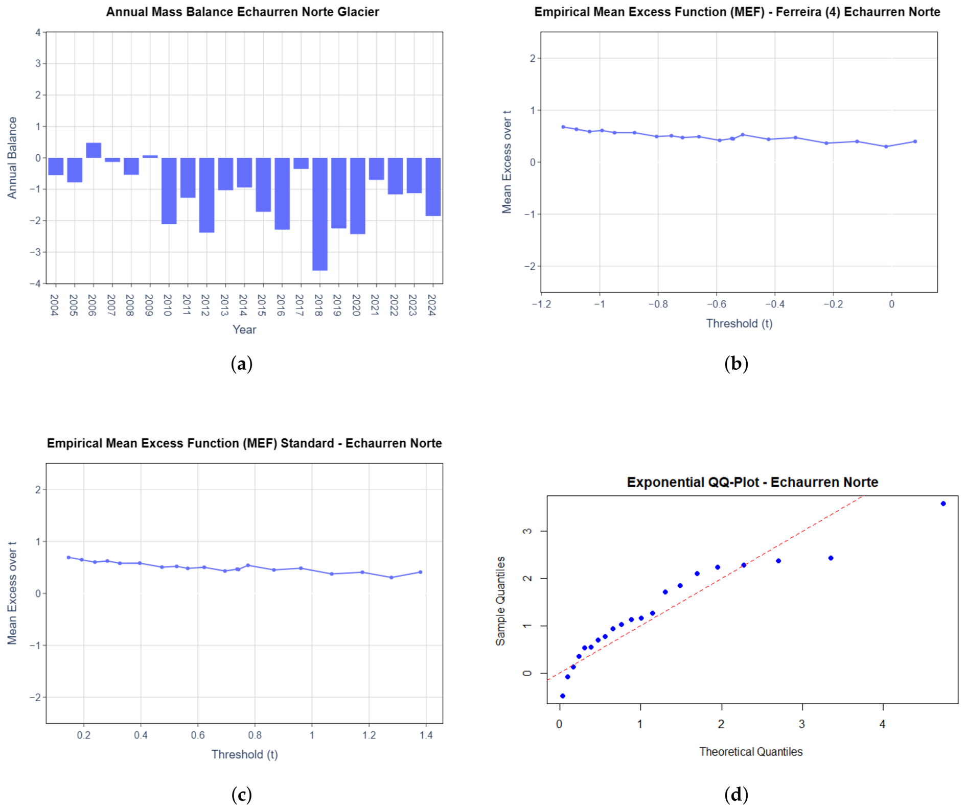
In Figure 2, the annual mass balance graph shows a sustained loss throughout the study period, particularly pronounced after 2010. Years with particularly intense losses are observed, such as the period 2007–2018, where a value close to −3.5 is reached, confirming the persistent retreat dynamics of this glacier.

The associated MEF exhibits a globally decreasing behavior as the threshold increases, indicating that the average excess decreases when only the most extreme events are considered. In this study, the median was selected as the base threshold, extending up to the 0.95 quantile. The curve does not show a clearly linearly increasing segment, suggesting that the distribution is not Pareto-type. However, a smooth modulation is observed between the approximate thresholds of 0.6 and 0.8, which corresponds to a curvature effect, with the negative slope being consistent with a slight or approximately exponential tail.

Furthermore, when applying the data standardization methodology proposed by [20], the shape of the original finite element is practically preserved, with no relevant structural changes evident. This indicates that the variability associated with time dependence does not dominate the behavior of the extremes, but rather that the tail structure is intrinsic to the series. The persistence of the decreasing slope reinforces the hypothesis of a weakly heavy or approximately exponential tail.

In the exponential QQ plot, the central quantiles show a reasonable fit with respect to the theoretical model; however, an upward curve appears in the upper quantiles, indicating that the extreme empirical values are larger than those expected under a purely exponential model. This suggests that the tail is slightly heavier than the exponential tail, although not extreme enough to be classified as Pareto, which is the regime of interest in this study.

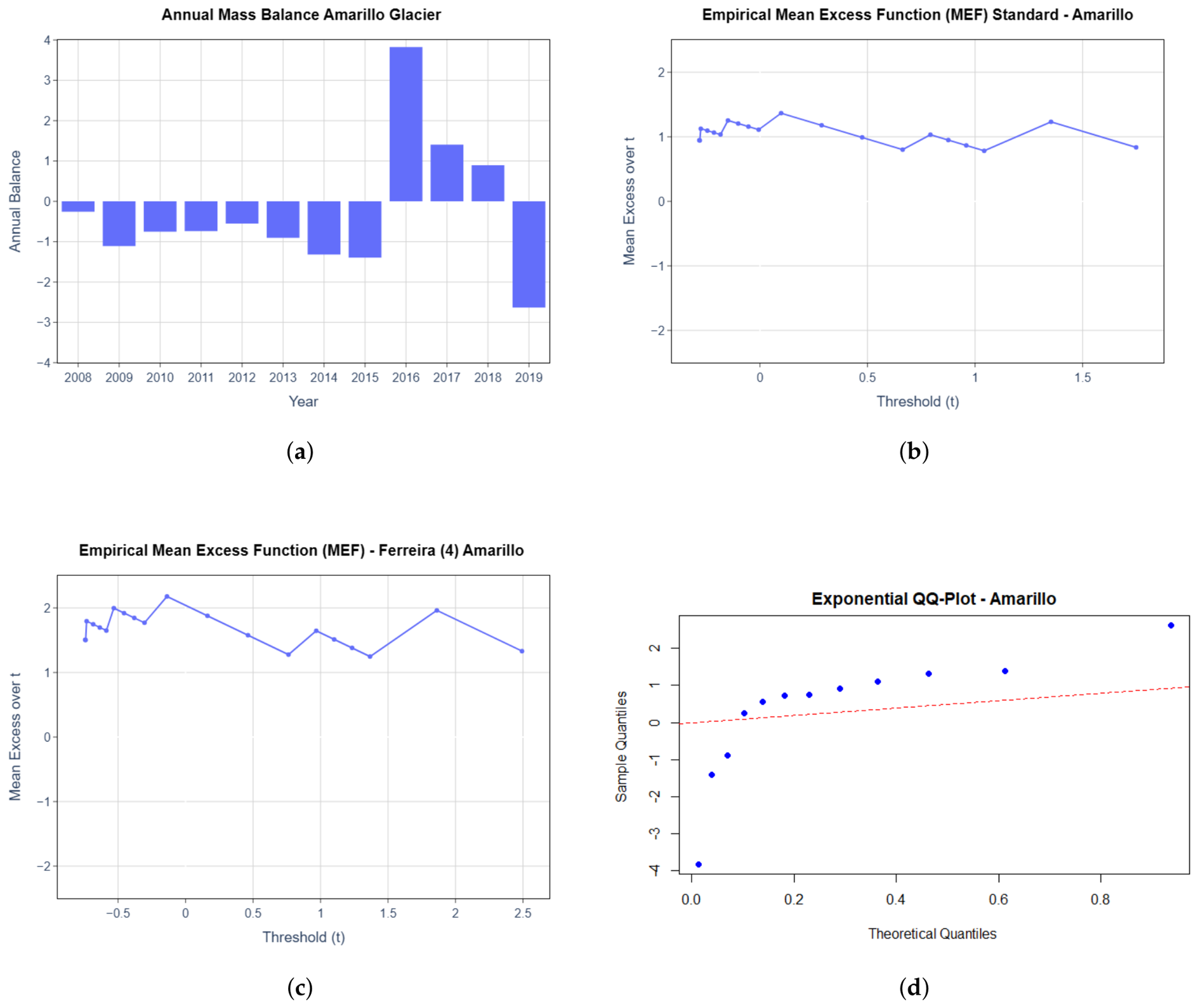
Figure 3 shows that the Amarillo Glacier gained mass during the period 2016–2018, significantly affecting the behavior of the mass flow curve (MEF) in both its standardized and non-standardized versions. While no significant structural changes are observed in the shape of the MEF, a relevant variation in its metric, as well as in the exponential QQ-plot, is evident. In certain sections, the MEF shows an increasing trend, which could be temporarily associated with Pareto-type behavior.

The annual mass balance of the Amarillo Glacier exhibits high interannual variability. During the initial period, negative values predominate, indicating a sustained loss of mass. However, from 2016 onward, significant positive values are recorded, notably an extreme event of approximately 4 m w.e., which clearly breaks the previous trend. Subsequently, the glacier again exhibits a marked loss around 2019. This behavior reflects a highly irregular dynamic, with alternating periods of extreme accumulation and abrupt losses.

The MEF of the Amarillo Glacier exhibits highly unstable behavior, without a clearly linear segment. Pronounced oscillations in the mean excess are observed as the threshold increases, with abrupt increases and decreases. This pattern suggests that the tail of the distribution does not clearly follow a Pareto-type structure, making it difficult to identify a stable extreme regime using the POT approach.

After standardization, the MEF maintains virtually the same erratic pattern observed in the original version, indicating that the instability is not due to a scale issue, but rather is intrinsic to the structure of the Amarillo Glacier’s extremes. The absence of a stable region reinforces the idea that there is no clearly optimal threshold for POT modeling under a classical GPD scheme.

The exponential QQ-plot of the Amarillo Glacier shows systematic deviations from the theoretical line, especially in the most extreme quantiles. In particular, empirical values are observed that deviate significantly from the expected behavior under an exponential model, including both negative and positive extreme events. This curvature confirms that the tail does not adequately follow an exponential distribution and that there are extreme events of considerable magnitude that are poorly represented by this model.

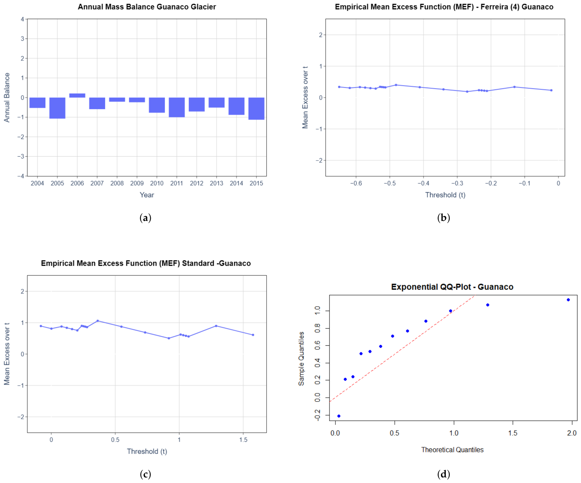
In Figure 4, corresponding to the Guanaco Glacier, the data collected between 2004 and 2015 show a clear predominance of negative values throughout the analyzed period, indicating a persistent and sustained loss of mass. The most critical years are concentrated approximately between 2005 and 2011. While there are some years with slightly positive or near-zero values, these do not offset the overall retreat trend, suggesting a relatively uniform behavior, without isolated extreme episodes like those observed in the Amarillo Glacier. The mean excess function (MEF) of the Guanaco Glacier is relatively stable, with a gently decreasing trend. A specific event is observed where the curve increases abruptly around the −0.3 threshold; however, in the standardized version, the overall shape of the MEF MFC TO MEF IN ALL plot is preserved, indicating that the tail is not dominated by scale effects. In this case, abrupt growth is observed around values close to one, suggesting a reasonable threshold range for POT modeling. Furthermore, no abrupt oscillations are observed, indicating that the excesses follow a regular pattern. This behavior is consistent with an exponential or weakly Pareto tail structure. The QQ-plot of the Guanaco Glacier shows good alignment of the empirical quantiles with the theoretical line, especially in the central and middle regions of the extremes. While there is a slight deviation in the highest quantiles, it is moderate and does not reflect a significant structural break, indicating that the exponential distribution is a reasonable approximation for describing the glacier’s extreme behavior.

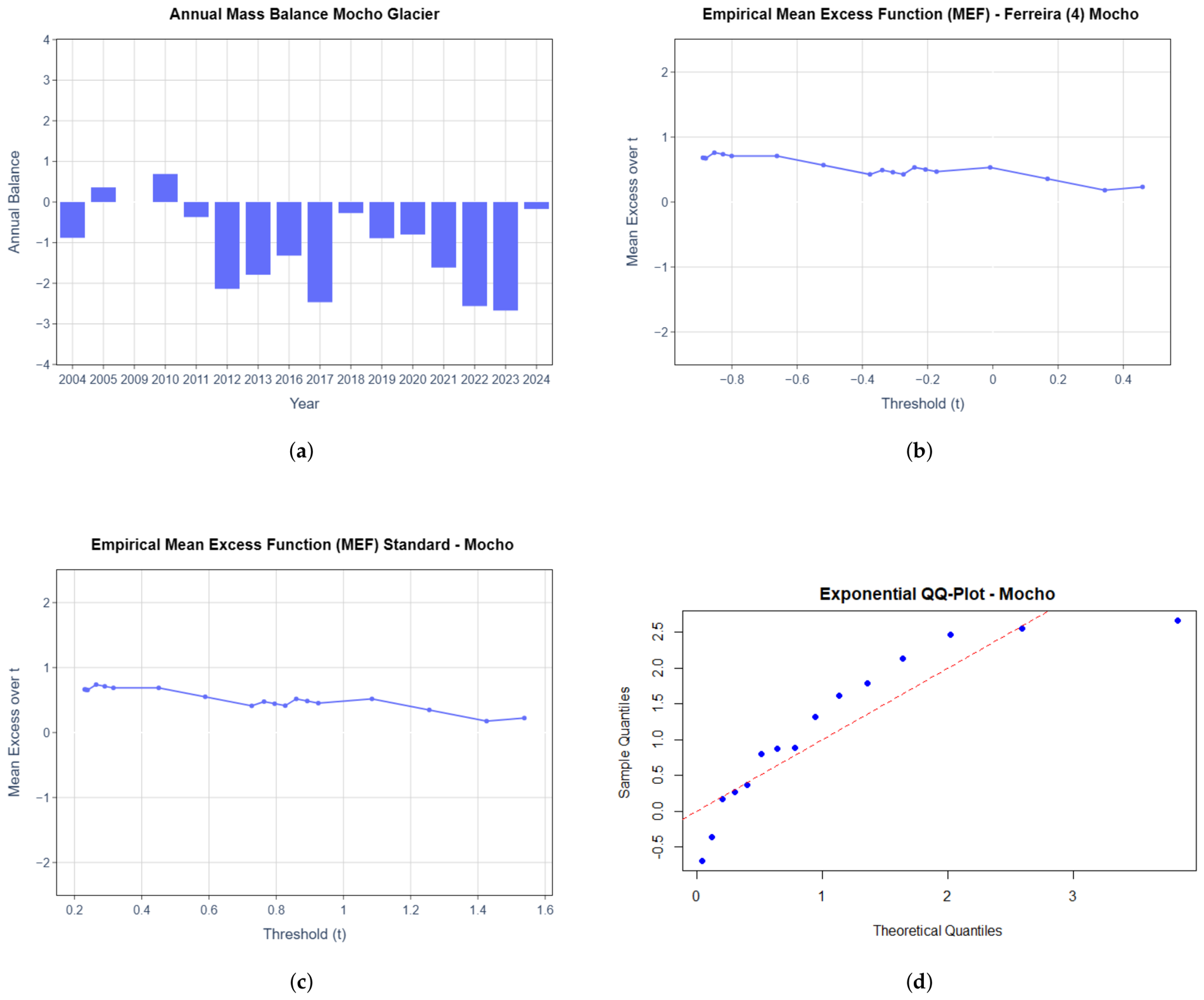
Figure 5 shows a break in the temporal continuity of the Mocho Glacier data, which is why the first two observations were discarded. Thus, the analysis window begins in 2011, from which point pronounced minima are evident in the final years of the record, with mass balance values close to −2.5. This behavior suggests an acceleration of glacial retreat in the final period of the analysis.

The MEF graph of the Mocho Glacier shows a globally decreasing trend as the threshold increases, indicating that average excesses decrease as more extreme events are considered. This pattern, as in the case of Echaurren Norte, is characteristic of a light or weakly heavy tail, without evidence of systematic linear growth that would indicate a heavily heavy tail. Although small intermediate oscillations are observed, the downward trend is clear.

After applying the standardization technique, as with the other glaciers, the decreasing structure of the MEF is preserved, reaffirming that the extremes are not dominated by scale effects. The persistence of the negative slope in both methodologies suggests that the glacier tail is structurally stable, with a progressive decay consistent with a slightly negative shape parameter.

To reinforce this result, the QQ-plot of the Mocho Glacier shows a good fit in the central quantiles with respect to the theoretical line. In the upper quantiles, a moderate positive deviation is observed, where the empirical values tend to be higher than the theoretical ones. This indicates that, while the tail is consistent with an approximately exponential behavior, there are moderate extreme events that contribute a slight additional heaviness, although not enough to classify the tail as strongly heaviest.

Taken together, these ME plots and MEF plots reflect a similar behavior to that observed in other environmental series reported in [20,22], especially regarding the effect of data standardization.

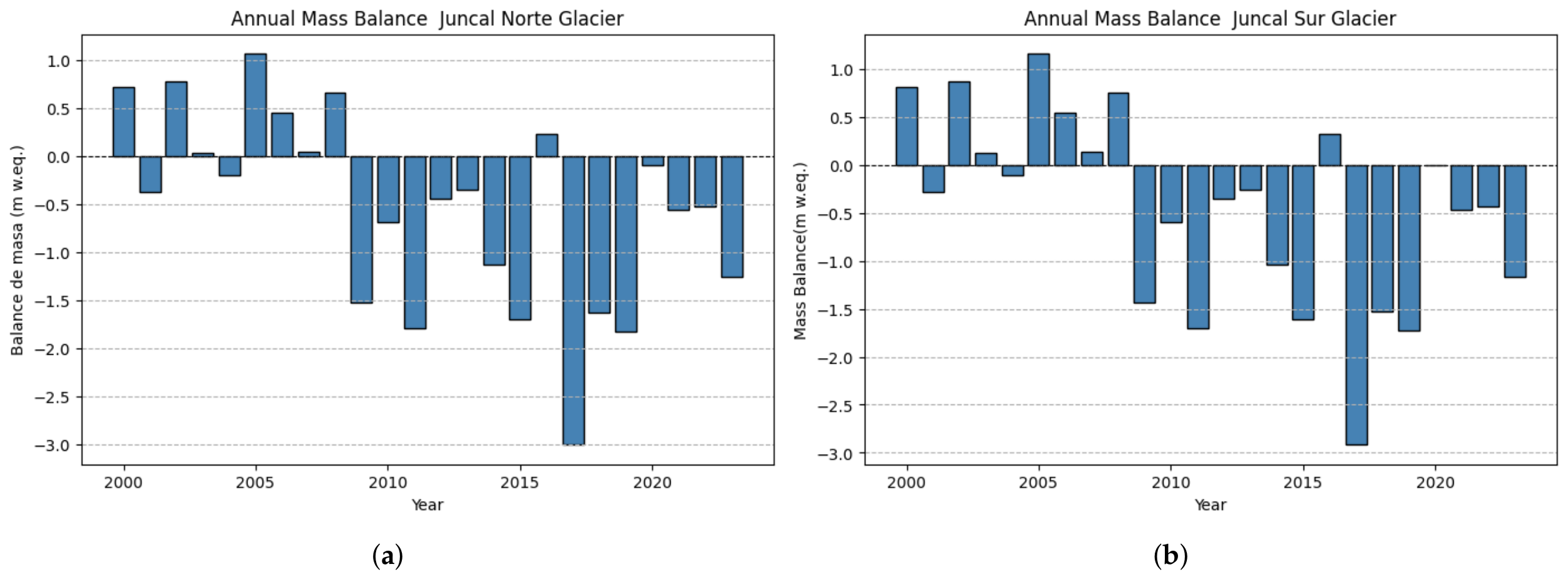
In Figure 6, the results for the Juncal Norte and Juncal Sur Glaciers show that both exhibit a negative trend in their annual mass balance, with a sightly bigger magnitude of loss in the Juncal Norte Glacier compared to Juncal Sur. This behavior is consistent with the historical evolution reported in [13].

These results agree with the evidence presented in recent studies [5], which indicate accelerated glacial melt in response to rising temperatures and decreased solid precipitation in central Chile. These conditions reinforce the high vulnerability of the analyzed glaciers and underscore their importance for environmental balance and the quality of life of the populations that depend on them.

The fact that the Echaurren Norte Glacier has a moderately heavy tail implies a relatively higher probability of severe extreme events compared to a purely exponential distribution. In practical terms, this means that episodes of very intense mass loss are not exceptionally rare events, but rather have a non-negligible probability of recurring. From the perspective of automated modeling, this characteristic increases uncertainty in extreme event prediction, since small variations in parameters can translate into large changes in extreme risk estimates, thus hindering the reliable projection of future extreme losses.

When comparing the two glaciers in the Atacama region (Guanaco–Amarillo), a contrasting behavior is observed. In the case of the Amarillo Glacier, unlike the other glaciers analyzed, the data show a positive increase in mass balance over the last five years, indicating episodes of extreme accumulation. In contrast, the Guanaco Glacier, as shown in Figure 4a), exhibits a sustained and persistent loss of mass throughout the study period, without episodes of significant recovery.

The main difference between the two glaciers lies in the thresholds identified through the Finite Element Method analysis. Specifically, the Amarillo Glacier shows a marked increase in the mean excess beyond the threshold near 0.5, especially in the unstandardized version of the model. In the standardized version, this behavior is similar in both the temporal and seasonal components, demonstrating a positive extreme response. Conversely, the Guanaco Glacier’s standardized model shows values around 1, while the unstandardized version ranges between approximately −0.3 and −0.1, reflecting a dynamic dominated by extreme losses rather than gains.

In this sense, it cannot be said that Guanaco is “more extreme” than Amarillo in absolute terms; rather, they exhibit different types of extremes: Amarillo concentrates positive extremes (abrupt gains), while Guanaco concentrates persistent negative extremes (sustained losses). Furthermore, Guanaco does not exhibit episodes comparable to the extreme gains recorded at Amarillo.

From a strictly statistical perspective, Amarillo Glacier can be considered the most vulnerable, as it displays the greatest instability in all extreme value diagnoses: a highly oscillating finite element MEF, a lack of stability in the variable-curve CV plots, and systematic deviations in the exponential QQ-plot. This instability prevents a robust characterization of its extreme regime under the POT-GPD approach, significantly increasing the uncertainty associated with predicting future extreme events. In contrast, glaciers such as Guanaco and Echaurren Norte exhibit much more stable tail structures, reducing the statistical uncertainty in their modeling.

Modeling Through EVT Techniques, Indirect Data

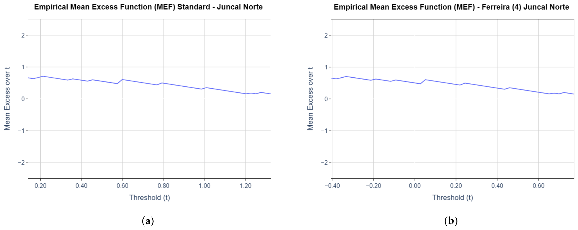
In Figure 7, corresponding to the indirect data, the behavior observed corresponds with the behavior in the direct data, specifically with Echaurren Norte. The behavior is equivalent to the one observed in the standardized function around that same point. This modeling suggests that indirect data complicate the direct application of GPD theory and, therefore, tend to generate a less stable generalization across the entire range of analysis.

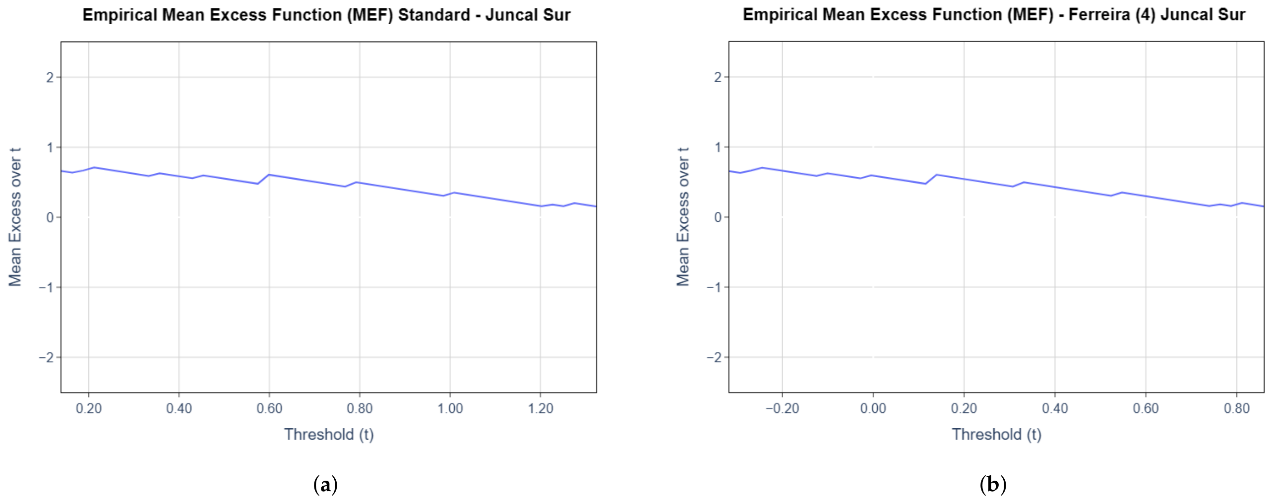
The same can be said in Figure 8. This behavior suggests that the theory is being applied well to this indirect data; however, caution is necessary in its use. It is worth noting that these data have already been studied and analyzed using similar approaches, as can be seen in the literature.

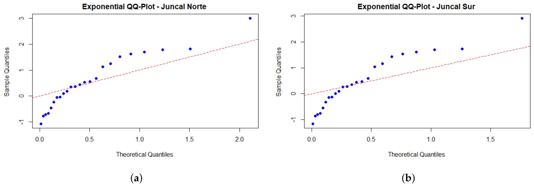
While the inclusion of the exponential QQ-plot is justified by the theoretical framework developed in the classical literature on extreme values, the data exhibit a different behavior compared to the previously analyzed glaciers, showing a curvature close to a logarithmic pattern. Although this behavior does not exactly match the theoretical exponential model, it does show a slight increase above the trend line, suggesting the presence of a heavy-tailed distribution in this case (Figure 9).

4.2. Perspective: Coefficients of Variance

Table 5 presents a summary of the main parameters obtained from the stability test of the coefficient of variation for the Amarillo, Echaurren Norte, Guanaco, and Mocho Glaciers. It can be observed that the thresholds defined from the median differ among glaciers, reflecting different scales in the magnitude of extreme losses. In particular, the Echaurren Norte Glacier presents the most negative threshold ($-1.12$), indicating greater severity in extreme events compared to the other glaciers, while Guanaco presents a less extreme threshold ($-0.65$).

The values of the $T_m$ statistic calculated in the $0.50$-to-$0.95$ quantile range show values close to zero for Guanaco ($-0.03$) and Amarillo ($0.04$), indicating good stability of the coefficient of variation in that threshold range. In contrast, Echaurren Norte and Mocho show values further from zero ($-0.26$), suggesting greater variability in the tail structure, although still compatible with a POT fit under a moderate stability framework. In all glaciers, $T_m$ values in the $0.95$-to-$0.99$ range are concentrated around $0.47$, indicating a loss of stability at the most extreme threshold levels, associated with the scarcity of available observations in those ranges.

Furthermore, when working with the absolute value of the data, the $T_m$ statistics show values close to $0.49$ for all glaciers, confirming that the structure of the extremes is consistent under both representations, although with limited stability in the higher quantiles.

Table 6. Summary of parameters per glacier.

Glacier	Threshold	Tm 0.5–0.95	Tm 0.95–0.99	TmAV	TmAV 0.95–0.99
Juncal Norte	$-0.09$	$-0.53$	$0.47$	$-0.5\phantom{0}$	$0.47$
Juncal Sur	$-0.02$	$-0.52$	$0.47$	$-0.5\phantom{0}$	$0.47$

, corresponding to the indirect data for the Juncal Norte and Juncal Sur Glaciers, shows that both have median thresholds close to zero ($-0.09$ and $-0.02$, respectively), indicating that the extreme events are of relatively lower magnitude compared to those of the glaciers analyzed using direct data. The $T_m$ values in the $0.50$-to-$0.95$ range are similar in both cases ($-0.53$ and $-0.52$), suggesting comparable extreme behavior between both glaciers at intermediate threshold levels.

However, when considering the most extreme range ($0.95$ to $0.99$), both glaciers exhibit a $T_m$ value of $0.47,$ again indicating a loss of stability at the upper extremes, consistent with observations in the CV-plots and tail estimators. Working with absolute values, the results remain stable for both glaciers, with $T_m$ approx. −0.50 and values close to $0.47$ in the upper quantiles, reinforcing the conclusion that the extremes in the indirect data exhibit a thinner and less stable structure than in the glaciers with direct measurements.

Overall, both tables show that the stability of the coefficient of variation is reasonable in intermediate quantile ranges, but it systematically degrades at the most extreme levels (0.95–0.99), which is consistent with the decrease in the effective sample size and the greater uncertainty in the tail estimation. These results reinforce the need to interpret extreme parameters at higher threshold levels with caution, especially in the case of indirect data.

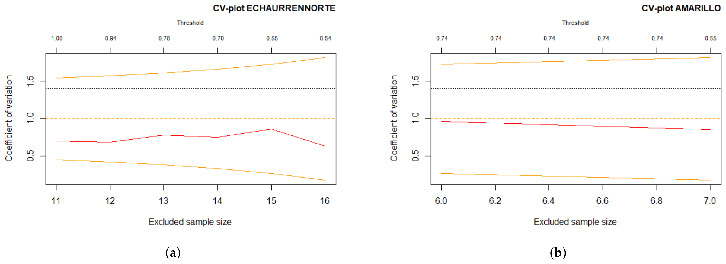
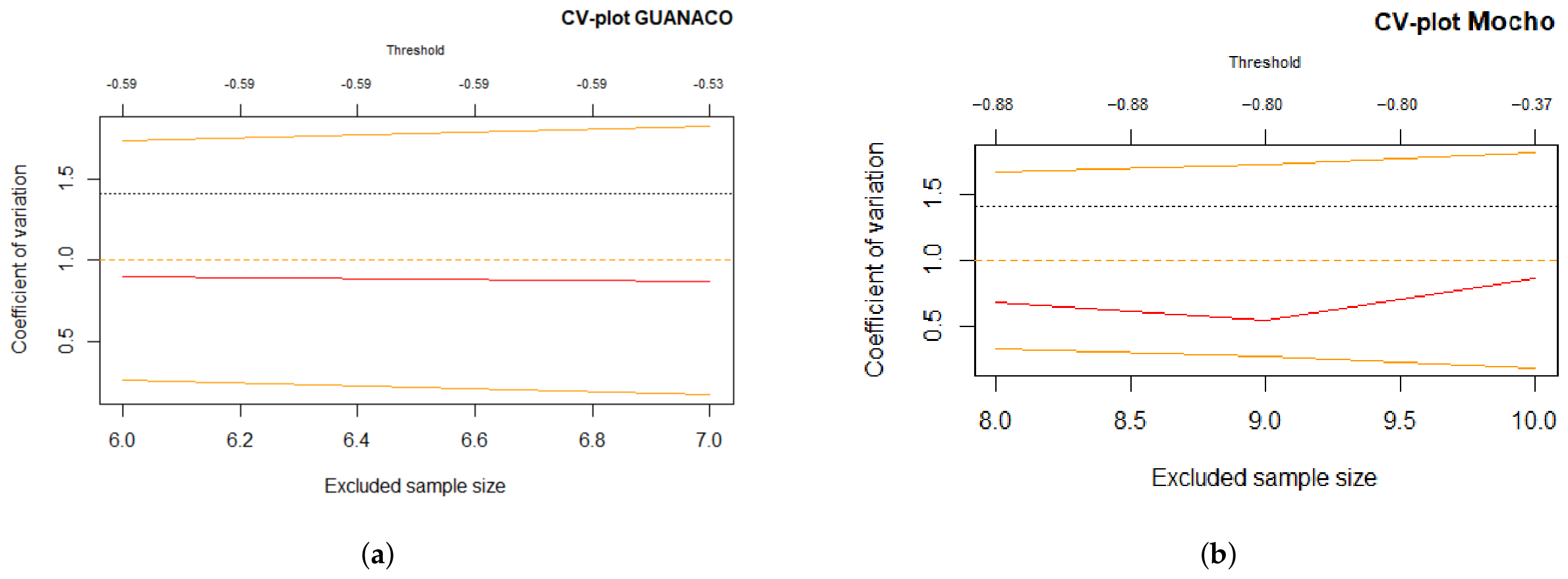
Applying the CV-plots reveals that all datasets remain within the confidence bands, providing an initial visual indicator of stability, albeit a descriptive one. None of the graphs systematically exceeds the central reference line. In particular, the Amarillo (Figure 10) and Guanaco (Figure 11) Glaciers show the best alignment with this reference, while stability is less pronounced in the other cases.

In the case of the Amarillo (Figure 10) Glacier, the coefficient of variation for excesses remains around 0.8–0.9, with a slight upward trend as the size of the excluded sample or the threshold increases. While the curve does not exhibit abrupt oscillations, it also does not show a clearly stable region, indicating that the structure of the extremes does not fully consolidate under the POT approach. Indeed, the values remain below the reference CV = 1, suggesting that the tail is not heavy, but rather weakly extreme. Furthermore, although the empirical curve remains within the confidence bands, the absence of a flat window reinforces the results previously obtained from the MEF and the exponential QQ-plot, highlighting the high irregularity in the extreme behavior of this glacier. In this context, the approximate threshold range between −0.74 and −0.55 cannot be considered an optimal interval with full statistical certainty, due to the marked lack of stability. Consequently, the CV-plot confirms that the Amarillo Glacier has a non-heavy, likely constrained, tail with poor stability at the extremes, which implies that fitting a GPD under the POT approach should be done with particular caution.

In the CV-plot of the Echaurren Norte Glacier (Figure 10), the curve is not perfectly straight across the different thresholds, showing a slight increase in the approximate range between −0.94 and −0.55. However, the coefficient of variation remains relatively stable across the excluded sample sizes considered, approximately between 11 and 6 observations. This stability is the main indication that the tail structure does not change abruptly when the threshold varies. Furthermore, the values remain below the reference CV = 1, which corresponds to behavior close to the exponential case, suggesting that the tail is not extremely heavy, but rather light. In addition, the empirical CV curve remains within the confidence bands throughout the analyzed range, allowing us to conclude that no significant structural deviations are detected in the excess behavior. Consequently, the CV-plot confirms that the Echaurren Norte Glacier has a stable, non-heavy tail, consistent with a GPD model, validating the use of the POT approach in this case.

The CV-plot for the Guanaco Glacier (Figure 11) remains practically straight, meaning the coefficient of variation is remarkably stable across the entire range of analyzed sample sizes and, consequently, across the different thresholds. The values remain close to 0.9, with very low variability, which is clear evidence of high stability in the tail. In this case, the values are slightly below one, indicating that the tail of the distribution is not heavy, but rather exhibits behavior very close to exponential. Furthermore, the empirical curve remains entirely within the confidence bands, showing no structural changes, thus reinforcing the robustness of the diagnosis. The threshold range approximately between −0.59 and −0.53 can be considered an optimal interval for threshold selection, as it clearly meets the stability condition.

Overall, the application of the CV-plot confirms that the Guanaco Glacier exhibits a highly stable, non-heavy tail that closely approximates the exponential case, strongly supporting the use of the POT approach with a GPD for modeling its extremes. Within the set of glaciers analyzed, Guanaco stands out as the most stable and statistically reliable case from the perspective of Extreme Value Theory.

For the Mocho Glacier (Figure 11), the coefficient of variation of the excess remains relatively constant across the excluded sample size range of approximately 8 to 10 observations. CV values range from 0.75 to 0.90, with a slight upward trend at higher thresholds, indicating moderate but controlled variability in the tail. Furthermore, the values remain below the reference CV = 1, suggesting that the tail is not heavy but exhibits behavior close to the exponential case. The empirical curve remains within the confidence bands, showing no evidence of significant structural breaks. The total range of associated thresholds is approximately between −0.48 and −0.37, which can be considered a suitable interval for threshold selection. This technique again confirms that the Mocho Glacier has a stable tail, with slightly lower stability than that observed in the Guanaco Glacier, but clearly higher than that of the Amarillo Glacier. In terms of the GPD shape parameter, this pattern is consistent with a value close to zero or slightly negative.

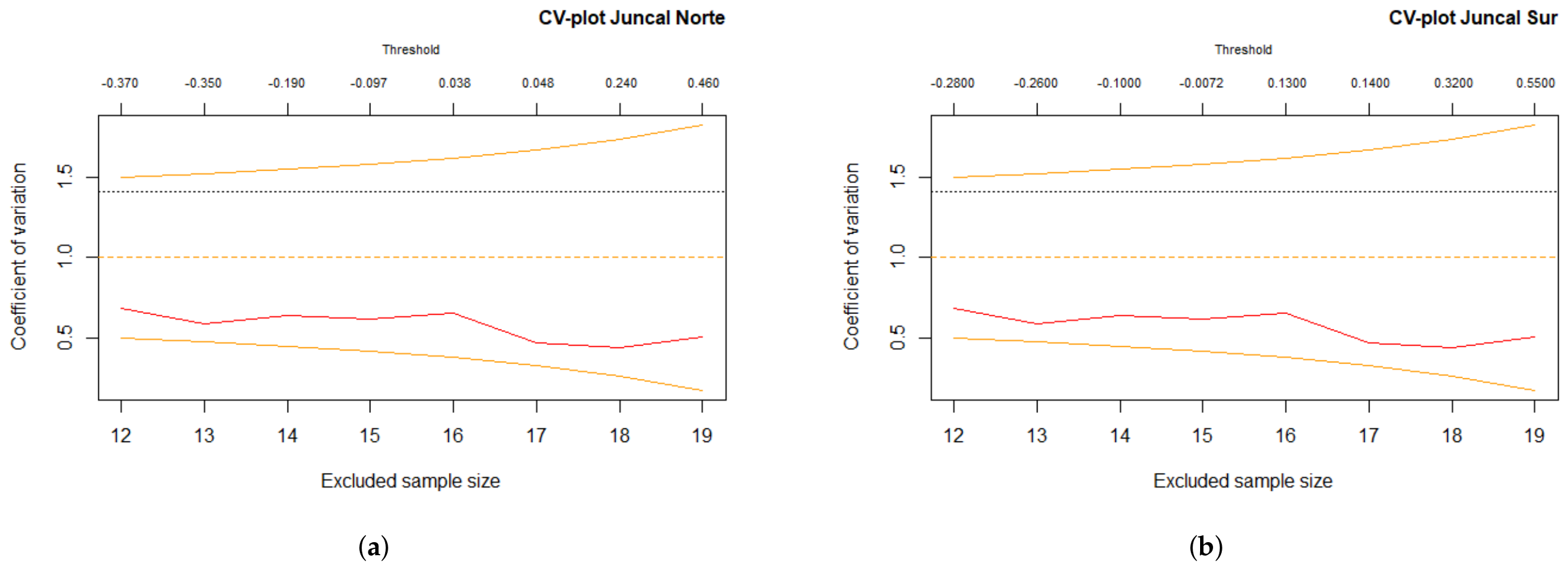
Now, in the analysis of the indirect data, it is observed that the Juncal Norte Glacier (Figure 12a) exhibits a roughly constant decrease in the coefficient of variation, with small windows of increase, showing a behavior very similar to that of the Juncal Sur Glacier (Figure 12b). In particular, the CV-plot of Juncal Norte shows a clearly decreasing trend as the threshold or size of the excluded sample increases, falling from values close to 0.8–0.9 to values close to 0.4. This indicates that the relative variability of the excesses decreases progressively as the focus shifts to the most extreme events.

Furthermore, these values always remain below the reference CV = 1, which suggests that the tail of the Juncal Norte Glacier is not heavy, but rather quite thin. In addition, the empirical CV curve remains within the confidence bands without showing abrupt changes; however, a clearly horizontal region of stability, as seen in the previously analyzed glaciers, is not observed. This suggests that, while the POT approach is applicable, the selection of the threshold should be done with particular caution, prioritizing intermediate values before the steepest drop.

Similarly, the Juncal Sur Glacier exhibits a behavior in which the coefficient of variation again shows a progressively decreasing trend, going from values close to 0.8–0.9 to values close to 0.4–0.5 at the highest thresholds. This pattern indicates a systematic reduction in the relative variability of the excesses, characteristic of distributions with thin tails. Again, the values remain below the exponential threshold (CV = 1) and within the confidence bands, without evidence of significant structural breaks. However, the absence of a clearly stable section limits the identification of an optimal POT threshold with high robustness.

The combined analysis of the glaciers using the extreme value approach and the POT/GPD methodology allows us to conclude that the Guanaco Glacier is the most statistically robust case, due to its highly stable tail structure and the good agreement observed in the exponential QQ-plot with the theoretical model, solidly validating the application of this approach. The Echaurren Norte Glacier exhibits a stable tail, although with slightly greater variability than Guanaco. The combination of a decreasing MEF, an exponential QQ-plot with moderate curvature in the upper quantiles, and a stable CV-plot below unity indicates a non-heavy tail, slightly lighter than that of the exponential model. In this case, the POT approach is suitable within the identified threshold range, although less robust than in Guanaco.

In contrast, the Amarillo Glacier exhibits the most unstable and complex behavior of all the cases analyzed. Its mass balance shows an alternation between extreme losses and gains, resulting in a highly oscillating finite element mass without clear periods of stability. The exponential QQ-plot shows significant deviations, and the CV-plot does not exhibit a uniform pattern or a well-defined stable region. Taken together, these results indicate that the Amarillo Glacier does not fit well to a classic Pareto or exponential model, so the POT/GPD fit should only be performed under strict empirical validation of stability at the extremes.

Finally, the Juncal Norte and Juncal Sur Glaciers exhibit clearly different behavior from the rest. Since these correspond to indirect data, they should be analyzed with particular caution. In both cases, the CV-plots show a systematic decrease in the coefficient of variation as the threshold increases, reaching values close to 0.4. This pattern is characteristic of light and potentially constrained tails. Furthermore, the absence of large regions of stability suggests that, while the POT approach is applicable, the selection of thresholds is particularly sensitive, limiting the robustness of the GPD adjustment in these glaciers.

4.3. Estimators for Tail Behavior

The Hill, t-Hill, and Zipf estimators allow for the analysis of the left tail of the glacier’s annual mass balance, quantifying the magnitude of extreme declines. In the corresponding graphs, the horizontal axis represents the number of extreme values considered (k), and the vertical axis shows the tail index estimate (${\widehat{\gamma }}_k$). A range of k values within which the estimators remain relatively constant indicates a reliable estimate of the $\gamma$ parameter.

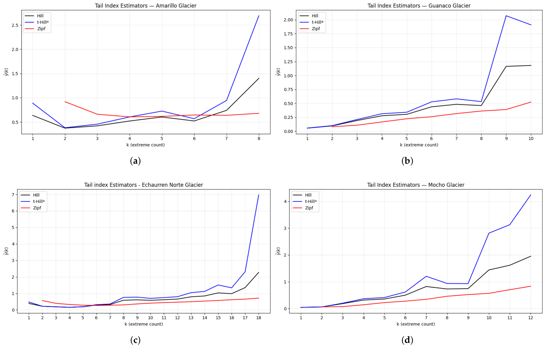
In the analysis of the tail index for the Amarillo Glacier (Figure 13), the three estimators exhibit similar behavior, suggesting that the estimates are not strongly affected by extremely outliers. However, the lack of convergence indicates the absence of a robust region of stability, confirming that the Amarillo Glacier’s tail does not correspond to a well-defined extreme model. For small values of k, the three estimators show low and similar values, indicating the presence of a moderately heavy tail. From $k\approx 7$, the t-Hill estimator exhibits abrupt growth, reaching significantly higher values than the Hill and Zipf estimators. This behavior suggests a high sensitivity of the t-Hill estimator to severe extreme values, confirming the presence of large-magnitude mass loss events in this glacier. The Zipf estimator remains consistently lower, providing a more conservative estimate of the tailing index. These results are entirely consistent with previous observations in the MEF and CV-plot, where no stable extreme behavior is identified either. Consequently, the tailing index estimate for Amarillo should be interpreted with extreme caution.

Figure 13, which forms part of the motivation for this work based on [15], shows a progressive and stable increase in the tail index as k increases, with a clear intermediate zone of stability. In this study, a different criterion was adopted than in the cited work, considering $k_{\max }=n-1$, where n corresponds to the number of negative observations of the Guanaco Glacier. The estimated values remain around low to moderate levels, which is consistent with an approximately exponential or slightly heavy tail. In this glacier, the three estimators show increasing and relatively stable behavior up to approximately $k=7$, indicating a suitable stability range for estimating the tail index. From $k=8$, the t-Hill estimator shows an abrupt increase, while Hill increases more moderately. This result is consistent with that reported in [15], where $k=7$ is identified as an optimal value for this glacier. The Zipf estimator maintains a smooth increasing trend, confirming the existence of a heavy tail with less variability. This result reinforces the conclusions obtained previously, where Guanaco was identified as the most stable and robust case for the proposed model.

Figure 13 shows a sustained increase in the tail index with increasing k, accompanied by an intermediate zone where the estimators are relatively stable. This behavior indicates that the Echaurren Norte Glacier has a moderately heavy tail, more intense than that of Guanaco, although without reaching an extreme heaviness regime, consistent with previous diagnoses. However, this glacier exhibits the most unstable behavior among the four analyzed. For small and medium values of k, the estimators remain close to zero, suggesting that extreme losses are infrequent or of moderate magnitude. However, starting at $k\approx 17$, the t-Hill estimator shows explosive growth, far exceeding that of Hill and Zipf. This demonstrates the presence of extremely atypical tail values, which generate significant instability in the tail index estimation when too many extreme observations are included.

Finally, for the Mocho Glacier (Figure 13), patterns similar to those at Echaurren Norte are observed, but with a steeper slope for high k values. This indicates the presence of a moderately heavy tail, with a greater influence of extreme events compared to Guanaco, although without reaching the level of instability observed at Amarillo. This result is consistent with previous observations from the other diagnostic methods. For the Mocho Glacier, a progressive evolution of the tail index is observed for all three estimators up to approximately $k=7$. From this point, the t-Hill estimator begins to clearly diverge from Hill and Zipf, and from $k\approx 9$ it shows an abrupt increase, reaching values greater than $\widehat{\gamma }=3$. The Hill estimator increases more moderately, while Zipf maintains a gentle slope. This behavior indicates the presence of a very heavy tail, associated with severe extreme losses in certain years.

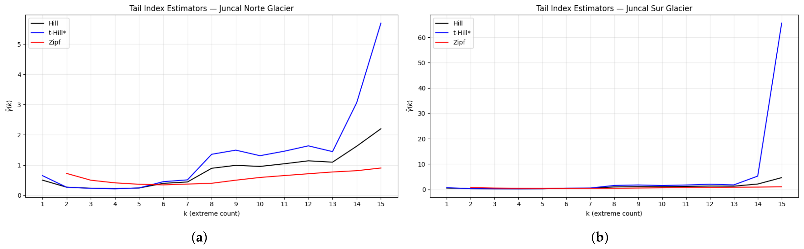
Figure 14 shows a very similar behavior between Juncal Norte and Echaurren, which in turn shows that the glaciers have a moderately heavy tail like Mocho; there is a distinct flatness in $k=6$ just like in Echaurren. Meanwhile, for Juncal Sur, for large values of k, the estimator t-Hill experiences an abrupt increase, which is comparable to that of Juncal Norte. This divergence is indicative of instability in the tail index estimation, usually associated with a scarcity of effective extreme data or the presence of very isolated events that dominate the estimation.

The comparative analysis of the glacier group confirms that the Guanaco Glacier stands out as the most stable and statistically robust case, where the estimators exhibit a coherent and stable evolution of the tail index, with low and consistent values. Echaurren Norte, for its part, presents a stable tail structure, although with greater variability than Guanaco, showing an intermediate region of reasonable stability. In the case of the Mocho Glacier, the estimators increase steadily with a slight relative heaviness compared to Guanaco, while the Zipf estimator maintains a gentler slope.

Finally, the Amarillo Glacier exhibits unstable behavior, as the estimators show strong variability without convergence. Regarding indirect data, the glaciers display clearly distinct behavior, with low tail index values and no large regions of stability. In particular, at Juncal Sur, the abrupt increase in Hill and t-Hill values for large k values is mainly due to a scarcity of effective extremes and not necessarily to the presence of a truly heavy tail, which is consistent with the behavior observed in the CV-plots.

In practical terms, a moderate ${\widehat{\gamma }}_k$ value indicates that extreme mass declines are not excessively heavy, although extreme events of significant magnitude do occur.

From the joint analysis using MEF, exponential QQ-plots, CV-plots and the Hill, t-Hill and Zipf estimators, the regime of the shape parameter $\gamma$ was identified for each glacier, which is summarized in

Table 7. Classification of shape parameter $\gamma$ by glacier.

Glacier	Tail Regime	Interpretation of $\mathsf{\gamma }$
Guanaco	Stable exponential	$\gamma \approx 0$
Echaurren Norte	Exponential/light	$\gamma \approx 0$ or $\gamma <0$
Mocho	Light	$\gamma \lesssim 0$
Amarillo	Unstable	$\gamma$ not identifiable with stability
Juncal Norte	Light and bounded	$\gamma <0$
Juncal Sur	Light and bounded	$\gamma <0$

.

For the Guanaco Glacier, the MEF, CV-plot, QQ-plot, and Hill estimators indicate an approximately exponential tail, so the shape parameter is classified as $\gamma \approx 0$. For the Echaurren Norte Glacier, the stability observed in the CV-plot with values below one, along with a decreasing MEF, suggests a light tail, consistent with a $\gamma \approx 0$ or slightly negative value. The Mocho Glacier exhibits a clearly decreasing MEF and a CV below one, indicating a light tail, associated with a $\gamma \lesssim 0$ shape parameter.

For the Amarillo Glacier, no stable region of the tail index is identified in any of the diagnoses used, so it is not possible to assign a reliable value to $\gamma$ within the POT/GPD framework.

Finally, the Juncal Norte and Juncal Sur Glaciers exhibit decreasing CV-plots with values well below unity, consistent with slight and potentially constrained tails, implying a strictly negative shape parameter, $\gamma <0$.

This study provides a clear statistical characterization of the extreme behavior of the analyzed glaciers and how they respond to extreme mass loss or gain events, as evidenced particularly in the Amarillo Glacier. The analyzed series present distinct geomorphological, climatic, and topographic conditions, such as differences in altitude, aspect, cover, and accumulation regime, resulting in heterogeneous extreme responses. In this context, the results should be interpreted considering that glacial behavior is not uniform, especially in a future scenario where the availability of water resources is not guaranteed. From an environmental perspective, it is important to emphasize that glaciers should be understood not only as water reservoirs but also as fundamental ecosystems within the climate system. While the main focus of this study was on water resources, it is important to highlight that these ice masses constitute an essential component of biodiversity and environmental balance in central Chile.

Furthermore, among the main limitations of this study is, firstly, the existence of different sample sizes among glaciers, which can affect the stability and comparability of the shape parameter $\gamma$ estimates, especially in cases with fewer extreme observations. Secondly, the analyzed data come from indirect mass balance estimates, which are subject to measurement noise and instrumental uncertainty, which can propagate into the extreme value analyses. Likewise, the potential temporal dependence between observations constitutes a significant limitation, since Extreme Value Theory, in its classical formulation, assumes independence between data. Finally, the results of the POT/GPD approach are sensitive to the threshold selection, so an inappropriate choice can introduce biases into the $\gamma$ estimate and compromise the robustness of the conclusions.

5. Conclusions

This chapter synthesizes and integrates the main results obtained throughout the study, aiming to establish a comprehensive interpretation of the extreme mass balance behavior of the analyzed glaciers. Specifically, the study sought to determine the nature of their distribution tails, evaluate the suitability of the Peaks Over Threshold (POT) approach with adjustment using the Generalized Pareto Distribution (GPD), and establish comparisons between glaciers based on objective criteria of statistical stability.

In particular, this study analyzed the extreme mass balance behavior of the Guanaco, Echaurren Norte, Mocho, Amarillo, Juncal Norte, and Juncal Sur Glaciers using Extreme Value Theory (EVT) tools, under the Peaks Over Threshold (POT) approach and adjustment using the Generalized Pareto Distribution (GPD). The suitability of the model was evaluated through the Mean Excess Function (MEF), exponential QQ-plots, CV-plots and Hill, t-Hill and Zipf tail estimators, allowing a comprehensive characterization of the extreme distribution of each glacier.

5.1. Analysis of Extreme Behavior and Validation of the POT/GPD Approach

First, the suitability of the POT/GPD approach for modeling the extreme mass balance of the Guanaco, Echaurren Norte, Mocho, Amarillo, Juncal Norte, and Juncal Sur Glaciers was analyzed using Extreme Value Theory (EVT) tools, specifically the mean excess plot (MEP) with an addition specified in [17]. This analysis aimed to evaluate whether excesses above a certain threshold—in this case, the median, due to the nature of the data, where any behavior outside this ’normal’ raises concerns and triggers changes in reality—could be adequately represented by a mean excess plot (MEP), a fundamental requirement for extreme inference.

The MEP analysis, along with the mean squared error (MSE) of the linear fit, revealed clear differences in extreme behavior among the glaciers. The Guanaco Glacier showed the best fit with an approximate MSE of 0.0018, indicating a highly stable tail structure and excellent agreement with the GPD. It was followed by the Mocho Glacier with an MSE of 0.0033, also demonstrating robust behavior. The Echaurren Norte Glacier showed a moderate fit with an MSE of 0.0128, reflecting an acceptably stable tail, although with greater variability. In contrast, the Amarillo Glacier presented the worst performance with an MSE of 0.0451, indicating a non-linear MEF, associated with an unstable extreme structure and high interannual variability.

5.2. Characterization of Tail Type and Extreme Stability in Glaciers Using Direct Data

Once the general applicability of the approach was validated, the tail type and degree of extreme stability in glaciers were characterized using direct data, with the aim of establishing their dominant extreme regime and the reliability of the modeling.

The results show that the Guanaco Glacier exhibits sustained and regular mass loss, with a stable finite element mass, a practically constant CV-plot (i.e., a straight line) along the different thresholds, and an exponential QQ-plot with good theoretical agreement, indicating an approximately exponential tail and a shape parameter $\gamma \approx 0$, which reinforces the theory of being approximately exponential. The Echaurren Norte Glacier also exhibits a stable tail, although with greater variability, consistent with an exponential or slightly thinned distribution. In the case of the Mocho Glacier, an intermediate behavior is observed, with a decreasing MEF, a CV less than one, and a slight positive deviation in the QQ-plot, suggesting a tail close to the exponential case with a slight influence of moderate extremes.

Conversely, the Amarillo Glacier exhibits the most unstable behavior of the group, with alternating severe losses and extreme gains, a highly oscillating MEF, a lack of stability in the CV-plot, and marked deviations in the exponential QQ-plot. In this case, it is not possible to identify a well-defined extreme regime under the POT/GPD approach, so the estimation of the shape parameter $\gamma$ must be interpreted with extreme caution, significantly increasing the uncertainty associated with predicting future extreme events.

5.3. Glacier Analysis with Indirect Data and Its Statistical Implications

Subsequently, the extreme behavior of the Juncal Norte and Juncal Sur Glaciers, constructed from indirect data, was analyzed to evaluate the extent to which this type of information affects the stability of the EVT diagnoses and the robustness of the extreme modeling.

The Juncal Norte and Juncal Sur Glaciers, corresponding to indirect data, exhibit clearly decreasing CV-plots and values well below one, indicating slight and potentially bounded tails, associated with a Weibull or Gumball distribution shape according to the theory presented in Section 2.4. Although the POT approach is applicable in these cases, the absence of broad regions of stability limits the robustness of the GPD fit and requires special caution in the selection of the threshold, due to the sensitivity of the results to small variations in the available extremes.

As previously discussed, the comparative analysis concludes that there is no homogeneous extreme behavior among the glaciers analyzed, even within the same geographic region, as in the case of the Guanaco and Amarillo Glaciers in the Atacama Desert. This highlights the need for individualized extreme glacial value (EVT) studies. From a hydrological and climatic perspective, these results confirm the high vulnerability of glaciers in central Chile to rising temperatures and decreased solid precipitation, reinforcing their critical role in regulating water resources. In this context, glaciers should be understood not only as strategic water reserves but also as fundamental ecosystems for environmental stability.

Finally, this study provides a solid statistical basis for modeling extreme events in Chilean glaciers, constituting a relevant input for future hydroclimatic projections, risk studies, and water resource management planning under a climate change scenario. Furthermore, the results obtained open the possibility of extending this approach to non-stationary models, the incorporation of climatic covariates and the use of regional climate change projections to strengthen the assessment of extreme risk in glacial systems.