Cost-of-Quality Study for NC Water Utilities Using the Hickory Municipal Classification System

Abstract

The growing expectation of citizens to deliver quality services without increasing taxes requires municipalities to adjust their cost models to remain good stewards of the voters’ finances. Cost-of-Quality (CoQ) models have traditionally been studied in relation to manufacturing processes as a method to increase profitability by reducing the life-cycle costs of the product. Municipalities have historically not been included in these studies as they operate on a semi-monopolistic basis for the services and infrastructure they maintain and have a different set of constraints and obligations from private entities. An analysis of three North Carolina municipalities (Winston-Salem, Cary, and Apex) is conducted to evaluate the Cost-of-Quality components of their water system budgets. The analysis consists of two evaluations. The initial evaluation compares the budgets of the aforementioned North Carolina municipalities with a previous study that analyzed three Texas municipalities’ water system budgets (Lubbock, San Antonio, and El Paso). The purpose of this portion of the study is to evaluate whether North Carolina Cost-of-Quality components behave like Texas municipalities. The second portion of this study evaluates the three North Carolina municipalities independently of the Texas study to see whether population size is a differentiator in how Cost-of-Quality components are divided in North Carolina. The three NC municipalities are chosen based on the Hickory Municipal Classification System (MCS). The Hickory MCS is a national classification system based on the relative population of each state and was developed for this study. The Texas municipalities that were studied had variable populations, variable locations, variable water sources, and variable water uses. The Cost-of-Quality analysis focuses on prevention costs, appraisal costs, failure costs, Total CoQ costs and opportunity costs between the North Carolina and Texas municipalities. Of the twelve comparative hypotheses, three CoQ costs are found to be significantly different with a probability level of p < 0.05. The results suggest that appraisal and failure costs are consistently impactful across the utilities in both states, but opportunity costs are not materially significantly different as in previous studies on Cost of Quality for utilities.

1. Introduction

The Costs of Quality is the lost value of a system that is associated with poor performance of products, services, and processes including the costs for not meeting customers’ requirements, expectations or needs [1] (p. 150). This “lost value” is not a minor cost and has been shown to account for up to 30% of all costs of the system. Therefore, by focusing on systemic quality of a system, quality may be improved with an additional benefit of a decrease in cost of the system [1].

Cost of Quality was first introduced by Juran in 1951 when he reasoned that good quality for a company’s product may not be enough to ensure the company’s survival, but with low quality, that business was sure to fail [2]. Juran argued that for a product’s life cycle, there was an optimum to the quality of design. Above this optimum point, to become known as the “Juran Point,” the cost to achieve a better design is not paid back by the value brought by the market. Alternatively, the savings of designing a product to less-than-optimum quality are smaller than the realized market value if designed to the Juran Point [2] (p. 6).

There were several additions to Juran’s original CoQ model, but it was not until 1992 that Lawrence Carr modified the existing CoQ models to account for the Service Industry, which, up to this point, was developed and focused on manufacturing [3]. Carr’s service inclusion helped lay the groundwork for Banasik’s & Beruvides’ research [4], which utilized the CoQ model for municipal infrastructure. The history of how municipalities regulate infrastructure may also help shape public opinion on their operation, as is explained as follows: “A major segment of political government regulation has been to protect the safety and health of its citizens. At the outset, the focus was on punishment ‘after the fact’—the laws provided punishment for those whose poor quality had caused death or injury. Over centuries there emerged a trend to regulation ‘before the fact’—to become preventive in nature.” [1] (p. 55).

Water and sewer utilities may also face a unique vicious cycle while ensuring that service levels are maintained. For instance, a Public Utility may propose expansion of capability based on current usage and projected growth. Once loans/bonds are exercised to build this infrastructure, any lowering of income creates hardship for the utility. The cycle could begin during a drought where restrictions are placed on citizens to reduce water. Either through habits or technology, the baseline for water use may be reduced permanently, which reduces income. The response of the utility may be to raise rates to compensate for the lost income. As Arrandale wrote, quoting Mary Tiger, chief operating officer at the University of North Carolina Environmental Finance Center, “Raising rates to catch up, however, just gives customers more reason to use less water. That reduces water sales even more, and water supply agencies ‘end up in a downward cycle of lower revenues and increasing rates, and customers feel like they’re being punished for doing the right thing,” [5] (p. 42). As an example, the utility in Wichita Falls, Texas, lost $4.5 million in revenue in 2013 after drought forced it into drastic water-saving steps [5]. The option of raising rates for a utility is therefore not the first or most ideal option. The second option therefore is to reduce the cost of operation and maintenance or minimize a rate increase. To ensure consistency in terminology across the study, key operational definitions are provided in Appendix A.

1.1. Challenges with Public Infrastructure Management

In 2013, two examples of forcibly privatizing public infrastructure in North Carolina included (1) the NC Senate’s attempt to remove the City of Charlotte’s control over “Charlotte Douglas International Airport” and give control to a regional authority [6] and (2) the NC House’s attempt to remove the City of Asheville’s control of its own water system and again put it under a regional board [7]. In addition to authorities taking over assets and infrastructure through legislation, there is also an opportunity for private entities to build competing infrastructure, as was the case for the Public–Private Partnership (PPP) involving the construction of a portion of Texas’ Trans-Texas Corridor. In this instance, Cintra-Zachary reached a $1.3 billion agreement with the state of Texas to construct and maintain sections of SH-130 and collect tolls for the next 50 years. The lack of financial success of this project is irrelevant to the fact that a private partnership provided citizens with a viable infrastructure alternative [8].

Therefore, traditionally held beliefs that municipalities had monopolies on many types of services are shown to be false assumptions. It is also worth noting that North Carolina General Statute [9] specifies that “building inspections” is the only service a municipality in North Carolina is required to provide. Therefore, every other service a municipality may offer brings value or quality of life to the citizens but is not required by state law. This includes some items that residents may think are the municipalities’ legal obligation such as Law Enforcement, Fire Protection, Water Delivery, Sewer Collection, and so on.

Due to this legal obligation, a municipality does not have a mandated monopoly on the commonly provided services within their jurisdiction, and if not handled properly or efficiently, this may open the municipality up to private competition. Therefore, municipal managers must treat their infrastructure systems as a competitive venture to make competition from outside entities less attractive. There are several reasons for increasing the efficiency of the operation of infrastructure and reducing the cost of said infrastructure, and some of the more obvious ones are:

• To increase the quality of life of citizens by offering more without raising taxes (or, even better, by lowering them);
• To make it less attractive for competing private entities to offer similar alternatives;
• For self-preservation of day-to-day managers, where less-than-optimal results could result in loss of position.

But are there enough savings to be gained to maintain the system without increasing rates? It has been shown that many businesses have quality costs that are similar in degree to distribution, total direct labor and purchasing dollars [10]. Juran and De Feo [1] further show that the cost of poor quality (COPQ) was in the range of 15 to 20% for manufacturing organizations and the use of systematic programs produced even greater savings. They also show that a staggering 30–35% of sales were in COPQ for service organizations. While the municipal infrastructure has not been researched at this point, it could be argued that water or sewer services are both a manufacturing organization and a service organization.

Municipalities, as stewards of public interest, are tasked with providing a high level of service to their citizens while operating similarly in terms of efficiency and production as “for profit” entities. The problem is that North Carolina municipalities, due to different constraints such as semi-monopolistic services, have not developed the tools needed to operate as efficiently as some “for profit” entities. And this is easy to justify because a “for profit” firm that does not operate efficiently fails to exist while the citizens of a municipality practically guarantee its ongoing existence.

1.2. Study Objective

The primary distinction between a water utility and a private company lies in the nature of the product: water is a public good (common-pool resource) accessible to everyone. Additionally, the variables influencing a public water supply are significantly less controllable compared to those in private enterprises [11] (p. 8). This study builds upon the findings of an earlier study conducted on three Texas municipalities by comparing them to the North Carolina water utilities identified in this study. The study answers the following hypotheses:

• Are the quality costs for water utilities in North Carolina similar to the Texas water utilities?
• Will the Cost of Quality in water utilities of different class cities operate similarly?
• Are the opportunity costs for the water systems operating as a mature market?

To answer these questions, this study compares the ratio of Total Cost of Quality (CoQ) for North Carolina utilities to that of the Texas water utilities utilized in the Banasik study including a breakdown of prevention, appraisal, and failure costs. After comparing the NC and TX municipalities, this study then compared the three municipalities of NC to see if population size was a contributing factor to any variations as compared to the original Texas data.

The objective of this study is to develop practical tools that municipalities could use to reduce the cost of poor quality and increase the efficiency of their current operations. This will be accomplished by applying and expanding the original prevention–appraisal–failure (PAF) model that has long been in use in private industry.

1.3. Research Limitations

This research has three primary limitations. First, the research is based on the Hickory Municipal Classification System (Hickory MCS), which was developed within this study and is explained in Section 2.4. The study utilized data from a single municipality in each classification category: Class A, Class B, and Class C. Second, this study relied on eight years of monthly data from these municipalities, which limits the confidence intervals by this finite number of observations. Finally, the CoQ model depends on accurate cost classification. The cost categories used in this analysis were defined for the three North Carolina municipalities included in the study and validated through collaboration with municipal staff. Future research may refine these cost categories based on further staff feedback or updated documentation.

2. Research Methodology

The premise of this study is based on the research methodology established by Banasik [11], which focused on the water system for three cities in Texas. This study expands on their work by including multiple municipalities in North Carolina while adding municipal population size as a new variable that was not originally analyzed. After researching federal, state, and local classification systems, it was determined that the one that sufficiently categorizes North Carolina municipalities did not exist. Therefore, the development of a new municipal classification system was conducted for the study.

2.1. Rationale

The rationale for this study expands on the existing knowledge of how Cost-of-Quality models relate to public infrastructure, focusing specifically on water distribution infrastructure systems. The purpose of the research is to develop new tools for municipal administrators to better operate these infrastructure systems while acting as individual stewards of Public Trust. The cities that were chosen to be included in this report were chosen for a variety of reasons. The primary reasons include the following:

• Receptiveness of Municipality: It was the intent to perform this study on one Class A, Class B, and Class C municipality according to the Hickory Municipal Classification System (MCS). If an eligible municipality was not receptive to partnering with the authors for this study and therefore was not receptive to providing the required data, then the study moved to the next “most representative” municipality.
• Quality of Data: If the data provided by a cooperative municipality was not detailed enough to itemize the income and costs, then the next “most representative” municipality was utilized.
• Municipality Selection: Discussed in Section 3.1, “Selection of Municipalities”, Winston-Salem, Cary, and Apex were chosen to represent Class A, Class B, and Class C municipalities, respectively, within the Hickory Municipal Classification System.

2.2. Experimental Design

Before the data could be analyzed, the CoQ costs required classification of each cost category. Once categorized, comparative tests were conducted among the three North Carolina municipalities included in the study. Establishing a defensible classification framework for the water infrastructure costs was critical. The PAF (prevention, appraisal, and failure) model provided the basis for aligning each cost element. With these classifications in place, the study was able to compare North Carolina water distribution system performance to that in Texas.

Consistent with the benchmark study’s methodology, this analysis requested eight years of monthly observations from each municipality, yielding 96 data points per system. This dataset exceeded the minimum statistical requirement of 30 observations used in the Texas study and produced sample means that approximated a normal distribution, consistent with Wagner’s discussion of sample-mean behavior [12] (p. 158). Once these datasets were compiled, initial comparisons were conducted to develop opportunity cost model components. Materiality in this study is evaluated using the threshold-based approach established by Banasik [11] (p. 155), where costs are considered significant if they exceed 0.5% of total assets, with significance interpreted in the context of their impact on overall Cost-of-Quality structure.

The prevention, appraisal, failure, and opportunity cost categories were examined across infrastructure types and municipalities. After testing each dataset for normality and confirming that the data met the statistical assumptions, one-sample t-tests were used to evaluate cost categories against the predefined reference values. The resulting North Carolina datasets were then compared with values previously developed from Lubbock, San Antonio, and El Paso, Texas.

To assess whether municipal differences contributed to variation in the PAF costs across infrastructure types, an ANOVA test was applied. This allowed the study to determine whether differences among municipalities produced statistically significant differences in the cost categories.

A one-way analysis of variance (ANOVA) was used to evaluate whether statistically significant differences exist in CoQ components among the municipalities included in the study. In this analysis, individual municipalities were treated as comparison groups, and differences in mean CoQ values across these groups were assessed.

Rejection of the null hypothesis indicates that at least one municipality exhibits a statistically significant difference in the mean value of the CoQ component under consideration.

2.3. Hickory Municipal Classification System (Hickory MCS)

This study required a classification system based on the relative population of each municipality. Because no suitable statewide or national population-based classification system was identified, the authors developed the Hickory Municipal Classification System (Hickory MCS or HMCS) for use in this study. The Hickory MCS provides a standardized method for comparing municipalities based on relative population, expressed through state-normalized standard deviation (σ) of population, while accounting for differences in population distributions across states.

Before the development of the HMCS, an initial literature review found that no statewide population-based municipal classification system existed in North Carolina, and consultants with the North Carolina League of Municipalities, the North Carolina Rural Economic Development Center, and professors at the UNC School of Government confirmed the absence of any published or operational model. A search for federal and/or national frameworks similarly revealed that existing state-specific classification systems are generally rooted in historical incorporation sizes and lack the flexibility needed for this study.

To address this gap, the HMCS was derived from a nationwide empirical analysis of municipal populations using the top 50 incorporated municipalities in each state (or all municipalities for states with fewer than 50 municipalities). To enable comparability across states, municipal populations were normalized using each state’s mean and standard deviation (σ), allowing each municipality to be evaluated relative to its state-specific population distribution. While expressed in normalized standard deviation units (σ), the underlying variable remains municipal population, with σ serving only as a normalization tool to allow consistent comparisons across states with differing population scales.

The normalized distribution revealed two sets of operational outliers. Municipalities with σ > 1.95 were classified as “Premier” municipalities, representing the largest population centers within each state whose infrastructure systems deviate substantially from the municipal operations targeted in this study, often involving regional service provision or expanded utility networks. Municipalities with a σ < −0.28 were classified as “Hickory” municipalities, representing smaller population centers that frequently do not operate full-scale water and/or sewer systems or rely on alternative service arrangements (e.g., wells, septic systems, or regional service contracts).

The selection of the Premier and Hickory thresholds (σ = 1.95 and −0.28, respectively) was based on consistent inflection points observed in the empirical population distributions across all US states, supported by standard statistical interpretation. The upper threshold aligns with approximately the 95th percentile of a normal distribution, isolating large outliers, while the lower threshold corresponds to the transition from the dense lower tail of small municipalities to the more stable mid-range population group.

After excluding these outliers, the remaining normalized population distribution exhibited three natural segments, which were used to define the primary classification tiers: A-Class (0.70 ≤ σ < 1.95), B-Class (0.04 ≤ σ < 0.70), and C-Class (−0.28 ≤ σ < 0.04). These tiers represent municipalities most likely to own and operate full water/sewer systems and therefore provide a meaningful basis for comparative analysis in this study.

The selection of classification thresholds was evaluated through repeated examination of normalized population distributions across states, which showed consistent inflection points and stable class groupings, supporting the robustness of the HMCS framework for comparative analysis. The HMCS (

Table 1. Hickory Municipal Classification System (MCS) designations.

Class Designation
Class	σ	Class	σ
“Premier” ≥	1.95	‘C’ Class ≥	−0.28
‘A’ Class ≥	0.70	“Hickory Class” <	−0.28
‘B’ Class ≥	0.04

Notes: Municipal classification is based on each municipality’s population standard deviation relative to the state’s mean population.

) is applied in this study as a population-normalized classification tool rather than as a primary object of analysis. A full derivation and validation of the HMCS methodology, including nationwide datasets, is the subject of a separate study.

2.4. Selection of Municipalities

It should be clarified that the designations of cities, towns, and villages in North Carolina are legally interchangeable and that designations are defined in their charter granted by the NC General Assembly [13] (p. 118). The study’s goal was to compare the water systems of variously sized municipalities to see if they function similarly. Therefore, a Class A, Class B, and Class C municipality, as classified in the Hickory MCS, was specified.

North Carolina has three distinct geographic regions within the state. These three regions are the mountains, Piedmont, and coastal regions. The mountain region has a colder climate, rocky soils and extreme elevation changes. The Piedmont region entails the central third of the state, which has a more moderate climate, clay soils and moderate elevation changes. The coastal area has a warmer climate, sandy soils, and minimal elevation changes, and must be prepared for the severe impacts of hurricanes. The three municipalities were chosen within the Piedmont area to help eliminate any unknown variables in how the infrastructure system is operated.

The two Premier cities in NC operate their water resources regionally, selling and maintaining water infrastructure to surrounding municipalities. Many Hickory-class municipalities do not operate their own distribution systems or are small enough that individual citizens are on private wells. Both Premier- and Hickory-class municipalities were excluded from the study due to these reasons. The three North Carolina municipalities that met the above criteria and were chosen for the study were Winston-Salem, Cary and Apex (Classes A, B, and C, respectively).

2.5. Data Collection

Data was acquired for the participating municipalities by direct request through a cultivated professional peer network. The author, who was a former Public Works Director in North Carolina for a decade, requested the required information from the Town Manager, Assistant Town Manager, Finance Director, and Public Works Director of each municipality. Multiple municipalities were initially contacted to verify their availability and format of data. Once the three municipalities were selected for this study, data was obtained for eight years of a budget cycle with monthly records in a Microsoft Excel format (.xls), which simplifies the handling of the data.

2.6. Data Categorization and Analysis

The six standards listed below served as the foundation for developing the PAF categorizations and were referenced in creating the compendium of costs shown below in

Table 2. Water system PAF categorizations in this study.

Prevention	Appraisal	Failure
Winston-Salem Water System PAF Categorization
Operating Costs Annual Prop Maint Fees Automatic Vehicle Location Books, Magazines & Periodicals Clemmons Reserve Consulting Fees Departmental Training Diesel Engine & Generator Garage Services Target Kernersville Reserve Mechanical Equipment Service Membership Dues (0.5 *) Oils & Lubricants Other Building Maintenance/Repairs (0.5) Other Equipment Maint Registration & Fees (0.5) Seminar & Training Supplies, Parts, and Tools Traffic Engineering Tuition Reimbursement Install Flushers and Bleeder NCDOT Salem Creek Connector	Operating Costs Access Charges & Maintenance Contract Contract Admin Surcharge Engineering Engineering & Design Services Investment Management Fees Legal & Auditing Services (0.5) Overtime (0.5) Partial/Over Payment Assessments Yadkin-Pee Dee Water Management Group AMR (Automatic Meter Reading) NCDOT Water Modeling	Operating Costs Building Repairs by Property Maint Claims and Judgements Collections Services—Revenues Discounts Lost & Late Pmt Pen Garage Services Non-Contract Garage Services Non-Target Legal & Auditing Services (0.5) Legal Non-Discretionary Other Building Maintenance/Repairs (0.5) Overtime (0.5) Public Works Misc Refunds and Reimbursements Service Charges Sewer Rebates Streets Division Services Supplies, Parts, and Tools (0.5) Workers Comp Workers Comp—Temp Tot Large Meter Rehab/Replace Hydrant Replacement Various Waterline CIPs
Cary Water System PAF Categorization
Employee Insurance Travel & Training Maintenance & Repair (0.5) Water Meters (0.5) Permit Fees & Licenses (0.5) Dues & Memberships	Permit Fees & Licenses (0.5) Meeting & Events (0.25) Water Meters (0.5)	Maintenance & Repair (0.5) Reimbursements: Workers Comp Reimbursements: Small Claims Indirect Costs: Workers Comp Indirect Costs: Small Claims
Apex Water System PAF Categorization
Bldg Maint & Repair (0.25) Vehicle Maint & Repair (0.25) Equip Maint & Repair (0.25) Motor Fuel (0.25) Departmental Supplies (0.25) Meeting & Events (0.25) Travel & Training State of Emergency Supplies Contracted Services (0.5) Dues & Subscriptions (0.5) Insurance Supplies & Materials (0.5) Engineering/Surveying (0.75) Capital Outlay-Improvements Equipment Rental (0.25) Community Outreach Operation License & Permits (0.5) Calvin Park Sewer (0.5) White Oak TOC Sewer (0.5) Pump Station Maint & Repair (0.5)	Meeting & Events (0.25) Dues & Subscriptions (0.5) Engineering/Surveying (0.25) Lab Testing Operation License & Permits (0.5) Calvin Park Sewer (0.5) White Oak TOC Sewer (0.5)	Bldg Maint & Repair (0.75) Vehicle Maint & Repair (0.75) Equip Maint & Repair (0.75) Motor Fuel (0.75) Departmental Supplies (0.75) Meeting & Events (0.25) Professional Services/Legal Insurance Deductibles Supplies & Materials (0.5) Equipment Rental (0.75) Workers Comp Pump Station Maint & Repair (0.5)

Note: * Values in parentheses indicate the proportion of cost allocated to each applicable category.

. However, as discussed earlier, because traditional PAF models were designed for manufacturing environments, this starting point required modification to align with the focus of this study.

• ANSI/ASQC Q94-1987: Quality Management and Quality System—Guidelines [14].
• BS 6143: Part 1: 1992: Guide to the economics of quality—Part 1: Process cost model [15].
• BSI 6143: Part 2: 1990: Guide to the Economics of Quality: Part 2. Prevention, Appraisal, and Failure Model [16].
• ISO 9004: 2009: Managing for the sustained success of an organization [17].
• Poor-Quality Cost [18].
• Total Quality Control: Engineering & Management [19].

The analysis began with the categorization of the data points provided by the municipalities. Eight years of data was received from each municipality, resulting in 96 observations for each dataset. Cost data were categorized according to the municipal cost compendium, as shown in Table 2. Costs that are not part of prevention, appraisal, or failure costs were excluded from all municipalities for that series.

After the data were categorized, a statistical analysis was performed on the organized data by calculating the sample mean and identifying statistical outliers. Finally, a sensitivity analysis was performed to determine the sensitivity of how different PAF variables affect the Total Cost of Quality. This analysis initially compared the water utilities in North Carolina with those from the Texas municipalities of Lubbock, San Antonio, and El Paso. The raw data and analysis for the Texas municipalities were not available from the original research; only the results were published [11]. To compare this study’s raw data to the results in the original dissertation, relative normalization was required. The cumulative distribution function (CDF) graph in the original study was traced in AutoDesk Civil 3D (Version 2023). The percentage of each step in the CDF was then recorded and normalized using the mean and standard deviation. To compare the relative percentages of the North Carolina municipalities, the data was normalized similarly to the Texas municipalities.

The categorization of the costs into PAF categories is not an exact science, but every care was taken to ensure the best categorization based on how the data was recorded. For items that were distributed across multiple categories, the fraction of credit is shown in the line item. For example, “Building Maintenance and Repairs” for the Apex categorization is split 25%/75% between both prevention and failure categories with an assumption that preventive maintenance is 25% of the cost and fixing failures constitutes the remaining cost. After these costs were categorized using the standardized PAF classifications (Table 2), the results were shared with the municipalities for review and validation to ensure consistency with local accounting practices.

2.7. Data Outliers

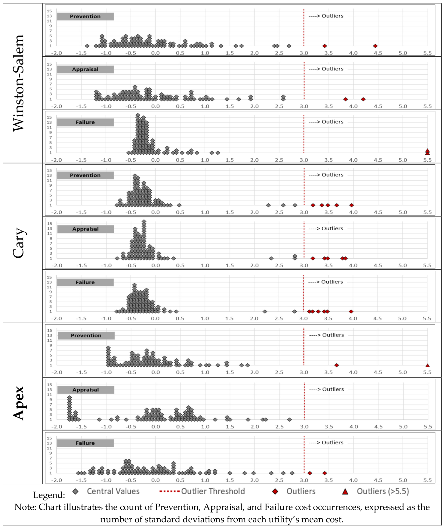
After the data for the water analysis was acquired and categorized, the data was analyzed for outliers. Outliers were defined as exceeding +/− 3 sample standard deviations away from the sample mean. For the study, 96 samples were obtained for prevention, appraisal, and failure categories, and their statistical summary for each municipality is shown in

Table 3. Water utility PAF outlier analysis.

Municipality	Values	Prevention	Appraisal	Failure
Winston-Salem	Mean =	$651,000	$290,000	$677,000
	Median =	$572,000	$250,000	$455,000
	Std Dev =	$290,000	$151,000	$937,000
	Outliers =	2	2	2
Cary	Mean =	$409,000	$321,000	$392,000
	Median =	$306,000	$221,000	$286,000
	Std Dev =	$369,000	$347,000	$375,000
	Outliers =	5	5	6
Apex	Mean =	$137,000	$31,000	$92,000
	Median =	$115,000	$32,000	$84,000
	Std Dev =	$131,000	$17,000	$54,000
	Outliers =	2	0	2

Notes: This table displays the sample mean and corresponding standard deviation for each dataset, as well as the count of outliers identified in each.

. Figure 1 graphically shows the results of the municipal PAF outlier analysis. Once the analyses were completed and the outliers identified, the outliers were removed from the remainder of the analysis.

2.8. Statistical General Model Analysis

Prevention, appraisal, failure, and opportunity costs are the categories analyzed in this study, representing the main variables and the data collected for analysis. The tests analyzed whether the water utilities in North Carolina have the same distribution as the ones in Texas. As described earlier, after the data were collected, a curve was fitted, using the R-squared value for goodness of fit, and the intersection of the curves for each of the prevention, appraisal, and failure categories was determined.

Table 4. Research hypotheses (water utilities).

Research Hypotheses (Water Utilities)
Null Hypotheses	Test Statistics	Test Statistic Variable Definitions
HypothesisW1: The relative NC Water Utility Total COQ costs are equal to the relative TX Water Utility Total COQ costs.	HW0a4-j: p4-j = p4-4 HW1a4-1: p4-1 ≠ p4-4 HW1a4-2: p4-2 ≠ p4-4 HW1a4-3: p4-3 ≠ p4-4	Pi-j represent a subset of the regression coefficients for the i and j variables i = The COQ Variables   = 1 (Prevention)   = 2 (Appraisal)   = 3 (Failure)   = 4 (Total COQ) j = The NC & TX Water Variables   = 1 (Winston-Salem)   = 2 (Cary)   = 3 (Apex)   = 4 (Texas Water Utilities)
HypothesisW2: The relative NC Water Utility Prevention quality costs are equal to the relative TX Water Utility Prevention quality costs.	HW0a1-j: p1-j = p1-4 HW1a1-1: p1-1 ≠ p1-4 HW1a1-2: p1-2 ≠ p1-4 HW1a1-3: p1-3 ≠ p1-4	Pi-j represent a subset of the regression coefficients for the i and j variables i = The COQ variables j = The NC & TX Water Variables
HypothesisW3: The relative NC Water Utility Appraisal quality costs are equal to the relative TX Water Utility Appraisal quality costs.	HW0a2-j: p2-j = p2-4 HW1a2-1: p2-1 ≠ p2-4 HW1a2-2: p2-2 ≠ p2-4 HW1a2-3: p2-3 ≠ p2-4	Pi-j represent a subset of the regression coefficients for the i and j variables i = The COQ Variables j = The NC & TX Water Variables
HypothesisW4: The relative NC Water Utility Failure quality costs are equal to the relative TX Water Utility Failure costs.	HW0a3-j: p3-j = p3-4 HW1a3-1: p3-1 ≠ p3-4 HW1a3-2: p3-2 ≠ p3-4 HW1a3-3: p3-3 ≠ p3-4	Pi-j represent a subset of the regression coefficients for the i and j variables i = The COQ Variables j = The NC & TX Water Variables
HypothesisW5: The Water Utility Opportunity Costs are not material, <0.5% of the total asset base.	HW0ci: WUOCi < 0.5% HW1ci: WUOCi ≥ 0.5%	WU = Water Utility BC = Opportunity Cost i = ith Water Utility

shows the testable hypotheses for the Potable Water Utility Infrastructure.

3. Results

3.1. Statistical Water Analysis—General Model and Data

The two-sample Kolmogorov–Smirnov (KS tests), evaluated in the mathematical-based program MATLAB (Version R2022b), was used to assess whether the two datasets were drawn from the same continuous distribution. The ks2stat value (also known as the Kolmogorov–Smirnov statistic) represents the maximum absolute difference between the cumulative distribution function of the two samples. A larger ks2stat value indicates a greater difference between the compared distributions, suggesting that they are likely from different populations. MATLAB will generate an h-value equal to “1” if the test rejects the null hypothesis at the 5% significance level, or equal to “0” otherwise. The p-value (or probability value) describes how likely it is that the data would have occurred by random chance (i.e., that the null hypothesis is true).

Table 5. KS test results for Texas municipalities’ COQ vs. NC municipalities’ COQ.

Set 1	Variable	Set 2	Variable	h	Result	p	ks2stat
Total COQ Texas Municipal Data Compared to Winston-Salem, Cary, and Apex
BWT	p4-4	WSWT	p4-1	1	Reject Null Hyp	1.1 × 10−4	0.3490
BWT	p4-4	CWT	p4-2	1	Reject Null Hyp	4.3 × 10−7	0.4375
BWT	p4-4	AWT	p4-3	1	Reject Null Hyp	1.1 × 10−2	0.2552
Prevention COQ Texas Municipal Data Compared to Winston-Salem, Cary, and Apex
BWP	p1-4	WSWP	p1-1	1	Reject Null Hyp	0.0471	0.2115
BWP	p1-4	CWP	p1-2	1	Reject Null Hyp	9.6 × 10−6	0.3822
BWP	p1-4	AWP	p1-3	1	Reject Null Hyp	8.4 × 10−3	0.2554
Appraisal COQ Texas Municipal Data Compared to Winston-Salem, Cary, and Apex
BWA	p2-4	WSWA	p2-1	0	Failed to Reject Null Hyp	0.1703	0.1700
BWA	p2-4	CWA	p2-2	1	Reject Null Hyp	8.0 × 10−6	0.3820
BWA	p2-4	AWA	p2-3	0	Failed to Reject Null Hyp	0.1383	0.1771
Failure COQ Texas Municipal Data Compared to Winston-Salem, Cary, and Apex
BWF	p3-4	WSWF	p3-1	1	Reject Null Hyp	2.1 × 10−6	0.4017
BWF	p3-4	CWF	p3-2	1	Reject Null Hyp	1.1 × 10−4	0.3386
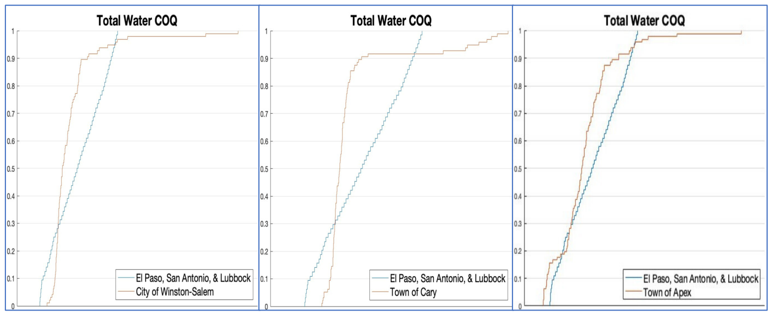
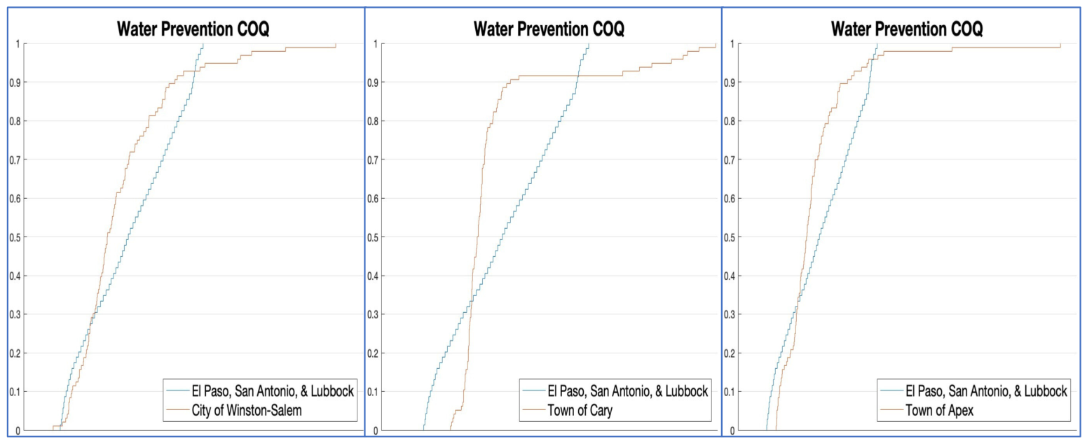
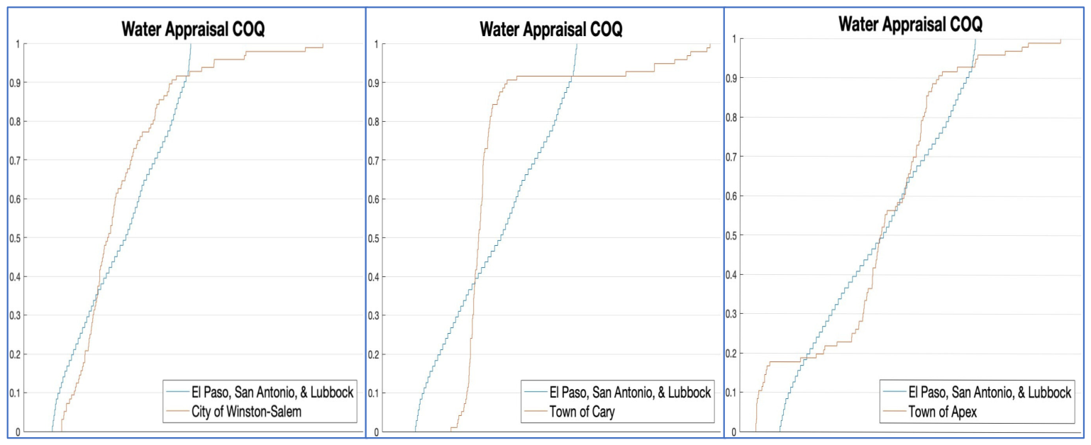
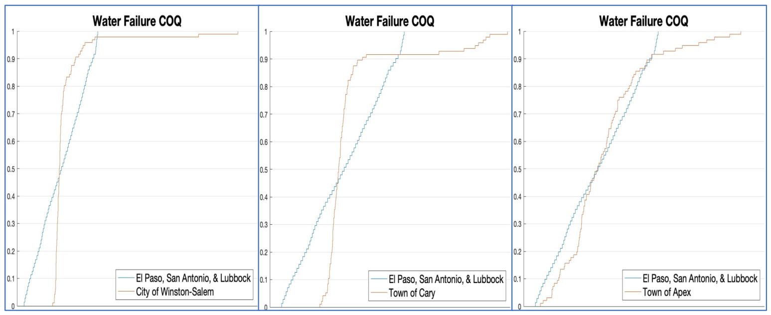
BWF	p3-4	AWF	p3-3	0	Failed to Reject Null Hyp	0.1792	0.1683

summarizes the results of the Kolmogorov–Smirnov tests, while Figure 2, Figure 3, Figure 4 and Figure 5 graphically present these outcomes. Three of the tests produced h-values equal to 0, indicating that the null hypothesis failed to be rejected at the 5% significance level (one for Winston-Salem and two for Apex). The figures illustrate how closely the data values align across the compared distributions.

Figure 2 corresponds to the KS test for the Total CoQ for this study, and Figure 3 corresponds to the Water Prevention CoQ sample. The smallest value of these KS stats is for the Water Prevention CoQ graph, and graphically, the deviation between the two samples is the least, as expected. All six plots of the above graphs represent a rejection of the null hypothesis.

Figure 4 corresponds to the KS test for the Appraisal CoQ for this study, and Figure 5 corresponds to the Water Failure CoQ sample. Of these six graphs, three represent samples that failed to reject the null hypothesis. These are the Winston-Salem Water Appraisal, the Apex Water Appraisal, and the Apex Water Failure samples. The representative graphs for the three that failed to reject the null hypothesis show the least deviation between the two analyzed samples.

3.2. Water Utility Material Analysis

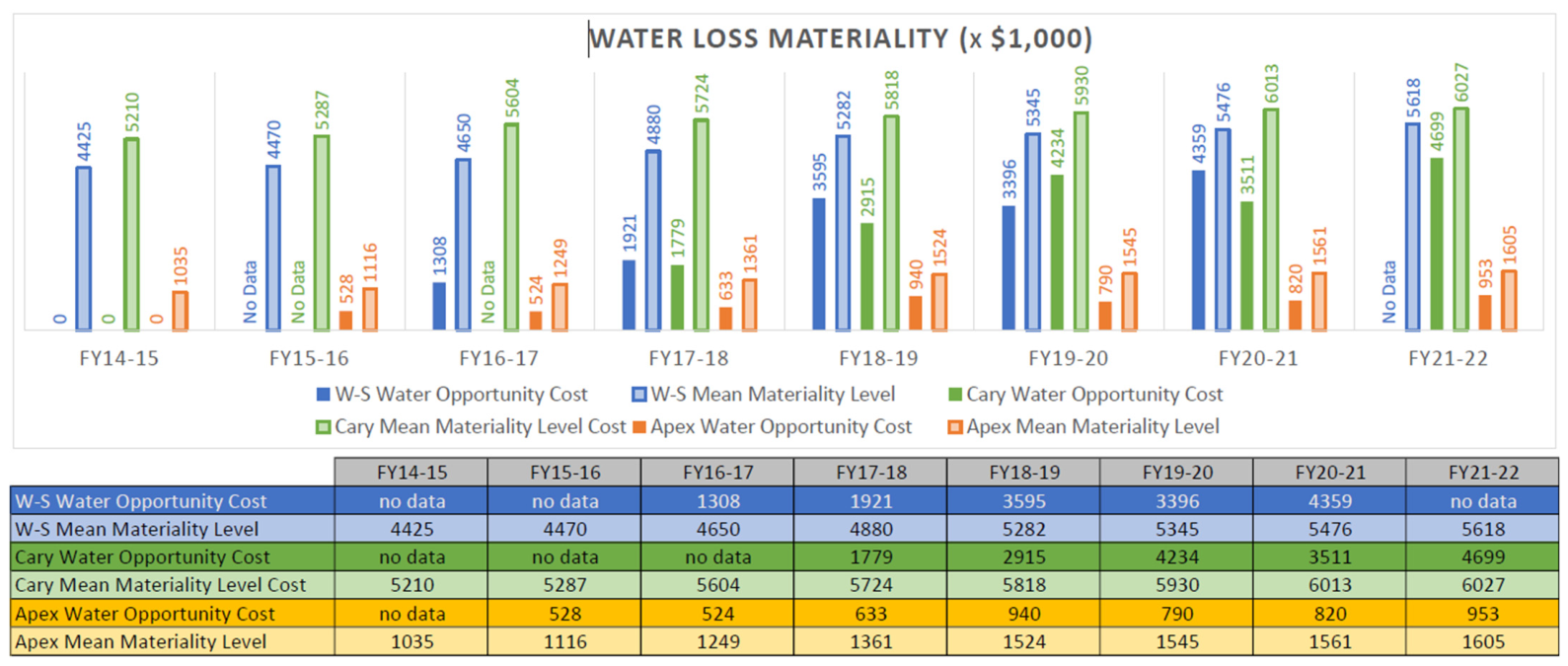
Consistent with the materiality approach established in the methodology, an expense of a system is deemed to be “material” if it is greater than 0.5% of the total assets of a company [11] (p. 155). Using this definition, asset information for the three municipalities was obtained along with water loss and water unit costs. For all three municipalities, the water and sanitary sewer assets were reported as one utility fund by the municipalities. Therefore, the water and sanitary sewer assets were used as the basis for determining materiality. Data was requested for eight consecutive years, and as Figure 6 shows, some data was not available and is shown as “no data” when this occurred. As Figure 6 shows, The Water Opportunity Cost for each municipality in the study was less than their respective Mean Materiality Level Cost. Therefore, the Water Opportunity Cost was not considered to be material in this study. It should be noted that the evaluation of opportunity cost in this study is based on an operational definition represented by water loss within the distribution system. Other potential components of opportunity costs, such as capital allocation, system capacity, or revenue-related impacts, were not included. In this context, this conclusion applies only within the scope of this definition.

For this study, opportunity cost is operationally defined as the economic value associated with water losses within the distribution system, based on measurable data available from participating municipalities. While the broader economic definition of opportunity cost includes alternative uses of resources such as deferred capital investments, system capacity allocation, and revenue impacts, these components were not directly quantifiable within the scope of this study. As a result, water loss was used as a practical and consistent proxy for opportunity cost across municipalities. Given that water loss represents a primary and measurable form of resource inefficiency in water utility systems, its use is considered sufficient for evaluating the relative materiality of opportunity costs in this context.

3.3. Analysis Results

The Texas study selected three municipalities representing different water source combinations and county water uses. During the time of the original study,

• San Antonio obtained 100% of its water from groundwater, with primarily urban use.
• Lubbock obtained approximately 24% of its water from groundwater, with primarily irrigation use.
• El Paso obtained approximately 66% of its water from groundwater, with water use split almost evenly between urban and irrigation.

Using the Hickory Municipal Classification System (Hickory MCS), San Antonio was classified as a Premier municipality, El Paso as an “A”-Class municipality, and Lubbock as a “C”-Class municipality. Four major variables were present in the Texas study: location (El Paso and San Antonio were ~550 miles apart), water sources, water usage, and population size. In contrast, the North Carolina study attempted to minimize variables by selecting an “A-Class,” “B-Class,” and “C-Class” municipality within ~90 miles, all using 100% surface water and with primarily urban/rural populations. These municipalities were chosen to eliminate some of the variables there were witnessed in the Texas study with population being the variable tested.

Table 6. Summary of hypothesis testing results for water utility CoQ categories.

Hypotheses (Water Utilities)
Null Hypotheses	Test Statistics	Test Statistic Variable
HypothesisW1: The relative NC Water Utility Total COQ costs are equal to the relative TX Water Utility Total COQ costs.	HW0a4-j: p4-j = p4-4 HW1a4-1: p4-1 ≠ p4-4 HW1a4-2: p4-2 ≠ p4-4 HW1a4-3: p4-3 ≠ p4-4	Smirnov Non-Parametric Test for Two Independent Samples Reject HW0a4-1: Kstat = 0.35 & h = 1 Reject HW0a4-2: Kstat = 0.44 & h = 1 Reject HW0a4-3: Kstat = 0.26 & h = 1
HypothesisW2: The relative NC Water Utility Prevention quality costs are equal to the relative TX Water Utility % Prevention quality costs.	HW0a1-j: p1-j = p1-4 HW1a1-1: p1-1 ≠ p1-4 HW1a1-2: p1-2 ≠ p1-4 HW1a1-3: p1-3 ≠ p1-4	Smirnov Non-Parametric Test for Two Independent Samples Reject HW1a1-1: Kstat = 0.21 & h = 1 Reject HW1a1-2: Kstat = 0.38 & h = 1 Reject HW1a1-3: Kstat = 0.26 & h = 1
HypothesisW3: The relative NC Water Utility Appraisal quality costs are equal to the relative TX Water Utility Appraisal quality costs.	HW0a2-j: p2-j = p2-4 HW1a2-1: p2-1 ≠ p2-4 HW1a2-2: p2-2 ≠ p2-4 HW1a2-3: p2-3 ≠ p2-4	Smirnov Non-Parametric Test for Two Independent Samples Failed to Reject HW1a2-1: Kstat = 0.17 & h = 0 Reject HW1a2-2: Kstat = 0.38 & h = 1 Failed to Reject HW1a2-3: Kstat = 0.18 & h = 0
HypothesisW4: The relative NC Water Utility Failure quality costs are equal to the relative TX Water Utility Failure costs.	HW0a3-j: p3-j = p3-4 HW1a3-1: p3-1 ≠ p3-4 HW1a3-2: p3-2 ≠ p3-4 HW1a3-3: p3-3 ≠ p3-4	Smirnov Non-Parametric Test for Two Independent Samples Reject HW1a3-1: Kstat = 0.40 & h = 1 Reject HW1a3-2: Kstat = 0.34 & h = 1 Failed to Reject HW1a3-3: Kstat = 0.17 & h = 0
HypothesisW5: The Water Utility Opportunity Costs are not material, <0.5% of the total asset base.	HW0ci: WUOCi < 0.5% HW1ci: WUOCi ≥ 0.5%	Graphical analysis summarized in Figure 6 shows that Water Utility Opportunity Costs for all three municipalities are not material.

summarizes the results of five hypotheses regarding Total CoQ, prevention, appraisal, failure, and opportunity costs. Four of the hypotheses were tested using the Kolmogorov–Smirnov (KS) test for two independent samples:

• Hypothesis W1 (Total CoQ costs): All three North Carolina municipalities rejected the null hypothesis, indicating that Total CoQ costs were not consistent with Texas municipalities.
• Hypothesis W2 (prevention costs): All three North Carolina municipalities rejected the null hypothesis. Cary (B-Class) deviated more than Winston-Salem (A-Class) and Apex (C-Class).
• Hypothesis W3 (appraisal costs): Winston-Salem and Apex failed to reject the null hypothesis, indicating consistency with Texas municipalities.
• Hypothesis W4 (failure costs): Apex failed to reject the null hypothesis, while Winston-Salem and Cary rejected it.

Two-thirds of the components of Total CoQ’s null hypotheses were rejected, which aligns with the rejection of the Total CoQ hypothesis itself. Hypothesis W6 on opportunity costs, assessed via graphical analysis, showed that the costs for all three municipalities were not material (<0.5% of total asset base).

Several factors may contribute to the rejected null hypotheses. While the North Carolina municipalities were selected to minimize variation in geography, water source, and operational structure, the Texas municipalities exhibited greater diversity in these variables. As a result, differences in CoQ between the two groups may reflect not only population size and classification effects, but also environmental, operational, and accounting variations between the systems:

• Municipal variables: Texas municipalities differed in location, water use patterns, water sources, and population, while North Carolina municipalities were more uniform. These differences may influence system scale, complexity, and demand characteristics, which in turn affect how prevention, appraisal, and failure costs are distributed.
• Environmental differences: North Carolina and Texas have differing rainfall patterns, soil conditions, temperature variations, and drought exposure. These factors can affect infrastructure stress, leakage rates, and maintenance frequency, thereby influencing both prevention and failure costs.
• Accounting differences: Variations in how costs are defined, tracked, and categorized within the study framework, which relied on municipal records and was then reviewed with municipal staff for validation, may affect the allocation of expenses into PAF categories, introducing differences in reported CoQ components independent of operational performance.
• Operational differences: Differences in technology adoption, regulatory requirements, maintenance strategies, and system management practices may influence cost structures across municipalities, particularly in the balance between prevention and appraisal activities.

Accordingly, the CoQ differences observed between North Carolina and Texas utilities should be interpreted as indicative of system-level variation rather than attributable to any single factor.

4. Discussions, Conclusions and Future Research

4.1. Discussion and Conclusions

This study broadens the understanding of municipal water utility Cost of Quality (CoQ) by comparing municipalities in North Carolina and Texas. The analysis revealed significant differences in Total CoQ costs between the two states, largely attributable to variations in environmental conditions, operational practices, and accounting differences (including categorization and record-keeping practices). For example, North Carolina municipalities often operate under different regulatory and climatic conditions than those in Texas, which can influence resource allocation and cost structures. At the component level, prevention costs showed consistent differences across municipalities, suggesting that proactive measures such as infrastructure maintenance and water quality monitoring vary significantly by region. In contrast, appraisal and failure costs exhibited mixed patterns indicating that some municipalities prioritize quality assurance differently or experience varying levels of system failures.

These variations are likely driven by a combination of technological adoption, political priorities, and management practices within each municipality. Additionally, the Water Opportunity Cost was found to be immaterial for the municipalities in this study, meaning that its impact on overall CoQ was negligible. Collectively, these findings underscore the complexity of municipal water utility operations and highlight the importance of considering multiple variables, including environmental, operational, and accounting factors, when comparing CoQ across regions. Understanding these dynamics is critical for policymakers and utility managers seeking to optimize quality-related expenditures and improve service delivery in diverse geographic and regulatory contexts.

While this study does not directly address cost recovery or rate-setting practices, the CoQ framework provides information that may support water pricing decisions. By identifying the distribution of prevention, appraisal, and failure costs, utilities can better understand the financial implications of infrastructure performance and maintenance strategies, which are relevant to long-term cost recovery.

From a practical standpoint, the findings of this study provide several actionable insights for municipal water utilities seeking to improve service quality while managing costs. Utilities may benefit from increasing investment in prevention activities, such as proactive infrastructure maintenance and water quality monitoring, as these were consistently associated with differences in overall CoQ. Additionally, improving cost tracking and categorization practices can provide better visibility into quality-related expenditures, enabling more informed decision-making. Utilities may also evaluate the balance between prevention, appraisal, and failure costs to identify inefficiencies, particularly in systems where higher failure costs suggest underinvestment in preventative measures. Finally, benchmarking against similarly classified municipalities using frameworks such as the HMCS may help utilities identify performance gaps and prioritize targeted improvements.

Beyond the statistical methods applied in this study, additional insight may be gained through the use of machine learning (ML) approaches, which can help identify relationships among Cost-of-Quality components that are not easily observed using the methods applied here. These approaches could be used to group municipalities based on similarities in their Cost-of-Quality profiles without relying on population or another predefined classification system such as the Hickory MCS and may also provide a clearer understanding of which factors most strongly influence prevention, appraisal, and failure costs across different utility systems.

In addition, applying machine learning techniques to the time-based structure of the dataset may help identify periods of unusual cost behavior, which could indicate operational inefficiencies or emerging infrastructure issues. These variations may be associated with real-world changes such as shifts in management practices, changes in maintenance strategies, equipment upgrades or failures, and the gradual degradation of infrastructure systems requiring increased repair effort. External conditions may also influence these patterns, including changes in customer base, regulatory requirements, or broader events such as the operational impacts observed during the COVID-19 period. Such approaches, as demonstrated in recent studies, allow for a more detailed examination of how cost elements relate to one another and may provide additional insight beyond the statistical techniques used in this study. This perspective aligns with recent work demonstrating that machine learning enables a shift from traditional, manually driven analysis (such as that performed in this study) toward a more efficient data-driven approach that can identify relationships within complex datasets and significantly reduce the effort required for large-scale analysis [20].

It should also be noted that a substantial portion of the effort in this study involved the manual collection, organization, and standardization of cost data across multiple municipalities. Differences in accounting structures, terminology, and reporting formats required significant effort to categorize costs into consistent PAF classifications and align them with a common format prior to performing the statistical analysis. In this context, machine learning methods may reduce manual processing and improve consistency in how data are classified and compared. These methods may also help identify similarities in cost categories and make datasets easier to organize and analyze. This could make similar studies more efficient and easier to expand across multiple systems.

4.2. Future Research

Potential future research for this study can be categorized into three areas: geography, infrastructure, and population. First, future research could include municipalities from other regions of North Carolina, such as the mountain and coastal areas, to capture the impact of geographic and environmental differences on Cost of Quality. The municipalities in this study were chosen from Central North Carolina to minimize this geographic impact. Second, future research could also include a broader range of municipalities, which would allow for comparisons across varying population sizes and classifications beyond the single Class A, Class B, and Class C municipalities that were selected and included in this study. Finally, future research can expand the work done here to include other infrastructure, such as wastewater systems, roads, and electrical networks, to name a few. Studying additional infrastructure would provide a more comprehensive understanding of how quality-related costs differ across public services. These three steps would help identify patterns and operational differences that were not fully explored in this study, offering a stronger foundation for improving municipal management practices. Ultimately, this expanded research could support policymakers and public managers in making more informed decisions about resource allocation, cost control, and service quality improvements. Future research may explore the integration of CoQ metrics into water utility rate-setting frameworks to better align operational performance with sustainable cost recovery and long-term financial planning.

In addition, future research may incorporate machine learning and data-driven methodologies to analyze Cost-of-Quality datasets in a more structured and efficient manner, as demonstrated in recent studies [20] utilizing intelligent analytical approaches. The development of a repeatable process for applying these methods to municipal cost data would be particularly valuable, as it would significantly reduce the level of manual effort required for data collection, categorization, and standardization. Such a process would allow for a much faster expansion of similar studies across larger datasets, additional municipalities, and longer time periods.

Establishing this capability would also support expansion into other infrastructure systems, allowing Cost-of-Quality analysis to be applied more broadly across domestic water, wastewater, stormwater, transportation, and other public service infrastructure systems. While the implementation of such methods is beyond the scope of the current study, their potential to accelerate and scale future research makes them a highly valuable area for continued development.

References

1. Juran Joseph, M.; De Feo Joseph, A. Juran’s Quality Handbook: The Complete Guide to Performance Excellence, 6th ed.; McGraw-Hill: New York, NY, USA, 2010. [Google Scholar]
2. Juran, J.M. Quality-Control Handbook, 1st ed.; McGraw-Hill: New York, NY, USA, 1951. [Google Scholar]
3. Carr, L.P. Applying Cost of Quality to a Service Business. Sloan Manag. Rev. 1992, 33, 72–77. [Google Scholar]
4. Banasik, M.A.; Beruvides, M.G. A Case Study of the Costs of Quality: Water Utilities. Eng. Manag. J. 2012, 24, 3–14. [Google Scholar] [CrossRef] [Scilit]
5. Arrandale, T. What’s the Value of Water? Drought-Plagued Regions Struggle to Conserve Water and Make Money. In Governing the States and Localities; CQ Press: Washington, DC, USA, 2014. Available online: http://www.governing.com/topics/transportation-infrastructure/gov-drought-water-revenue.html (accessed on 6 July 2015).
6. Dalesio, E.P.N.C. Senate moves to take airport from Charlotte. Washington Examiner, 12 March 2013. Available online: https://www.travelerstoday.com/articles/5318/20130314/north-carolina-senate-tries-force-states-takeover-charlotte-douglas-international.htm (accessed on 3 July 2015).
7. Leslie, L. House Votes to Take Asheville’s Water System. 11 April 2013. Available online: http://www.wral.com/house-votes-to-take-asheville-s-water-system-/12332379/ (accessed on 3 July 2015).
8. Texas State Highway 130. Available online: https://en.wikipedia.org/wiki/Texas_State_Highway_130 (accessed on 3 July 2015).
9. NCGS. North Carolina General Statutes, Chapter 62: Public Utilities (160A-411). Available online: https://www.ncleg.gov/EnactedLegislation/Statutes/HTML/ByChapter/Chapter_160A.html (accessed on 10 September 2016).
10. Feigenbaum, A.V. Total Quality Control. Harv. Bus. Rev. 1956, 34, 93–101. [Google Scholar]
11. Banasik, M.A. A Study of the Costs of Quality in a Renewable Resource Environment. Doctoral Dissertation, Texas Tech University, Lubbock, TX, USA, 2009. [Google Scholar]
12. Wagner, S.F. Introduction to Statistics; Harper Perennial: New York, NY, USA, 1992. [Google Scholar]
13. Nelson, K.; Stenberg, C. Managing Local Government: An Essential Guide for Municipal and County Manager; CQ Press: Washington, DC, USA, 2018. [Google Scholar]
14. ANSI/ASQC Q94; Quality Management and Quality System Elements—Guidelines. American Society for Quality Control: Milwaukee, WI, USA, 1987.
15. BS 6143-1; Guide to the Economics of Quality—Part 1: Process Cost Model. British Standards Institute: London, UK, 1992.
16. BS 6143-2; Guide to the Economics of Quality—Part 2: Prevention, Appraisal and Failure Model. British Standards Institute: London, UK, 1990.
17. ISO 9004; Managing for the Sustained Success of an Organization—A Quality Management Approach. International Standards Organization: Geneva, Switzerland, 2009.
18. Harrington, H.J. Poor-Quality Cost; ASQC Quality Press: Milwaukee, WI, USA, 1987. [Google Scholar]
19. Feigenbaum, A.V. Total Quality Control: Engineering and Management; McGraw-Hill: New York, NY, USA, 1961. [Google Scholar]
20. Wang, H.; Cao, H.; Yang, L. Machine Learning-Driven Multidomain Nanomaterial Design: From Bibliometric Analysis to Applications. ACS Appl. Nano Mater. 2024, 7, 26579–26600. [Google Scholar] [CrossRef] [Scilit]
21. Asher, J.M. Cost of Quality in Service Industries. Int. J. Qual. Reliab. 1988, 5, 38–46. [Google Scholar] [CrossRef] [Scilit]
22. Juran, J.M.; Gyrna, F.M. Quality Planning and Analysis, 3rd ed.; McGraw-Hill, Inc.: New York, NY, USA, 1993. [Google Scholar]
23. Pyzdek, T.; Keller, P. The Six Sigma Handbook, 4th ed.; McGraw-Hill Education (India) Private Limited: New Delhi, India, 2014. [Google Scholar]
24. Mitchell, T.M. Machine Learning; McGraw-Hill: New York, NY, USA, 1997. [Google Scholar]
25. Senge, P.M. The Fifth Discipline: The Art & Practice of the Learning Organization; Doubleday: New York, NY, USA, 2006. [Google Scholar]
26. Revell, C.S.; Whitlatch, E.E.; Wright, J.R. Civil And Environmental Systems Engineering; Prentice Hall: Hoboken, NJ, USA, 1997. [Google Scholar]
27. Barker, J.A. Paradigms: The Business of Discovering the Future; HarperBusiness: New York, NY, USA, 1992. [Google Scholar]
Figure 1. Municipal PAF outlier analysis.
Water 18 01573 g001
Figure 2. Water Total COQ cumulative distribution function (CDF).
Water 18 01573 g002
Figure 3. Water Prevention CoQ cumulative distribution function (CDF).
Water 18 01573 g003
Figure 4. Water Appraisal CoQ cumulative distribution function (CDF).
Water 18 01573 g004
Figure 5. Water Failure CoQ cumulative distribution function (CDF).
Water 18 01573 g005
Figure 6. Water loss materiality (Winston-Salem, Cary, and Apex). Note: Water Opportunity Costs remain below the established 0.5% materiality threshold for all municipalities.
Water 18 01573 g006