Morphometric and Multivariate Analysis of Geomorphological and Multi-Hazard Dynamics in the La Sabana River Basin, Acapulco–Mexico

Abstract

Coastal basins are systems highly susceptible to flooding and erosion, processes that intensify during extreme cyclonic events. This study aims to develop an integrated physical–geographic framework to characterize the geomorphological and multi-hazard dynamics of the La Sabana River basin in Acapulco, Guerrero, in southeastern Mexico. The methodology integrates the analysis of natural and anthropogenic landscape components, 19 morphometric indicators, and Principal Component Analysis (PCA) at the sub-basin scale. The results reveal a high drainage network density (3.8–5.4 km/km²) and short concentration times (0.98–2.75 h), indicating a rapid hydrological response and high susceptibility to flash floods and active erosion. Six critical sub-basins with concentration times ≤ 1.5 h have been identified, spatially coinciding with areas of high anthropogenic exposure. The hypsometric index values (0.04–0.388) indicate advanced geomorphological evolution in most sub-basins. Principal component analysis (PCA) explained 65.8% of the total variance in the first two components: component 1 (52.7%) is linked to basin size and drainage network organization, and component 2 (13.1%) is associated with basin shape. The findings of this research have provided a spatially explicit, robust, and replicable framework that helps strengthen risk governance and guide land-use planning in tropical coastal basins exposed to hydrometeorological hazards.

1. Introduction

Coastal zones are among the most dynamic and hazardous territorial contexts on the planet due to the continuous interaction of oceanic, atmospheric, geological, and biological processes at the Earth’s edge [1,2]. These transitional systems concentrate dense human populations, critical infrastructure, and high-value economic activities, making them particularly exposed to multiple threats triggered by hydrometeorological events [3,4]. In tropical regions, the recurrence of cyclones, heavy rainfall, and extreme events significantly increases the frequency and severity of floods and erosion, generating increasingly complex, interconnected multi-hazard risk scenarios [5].

This situation is exacerbated by unplanned urban expansion, for example, through the occupation of floodplains and unstable slopes, as well as the transformation of natural systems that regulate hydrological and geomorphological behavior [6,7]. Global evidence confirms that human settlements have expanded rapidly into flood-prone areas in coastal regions since the 1950s; this trend substantially increases communities’ exposure to hydrometeorological hazards [8].

In this context, coastal risk governance has emerged as a central axis for territorial planning and sustainable development, requiring integrated approaches that link scientific knowledge with decision-making [9,10]. However, the physical–geographical knowledge of coastal systems is still only partially incorporated into operational risk governance instruments. Although geomorphological and hydrological studies of coastal basins have advanced significantly, their integration into territorial planning and adaptive risk management frameworks remains insufficient [11,12].

Moving in this direction requires tools that can translate physiographic knowledge of the territory into useful information for decision-making. In this context, morphometric analysis of watersheds has become an effective approach to describe relief organization, drainage structure, and hydrological response to extreme events [13,14]. Morphometric indicators enable the quantitative characterization of watershed hydrological behavior and the assessment of their susceptibility to hazards such as floods and erosion [15,16]. Their effectiveness has been widely supported across diverse physiographic contexts, thereby consolidating them as reference tools for the spatial assessment of hydrogeomorphological risk [17,18].

Morphometric analysis has been widely applied in diverse physiographic and climatic contexts, demonstrating its effectiveness as a transferable tool for flood risk assessment. In South Asia, studies of river basins in India and the Himalayan region have shown that parameters such as drainage density, bifurcation ratio, and elongation ratio characterize hydrological behavior and susceptibility to erosion, and guide prioritization strategies for flood mitigation [19,20,21,22]. In Southeast Asia, its combination with hydrological models has identified sub-basins susceptible to flash floods in tropical basins of Nepal and Thailand, confirming that high drainage density, low elongation ratios, and short concentration times are consistent indicators of rapid hydrological response [23,24]. In the Middle East and Europe, studies in arid wadi systems in Saudi Arabia and mountain basins in southern Italy have validated the correspondence between morphometric indicators and documented risk events, even in data-scarce environments [25,26,27]. In Latin America, a recent study in the Mantaro basin, Peru, identified that 74% of the area has high to very high susceptibility to flooding, with steep slopes and dense drainage networks as dominant factors [28]. However, integrated frameworks that combine morphometric analysis, multivariate techniques, and physical–geographic characterization in tropical coastal basins exposed to extreme cyclonic events remain scarce, a gap that the present study seeks to address.

The integration of these indicators using multivariate techniques, such as principal component analysis (PCA), enables the objective identification of the dominant controls that structure the hydrogeomorphological dynamics of watersheds [29]. Implementing this approach allows for the reduction in highly correlated morphometric variables into interpretable components associated with drainage density, relief, and basin shape [17]. However, there remains a growing need to develop integrated frameworks that link physical–geographic analysis to multi-hazard risk assessment and management, particularly in tropical basins, where interactions between natural processes and anthropogenic dynamics create complex scenarios of exposure and vulnerability [30,31].

The La Sabana River basin, located in the southern Pacific coastal region of Mexico, represents an emblematic case of this problem. Land-use changes associated with urban growth have been identified as primary drivers of increased flood risk in Mexican coastal basins, reducing infiltration capacity and accelerating surface runoff, even under stable precipitation regimes [7].

This dynamic is particularly visible in Acapulco, a municipality that has repeatedly faced extreme hydrometeorological events, the severity of which has been amplified by extreme rainfall, urbanization in high-risk areas, and environmental degradation. Events such as Hurricane Paulina (1997), Tropical Storm Manuel (2013), Hurricane Otis (2023), the most intense recorded in the Mexican Pacific, and Hurricane John (2024) have highlighted the region’s vulnerabilities to such phenomena.

Studies of these events have documented severe failures in early warning systems, crisis coordination, and risk communication [22,23], as well as extensive erosion, flooding, and infrastructure damage in the basin’s tourist and residential areas [32]. These findings highlight the limitations of existing risk governance frameworks, demonstrating persistent shortcomings in understanding the territory and considering the basin’s physical–geographic conditions in risk management and preventive planning processes.

Given this scenario, the present study aims to develop an integrated physical–geographic framework to strengthen multi-hazard risk governance associated with tropical storms in coastal basins. For this purpose, it combines the analysis of natural and anthropogenic landscape components, hydrogeomorphological and morphometric characterization, and multivariate techniques. Within this framework, multi-hazard dynamics are approached from a geomorphological perspective, emphasizing the interaction between hydrological processes, such as runoff generation and flood propagation, and slope processes, particularly landslides, under extreme rainfall conditions. Rather than modeling each hazard independently, the study identifies the spatial configuration of basin attributes that jointly enhance susceptibility to coupled hydrogeomorphological responses. This approach makes it possible to identify the dominant controls on hazardous geomorphological dynamics and to support spatially explicit territorial intervention decisions in the La Sabana River basin, southern Mexico.

2. Materials and Methods

2.1. Study Area

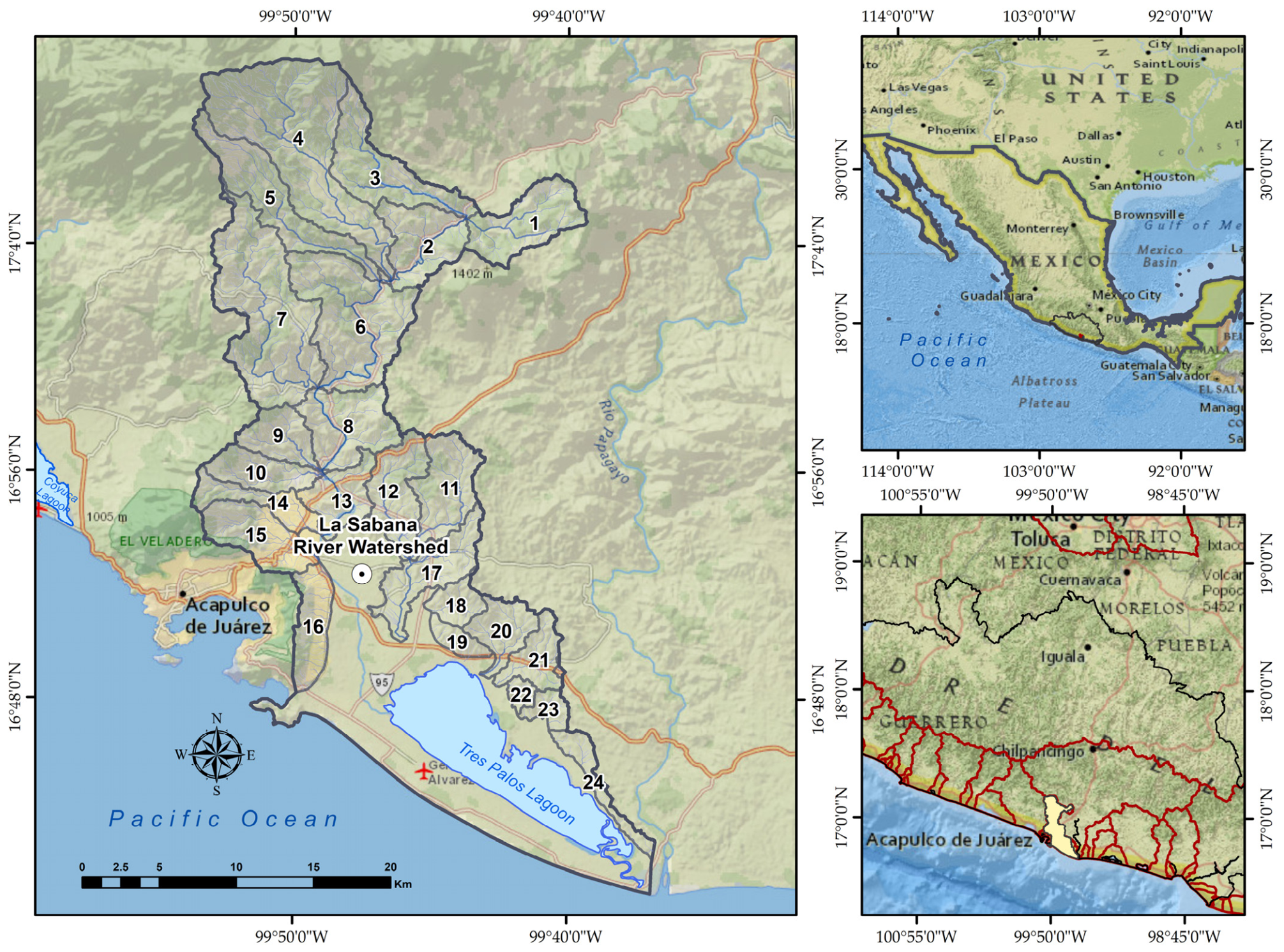
The La Sabana River basin is in southwestern Mexico, specifically in southern Guerrero. It is delimited by the coordinates 16°42′17″ north latitude and −99°54′37″ west longitude, with an area of 740.14 km². The basin’s surface area is located primarily within the municipality of Acapulco de Juárez (94.99%), while the western portion encompasses 5.01% of the territory of the municipality of Coyuca de Benítez. It is an exorheic basin, as the main river flows into the Tres Palos Lagoon, which in turn empties into the Pacific Ocean (Figure 1).

2.2. Methodology

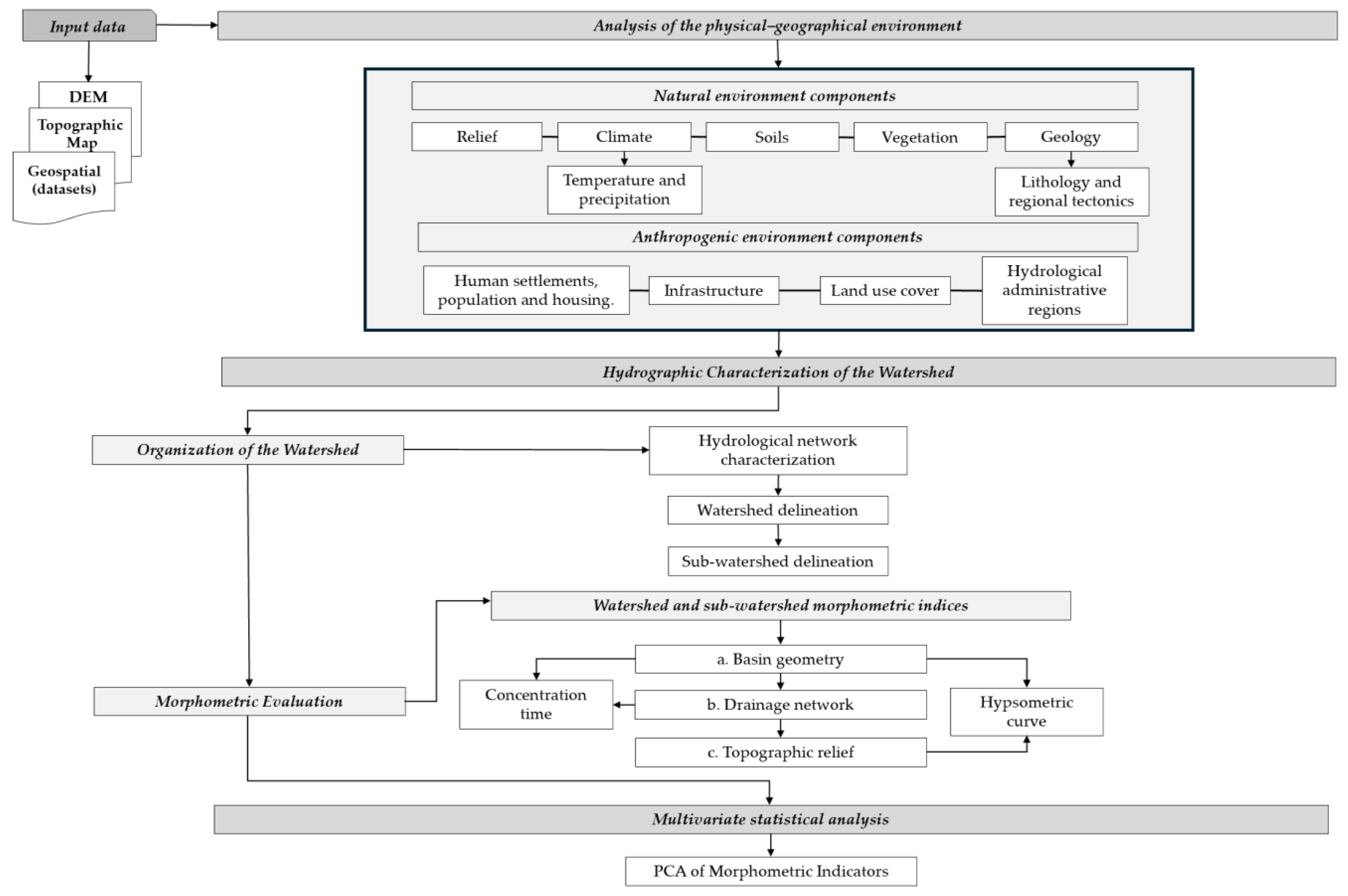
The research design follows a sequential order in three stages. The first stage focuses on describing the basin’s physical–geographic environment, including its natural and anthropogenic components. The second stage involves a physiographic characterization of the watershed and the La Sabana River subsystems using morphometric indicators. The final stage is a statistical analysis using principal component analysis (PCA) to integrate the morphometric indicators used in this study. Figure 2 illustrates the methodological sequence used in the study, and it is explained in detail in the following sections.

A generative AI tool was used solely to provide writing suggestions and English grammar corrections. No AI was used for data analysis, interpretation of results, or generation of scientific content.

2.3. Data

The data in this research comes from official geographic sources for Mexico. The physical–geographic analysis was performed using topographic maps in vector format at a scale of 1:50,000 and also with raster data from the DEM corresponding to the Mexican Elevation Continuum 3.0 of the National Institute of Statistics and Geography, with a spatial resolution of 15 m [33]. Spatial processing was performed using the WGS 84/UTM Zone 14 N (EPSG:32614) coordinate reference system. Morphometric indicators were calculated and mapped using QGIS 3.44. The R programming (version 4.5.1) was used for supplementary statistical analyses and for generating graphics using the FactoMineR package (version 2.14).

2.4. Analysis of the Physical–Geographical Environment

The physical–geographic analysis of the La Sabana River basin in this study is based on an integrated vision of the territory, in which the interplay between natural processes and anthropogenic dynamics is conceived from a perspective on the society-nature relationship that influences the functioning of a fluvial system [34,35,36].

From a natural perspective, the physical conditions that define the complex interactions among tectonic, climatic, and erosive processes shaping the basin’s geomorphological and hydrological dynamics are interpreted [37]. The role of relief energy as a conditioning factor in natural processes is highlighted [38,39,40].

The climatic regime is considered a triggering factor that conditions the basin’s hydrological response through its hydrometeorological framework, determined by precipitation and temperature [41,42]. Soil and vegetation development act as an interface in the climate-relief relationship, influencing infiltration, surface runoff, and terrain stability [35,36,37], while regional lithology and tectonics exert structural controls that shape and influence the evolution of the fluvial system [43,44].

Complementarily, anthropogenic activity has acquired an important role as a forcing factor in the physical–geographic system, interfering with the modification of natural channels, increasing soil impermeability, and altering hydrological connectivity through the expansion of human settlements, infrastructure development, and land-use changes [45]. In this sense, this study explains the anthropic components based on human settlements, population and housing, road infrastructure, and land use in the basin, and they are understood as factors that significantly modify the geomorphological and hydrological functioning, by transforming the natural conditions of the territory and favoring the configuration of spaces potentially exposed to the occurrence of dangerous geomorphological processes.

2.5. Hydrographic Characterization of the Watershed

This section presents the methodological approach used to characterize the physiographic elements of the La Sabana River hydrographic system and is structured in two stages. The first part focuses on characterizing the drainage network to differentiate the natural boundaries of the river system at the basin and sub-basin levels, followed by a morphometric evaluation at the sub-basin level. The methodological development combined geomorphological criteria and geospatial tools for each stage.

2.5.1. Spatial Organization of the Basin

In watershed studies, hydrographic delineation is the initial step, as it allows identification of the catchment area and the morphological elements that constitute it. In this stage, two criteria were used to differentiate the hydrographic system. First, topographic data at a 1:50,000 scale were derived from analogy maps, providing a preliminary characterization of the drainage network. This was followed by automated hydrological processing in GIS. The integration of both techniques enabled the inclusion of the geomorphological criterion as a control basis during automated processing, ensuring a coherent cartographic base for delineating the boundaries of the river system at the watershed and sub-watershed levels.

2.5.2. Morphometric Evaluation

Morphometric analysis in geomorphology studies the quantitative characteristics of topographic relief [46,47]. In the context of watersheds, evaluating morphometric indicators helps us understand the complexity of the relief through spatial patterns, thereby revealing its hydrogeomorphological dynamics [38,48,49,50,51]. For this study, the morphometric indicators were selected from the literature review by Shekar [52], who compiled 32 morphometric indices documented in the scientific literature. Of these, 19 indicators were selected, discarding those that produced redundant information. These indicators were grouped into three categories: (a) Watershed geometry, (b) Drainage network, and (c) Topographic relief (Table 1, Table 2 and Table 3). The process of extracting these values was developed in GIS, and they were calculated using the mathematical equation for each indicator, based on the DEM and the polygons that define the basin and sub-basin surfaces.

(a)

Basin Geometry

The morphometric indicators associated with basin geometry provided important information for understanding the hydrological and dynamic processes occurring within them [53,54].

Table 1. Morphometric indicators are associated with basin geometry and their mathematical expressions.

No.	Indicator	Symbol	Equation	Reference
1	Area (km2)	A	Basin polygon	[53]
2	Perimeter (km)	P	Catchment boundary	[53]
3	Maximum basin length (km)	Lb	Basin polygon	[55]
4	Maximum basin width (km)	Wb	Basin polygon	[55]
5	Elongation ratio	Re	$\mathrm{Re}=2 \sqrt{(\mathrm{A}/\mathrm{\pi })/\mathrm{L}\mathrm{b}}$	[53]
6	Form Factor	Ff	${\mathrm{F}}_{\mathrm{f}}=\mathrm{A}∕{\mathrm{L}\mathrm{b}}^2$	[56]

Table 1. Morphometric indicators are associated with basin geometry and their mathematical expressions.

No.	Indicator	Symbol	Equation	Reference
1	Area (km2)	A	Basin polygon	[53]
2	Perimeter (km)	P	Catchment boundary	[53]
3	Maximum basin length (km)	Lb	Basin polygon	[55]
4	Maximum basin width (km)	Wb	Basin polygon	[55]
5	Elongation ratio	Re	$\mathrm{Re}=2 \sqrt{(\mathrm{A}/\mathrm{\pi })/\mathrm{L}\mathrm{b}}$	[53]
6	Form Factor	Ff	${\mathrm{F}}_{\mathrm{f}}=\mathrm{A}∕{\mathrm{L}\mathrm{b}}^2$	[56]

(b)

Drainage network

The indicators associated with the drainage network enabled the description of hydrological connectivity and the efficiency with which runoff is channeled into the river system (Table 2). Their analysis proves to be an excellent indicator for recognizing drainage patterns influenced by structural control [57]. They have also been used to predict geomorphological dynamics, such as flooding, and to estimate erosion rates [15,58]. Studies have confirmed that the hierarchical structure of the drainage network reflects the interaction between lithological composition and sites susceptible to precipitation-triggered erosional dynamics [20,59].

Table 2. Morphometric indicators of the drainage network and their mathematical expressions.

No.	Indicator	Symbol	Equation	Reference
7	Stream order	U	Hierarchical rank	[38]
8	Number of streams	Nu	${\mathrm{N}}_{\mathrm{u}}={\mathrm{N}}_1+{\mathrm{N}}_2+{\mathrm{N}}_{\mathrm{n}}$	[38]
9	Total stream length	Tsl	Total length of streams	[48]
10	Main channel length	Lu	Distance from the channel head to the outlet	[48]
11	Bifurcation ratio	Rb	${\mathrm{R}}_{\mathrm{b}}={\mathrm{N}}_{\mathrm{u}}/{\mathrm{N}}_{\mathrm{u}+1}$	[53]
12	Stream frequency	Fs	${\mathrm{F}}_{\mathrm{s}}={\mathrm{T}}_{\mathrm{s}\mathrm{l}}∕\mathrm{A}$	[48]
13	Drainage texture	Dt	Dt = Nu/P	[48]
14	Drainage density	Dd	$\mathrm{D}\mathrm{d}={\displaystyle \frac{\mathrm{\Sigma }\mathrm{T}\mathrm{l}\mathrm{s}}{\mathrm{A}}}$	[48]

Table 2. Morphometric indicators of the drainage network and their mathematical expressions.

No.	Indicator	Symbol	Equation	Reference
7	Stream order	U	Hierarchical rank	[38]
8	Number of streams	Nu	${\mathrm{N}}_{\mathrm{u}}={\mathrm{N}}_1+{\mathrm{N}}_2+{\mathrm{N}}_{\mathrm{n}}$	[38]
9	Total stream length	Tsl	Total length of streams	[48]
10	Main channel length	Lu	Distance from the channel head to the outlet	[48]
11	Bifurcation ratio	Rb	${\mathrm{R}}_{\mathrm{b}}={\mathrm{N}}_{\mathrm{u}}/{\mathrm{N}}_{\mathrm{u}+1}$	[53]
12	Stream frequency	Fs	${\mathrm{F}}_{\mathrm{s}}={\mathrm{T}}_{\mathrm{s}\mathrm{l}}∕\mathrm{A}$	[48]
13	Drainage texture	Dt	Dt = Nu/P	[48]
14	Drainage density	Dd	$\mathrm{D}\mathrm{d}={\displaystyle \frac{\mathrm{\Sigma }\mathrm{T}\mathrm{l}\mathrm{s}}{\mathrm{A}}}$	[48]

(c)

Topographic Relief

Relief parameters, derived from the relationship among area, height, and relief, were essential for assessing the degree of relief dissection and the evolutionary state of a watershed [60,61]. From a geomorphological perspective, indicators of topographic relief are essential for understanding the morphological organization of the river system [62].

Table 3. Morphometric indicators associated with topographic relief and their mathematical expressions.

No.	Indicator	Symbol	Equation	Reference
15	Maximum elevation	Hmax	DEM	[53]
16	Minimum elevation	Hmin	DEM	[53]
17	Basin relief	Er	${\mathrm{Z}}_{\mathrm{m}\mathrm{a}\mathrm{x}}-{\mathrm{Z}}_{\mathrm{m}\mathrm{i}\mathrm{n}}$	[38]
18	Mean slope	Sm	$\mathrm{S}\mathrm{m}°=\arctan \left({\displaystyle \frac{\mathrm{Z}\max -\mathrm{Z}\mathrm{m}\mathrm{i}\mathrm{n}}{\mathrm{L}\mathrm{u}}}\right)$	[53]
19	Relief ratio	Rr	${\mathrm{R}}_{\mathrm{r}}=\mathrm{E}\mathrm{r}/{\mathrm{L}}_{\mathrm{b}}$	[53]

Table 3. Morphometric indicators associated with topographic relief and their mathematical expressions.

No.	Indicator	Symbol	Equation	Reference
15	Maximum elevation	Hmax	DEM	[53]
16	Minimum elevation	Hmin	DEM	[53]
17	Basin relief	Er	${\mathrm{Z}}_{\mathrm{m}\mathrm{a}\mathrm{x}}-{\mathrm{Z}}_{\mathrm{m}\mathrm{i}\mathrm{n}}$	[38]
18	Mean slope	Sm	$\mathrm{S}\mathrm{m}°=\arctan \left({\displaystyle \frac{\mathrm{Z}\max -\mathrm{Z}\mathrm{m}\mathrm{i}\mathrm{n}}{\mathrm{L}\mathrm{u}}}\right)$	[53]
19	Relief ratio	Rr	${\mathrm{R}}_{\mathrm{r}}=\mathrm{E}\mathrm{r}/{\mathrm{L}}_{\mathrm{b}}$	[53]

Based on the morphometric indices described above, the time of concentration (Tc) was calculated to characterize the hydrological response.

(d)

Time of Concentration (Tc)

Its calculation focuses on the time required for water to travel from the farthest point in a basin to the basin’s outlet in the river system [63]. In this study, Tc was calculated following Giandotti [64], given its widespread use in hydrological studies and the specific characteristics of the basin under study.

$$Tc={\displaystyle \frac{4\sqrt{A}+1.5L}{0.8\sqrt{H}}}$$

• Tc = Time of concentration (hrs);
• A = Basin area (km²);
• L = Length of main channel (km);
• H = Elevation difference between the headwaters and the basin outlet (m).

(e)

Hypsometric integral (Hi)

This parameter enables evaluation of the degree of dissection and the evolutionary state of the basin’s relief. Its value allows for inferences about the relative states of youth, maturity, or old age of the relief, providing an interpretative framework for the basin’s erosive dynamics [60,62].

In this work, the hypsometric integral for each basin was calculated according to the method proposed by Pike and Wilson [61], as the (E) Elevation-Relief ratio expressed as:

$$E\approx H_{Si}={\displaystyle \frac{H-Hmin}{Hmax-Hmin}}$$

• E = Elevation-relief relationship equivalent to the hypsometric integral His.
• H = Average elevation of the basin, estimated from the contour lines.
• Hmax and Hmin elevations = Minimum and maximum elevations of the sub-basins.

2.6. Multivariate Principal Component Analysis

Morphometric indicators of watersheds are often correlated, suggesting that some of the information contained in one variable is also present in others [29]. Principal Component Analysis (PCA) is a multivariate analysis technique that treats two or more related random variables as a single entity and seeks to produce a global result by accounting for their relationships [64,65].

In this study, PCA was used to analyze the morphometric indicators calculated for the La Sabana River sub-basins. The procedure consisted of evaluating the correlation structure between the morphometric indicators using a Pearson correlation matrix to identify collinearities among the variables. Based on this preliminary evaluation, PCA was performed in R (version 4.5.1) using the FactoMineR package (version 2.14).

The principal components were selected based on the cumulative explained variance and the scree plot. The interpretation of the morphometric indices focused on analyzing factor loadings, the relative contributions of the variables, and cos², thereby allowing the identification of the dominant morphometric gradients of the basin system.

3. Results

3.1. Components of the Natural Environment

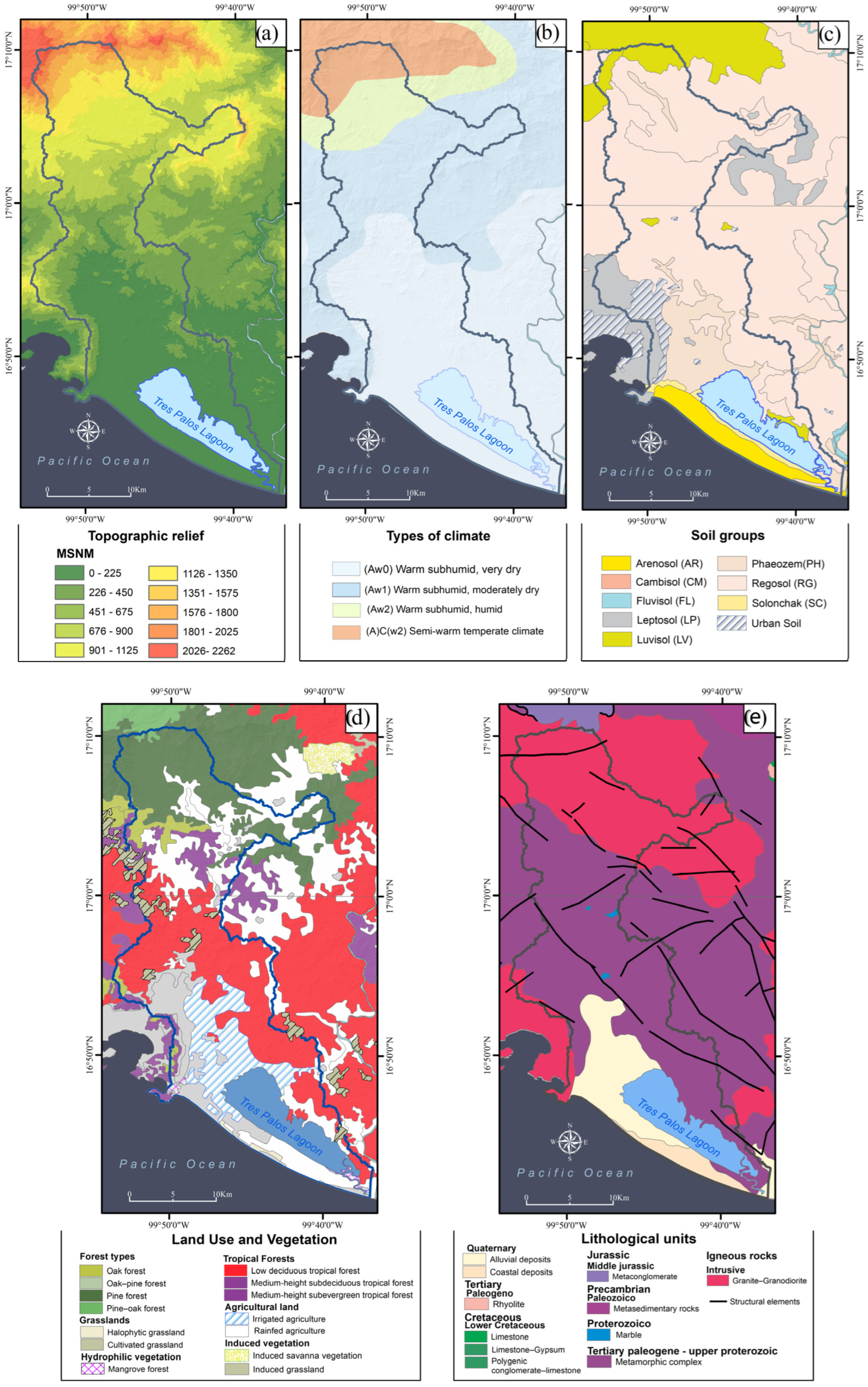
This section analyses the natural environmental components of the La Sabana River basin to understand the physical controls regulating the geomorphological and hydrological dynamics of the river system. The study integrates relief, climate, soils, vegetation, and the basin’s geological and tectonic framework, which are understood to interact in an articulated manner to generate and develop geomorphological processes. The components of the natural landscape are shown spatially in Figure 3.

3.1.1. Relief

The maximum altitude of the basin is 2262 m above sea level (masl), the lowest is 0 masl, and the average altitude is around 327 masl. The hydrographic system is located in the Southwestern Region on the Pacific coast [66]. It belongs to the Sierra Madre del Sur and, in turn, to the sub-provinces of the southern coastal mountain range and the southern coastal plain. This mountain system is characterized as a complex system composed of varied lithology, including intrusive, volcanic, sedimentary, and metamorphic rocks. The ages of the rocks range from the Precambrian to the Neogene, and their lithological units are organized by tectonic structures: folds and a system of faults and fractures [67].

In the upper reaches of the Sabana River basin, medium- and low-elevation mountains, characterized by abrupt relief due to regional tectonic activity, are the primary areas of erosion.

The basin’s territory is surrounded by the Timuchal and Veladero mountain ranges, which border the southwestern sector, adjacent to the bay of Puerto Marques. The middle and lower parts of the basin are represented by an alluvial plain formed by Quaternary deposits and delimited by mountain massifs composed of granite and granodiorite; the Tres Palos Lagoon is a prominent feature of the coastal area.

3.1.2. Climate

The climate regime of the La Sabana River basin is strongly influenced by its location on the South Pacific slope and tropical atmospheric dynamics, characterized by the marked seasonality of summer rains, the incidence of tropical waves and cyclones, and the altitudinal gradient that ranges from the coastal plain to the highest elevations, from sea level to 2200 m above sea level.

According to the Köppen climate classification [68], modified for Mexico by García [69], the basin is predominantly characterized by warm subhumid climates (Aw) with variations reflecting humidity gradients and/or orographic control dominated by the Sierra Madre del Sur mountain range. The Aw0 subtype predominates on the coastal plain, characterized by average annual temperatures above 22 °C and minimum temperatures of 18 °C, with a P/T index for summer rainfall below 43.2. The Aw1 subclimate is also present, where the P/T index ranges from 42.2 to 55.3. The Aw2 subtype is identified as the more humid areas of the basin with a P/T index greater than 55.3.

In the higher portions of the basin (>1000 m above sea level), primarily in the northwestern sector, the semi-warm subhumid climate (A)C(w2) predominates, with temperatures above 18 °C and rainfall of 40 mm in the driest month.

3.1.3. Soil

The La Sabana River basin exhibits high soil diversity, resulting from interactions among topography, fluvial dynamics, lithology, and climatic conditions across the upper reaches to the coastal zone. Soil distribution reflects a clear geomorphological gradient, with young, poorly developed soils predominating in areas of high-energy topography, and more developed soils on relatively stable or depositional surfaces.

The basin primarily contains Regosols, Leptosols, Cambisols, Phaeozems, Luvisols, Fluvisols, Arenosols, and Solonchaks, as well as localized areas of urban soils in the lower basin [70]. Regosols are the most extensive (430 km²), located on slopes and unstable surfaces within the basin, and exhibit limited horizon development with visible parent material at the surface. Leptosols (41.66 km²) are poorly developed soils in the basin, located on rocky outcrops and characterized by a rapid hydrological response. Luvisols (31.03 km²) are associated with areas of fine material accumulation and exhibit good infiltration and moisture retention. Arenosols (45.23 km²) are distributed along the coastal strip and areas near the mouth of the La Sabana River, where loose sands predominate with rapid infiltration and water retention. Solonchaks (13.09 km²) are found on the margin of the Tres Palos Lagoon and are characterized by surface salinity and poor drainage. Finally, Phaeozems (86.18 km²) are located on relatively stable surfaces and are notable for their organic matter content and good infiltration. This soil configuration has direct implications for infiltration, surface runoff, slope stability, and susceptibility to flooding, key aspects for interpreting subsequent geomorphological and hydrological analyses.

3.1.4. Vegetation

The vegetation of the La Sabana River basin exhibits a heterogeneous spatial distribution, primarily controlled by varying altitudinal gradients, the climatic regime, and the geomorphological dynamics of the river system [70]. In the higher elevation areas, characterized by mountainous terrain and moderate to steep slopes, pine, oak, and mixed forest formations predominate. These types of tree cover naturally contribute to soil conservation and protection, the regulation of surface runoff, and slope stability [71,72].

In the middle-to-upper sections of the basin, deciduous forest is dominant, with isolated areas of semi-deciduous and semi-evergreen medium-height forests. These communities reflect seasonal climatic conditions and play a moderate role in hydrological regulation, generating greater runoff during heavy rainfall events due to seasonal foliage loss [73,74].

The natural vegetation has been extensively transformed into the lower and coastal parts of the basin by agricultural uses, induced pastures, and urban areas, especially on alluvial plains and in sectors near the main channel. The presence of mangroves along the margins of the Tres Palos lagoon and at the mouth of the La Sabana River towards the Pacific is noteworthy; these ecosystems naturally act as nature-based solutions to natural hazards such as floods, tsunamis, and storm surges [75,76,77,78].

3.1.5. Regional Lithological and Tectonic Synthesis: Sierra Madre del Sur

The Sierra Madre del Sur is one of the most complex geological provinces in Mexico. It extends across the states of Colima, Jalisco, Michoacán, Guerrero, and Oaxaca, forming the watershed between the Gulf of Mexico and Pacific slopes. Its current configuration results from the interaction and accretion of various tectonostratigraphic terranes during the Mesozoic and Cenozoic eras, within the context of the subduction of the Cocos Plate beneath the North American Plate [79,80].

Among the main terranes that make up the Sierra Madre del Sur are the Mixteco, Guerrero, and Xolapa, whose lithological and structural diversity demonstrates the province’s character as a tectonostratigraphic mosaic with a highly complex paleogeographic evolution. The Mixteco terrane is also represented by the Acatlán Complex, a Paleozoic metamorphic basement composed of sequences of slates, migmatites, and ophiolites, whose deformational history records multiple phases of regional metamorphism [81]. The Guerrero terrane comprises Jurassic–Cretaceous sedimentary and volcanic sequences interpreted as fragments of an intraoceanic arc that accreted to the continental margin [82,83]. For its part, the Xolapa or Chatino terrane is defined as a high-grade plutonometamorphic belt that dominates the coastal strip of Guerrero and Oaxaca and constitutes the geological base of the Acapulco area [84,85].

3.1.6. Local Geology of the Sabana River Basin: The Xolapa Complex in Acapulco

The municipality of Acapulco sits atop the Xolapa Complex, a high-grade metamorphic core that forms the regional basement. This complex is composed primarily of granitic and granodioritic orthogneisses, psammitic-pelitic paragneisses, interbedded marbles, and migmatites, all affected by ductile deformation and amphibolite-facies metamorphism [86,87]. The most representative structures include foliations, lineations, and folds with orientations parallel to the coastline, reflecting the influence of regional tectonics on the local configuration [88].

The tectonothermal history of the Xolapa Complex in Acapulco records at least three phases of ductile deformation with associated foliations and folds, in addition to penetrative migmatization linked to the S2 foliation [89]. Chronologically, Precambrian ages are recognized, linked to the protolith of the paragneisses [90], an Early Jurassic magmatic event (~179 Ma), Early Cretaceous migmatization (~134 Ma), and thermal reactivations in the Late Cretaceous and Paleogene (~61 Ma) [85,86]. These events were followed by the intrusion of syntectonic granites (~129 Ma) and post-Laramide plutons (~55–25 Ma), which complete the magmatic evolution of the complex [90,91]. Taken together, these ages confirm that the Xolapa corresponds to a Jurassic magmatic arc accreted to the continental margin and subsequently reactivated by successive tectonic processes.

Lithologically, the Acapulco amphitheater is developed on the so-called Acapulco Trunk, a medium- to coarse-grained granitic body with porphyritic textures and phaneritic structure, whose age has been assigned from the Late Cretaceous to the Oligocene, depending on the methodology used [92].

3.2. Components of the Anthropogenic Environment

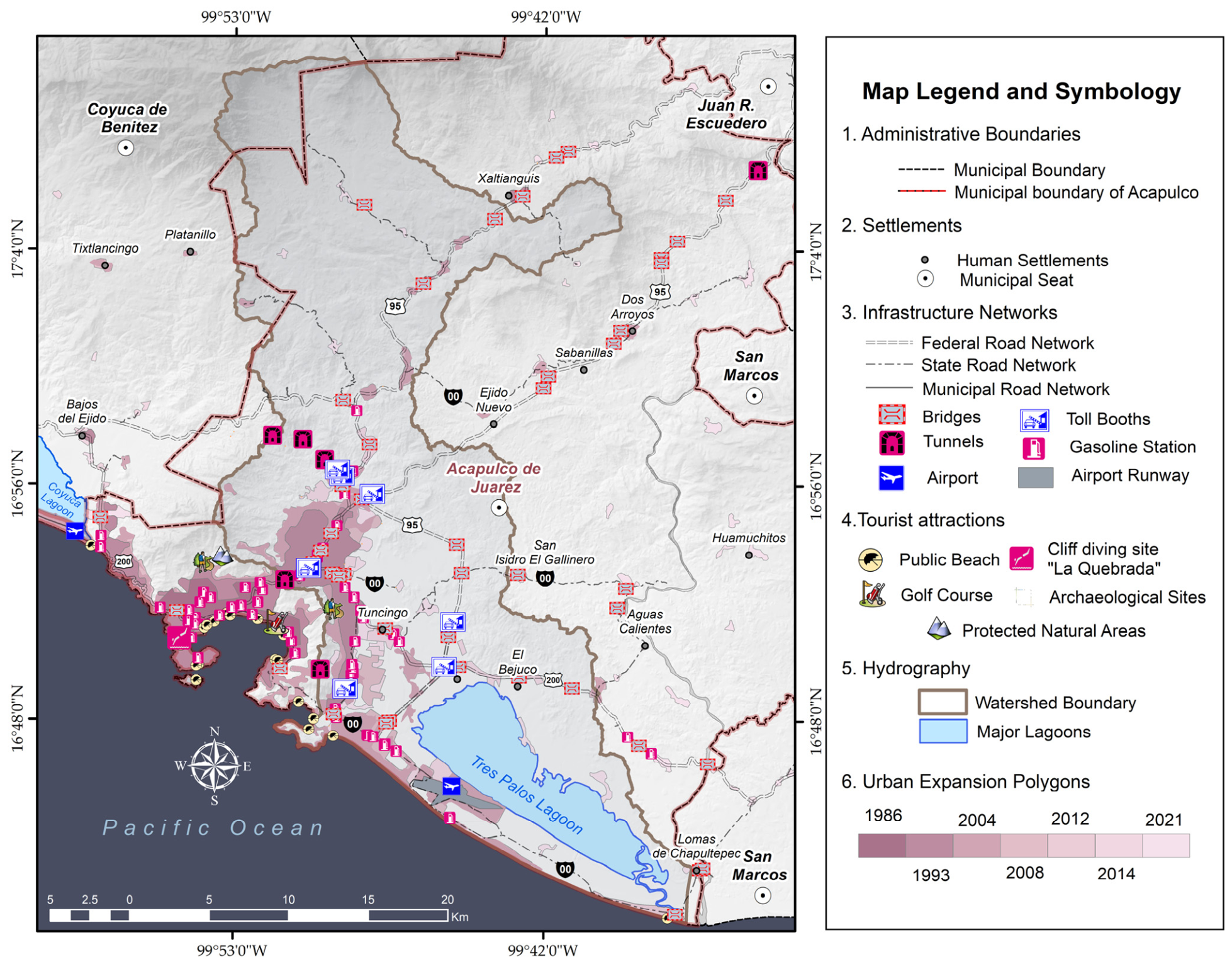
This section analyzes the main components of the anthropogenic environment of the La Sabana River basin to understand their role in transforming the basin into a territorial unit. Based on an analysis of human settlements, population, housing, and urban expansion over time, as well as road infrastructure and land use patterns, this study examines how these interventions have altered hydrological connectivity and created conditions conducive to hazardous geomorphological dynamics. The components of the natural landscape are shown spatially in Figure 4.

3.2.1. Human Settlements, Population, and Housing

Within the basin, 31 localities are identified, of which 24 are rural settlements, and 7 are urban localities [93,94]. The total number of dwellings is approximately 160,969, with an estimated population of 344,536 inhabitants. The total population represents 46.95% of the municipality of Acapulco and 9.73% of the state of Guerrero [95].

In this context, Acapulco’s urban growth shows a clear trend throughout 1984–2021, with a sustained increase in the urbanized area, which grew from 13.74 km² in 1984 to 171.63 km² in 2021. This behavior demonstrates accelerated urban expansion, particularly notable between 1984 and 2004, when the greatest increase in urbanized areas was recorded. From 2008 onward, although growth continued, a relative deceleration in the rate of expansion was observed, suggesting a gradual transition toward urban consolidation rather than strictly extensive expansion. However, the cumulative increase reflects a significant territorial transformation, with direct effects on land use, pressure on natural resources, and the geomorphological dynamics of the basin.

Human settlements tend to be located on alluvial plains, in specific areas near the main La Sabana channel, and on slopes with moderate gradients. However, there is a clear increase in housing land use on steep slopes and near ravines. This spatial configuration increases the population’s exposure to hydrometeorological events such as river flooding and flash floods caused by mudflows.

3.2.2. Road Infrastructure

Within the basin, there is an existing strategic road infrastructure with significant regional and national connectivity. Notable among these are Federal Highway 95 and its toll variant, the Autopista del Sol (95D), which connects the country’s interior to the port of Acapulco, as well as Federal Highway 200, which links the Pacific coastal corridor [96].

Among others, the development of underground road infrastructure stands out, including the Maxitúnel and the Macrotúnel (Acapulco Diamond Zone), which connect to the airport and residential areas, serving as an axis that reinforces the basin’s urban and tourist connectivity.

The internal road network comprises an estimated 1602.45 linear km of paved streets [93,94]. Despite being important for the socio-economic development of the region and bringing benefits to the population in terms of quality of life and community development, there are also environmental repercussions, including soil impermeability and altered runoff, leading to a faster hydrological response during intense precipitation events.

3.2.3. Land Use and Territorial Occupation

The land use characteristics in the basin include agricultural and urban land, with infrastructure projects intended for housing and tourism. According to the Acapulco Metropolitan Area Urban Master Plan [97] and the land use classification [70], the basin designates areas for residential, tourism, agricultural, environmental conservation, and urban infrastructure uses. In the case of Acapulco Diamante, the predominant sector with a high socioeconomic impact on the basin, technical standards stipulate that 71% of the territory is designated for environmental conservation and agricultural productivity, while the remainder should be allocated to tourism, commercial, and residential uses.

However, the presence of residential settlements in areas not designated for such use is evident, leading to the construction of homes on unstable slopes unsuitable for development [98] and in protected natural areas [99]. The Acapulco Master Plan [97] highlights cases such as irregular settlements in Valle de la Sabana, Renacimiento, or Pie de la Cuesta, where the occupation of the territory does not align with the permitted land use, thereby generating socio-environmental risks.

3.2.4. Administrative and Hydrological Framework

According to CONAGUA [100], the La Sabana River basin belongs to the Pacific South administrative region and is part of the Costa Grande de Guerrero hydrological region. This affiliation is relevant for water resource management and territorial planning of the basin, as it defines the institutional frameworks under which basin management policies, flood control, and land-use planning are implemented [101].

3.3. Hydrographic Configuration of the La Sabana River System

The La Sabana River basin is in the tropical zone of the southwestern coastal region of the Mexican Pacific. Its boundaries, defined at a scale of 1:50,000, constitute a perimeter of 210.79 km and define a surface water catchment area of 740.11 km². Internal differentiation of the hydrographic system allowed the identification of 24 sub-basins, 10 of which drain directly into the Tres Palos Lagoon, while the remaining 14 have internal drainage.

The basin’s morphology, viewed from a two-dimensional plane, is asymmetrical, as the watershed follows an irregular pattern with sinuous, uneven contours. This condition is also reflected in the drainage organization, resulting in differential development of the network, with a higher density of tributaries on the western slope than on the eastern slope, suggesting the influence of a well-defined tectonic structure. The hydrological network of the basin developed on basements composed of granite-granodiorite and metamorphic units formed during the Paleozoic, Tertiary, Paleogene, and Upper Proterozoic. It is characterized by main rivers averaging 9.5 km in length and an average drainage density of 4.7 km/km². These characteristics have favored the development of predominantly detrital patterns; however, the presence of faults and regional lineaments conditions the orientation of the channels, giving rise to sectors with subdentric and subparallel patterns.

The fluvial system reaches order 7, with the La Sabana River as the highest-order river. Drainage systems of orders 5, 6, and 7 are influenced by tectonic processes, while those of orders lower than 4 tend to be associated with erosional processes and are in the headwaters of the sub-basins, where steep slopes are prominent. The La Sabana River is the main channel of the basin and has a total length of 66.75 km, extending from the basin’s headwaters at Cerro de San Nicolás, at approximately 2262 m above sea level, to its mouth at the Tres Palos Lagoon. Along this stretch, the channel reaches drainage order 7, which is recognized from the town of km 48 and is maintained until its mouth.

In the upper part of the basin, the main channel is consolidated by the confluence of two important streams: firstly, the Potrerillos River, which flows near the town of km 48, and secondly, the Moyoapa River, which flows near the town of km 39. These confluences define the La Sabana River as the main collector, concentrating the runoff and conveying water flows from the mountains to the coastal plain. According to the National Water Commission in Mexico (2024), the water resources of the La Sabana aquifer have an average annual availability of 35,220,061 m³. The average annual recharge received by the aquifer amounts to 92,000,000 m³, comprising approximately 72,900,000 m³/year of vertical recharge from rainfall and infiltration, as well as 19,100,000 m³/year of horizontal groundwater inflow.

Regarding surface water, the aquifer is estimated to contribute approximately 11,000,000 m³/year of base flow to the La Sabana River basin. However, it is important to note that the water supply of the urban and tourist area of the basin does not depend entirely on this aquifer, as it also uses external sources such as the Papagayo River, where the current registered exploitation reaches an extraction volume of 35,579,939 m³ per year, according to the Public Registry of Water Rights 2022 [102].

3.4. Indicators of the Sub-Basins of the La Sabana River

The morphometric indicators of the La Sabana River sub-basins (

Table 4. Morphometric index values of the 24 sub-basins of the Rio la Sabana basin.

Index	S1	S2	S3	S4	S5	S6	S7	S8	S9	S10	S11	S12	S13	S14	S15	S16	S17	S18	S19	S20	S21	S22	S23	S24
A	24.2	22.7	28.4	72.7	30	47.5	61.1	25.7	13.6	14.2	22.4	20.4	15.5	12.6	21.7	16.1	21.9	8	5.5	13.3	12.1	3.04	5.3	9.4
P	33.7	31.8	47.5	67.3	55.5	49.4	66.2	36.4	24.6	26.7	37.1	35.2	29.7	35	29.3	21.6	43.5	14.8	12.4	27.3	27.1	8.3	12.4	25.3
Lb	8.1	6.7	10.3	16.7	15.7	9.1	13.5	6.9	5.3	7.8	8.2	7.5	6.1	8.2	8.1	2.1	8.3	4.1	4.1	5.5	5.3	1.9	3.2	1.9
Wb	3.2	6.3	3.3	5.7	2.9	8.6	4.9	6.1	3.5	2.5	3.6	3.6	4.1	0.9	3	8.3	3.3	2.8	1.6	3.5	4.1	2.1	3.1	10.2
Re	0.7	0.8	0.6	0.6	0.4	0.85	0.65	0.8	0.8	0.55	0.65	0.6	0.7	0.5	0.65	0.9	0.6	0.8	0.65	0.75	0.7	1	0.8	0.4
Ff	0.4	0.5	0.3	0.3	0.1	0.6	0.3	0.5	0.5	0.2	0.3	0.4	0.4	0.2	0.3	0.7	0.3	0.5	0.3	0.4	0.4	0.8	0.5	0.1
U	6	5	5	6	5	6	6	5	5	5	5	5	5	4	5	4	5	4	3	5	4	3	4	4
Nu	809	714	917	2439	892	1465	1923	730	387	374	632	646	509	346	593	413	634	192	102	337	361	67	131	244
Tls	125.9	116.2	136.8	391.4	149.7	233.9	316.6	128.6	62.2	70.1	108.6	109.9	78	61.3	116.7	81.7	110.1	37.6	21.8	59.6	55.1	11.8	21.3	39.2
Lu	2.9	7.4	15.4	22.7	18.8	17.2	23.8	7.8	6.4	8.7	12.3	11.4	9.1	9.8	9.4	2.3	13.3	4.3	1.6	8.2	8.6	2.1	1.8	2.3
Rb	1.9	2.1	1.8	1.9	1.6	1.7	1.7	2	1.9	2.8	1.7	2.1	1.9	1.7	2.7	2	1.8	1.8	1.5	2.2	1.8	2.1	1.7	1.6
Fs	33.3	31.5	32.2	33.5	29.7	30.8	31.4	28.3	28.3	26.2	28.1	31.6	32.7	27.4	27.2	25.5	28.8	23.9	18.4	25.2	29.9	22.1	24.5	25.9
Dt	23.9	22.4	19.3	36.2	16	29.6	29	20	15.7	14	17	18.3	17	9.8	20.1	19.7	14.5	12.9	8.1	12.3	13.3	8.1	10.5	9.6
Dd	5.2	5.1	4.8	5.3	4.9	4.9	5.1	4.9	4.5	4.9	4.8	5.4	5	4.8	5.3	5	5	4.7	3.9	4.4	4.5	3.8	3.9	4.1
Hmax	1142	383	1468	2262	1987	743	1122	465	607	663	480	430	239	940	860	445	310	320	224	288	164	124	106	103
Hmin	474	941	474	384	376	93	96	33	33	31	23	23	19	19	15	0	0	0	0	1	0	13	18	6
Er	668	558	994	1878	1611	650	1026	432	574	632	385	407	220	921	845	445	310	320	224	287	164	111	88	97
Sm	13.3	13.21	8.9	12.5	13.6	11.9	10.9	13.4	15.5	12.9	8.1	9.3	9.1	10.8	13.3	13.9	6.2	12.8	12.1	9.2	5.4	3.1	5.9	4.3
Rr	82.4	83.2	96.5	112.5	102.6	71.43	76	62.6	108.3	81.03	46.95	54.2	36	112.3	104.3	211.9	37.3	78	54.6	52.1	30.9	58.4	27.5	51

Note: A, área de la subcuenca (km²); P, perímetro (km); Lb, longitud máxima de la cuenca (km); Wb, ancho medio de la cuenca (km); Re, relación de elongación (adimensional); Ff, factor de forma (adimensional); U, orden máximo de drenaje (n); Nu, número total de cauces (n); Tls, longitud total de la red de drenaje (km); Lu, longitud total del cauce (km); Rb, relación de bifurcación (adimensional); Fs, frecuencia de corrientes (n/km²); Dt, textura de drenaje (n); Dd, densidad de drenaje (km/km²); Hmax, elevación máxima (m); Hmin, elevación mínima (m); Er, energía del relieve (m); Sm, pendiente media (°); Rr, relación de relieve (m/km).

) show a marked spatial variability in size, drainage organization, and topographic relief conditions. The basin areas range from 3.04 km², reflecting a heterogeneous hydrographic structure composed of small coastal units and larger basins in the upper part of the watershed. The indicators associated with the drainage network indicate a well-developed hydrological system, with high stream frequency (18.4–33.5 n/km²) and drainage density (3.8–5.4 km/km²), revealing efficient runoff concentration in most sub-basins.

Regarding topographic relief, very pronounced altitudinal contrasts are observed, with differences ranging from 120 m in the lowlands to 1800 m in the mountainous sectors, indicating high variability in relief energy. Consistently, this relationship is evident in the mean slope values (3.1–15.5°), which reflect a transition from relatively stable terrain sectors to areas with steeper slopes, indicating greater erosive activity. These variations highlight the existence of differentiated hydrogeomorphological conditions within the basin, which are analyzed in greater detail in the following sections.

3.4.1. Basin Geometry

The geometry of the sub-basins in the La Sabana River basin was evaluated using the complementary set of shape factor (Ff) and elongation ratio (Re) indicators to recognize the hydrological response potential [103]. These indices were calculated from the attributes of each sub-basin (A, P, and Lb).

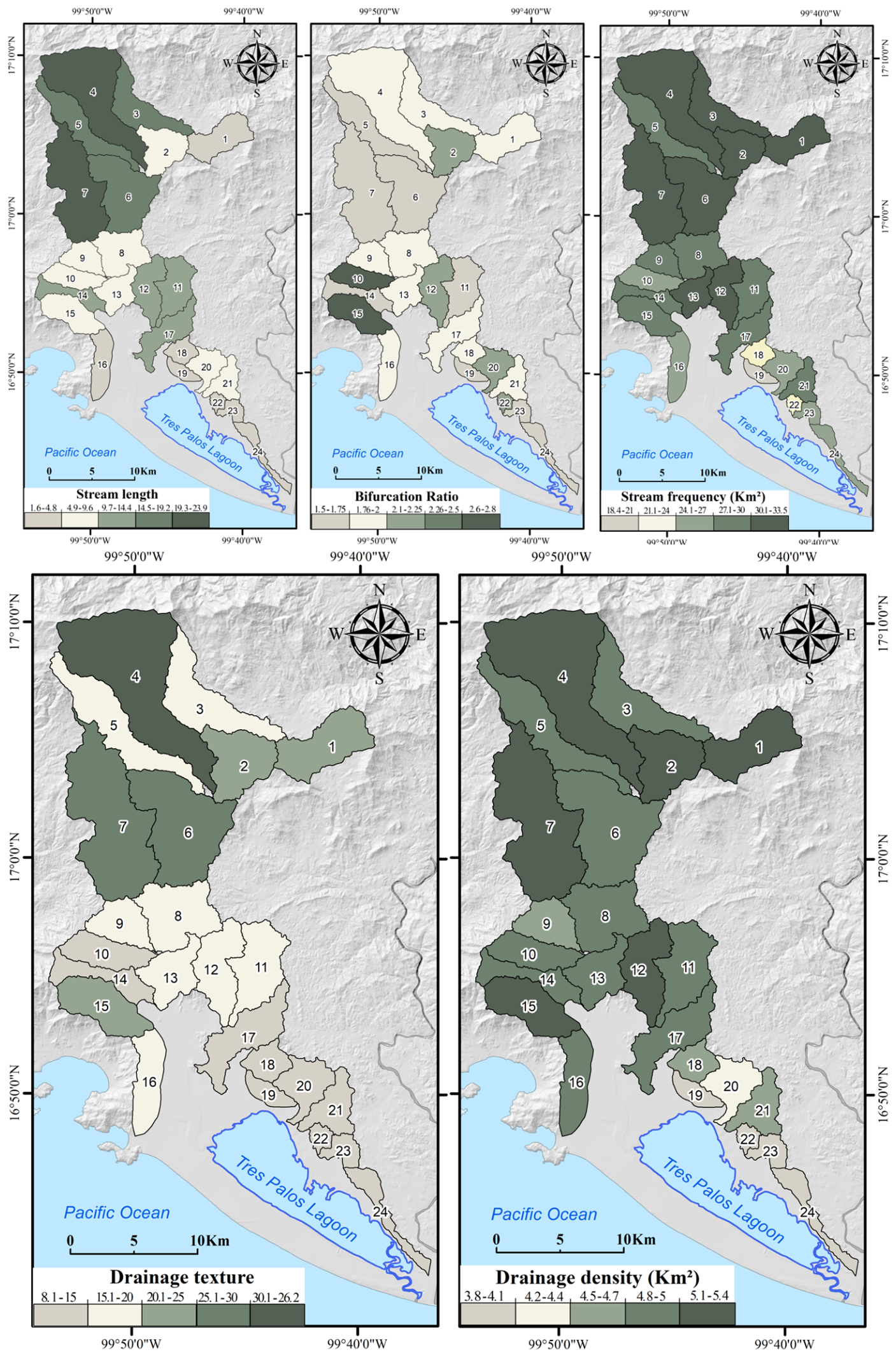
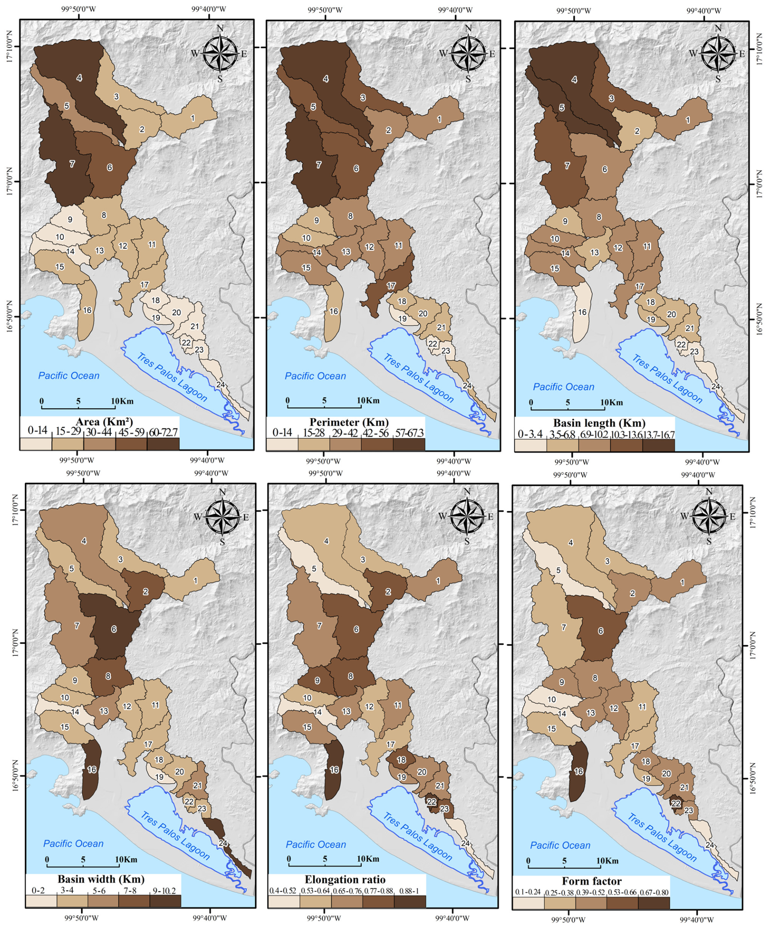
On the one hand, the elongation ratio characterizes the basin’s geometry, defined as the ratio of the basin area to the square of its maximum length [104]. The range of values for the elongation ratio is between 0 and 1; the closer to 1, the more circular the basin geometry. Basins can be classified into four groups: elongated (<0.5), slightly elongated (0.5–0.7), oval (0.7–0.8), and circular (≤0.8) [105]. The Re values for the sub-basins range from 0.4 to 1, with a higher concentration between 0.6 and 0.8; these values indicate moderate elongation for most sub-basins. The lowest values are recorded for sub-basins S5 (0.4) and S24 (0.5), while the highest are for sub-basins S6 and S22 (0.85). Specifically, sub-basin S22 is at the extreme threshold of the analyzed set with a value of 1.

On the other hand, the shape factor (Ff) refers to the consistency of the basin’s watershed and is the result of the relative relationship between the total basin area and the square of its length [56]. Sub-basins with high values are characterized by a flow that concentrates water more quickly, while those with low values distribute the flow more slowly and steadily.

The results for this indicator range from 0.1 to 0.8; values between 0.1 and 0.4 are the lowest and correspond to elongated geometric configurations, as seen in sub-basins 5, 10, 14, 15, and 24, indicating higher flow intensity over short periods. The highest values (Ff ≥ 0.6) are recorded in sub-basins S6, S16, and S18 and are associated with more compact geometries (Figure 5).

3.4.2. Drainage Network

Drainage network analysis is fundamental to the study of watersheds, as it enables understanding of the organization and functioning of the river system [104]. The results of the drainage network morphometric indices are organized into three thematic blocks: network hierarchy and organization (U, Un, and Rb), drainage pattern development (Tls and Lu), and drainage density and texture (Fs, Dt, and Dd). The values obtained for the La Sabana River sub-basins show significant variations in the organization and hierarchy of the river system. These variations indicate areas with a greater capacity to concentrate surface runoff within the study area.

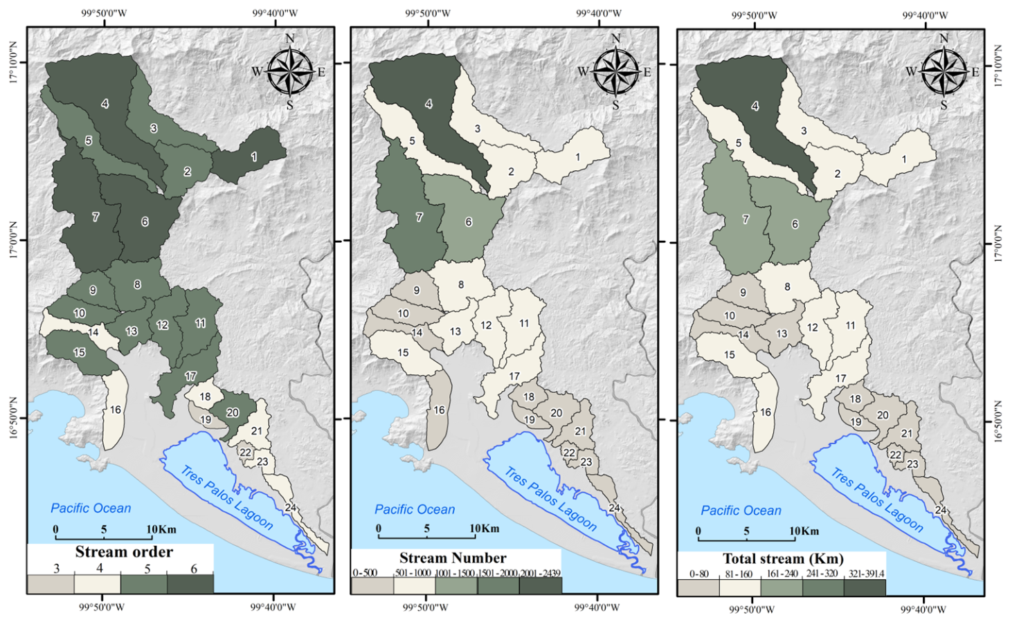
The classification of drainage order (U), based on the criteria established by Strahler [30], ranges from third to sixth order at the sub-basin level. Based on drainage development, this result indicates structural contrasts [57]. The sub-basins that reach order six are S1, S4, S6, and S7, reflecting the development of a more integrated drainage system under tectonic control. Sub-basins S19 and S22, on the other hand, exhibit order three, the lowest hierarchy, and are associated with hydrological development driven by erosional processes.

The bifurcation ratio (Rb) ranges from 1.5 to 2.7, initially suggesting moderate branching in surface hydrological development. However, sub-basins S10 and S15, which show the highest values (2.8 and 2.7), indicate the development of their drainage networks over mountainous terrain with moderate to steep slopes and rapid flood response in flow rates.

The total channel length (Tls) expresses the total length of the drainage system, and the values in the sub-basins of this study range from 11.8 km to 394.4 km. Sub-basins S4, S6, and S7 stand out for having the greatest lengths, which likely correspond to larger areas of development and more integrated networks, in contrast to the smaller sub-basins with the shortest lengths. Regarding the length of the main channel (Lu), sub-basin S16 revealed a length of 1.6 km, and sub-basin S7 a length of 23.8 km.

The drainage density and texture indicators have revealed a high degree of surface dissection for most sub-basins. On the one hand, the stream frequency index (Fs) ranges from 22 to 33 km/km², while the density (Dd) ranges from 3.8 to 5.4 km/km². These results demonstrate relatively dense and well-integrated drainage patterns that efficiently convey surface runoff (Figure 6).

3.4.3. Topographic Relief

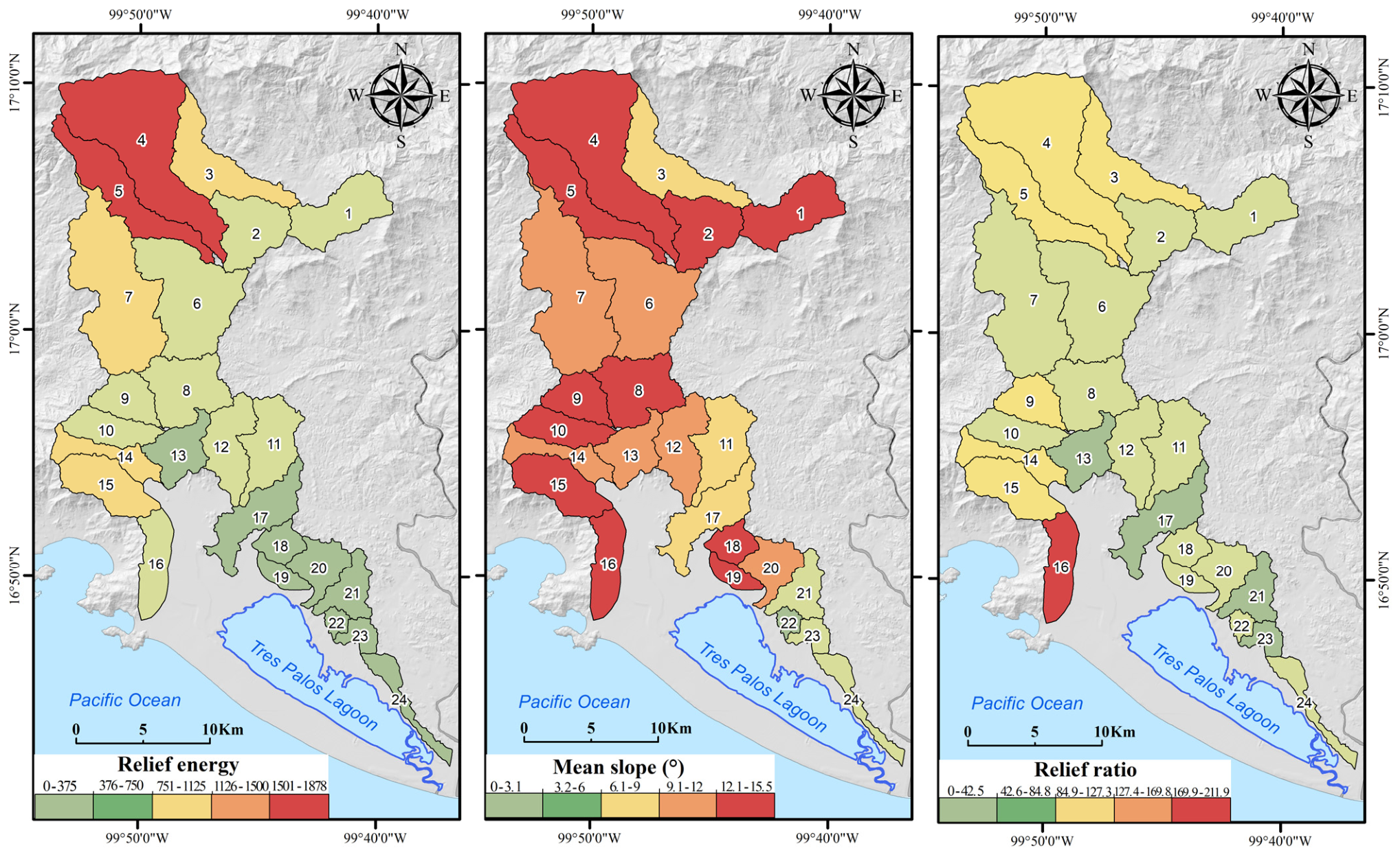
The spatial distribution of basin morphometric indices associated with topographic relief (Figure 7) has allowed for the identification of distinct stages in the morphodynamic development of the sub-basins, based on relief energy (Er), average slope (Sm), and relief ratio (Rr).

The findings reveal marked contrasts in the relief of the sub-basins. Maximum altitudes (Hmax) range from 103 to 2262 m, while minimum altitudes range from 0 to 474 m. The spatial distribution of these values validated the proposed geomorphological regionalization for the basin, differentiating the upper, middle, and lower sectors.

Relief energy (R) was calculated as the maximum altitude difference within each drainage unit [47]. Values range from 88 to 1878 m in the study area, with intensities exceeding 1000 m concentrated in the upper basin region, particularly in S4, S3, S5, and S7. These units are characterized by the most active erosion processes, due to deeply dissected valleys with slopes greater than 60°.

In contrast, S22, S23, and S24 exhibit values below 120 m, indicating apparent stability, gentle slopes, and a predominance of accumulation and sedimentation processes. Average slope values (Sm) range from 3.1° to 15.5°, with the highest values recorded in S9, S16, and S18, and the lowest in S22, S21, and S24.

Finally, the calculation of the relief relationship (Rr) links relief energy (Er) with the maximum length of the basin (Lb). The results cover the range from 27.5 m/km to 211.9 m/km. Sub-basins S4, S14, and S16 exhibit the highest values and give rise to areas with high mountains and short lengths; this means that runoff from the main channel descends too quickly before precipitation occurs.

3.4.4. Time of Concentration

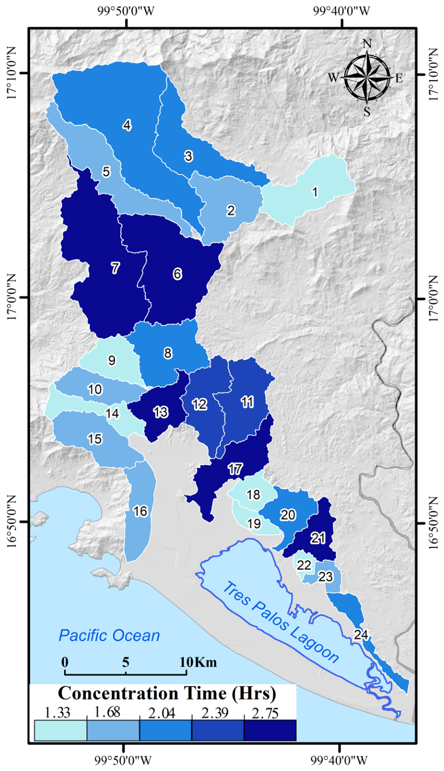
The time of concentration (Tc) estimated using Giandotti’s formula [64], ranged from 0.98 to 2.75 h, indicating a predominantly rapid hydrological response in the sub-basins that make up the La Sabana River basin.

The sub-basins with the shortest concentration are S19 (0.98 h), S14 (1.19 h), S22 (1.20 h), S1 (1.16 h), S16 (1.16 h), and S18 (1.24 h). These units are characterized by small spatial dimensions and shorter main channel lengths, which favour an accelerated concentration of surface runoff. In contrast, the sub-basins with the longest concentration times include S17 (2.75 h), S6 (2.62 h), S7 (2.61 h), S13 (2.48 h), and S11 (2.39 h), which exhibit greater structural development of the drainage system and longer flow lengths in the main channel, increasing the time required for water to reach the outlet.

The spatial distribution of Tc reveals that the river system comprises sub-basins with varying levels of flow concentration efficiency, with higher values in the middle part of the basin and lower values dominating smaller coastal sub-basins. This results in contrasts in the rate at which each contributes to the main channel flow during rainfall (Figure 8).

3.4.5. Hypsometric Index Estimation and Hypsometric Curve Analysis

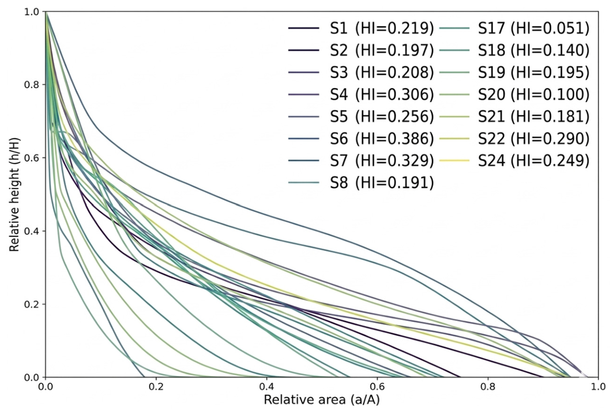
The hypsometric index values for the basin range from 0.040 (S13) to 0.386 (S6). These results reflect advanced geomorphological evolution in the analyzed units (Figure 9). In morphodynamic terms, these values indicate that most sub-basins have undergone progressive, continuous denudation. Although the basin’s relief energy is 2262 m, the average value across the basin is 496 m, reinforcing the idea of a geomorphologically evolved landscape. In contrast, sub-basins S6 (0.386), S7 (0.329), and S4 (0.306) exhibit relatively higher values for the hypsometric integral index, indicating the presence of morphological features that are likely preserved compared to the other sub-basins.

3.5. Correlation Matrix Between Morphometric Indicators

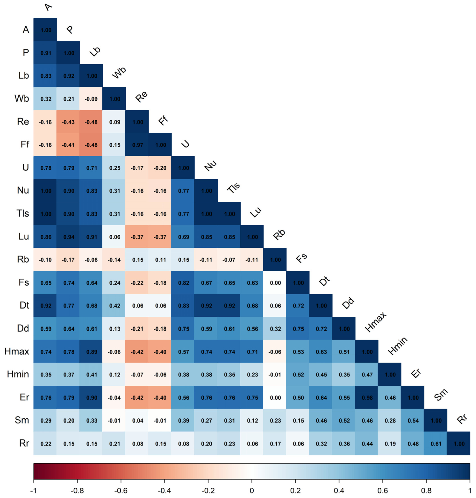
The evaluation of interdependence among the morphometric indices calculated for the La Sabana River sub-basins was conducted using a Pearson correlation matrix, with a threshold of r ≥ 0.7 for the analyzed variables. The matrix reveals a pattern of high collinearity between the indicators associated with basin geometry and the drainage network, as shown in Figure 10.

In particular, the basin area (A) shows perfect correlations (r ≈ 0.99) with the total channel length (Tls) and the number of streams (Nu), indicating that the drainage system tends to develop more fully in larger sub-basins. Furthermore, the perimeter (P), basin length (Lb), and main channel length (Lu) are strongly associated (r > 0.90), forming a group of variables that represent the spatial dimensions of the sub-basins. The shape parameters, specifically the elongation ratio (Re) and shape factor (Ff), have been confirmed in their results to describe the consistency of sub-basins’ geometric characteristics, with correlation coefficients r > 0.97.

The index that showed low values was the bifurcation ratio (Rb), in contrast to most other variables. This occurs because drainage develops in a resistant lithological context, dominated by granitic rocks and metamorphic complexes, and is controlled by fractures that govern the organization and development of the fluvial system.

Morphodynamic processes are reflected in the relationship between the maximum elevation (Hmax) of the sub-basins and the relief energy (Er), yielding r values > 0.98. Furthermore, moderate-to-strong associations are maintained with drainage density (Dd) and drainage texture (Dt), indicating that relief characteristics determine the structure and degree of drainage development.

The strong collinearity among the variables analyzed, as shown in the correlation matrix, suggests implementing principal component analysis as a statistical technique. This allows for dimensionality reduction in the morphometric indicators and helps understand the dominant patterns in the sub-basins comprising the La Sabana River basin.

The strong collinearity among the variables, as indicated by the correlation matrix, suggests using principal component analysis to reduce the dimensionality of the morphometric indicators and to identify dominant patterns across the sub-basins that make up the La Sabana River basin.

3.6. Analysis and Interpretation of Principal Components

The high degree of correlation among the morphometric indicators prompted the use of Principal Component Analysis (PCA) to identify the variables influencing the hydrological functioning and morphological development of the La Sabana River sub-basins.

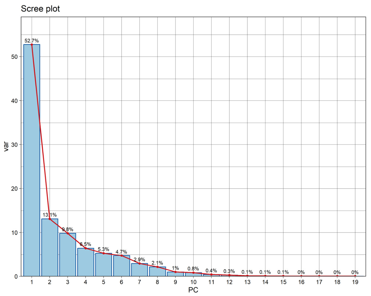
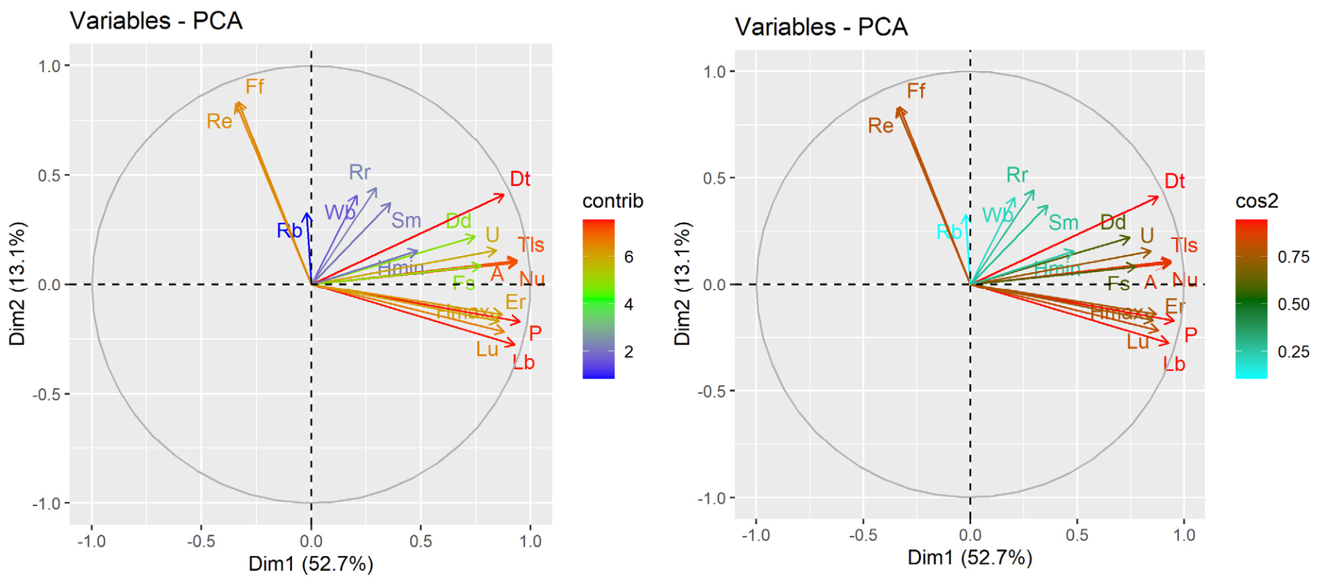
Principal component analysis synthesized the results of the 19 indicators examined in this study into two factorial dimensions (principal components) that represent the dominant structure of the fluvial system associated with the basin’s geometry, hydrological network, and relief. The scree plot shows an abrupt inflection point between dimensions 1 and 2, which represent the components capturing the largest proportion of variance in the evaluated indicators, as shown in Figure 11. Subsequent components, on the other hand, have individual contributions of less than 10% and provide residual information.

The first principal component explains 52.7% of the total variance (eigenvalue = 10.02), while the second explains 13.1% (eigenvalue = 2.49), together accounting for 65.8% of the variability in the indices. Applying the Kaiser criterion (eigenvalue > 1) [106], five components meet this threshold (PC1–PC5, with eigenvalues of 10.02, 2.49, 1.87, 1.23, and 1.01, respectively), collectively explaining 87.5% of the total variance. Nevertheless, the pronounced inflection in the scree plot between PC1 and PC2, combined with the interpretive clarity of these two dimensions, supports retaining only PC1 and PC2 to evaluate the dominant hydrogeomorphological controls. The complete eigenvalue structure of all 19 components is presented in

Table 5. Eigenvalues and explained variance of the principal components obtained from PCA of morphometric indicators of the La Sabana River sub-basins.

Component	Eigenvalue	% Variance	Cumulative %
PC1	10.022	52.747	52.747
PC2	2.492	13.114	65.86
PC3	1.865	9.818	75.679
PC4	1.23	6.472	82.151
PC5	1.009	5.312	87.463
PC6	0.902	4.748	92.211
PC7	0.555	2.919	95.13
PC8	0.408	2.147	97.276
PC9	0.187	0.986	98.262
PC10–PC19	<0.158	<0.832	100

.

Principal component analysis shows that PC1 (Dim1) is dominated by indicators associated with the size and drainage network of the basin, particularly the area (A), total channel length (Tls), number of streams (Nu), perimeter (P), main channel length (Lu), and maximum basin length (Lb), which represent high values in the contribution and cos² graphs, as shown in Figure 12. On the other hand, PC2 (Dim2) is primarily influenced by basin-shape indicators, particularly the elongation ratio (Re) and the factor (Ff). These variables contribute significantly to the vertical axis and have orientations opposite to those of PCA1, indicating that PC2 captures independent variation in sub-basin size. Variables such as Rr, Sm, and Wb contribute partially to this component, suggesting a dimension related to geometric configuration and relative dissection.

4. Discussion

The results reveal a hydrogeomorphological structure highly susceptible to hazardous geomorphological processes during extreme hydrometeorological events. The drainage density values (3.8–5.4 km/km²) are consistent with those reported in tropical coastal basins prone to flash floods [15,16,17], and contrast sharply with values reported in basins where permeable substrate and moderate relief produce slower hydrological responses, such as the Son Basin in India (0.26 km/km²) [19].

Studies conducted in Nepal [23] and Thailand [24] similarly identified drainage density and relief ratio as primary controls on flash-flood potential, thereby confirming the dominant control of CP1 in this research. The concentration times obtained (0.98–2.75 h) place the basin within a range of rapid hydrological response, consistent with previous studies documenting that basins with Tc below 1.5 h generate high, short-duration flow peaks, substantially reducing the available warning windows [14,21].

The hypsometric index values (0.04–0.388) indicate an advanced geomorphological evolution in most of the sub-basins, while the upper basin units S4, S6, and S7 retain active morphodynamic characteristics associated with the generation of sediments during extreme rainfall [32].

This research has reported patterns comparable to those found in mountainous sub-basins of southern Italy, where morphometric parameters allowed for the differentiation of multi-hazard dynamics [27]. Similarly, in the Western Ghats of India, it was documented that the basement’s geological structure controls the organization and pattern of the drainage network [20], consistent with the structural influence of the Xolapa Complex on the La Sabana River drainage network.

The PCA structure, with PC1 (52.7%) associated with basin size and drainage network and PC2 (13.1%) with basin shape, is consistent with previous studies that identified drainage density, slope, and basin topography as dominant morphometric controls on flood susceptibility [28,29,107].

From a methodological perspective, several limitations must be acknowledged. The static 15 m digital elevation model (DEM) does not capture topographic changes following recent cyclone-induced events, a limitation recognized as critical in morphometric flood studies [26]. The absence of rainfall frequency analysis and hydrodynamic modeling limits the transition from susceptibility-based interpretations to quantitative hazard assessments; previous research has shown that integrating the SCS-CN model (Soil Conservation Service curve) with synthetic unit hydrographs substantially improves predictive capacity in basins without gauging stations [24], an approach that future research in La Sabana should incorporate.

Regarding the hypsometric integral, its use in this study was strictly limited to characterizing the relative geomorphological evolutionary stage of each sub-basin [60,61], without attempting to discriminate between tectonic, climatic, or lithological controls on fluvial relief.

It is important to note that the small size of the sub-basins limits the accuracy of automated drainage extraction at 15 m resolution; therefore, morphometric results in small sub-basins should be interpreted with caution.

Identifying sub-basins with Tc ≤ 1.5 h provides a spatially explicit basis for prioritizing early warning systems and land-use regulation [11,12]. The overlap between high morphometric susceptibility and existing settlements on floodplains and unstable slopes [98,99] reveals a persistent gap between scientific knowledge and its incorporation into planning instruments, a recognized challenge in tropical coastal governance [9,10]. Similar conclusions have been reached in comparable contexts, recommending morphometric analysis as a practical tool for sub-basin-level flood mitigation in the absence of historical records [107]. The replicability of the proposed framework, using open data and freely available tools, increases its potential for institutional adoption, and its application could be extended to other coastal basins exposed to cyclones, thereby providing a scientific basis for sustainable land-use planning and disaster risk reduction [36].

5. Conclusions

This study developed an integrated physical–geographic and multivariate framework to analyze the geomorphological and multi-hazard dynamics associated with tropical storms in the coastal La Sabana River basin in southern Mexico. The combined assessment of morphometric parameters, physical–environmental conditions, and their synthesis through principal component analysis (PCA) demonstrated that susceptibility to coupled hazards—particularly floods and landslides—is not controlled by isolated factors, but by the interaction between basin geometry, drainage network hierarchy, relief configuration, and patterns of urban expansion in vulnerable zones such as alluvial plains and unstable slopes.

In morphometric terms, the high drainage density (average 4.7 km/km²), the predominance of short concentration times (0.98–2.75 h), and the PCA structure—explaining 65.8% of the variance in two components associated with basin size and drainage organization—indicate that the system has a high capacity for rapid runoff concentration and efficient flow propagation. Sub-basins with Tc ≤ 1.5 h emerge as priority units due to their greater predisposition to rapid hydrological response under extreme rainfall conditions.

From a multi-hazard perspective, the results highlight that coastal location and basin compactness can enhance hydrological responsiveness even in areas with lower relative relief, emphasizing that hazard potential results from interacting geomorphological controls rather than from single morphometric indicators. This confirms that morphometric and multivariate analyses provide a robust basis for identifying spatial patterns of susceptibility in complex environments where hydrological and slope processes converge.

From a coastal risk governance perspective, the study provides a spatially explicit and methodologically reproducible framework to support land-use planning, risk-informed zoning, and the design of early warning systems at the sub-basin scale. The use of open-access geospatial data and reproducible analytical procedures enhances the applicability of the approach in tropical coastal regions with limited technical and institutional capacities.

Finally, future research should incorporate hydrometric observations and extreme precipitation frequency analyses to validate and extend the proposed framework toward quantitative assessments of multi-hazard risk. Integrating morphometric analysis with hydroclimatic and geotechnical variables will be essential to advance from susceptibility-based interpretations toward predictive models of geomorphological response under changing environmental.

References

1. Laignel, B.; Vignudelli, S.; Almar, R.; Becker, M.; Bentamy, A.; Benveniste, J.; Birol, F.; Frappart, F.; Idier, D.; Salameh, E.; et al. Observation of the coastal areas, estuaries and deltas from space. Surv. Geophys. 2023, 44, 1309–1356. [Google Scholar] [CrossRef]
2. Ward, N.D.; Megonigal, J.P.; Bond-Lamberty, B.; Bailey, V.L.; Butman, D.; Canuel, E.A.; Diefenderfer, H.; Ganju, N.K.; Goñi, M.A.; Graham, E.B.; et al. Representing the function and sensitivity of coastal interfaces in Earth system models. Nat. Commun. 2020, 11, 2458. [Google Scholar] [CrossRef]
3. Kron, W. Coasts: The high-risk areas of the world. Nat. Hazards 2013, 66, 1363–1382. [Google Scholar] [CrossRef]
4. Melet, A.; Teatini, P.; Le Cozannet, G.; Jamet, C.; Conversi, A.; Benveniste, J.; Almar, R. Earth observations for monitoring marine coastal hazards and their drivers. Surv. Geophys. 2020, 41, 1489–1534. [Google Scholar] [CrossRef]
5. Lai, Y.; Li, J.; Gu, X.; Liu, C.; Chen, Y.D. Global compound floods from precipitation and storm surge: Hazards and the roles of cyclones. J. Clim. 2021, 34, 8319–8339. [Google Scholar] [CrossRef]
6. Lazarus, E.D.; Ellis, M.A.; Murray, A.B.; Hall, D.M. An evolving research agenda for human–coastal systems. Geomorphology 2016, 256, 81–90. [Google Scholar] [CrossRef]
7. Zúñiga, E.; Magaña, V. Vulnerability and risk to intense rainfall in Mexico: The effect of land use cover change. Investig. Geográficas 2018, 95, 1–18. [Google Scholar] [CrossRef]
8. Rentschler, J.; Avner, P.; Marconcini, M.; Su, R.; Strano, E.; Vousdoukas, M.; Hallegatte, S. Global evidence of rapid urban growth in flood zones since 1985. Nature 2023, 622, 87–92. [Google Scholar] [CrossRef]
9. Zanin, G.M.; Barbanente, A.; Romagnoli, C.; Parisi, A.; Archetti, R. Traditional vs. novel approaches to coastal risk management: A review and insights from Italy. J. Environ. Manag. 2023, 346, 119003. [Google Scholar] [CrossRef] [PubMed]
10. Cienfuegos, R. Flood risk from geophysical and hydroclimatic hazards: An essential integration for disaster risk management and climate change adaptation in the coastal zone. Nat. Hazards 2023, 119, 1113–1115. [Google Scholar] [CrossRef]
11. Carapuço, M.M.; Taborda, R.; Andrade, C.; de Jonge, V.N. How to foster scientific knowledge integration in coastal management. Ocean. Coast. Manag. 2021, 209, 105661. [Google Scholar] [CrossRef]
12. Pasquier, U.; Few, R.; Goulden, M.C.; Hooton, S.; He, Y.; Hiscock, K.M. “We can’t do it on our own!”—Integrating stakeholder and scientific knowledge of future flood risk to inform climate change adaptation planning in a coastal region. Environ. Sci. Policy 2020, 103, 50–57. [Google Scholar] [CrossRef]
13. Obeidat, M.; Awawdeh, M.; Al-Hantouli, F. Morphometric analysis and prioritisation of watersheds for flood risk management in Wadi Easal Basin (WEB), Jordan, using geospatial technologies. J. Flood Risk Manag. 2021, 14, e12711. [Google Scholar] [CrossRef]
14. Garzon, L.F.L.; Johnson, M.F.; Mount, N.; Gomez, H. Exploring the effects of catchment morphometry on overland flow response to extreme rainfall using a 2D hydraulic-hydrological model (IBER). J. Hydrol. 2023, 627, 130405. [Google Scholar] [CrossRef]
15. Alam, A.; Ahmed, B.; Sammonds, P. Flash flood susceptibility assessment using the parameters of drainage basin morphometry in SE Bangladesh. Quat. Int. 2021, 575, 295–307. [Google Scholar] [CrossRef]
16. Chissende, A.; Mehmood, M.S.; Huo, A.; Lou, P.; Wang, Z. Riverine flood susceptibility assessment using drainage basin morphometry in the Bahe River. Int. J. Disaster Risk Reduct. 2025, 117, 105181. [Google Scholar] [CrossRef]
17. Melsse, D.W.; Tegegne, M.A.; Mekonnen, Y.A.; Bihon, Y.T. Morphometric analysis for understanding river basin hydrology: A case of gelda watershed, Tana Sub-Basin, Ethiopia. Appl. Water Sci. 2025, 15, 171. [Google Scholar] [CrossRef]
18. Salhi, A.; El Hasnaoui, Y.; Cutillas, P.P.; Heggy, E. Soil erosion and hydroclimatic hazards in major African port cities: The case study of Tangier. Sci. Rep. 2023, 13, 13158. [Google Scholar] [CrossRef]
19. Rai, P.K.; Mishra, V.N.; Mohan, K. A study of morphometric evaluation of the Son basin, India using geospatial approach. Remote Sens. Appl. Soc. Environ. 2017, 7, 9–20. [Google Scholar]
20. Thomas, J.; Joseph, S.; Thrivikramaji, K. Morphometric aspects of a small tropical mountain river system, the southern Western Ghats, India. Int. J. Digit. Earth 2010, 3, 135–156. [Google Scholar] [CrossRef]
21. Bhatt, S.; Ahmed, S. Morphometric analysis to determine floods in the Upper Krishna basin using Cartosat DEM. Geocarto Int. 2014, 29, 878–894. [Google Scholar] [CrossRef]
22. Mani, A.; Badola, R.; Kumari, M.; Mishra, V.N.; Thamaga, K.H.; Ben Hasher, F.F.; Zhran, M. Watershed Prioritization with Respect to Flood Susceptibility in the Indian Himalayan Region (IHR) Using Geospatial Techniques for Sustainable Water Resource Management. Water 2025, 17, 2039. [Google Scholar] [CrossRef]
23. Sharma, T.P.P.; Zhang, J.; Khanal, N.R.; Prodhan, F.A.; Nanzad, L.; Zhang, D.; Nepal, P. A geomorphic approach for identifying flash flood potential areas in the East Rapti River Basin of Nepal. ISPRS Int. J. Geo-Inf. 2021, 10, 247. [Google Scholar] [CrossRef]
24. Chaithong, T. Flash flood susceptibility assessment based on morphometric aspects and hydrological approaches in the Pai River Basin, Mae Hong Son, Thailand. Water 2022, 14, 3174. [Google Scholar] [CrossRef]
25. Bashir, B.; Alsalman, A. Morphometric characterization and dual analysis for flash flood hazard assessment of Wadi Al-Lith watershed, Saudi Arabia. Water 2024, 16, 3333. [Google Scholar] [CrossRef]
26. AlRifai, M.H.; Al Kafy, A.; Altuwaijri, H.A. Quantitative assessment of flood risk through multi parameter morphometric analysis and GeoAI: A GIS-based study of Wadi Ranuna Basin in Saudi Arabia. Water 2025, 17, 2108. [Google Scholar] [CrossRef]
27. Giano, S.I.; Pescatore, E.; Siervo, V. Morphometry and debris-flow susceptibility map in mountain drainage basins of the Vallo di Diano, Southern Italy. Remote Sens. 2021, 13, 3254. [Google Scholar] [CrossRef]
28. Arana-Ruedas, D.P.R.; Pino-Vargas, E.; del Águila-Ríos, S.; Huayna, G. Mapping Flood-Prone Areas Using GIS and Morphometric Analysis in the Mantaro Watershed, Peru: Approach to Susceptibility Assessment and Management. Sustainability 2025, 17, 7809. [Google Scholar] [CrossRef]
29. Meshram, S.G.; Sharma, S.K. Prioritization of watershed through morphometric parameters: A PCA-based approach. Appl. Water Sci. 2017, 7, 1505–1519. [Google Scholar] [CrossRef]
30. Laino, E.; Toledo, I.; Aragonés, L.; Iglesias, G. A novel multi-hazard risk assessment framework for coastal cities under climate change. Sci. Total Environ. 2024, 954, 176638. [Google Scholar] [CrossRef]
31. Gallina, V.; Torresan, S.; Zabeo, A.; Critto, A.; Glade, T.; Marcomini, A. A multi-risk methodology for the assessment of climate change impacts in coastal zones. Sustainability 2020, 12, 3697. [Google Scholar] [CrossRef]
32. Valderrama-Landeros, L.; Pérez-Espinosa, I.; Villeda-Chávez, E.; Alarcón-Medina, R.; Flores-De-Santiago, F. Shoreline Response to Hurricane Otis and Flooding Impact from Hurricane John in Acapulco, Mexico. Coasts 2025, 5, 28. [Google Scholar] [CrossRef]
33. INEGI. Continuo de Elevaciones Mexicano (CEM) 3.0; INEGI: Aguascalientes, México, 2013.
34. Clayton, K.; Chorley, R.J.; Kennedy, B.A. Physical geography: A systems approach. Geogr. J. 1972, 138, 246. [Google Scholar] [CrossRef]
35. Schumm, S.A.; Harvey, M.D.; Watson, C.C. Incised Channels: Morphology, Dynamics, and Control; Water Resources Publications: Littleton, CO, USA, 1984. [Google Scholar]
36. Di Baldassarre, G.; Sivapalan, M.; Rusca, M.; Cudennec, C.; Garcia, M.; Kreibich, H.; Konar, M.; Mondino, E.; Mård, J.; Pande, S.; et al. Sociohydrology: Scientific challenges in addressing the sustainable development goals. Water Resour. Res. 2019, 55, 6327–6355. [Google Scholar] [CrossRef]
37. Letsinger, S.L.; Balberg, A.; Hanna, E.; Hiatt, E.K. Geohydrology: Watershed Hydrology; Elsevier: Amsterdam, The Netherlands, 2021. [Google Scholar]
38. Strahler, A.N. Quantitative analysis of watershed geomorphology. Eos Trans. Am. Geophys. Union 1957, 38, 913–920. [Google Scholar]
39. Schumm, S.A. The Fluvial System; John Wiley & Sons: New York, NY, USA, 1977. [Google Scholar]
40. Montgomery, D.R.; Brandon, M.T. Topographic controls on erosion rates in tectonically active mountain ranges. Earth Planet. Sci. Lett. 2002, 201, 481–489. [Google Scholar] [CrossRef]
41. Chorley, R.J.; Schumm, S.A.; Sugden, D.E. Geomorphology; Methuen & Co. Ltd.: New York, NY, USA, 1984. [Google Scholar]
42. Tucker, G.E.; Slingerland, R. Drainage basin responses to climate change. Water Resour. Res. 1997, 33, 2031–2047. [Google Scholar] [CrossRef]
43. Kirby, E.; Whipple, K.X. Expression of active tectonics in erosional landscapes. J. Struct. Geol. 2012, 44, 54–75. [Google Scholar] [CrossRef]
44. Whipple, K.X. Bedrock rivers and the geomorphology of active orogens. Annu. Rev. Earth Planet. Sci. 2004, 32, 151–185. [Google Scholar] [CrossRef]
45. Hale, R.L.; Turnbull, L.; Earl, S.R.; Childers, D.L.; Grimm, N.B. Stormwater infrastructure controls runoff and dissolved material export from arid urban watersheds. Ecosystems 2015, 18, 62–75. [Google Scholar] [CrossRef]
46. Lugo, H.J. Elementos de Geomorfología Aplicada; Universidad Nacional Autónoma de México: Ciudad de México, México, 1988. [Google Scholar]
47. Lugo, H.J. Diccionario Geomorfológico, 1st ed.; Universidad Nacional Autónoma de México: Ciudad de México, México, 2011. [Google Scholar]
48. Horton, R.E. Erosional development of streams and their drainage basins; hydrophysical approach to quantitative morphology. Geol. Soc. Am. Bull. 1945, 56, 275–370. [Google Scholar] [CrossRef]
49. Strahler, A.N. Quantitative geomorphology of drainage basin and channel networks. In Handbook of Applied Hydrology; McGraw-Hill Book Company: Detroit, MI, USA, 1964. [Google Scholar]
50. Pike, R.J. Geomorphometry-diversity in quantitative surface analysis. Prog. Phys. Geogr. 2000, 24, 1–20. [Google Scholar]
51. Leopold, L.B.; Wolman, M.G.; Miller, J.P.; Wohl, E.E. Fluvial Processes in Geomorphology; Courier Dover Publications: Garden City, NY, USA, 2020. [Google Scholar]
52. Shekar, P.R.; Mathew, A. Morphometric analysis of watersheds: A comprehensive review of data sources, quality, and geospatial techniques. Watershed Ecol. Environ. 2024, 6, 13–25. [Google Scholar] [CrossRef]
53. Schumm, S.A. Evolution of drainage systems and slopes in badlands at Perth Amboy, New Jersey. Geol. Soc. Am. Bull. 1956, 67, 597–646. [Google Scholar] [CrossRef]
54. Patton, P.C. Drainage basin morphometry and floods. In Flood Geomorphology; John Wiley & Sons: New York, NY, USA, 1988; pp. 51–64. [Google Scholar]
55. Gregory, K.J.; Walling, D.E. Drainage Basin form and Process: A Geomorphological Approach; Halsted Press; John Wiley & Sons: New York, NY, USA, 1973. [Google Scholar]
56. Horton, R.E. Drainage-basin characteristics. Trans. Am. Geophys. Union 1932, 13, 350–361. [Google Scholar]
57. De Pedraza, G.J.G.; Carrasco, R.M. Geomorfología: Principios, Métodos y Aplicaciones; Rueda: Madrid, Spain, 1996. [Google Scholar]
58. Guerra, V.; Lazzari, M. Geomorphic approaches to estimate short-term erosion rates: An example from Valmarecchia river system (Northern Apennines, Italy). Water 2020, 12, 2535. [Google Scholar] [CrossRef]
59. Nag, S.; Chakraborty, S. Influence of rock types and structures in the development of drainage network in hard rock area. J. Indian Soc. Remote Sens. 2003, 31, 25–35. [Google Scholar] [CrossRef]
60. Strahler, A.N. Hypsometric (area-altitude) analysis of erosional topography. Geol. Soc. Am. Bull. 1952, 63, 1117–1142. [Google Scholar] [CrossRef]
61. Pike, R.J.; Wilson, S.E. Elevation-relief ratio, hypsometric integral, and geomorphic area-altitude analysis. Geol. Soc. Am. Bull. 1971, 82, 1079–1084. [Google Scholar] [CrossRef]
62. Willgoose, G.; Hancock, G. Revisiting the hypsometric curve as an indicator of form and process in transport-limited catchment. Earth Surf. Process. Landf. J. Br. Geomorphol. Group 1998, 23, 611–623. [Google Scholar] [CrossRef]
63. Chow, V.T.; Maidment, D.R.; Mays, L.W. Applied Hydrology; MacGraw-Hill, Inc.: New York, NY, USA, 1988. [Google Scholar]
64. Giandotti, M. Previsione delle piene e delle magre dei corsi d’acqua. In Memorie e Studi Idrografici; Pubbl. 2 del Servizio Idrografico Italiano; Ministero dei Lavori Pubblici: Rome, Italy, 1934; Volume 8. [Google Scholar]
65. Jackson, J.E. A User’s Guide to Principal Components; John Wiley & Sons: Hoboken, NJ, USA, 2005. [Google Scholar]
66. Jolliffe, I. Principal component analysis. In Encyclopedia of Statistics in Behavioral Science; Wiley: Hoboken, NJ, USA, 2005. [Google Scholar]
67. De la Lanza Espino, G.; Pérez, M.A.O.; Pérez, J.L.C. Diferenciación hidrogeomorfológica de los ambientes costeros del Pacífico, del Golfo de México y del Mar Caribe. Investig. Geográficas Boletín Inst. Geogr. 2013, 2013, 33–50. [Google Scholar] [CrossRef]
68. Raisz, E. Landforms of Mexico; Map Scale 1: 3,000,000; Institute of Geographical Exploration, Harvard University: Cambridge, MA, USA, 1962. [Google Scholar]
69. Koppen, W. Das geographische system de klimate. In Handbuch der Klimatologie; Borntraeger Science Publishers: Stuttgart, Germany, 1936. [Google Scholar]
70. García, E. Modificaciones al Sistema de Clasificación Climática de Köppen (Para Adaptarlo a las Condiciones de la República Mexicana); Instituto de Geografía, Universidad Nacional Autónoma de México: Ciudad de México, México, 1973. [Google Scholar]
71. INEGI. Uso del Suelo y Vegetación, Escala 1:250000, Serie VII (Continuo Nacional); Instituto Nacional de Estadística y Geografía: Aguascalientes, México, 2021.
72. François, M.; de Aguiar, T.R.; Mielke, M.S.; Rousseau, A.N.; Faria, D.; Mariano-Neto, E. Interactions Between Forest Cover and Watershed Hydrology: A Conceptual Meta-Analysis. Water 2024, 16, 3350. [Google Scholar] [CrossRef]
73. Galleguillos, M.; Gimeno, F.; Puelma, C.; Zambrano-Bigiarini, M.; Lara, A.; Rojas, M. Disentangling the effect of future land use strategies and climate change on streamflow in a Mediterranean catchment dominated by tree plantations. J. Hydrol. 2021, 595, 126047. [Google Scholar] [CrossRef]
74. Bonell, M.; Gilmour, D. The development of overland flow in a tropical rainforest catchment. J. Hydrol. 1978, 39, 365–382. [Google Scholar] [CrossRef]
75. Bruijnzeel, L.A. Hydrological functions of tropical forests: Not seeing the soil for the trees? Agric. Ecosyst. Environ. 2004, 104, 185–228. [Google Scholar] [CrossRef]
76. Alongi, D.M. Mangrove forests: Resilience, protection from tsunamis, and responses to global climate change. Estuar. Coast. Shelf Sci. 2008, 76, 1–13. [Google Scholar] [CrossRef]
77. Friess, D.A.; Rogers, K.; Lovelock, C.E.; Krauss, K.W.; Hamilton, S.E.; Lee, S.Y.; Lucas, R.; Primavera, J.; Rajkaran, A.; Shi, S. The state of the world’s mangrove forests: Past, present, and future. Annu. Rev. Environ. Resour. 2019, 44, 89–115. [Google Scholar] [CrossRef]
78. Menéndez, P.; Losada, I.J.; Torres-Ortega, S.; Narayan, S.; Beck, M.W. The global flood protection benefits of mangroves. Sci. Rep. 2020, 10, 4404. [Google Scholar] [CrossRef]
79. Narayan, S.; Beck, M.W.; Reguero, B.G.; Losada, I.J.; van Wesenbeeck, B.; Pontee, N.; Sanchirico, J.N.; Ingram, J.C.; Lange, G.-M.; Burks-Copes, K.A. The effectiveness, costs and coastal protection benefits of natural and nature-based defences. PLoS ONE 2016, 11, e0154735. [Google Scholar] [CrossRef]
80. Campa, M.F.; Coney, P.J. Tectono-stratigraphic terranes and mineral resource distributions in Mexico. Can. J. Earth Sci. 1983, 20, 1040–1051. [Google Scholar] [CrossRef]
81. Lugo Hubp, J.; Córdova, C. Regionalización geomorfológica de la República Mexicana. Investig. Geográficas 1992, 1, 25–63. [Google Scholar] [CrossRef]
82. Sedlock, R.L.; Ortega-Gutiérrez, F.; Speed, R.C. Tectonostratigraphic Terranes and Tectonic Evolution of Mexico; GeoScienceWorld: McLean, VA, USA, 1993. [Google Scholar]
83. Centeno-García, E.; Guerrero-Suástegui, M.; Talavera-Mendoza, O. The Guerrero Composite Terrane of Western Mexico: Collision and Subsequent Rifting in a Supra-Subduction Zone; Geological Society of America: Boulder, CO, USA, 2008. [Google Scholar]
84. Salinas-Prieto, J.; Monod, O.; Faure, M. Ductile deformations of opposite vergence in the eastern part of the Guerrero Terrane (SW Mexico). J. South Am. Earth Sci. 2000, 13, 389–402. [Google Scholar] [CrossRef]
85. Ortega-Gutiérrez, F.; Elías-Herrera, M. Wholesale melting of the southern Mixteco terrane and origin of the Xolapa Complex [abs.]. Geol. Soc. Am. Abstr. Program 2003, 35, 66. [Google Scholar]
86. Ducea, M.N.; Gehrels, G.E.; Shoemaker, S.; Ruiz, J.; Valencia, V.A. Geologic evolution of the Xolapa Complex, southern Mexico: Evidence from U-Pb zircon geochronology. Geol. Soc. Am. Bull. 2004, 116, 1016–1025. [Google Scholar] [CrossRef]
87. Pérez-Gutiérrez, R.; Solari, L.A.; Gómez-Tuena, A.; Martens, U. Mesozoic geologic evolution of the Xolapa migmatitic complex north of Acapulco, southern Mexico: Implications for paleogeographic reconstructions. Rev. Mex. Cienc. Geológicas 2009, 26, 201–221. [Google Scholar]
88. Corona, C.P. Deformazione, Metamorfismo e Meccanismi di Segregazione Migmatitica nel Complesso Plutonico-Metamorfico nel Terreno Xolapa. Ph.D. Thesis, Università di Pisa, Pisa, Italy, 1997. [Google Scholar]
89. Ortega, G.F. Metamorphic belts of southern Mexico and their tectonic significance. Geofísica Int. 1981, 20, 177–202. [Google Scholar] [CrossRef]
90. Corona-Chávez, P.; Poli, S.; Bigioggero, B. Syn-deformational migmatites and magmatic-arc metamorphism in the Xolapa Complex, southern Mexico. J. Metamorph. Geol. 2006, 24, 169–191. [Google Scholar] [CrossRef]
91. Morán Zenteno, D.J. Investigaciones isotopicas de RB-Sr y Sm-Nd en Rocas Cristalinas de la Region de Tierra Colorada-Acapulco-Cruz Grande, Estado de Guerrero. Ph.D. Thesis, Universidad Nacional Autónoma de México (UNAM), Ciudad de México, México, 1992. [Google Scholar]
92. Ducea, M.N.; Valencia, V.A.; Shoemaker, S.; Reiners, P.W.; DeCelles, P.G.; Campa, M.F.; Morán-Zenteno, D.; Ruiz, J. Rates of sediment recycling beneath the Acapulco trench: Constraints from (U-Th)/He thermochronology. J. Geophys. Res. Solid Earth 2004, 109, B09404. [Google Scholar] [CrossRef]
93. De Cserna, Z. Reconocimiento Geológico en la Sierra Madre del sur de México: Entre Chilpancingo y Acapulco, Estado de Guerrero; Instituto de Geología, UNAM: Ciudad de México, México, 1965; Volume 62. [Google Scholar]
94. INEGI. Información Topográfica: Carta E14C47 Xaltianguis, Escala 1:50 000, Serie III; Instituto Nacional de Estadística y Geografía: Aguascalientes, México, 2015.
95. INEGI. Información Topográfica: Cartas E14C57 y E14C67 Acapulco de Juárez, Escala 1:50 000; Instituto Nacional de Estadística y Geografía: Aguascalientes, México, 2023.
96. INEGI. Censo de Población y Vivienda 2020; Instituto Nacional de Estadística y Geografía: Aguascalientes, México, 2020.
97. INEGI. Red Nacional de Caminos (RNC). In Información de Interés Nacional; Instituto Nacional de Estadística y Geografía: Aguascalientes, México, 2024. [Google Scholar]
98. Gobierno del Estado de Guerrero. Plan Director Urbano de la Zona Metropolitana de Acapulco; Gobierno del Estado de Guerrero: Guerrero, Mexico, 2001.
99. Castillo, E.A.B.; Alarcón, I.V. Análisis espacio–temporal de la transformación urbana de Acapulco 1930–2020. Cienc. Espac. 2025, 16, 25–46. [Google Scholar] [CrossRef]
100. Jiménez, H.G.; Elías, B.C.; Salinas, S.V. Huracán Otis en Acapulco, Guerrero: Vulnerabilidad Socioeconómica y Ambiental Ante los Impactos del Fenómeno Hidrometeorológico; Comunicacion Científica: Mexico City, México, 2024. [Google Scholar] [CrossRef]
101. CONAGUA. Regiones Hidrológico-Administrativas; CONAGUA: Mexico City, México, 2013.
102. CONAGUA. Programa Nacional Hídrico 2020–2024; CONAGUA: Ciudad de México, México, 2020.
103. Rodríguez-Iturbe, I.; Valdés, J.B. The geomorphologic structure of hydrologic response. Water Resour. Res. 1979, 15, 1409–1420. [Google Scholar] [CrossRef]
104. Abdo, H.G. Evolving a total-evaluation map of flash flood hazard for hydro-prioritization based on geohydromorphometric parameters and GIS–RS manner in Al-Hussain river basin, Tartous, Syria. Nat. Hazards 2020, 104, 681–703. [Google Scholar] [CrossRef]
105. Pareta, K.; Pareta, U. Quantitative morphometric analysis of a watershed of Yamuna basin, India using ASTER (DEM) data and GIS. Int. J. Geomat. Geosci. 2011, 2, 248–269. [Google Scholar]
106. Kaiser, H.F. The application of electronic computers to factor analysis. Educ. Psychol. Meas. 1960, 20, 141–151. [Google Scholar] [CrossRef]
107. Hasanuzzaman, M.; Islam, A.; Bera, B.; Shit, P.K. Flood susceptibility mapping using morphometric parameters and GIS. In Spatial Modelling of Flood Risk and Flood Hazards: Societal Implications; Springer: Berlin/Heidelberg, Germany, 2022; pp. 15–31. [Google Scholar]
Figure 1. Geographic location of the La Sabana River basin in Acapulco, Guerrero–Mexico. Numbers (1–24) identify the delineated sub-basins, and lines represent their boundaries. Basemap: Esri, HERE, Garmin, FAO, NOAA, USGS, © OpenStreetMap contributors.
Water 18 01324 g001
Figure 2. Methodological framework for the physical–geographic analysis of the basin. The diagram shows each stage developed and the relationships among the procedures.
Water 18 01324 g002
Figure 3. Spatial Distribution of Natural Features in the Study Area. (a) Topographic relief, (b) Types of climates, (c) Soil groups, (d) Vegetation cover and (e) Geology.
Water 18 01324 g003
Figure 4. Spatial Distribution of Anthropogenic Features in the Study Area.
Water 18 01324 g004
Figure 5. Spatial distribution of indicators associated with the geometry of the La Sabana River sub-basins.
Water 18 01324 g005
Figure 6. Spatial distribution of indicators associated with the drainage network of the La Sabana River sub-basins.
Water 18 01324 g006aWater 18 01324 g006b
Figure 7. Spatial distribution of indicators associated with the topographic relief of the La Sabana River sub-basins.
Water 18 01324 g007
Figure 8. Spatial distribution of the time of concentration (Tc) in the sub-basins of the La Sabana River.
Water 18 01324 g008
Figure 9. Hypsometric curves of the La Sabana River’s sub-basins indicate their stages of geomorphological development.
Water 18 01324 g009
Figure 10. Pearson correlation matrix between the morphometric indicators of the analyzed basins.
Water 18 01324 g010
Figure 11. The scree plot shows the percentage of variance explained by each main component.
Water 18 01324 g011
Figure 12. Percentage contribution of the variables to the principal components and their representation of cos2.
Water 18 01324 g012