Accuracy of the Digital Terrain Model and Its Impact on the Results of Hydraulic Modelling in Floodplains

Abstract

The most important input for modelling the water flow in an inundation area is the Digital Terrain Model (DTM). The significance of DTM accuracy increases with activities related to the re-opening of floodplains to rivers, according to the Biodiversity Strategy 2030 issued by the European Committee in 2022. In this study, three Digital Terrain Models were compared: two DTMs (fourth and fifth versions) generated as Czech standards by the State Administration of Land Surveying and Cadastre, and a purpose-built DTM created by the CzechGlobe institute, CAS. A series of hydraulic calculations were carried out combining the three DTMs with the set of discharges corresponding to return periods of 1, 5, 20, and 100 years. The “typical” inundation area on the right bank of the Morava River was chosen to compare the modelling results. DTM inaccuracy affected the hydraulic modelling results primarily when smaller discharges passed the inundation area, mostly due to DTM inaccuracies in local open channels and water-collecting ditches, which are poorly and erroneously depicted when using the less-accurate fourth- and fifth-version DTMs. This study also shows that there was no direct correlation between the locations of DTM inaccuracies and differences in water levels obtained via hydraulic modelling, which dropped with increasing flood discharge. The error in the calculated water level exceeded approximately 0.75 m for Q₁ and approximately 0.33 m for Q₁₀₀. The error depends on the morphology and segmentation of the floodplain, the configuration of the hydraulic model, local changes and human interventions in the area, and the type of DTM, the technology used, and its accuracy and resolution. This study contributes to assessment of the accuracy of hydraulic modelling in flood inundation areas and indicates how DTM accuracy affects hydraulic modelling outcomes.

1. Introduction

In previous centuries, numerous flood protection arrangements were built in the landscape, including levees, farmer dikes, and masonry barriers. In modern history, Central Europe experienced extreme flood events in 1997, 2002, 2010, 2013, and 2024. These events called for more systematic flood protection anchored in the Flood Directive 2007/60/EC [1], resulting in the construction of thousands of kilometres of new flood barriers. However, many existing flood protection measures, including setback levees, have been designed using less precise terrain elevation data. Moreover, the accuracy of terrain levels significantly influences the reliability of hydraulic modelling results.

Another issue is the re-opening of floodplains to rivers, according to the framework of The Biodiversity Strategy (2030) [2], which anticipates the removal of existing redundant levees along streams and their possible substitution with setback levees and floodwalls located at the edge of the floodplain close to built-up areas. Here, the accuracy of water level determination in the floodplain is crucial.

The accuracy of flood inundation modelling critically depends on the precision of Digital Terrain Models, which provide the topographic foundation for hydraulic simulations [3,4]. In two-dimensional (2D) shallow flow modelling, DTMs are used to define the terrain surface, which directly influences flow routing, water depth calculations, and the spatial extent of inundation [5,6]. The integration of DTMs into 2D models allows for the simulation of complex flow dynamics, including overland flow, channel–floodplain interactions, and the representation of topographic features such as levees, roads, and buildings [7,8]. In these models, even minor and local inaccuracies in DTMs can lead to significant deviations in predicted flood extents and water levels [9,10,11,12,13]. Recent studies have employed advanced methods, such as surrogate models [11] and stochastic approaches [12,13], to assess uncertainty in DTM data and its impact on flood modelling.

High-resolution DTMs, such as those derived from light detection and ranging (LiDAR) or photogrammetry, are often preferred due to their ability to capture fine-scale topographic features [14,15,16]. However, such data are not universally available, and many regions rely on coarser or less-accurate DTMs, such as those generated from satellite imagery or older surveying techniques [17,18].

Advances in remote sensing and computational hydrology have expanded the range of available DTM datasets, from global open-access models (e.g., SRTM and ALOS World 3D) to locally derived, high-resolution products; for example, DTM5G in the Czech Republic [19]. Global models offer broad coverage but often lack the precision required for local flood studies, while high-resolution models may be computationally demanding or limited in spatial extent [20,21]. The trade-offs between resolution, accuracy, and computational efficiency highlight the need for a systematic evaluation of how DTM precision impacts flood inundation predictions.

Recent studies have explored the integration of high-resolution LiDAR-derived DTMs with 2D hydraulic models to improve floodplain flow modelling [6,22]. Others have focused on enhancing DTMs using flood frequency detection techniques [23] or assessing the accuracy of DTMs derived from airborne photogrammetry in complex environments [15]. In some cases, LiDAR scanning techniques using drones were employed for small-scale modelling of hydraulic structures [24].

Despite these advances, knowledge gaps persist in understanding the impact of DTM precision on flood inundation modelling regarding different flood scenarios. This study addresses these challenges by providing a systematic evaluation of the deviations in different generations of DTMs and the influence of DTM accuracy on the extent of inundation and its characteristics, such as water depth and flow velocity. The fourth- and fifth-generation DTMs (DTM4G and DTM5G) and a purpose-built DTMCG created by the CzechGlobe institute of the Czech Academy of Science were chosen for comparison in the selected inundation area. Furthermore, a series of 2D hydraulic calculations combining the three DTMs with the set of discharges corresponding to return periods of 1, 5, 20 and 100 years were carried out. DTMs and water level maps were used for the comparison, alongside techniques such as simplified statistical analysis of results. The most significant contribution and the novelty of this study are that it provides hydraulic experts with the inaccuracies of hydraulic calculations due to inaccuracies in floodplain geometry. This study offers practically applicable results on how DTM accuracy affects the results of hydraulic modelling.

2. Materials and Methods

The method consists of the following steps:

• The first step is the preparation and comparison of three DTMs, namely, DTM4G, DTM5G, and DTMCG. A short description of their characteristics, methods of elaboration, and expected accuracy is mentioned below.
• A two-dimensional (2D) shallow flow model is then applied for hydraulic flood modelling and further processing; i.e., comparing the effect of DTM accuracy.
• The hydraulic modelling results are compared in terms of the obtained flooded areas and water levels. Maps of the inundation extent and water level differences are elaborated, and comparisons in selected sections are also carried out.

The analysis was carried out for the locality on the right bank of the Morava River in the Czech Republic (Section 3).

2.1. Description, Preparation, and Comparison of Applied DTMs

2.1.1. Description of DTMs

Three DTMs from different periods were compared. Two open-access DTMs of the 4th (DTM4G) and 5th (DTM5G) generations were compared with the custom-generated DTMCG developed for the selected locality.

DTM4G

Airborne laser scanning (ALS) was implemented on the entire area of the Czech Republic (CR) from 2010 to 2013 to develop DTM4G. The LiteMapper 6800 system, using the RIEGL LMS–Q680 scanner (RIEGL Laser Measurement Systems GmbH, Horn, Austria) with accessories for the autonomous determination position scanner GNSS (Global Navigation Satellite System) and IMU (Internal Measurement Unit), was used to acquire data at an average altitude of 1200 m or 1400 m asl (metres above sea level in the Baltic altitude system).

Thus, the DTM4G of the CR is a digital representation of the Earth’s surface comprising discrete points arranged in a regular grid (5 × 5 m). The declared total mean altitude error is 0.3 m in open terrain and 1 m in forested land [25]. The DTM4G was intended for regional-scale terrain analysis; e.g., in the design of large-scale transport and water management projects, or the modelling of natural phenomena.

The model was updated and gradually substituted by the DTM5G.

DTM5G

The more detailed DTM5G focuses primarily on areas with varying vegetation cover. Scanning has been carried out since 2016 with an airborne Leica ALS80-CM (Leica Geosystems AG, Multinational Corporation) inter scanner with navigation systems on board at an altitude of 1300 m over the terrain.

DTM5G is distributed as an irregularly spaced point cloud, ranging from 5 m in flat areas to approximately 0.8 m at sharp terrain edges. The total mean altitude error is 0.18 m in open terrain and 0.3 m in forested areas. DTM5G is intended for local terrain analysis, water management planning and design, etc. [25].

DTMCG

The purpose-built ALS data for the locality of interest were collected on 2 April 2025, when there was almost no fresh vegetation, and trees had no foliage. The LMS Q780 (RIEGL Laser Measurement Systems GmbH, Horn, Austria) airborne full-waveform laser scanner was mounted on the Cessna 208B Grand Caravan photogrammetric aircraft (Textron Aviation, Wichita, KS, USA), and the acquisition was carried out at an approximate height of 1 km above the terrain. The average point cloud density was approximately 10 points/m². Pre-processing was carried out using a combination of proprietary software (RiPROCESS RiLOC 1.9.8) and involved the automatic detection of tie planes and the minimisation of inter-line deviations using the least-squares method. The adjusted data were re-georeferenced and exported as point clouds. The final DTMCG was created from ground-classified points (progressive TIN densification and TIN-based interpolation at a spatial resolution of 0.25 m). Resampling was performed using linear interpolation between less dense reference points in the mesh. Raster pixels respect the altitudes (Z) of the 3D vector surfaces.

2.1.2. Preparation of DTMs

The preparation and accuracy validation of the DTMs (DTM4G and DTM5G) using a set of geodetic surveying points is described in [26], which also provides information about the accuracy of the individual DTMs.

The initial validation of the DTMs, using Equations (1)–(3), involved geodetically surveyed points with coordinates X, Y, and Z_GEO. For these points, the corresponding altitudes Z_DTM4G and Z_DTM5G from the bilinear-interpolated DTM4G, DTM5G, and DTMCG were determined. The accuracies of the DTMs at geodetically surveyed points in the territory of interest (Z_GEO) were compared and evaluated for three types of surfaces: levee axes and slopes with managed vegetation, solid open surfaces, and levee axes under trees. The altitude differences, ΔZ_DTM4G, ΔZ_DTM5G, and ΔZ_DTMCG, between the individual DTMs and geodetically measured altitudes at given points were calculated as follows:

ΔZ_DTM4G = Z_DTM4G − Z_{GEO_4}

(1)

ΔZ_DTM5G = Z_DTM5G − Z_{GEO_5}

(2)

ΔZ_DTMCG = Z_DTMCG − Z_{GEO_CG}

(3)

The DTMs were validated using a set of available geodetic points via the minimum (∆Z_min) and maximum (∆Z_max) differences, as well as two statistical parameters, namely, the systematic error C_H and the total mean square error RMSE, given as follows:

$$C_H={\displaystyle \frac{{\displaystyle {\sum }_{i=1}^n}∆Z_i}{n}}$$

(4)

$$RMSE=\sqrt{{\displaystyle \frac{{\displaystyle {\sum }_{i=1}^n}∆Z_i^2}{n}}}$$

(5)

where n is the number of geodetically surveyed points, and ΔZ_i is the difference between altitudes from geodetic and DMR4G, DMR5G, and DTMCG measurements. A higher RMSE indicates a greater overall difference or inaccuracy.

2.1.3. Comparison Between DTMs

For the comparison, all DTMs were precisely aligned with each other to eliminate errors caused by horizontal shift (in the X and Y coordinates). All models were georeferenced, and the original resolution (pixel size) was resampled to the most detailed one (DTMCG) with a spatial resolution of 0.25 m.

The differences in altitudes provided by individual pairs of DTMs were calculated as follows:

∆Z_4-5 = Z_DTM4G − Z_DTM5G,

(6)

∆Z_CG-4 = Z_DTMCG − Z_DTM4G

(7)

∆Z_CG-4 = Z_DTMCG − Z_DTM4G

(8)

Positive (+) values indicated an increase in the altitude, while negative (−) values indicated a decrease. In Section 4, the differences are depicted in maps and selected sections across the area of interest.

2.1.4. DTM Adaptation for Hydraulic Modelling

All DTMs are available in point cloud format with a defined position (X, Y) and altitude (Z). The DTMs were adapted for application in the hydrodynamic model via processing using the Delaunay (1934) [27] triangulation method into a three-dimensional unstructured 3D vector grid and conversion into a raster format using pixelation at the selected resolution of 0.25 m.

2.2. Hydraulic Modelling

Three hydraulic models corresponding to the DTMs were compiled for the area of interest. This study only analysed the impact of the DTM altitudes on the results of hydraulic modelling. In this study, the steady-state approach was used to avoid selecting a representative flood hydrograph entering the floodplain, which would severely complicate the processing and comparison of results. This approach also follows the Czech national implementation of the Flood Directive [1], where only steady-state scenarios for different return periods of flood discharge undergo risk mapping. Other parameters (surface roughness, turbulence model, etc.) were considered to be the same in all models.

Hydraulic modelling comprised the following steps:

• Model setup;
• Model calibration;
• Steady-state hydraulic simulations for selected flood scenarios and DTM surfaces.

2.2.1. Model Setup

The model setup included the definition of the flow domain, implementation of the DTM, meshing, the setting of boundary conditions, the definition of hydraulic characteristics (e.g., surface roughness), and so on [28]. Two-dimensional shallow flow problem formulation and solution methods are generally known; their description is beyond the scope of this paper and can be found, e.g., in [29]. For the hydraulic analysis, a 2D shallow flow model was developed using the HEC-RAS software (version 6.6), which is widely used for flood inundation modelling [4,18,28].

2.2.2. Model Calibration

Unfortunately, no observation data (discharge and corresponding water level measurements during floods) were available in detail for the locality of interest. Therefore, the Manning roughness for typical surfaces was taken analogically, with the global hydraulic model of the Lower Morava River basin. The global model was calibrated using the data from the 1997 and 2010 floods elsewhere in the basin; local relative comparisons remain valid even without local calibration. In the global model, the roughness coefficient values were first set via expert estimation based on land-use maps and local survey information. During the global model calibration, the roughness coefficient values were improved to achieve the best fit of measured and calculated water levels in the floodplain. In this study, the roughness on typical surfaces was set as a constant, with the same value for all analysed DTMs. As such, this can be considered a “parametric” study, using realistic roughness, albeit with no variability between the DTMs.

2.2.3. Simulations

In this study, the water flow in the floodplain was assumed to be steady-state, enabling rigorous evaluation of the influence of the different DTMs on the hydraulic modelling results. Simulations were performed for a set of flood discharges with return periods N = 1, 5, 20, and 100 years using individual DTMs (

Table 1. Summary and notation of numerical experiments.

Flood Scenario–Return Period N [Years]	Flood Discharge [m3/s]	Digital Terrain Model
		DTM4G	DTM5G	DTMCG
1	4.1	X	X	X
5	10.1	X	X	X
20	20.6	X	X	X
100	41.8	X	X	X

Note: X means the corresponding combination of flood scenario and DTM.

).

For each flood scenario, the upstream boundary condition was the flood discharge (Table 1) provided by the slope of the energy line along a relatively uniform inlet section of the Dlouha Reka. The downstream boundary condition (water level) at the Dlouha Reka exit from the flow domain was taken from the global hydraulic model of the Lower Morava River Basin.

2.3. Comparison of Hydraulic Modelling Results

The hydraulic modelling results were compared for the flood scenarios in Section 2.2 (Table 1), focusing on the extent of the flooded areas and the discrepancies in the calculated water levels between the DTMs. These characteristics are crucial in floodplain management strategies, flood routing, and flood protection planning. The results are presented via flood maps (Section 4.2) and the values of the area and water level differences calculated for all flood scenarios (Table 1) using individual DTMs:

∆A_4-5 = A_DTM4G − A_DTM5G,

(9)

∆A_CG-4 = A_DTMCG − A_DTM4G

(10)

∆A_CG-5 = A_DTMCG − A_DTM5G

(11)

∆H_4-5 = H_DTM4G − H_DTM5G,

(12)

∆H_CG-4 = H_DTMCG − H_DTM4G

(13)

∆H_CG-5 = H_DTMCG − H_DTM5G

(14)

where ∆A and ∆H are the corresponding differences in the flooded area and water depth, respectively. The evaluation was carried out via the minimum (min_∆H) and maximum (max_∆H) differences in water level. The preliminary analysis indicated practically no correlation between ∆Z and ∆H. Therefore, the relationship between ∆Z and ∆H was evaluated using the mean absolute error (MAE) to assess the relationship between the DTMs and the corresponding water depth differences:

$$MAE={\displaystyle \frac{1}{N}}{\displaystyle \sum _{i=1}^N}\left|∆H_i-∆Z_i\right|$$

(15)

where ∆H_i is the difference in the calculated water levels for two different DTMs, ∆Z_i is the difference in altitude in these DTMs, and N is the number of data points. Here, MAE quantifies average absolute deviation between DTM elevation differences and water level differences (not prediction errors).

3. Study Area

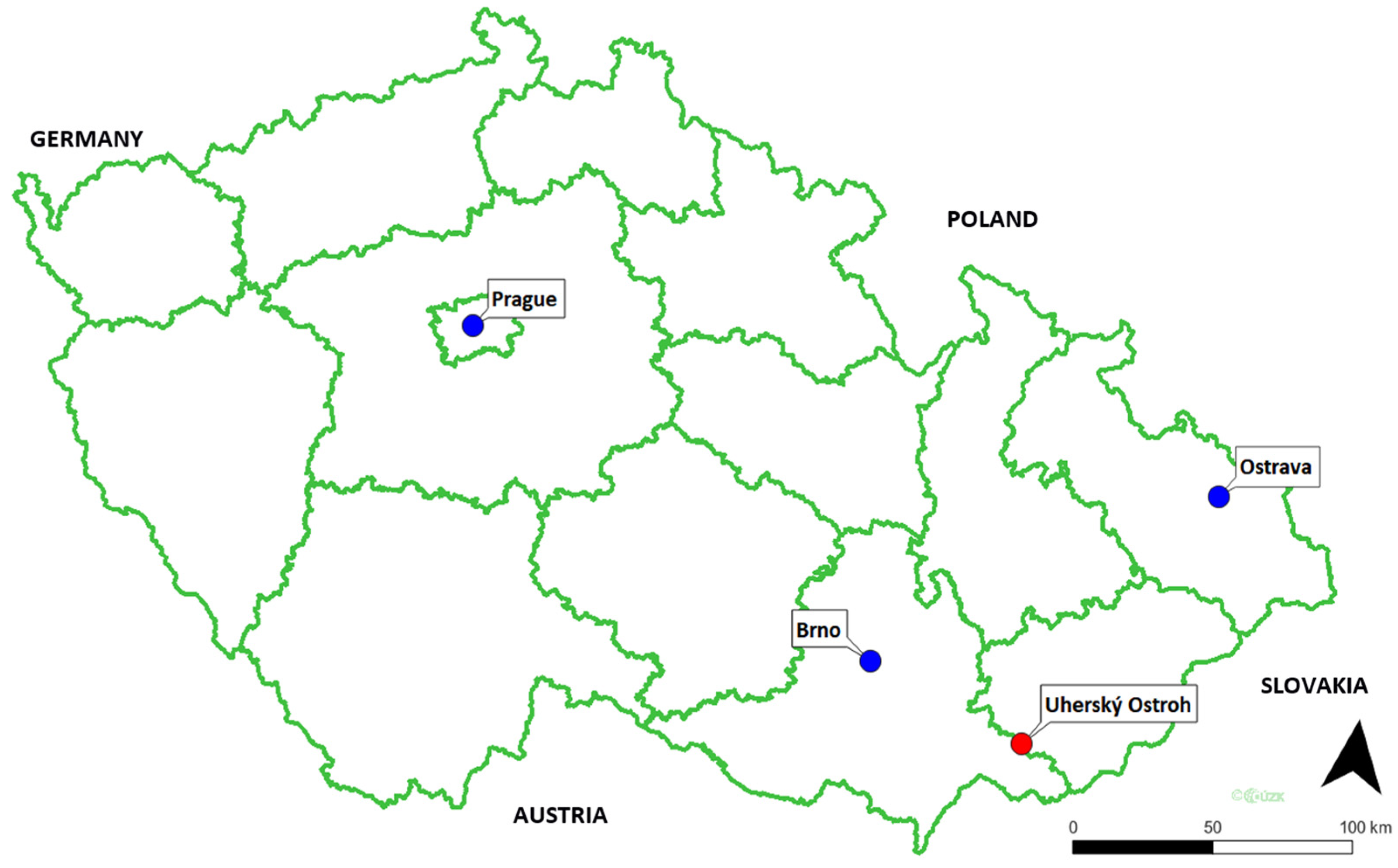
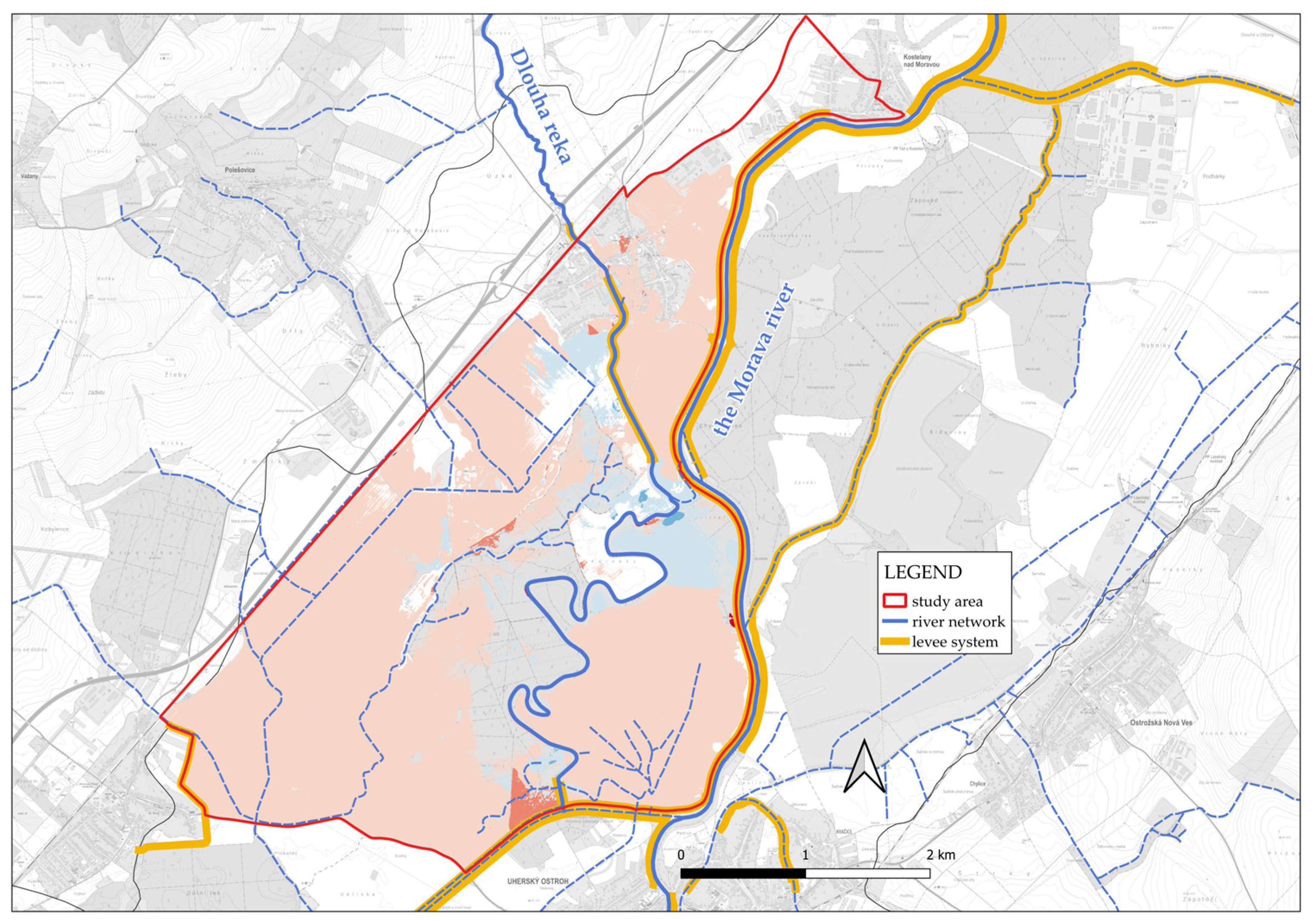
An inundation area on the right bank of the Morava River near the city of Uhersky Ostroh in the Czech Republic was selected for the analysis (Figure 1). This site was chosen due to its representative hydraulic characteristics and varied topography, as well as the availability of high-quality validation data, which enabled calibration of the global model (Section 2.2). The study area encompasses the right-bank Morava River floodplain behind the principal levees. The area is supplied by the local Dlouha Reka stream, approaching the flow domain from the north (Figure 2). Hence, the flood scenarios (Table 1) are related to this local stream. The area is covered mainly by forests, meadows, and agricultural land, with several small drainage trenches, as well as ancient and newly built modern levee structures. The trenches serve mainly for passing smaller floods through the inundation area without the overbanking and flooding of arable land.

4. Analysis, Results, and Discussion

4.1. Comparison of DTMs

Firstly, the DTMs were validated using geodetically surveyed points (GSPs), with three categories of points with respect to surface cover. Most comparisons (2844) were carried out at levee axes and levee slopes covered by mown herbaceous vegetation without trees. Eighteen points were located on solid open surfaces, primarily asphalt and concrete roads; 114 GSPs were situated along levee axes, which were partially shaded by the branches of deciduous trees. The numbers of reference points, the minimum (min_ΔZ) and maximum (max_ΔZ) differences, the systematic error C_H, and the total mean square error RMSE are shown in

Table 2. Evaluation accuracy of DTMs at geodetically surveyed points.

Surface Type	Data Source	No. of Points	min_ΔZ [m]	max_ΔZ [m]	CH [m]	RMSE [m]
Levees without trees	DTM4G	2844	−1.012	0.276	−0.184	0.255
	DTM5G	2844	−0.910	0.352	0.029	0.103
	DTM CG	2844	−0.163	0.314	0.048	0.062
Solid open surface	DTM4G	18	−0.307	−0.013	−0.109	0.132
	DTM5G	18	−0.300	0.026	−0.119	0.144
	DTM CG	18	−0.003	0.045	0.020	0.024
Levees partially shaded by trees	DTM4G	114	−0.325	0.042	−0.130	0.153
	DTM5G	114	−0.296	0.086	−0.047	0.028
	DTM CG	114	−0.033	0.136	0.051	0.055

.

From Table 2, it can be seen that the highest positive difference (approximately 0.35 m) was identified on levees without trees. In general, the overall max_ΔZ of individual DTMs on a given type of surface was comparable, in the range of single decimetres. Simultaneously, the smallest differences were identified when comparing the purpose-built DTMCG with DTM4G and DTM5G. The comparison of the DTMs’ precision with GSPs should consider several factors, such as the time span between LiDAR data acquisition for DTM4G (2013) and the improved DTM5G (2016), both during the vegetation season. DTMCG was prepared from LiDAR data scanned in early spring 2025, before the beginning of the vegetation season. This can partially explain the very low minimum difference between “levees partially shaded by trees” and “levees without trees” for DTMCG because of the absence of leaves on trees and dry herbs at that time. The time of the GSPs’ measurement can also play an important role in the differences between the GSPs and DTMs; as such, the differences between the DTMs and GSPs of all categories with respect to the year of GSP origin were analysed. The GSPs for the “levees without trees” category were surveyed as follows: year 2014—52 GSPs, 2015—521 GSPs, 2016—387 GSPs, 2020—90 GSPs, 2023—1132 GSPs, and 2025—662 GSPs. The results showed that the year of GSP acquisition did not affect the differences between the DTMs and GSPs.

“Solid open surfaces” (mostly streets and parking places) typically do not change height unless the places undergo reconstruction, and these were excluded from this data category using visual retrospective analysis of orthophotos. There were 2 GSPs in 2016, 10 in 2023, and 6 in 2025. The results showed a stable performance of the differences between the DTMCG and GSPs in all years.

Most of the GSPs were measured in 2023 (2001 pts). The remaining GSPs were from 2014 to 2016, except for 18 GSPs on “solid open surfaces” (synchronised with LIDAR scanning in 2025). Certain differences may have resulted from the different site situations during LiDAR data acquisition in 2016 and 2025. The GSPs on “levees partially shaded by trees” (114) were all collected in 2023.

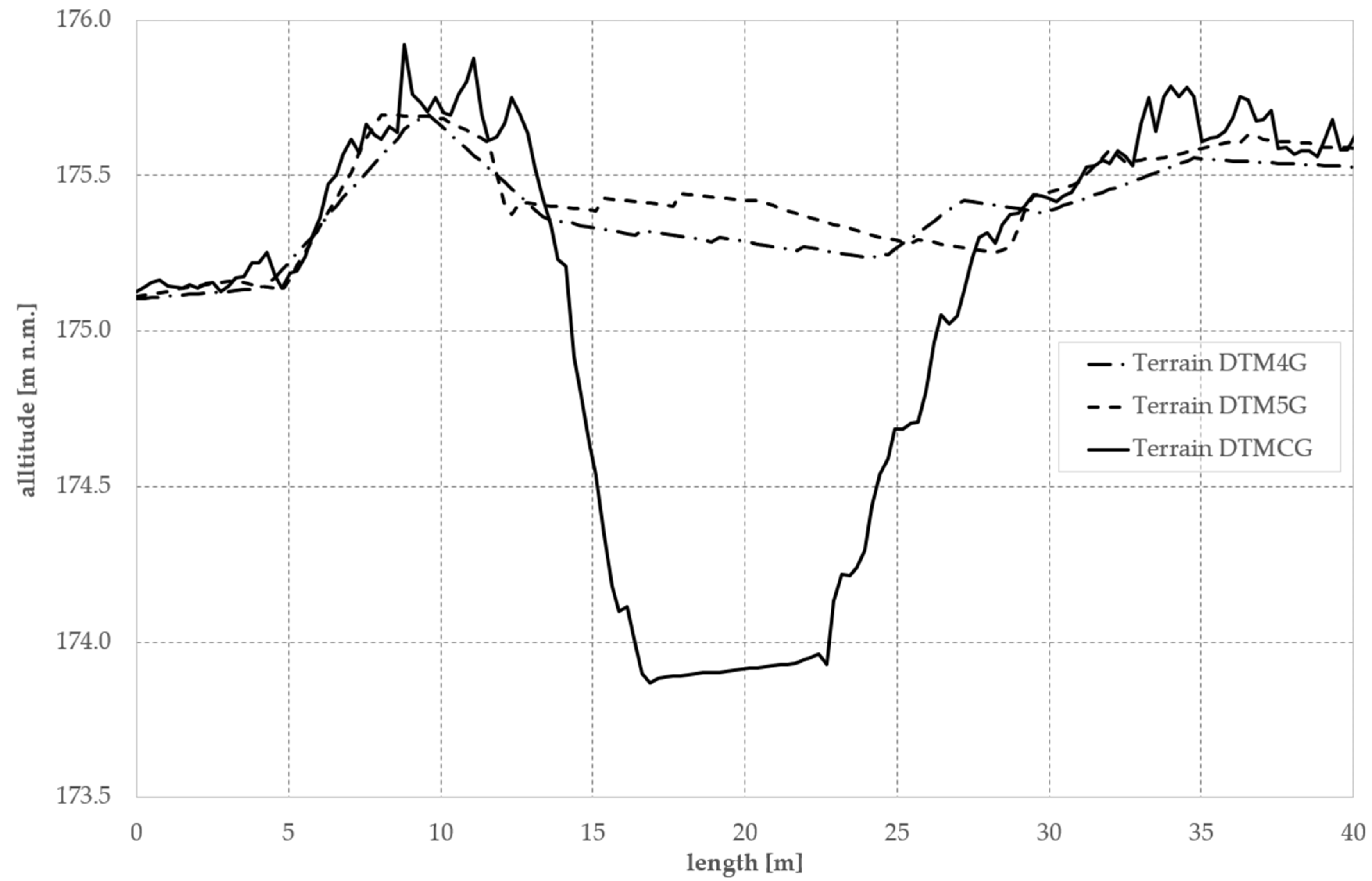
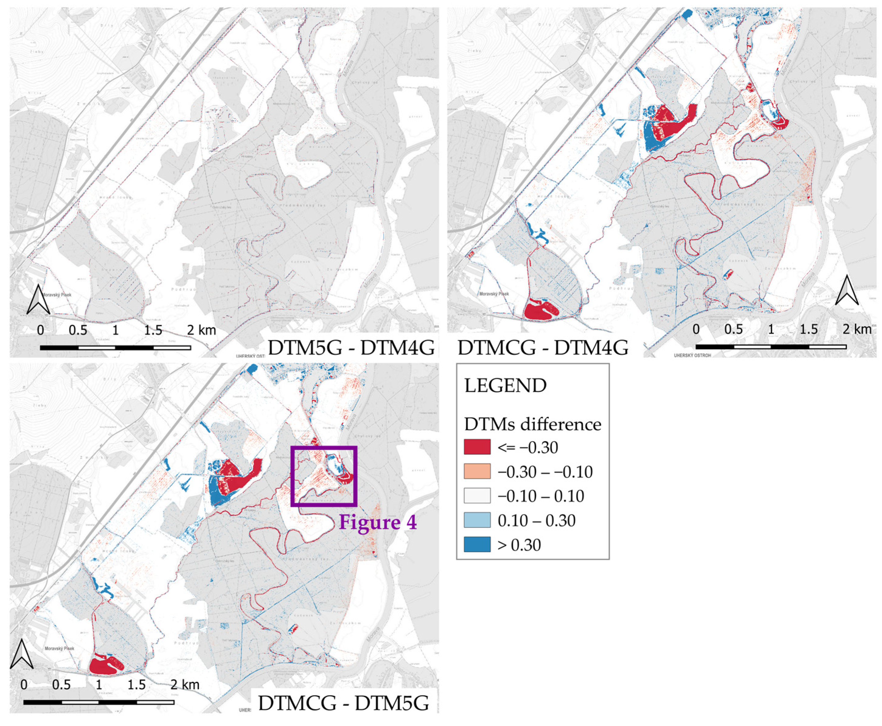
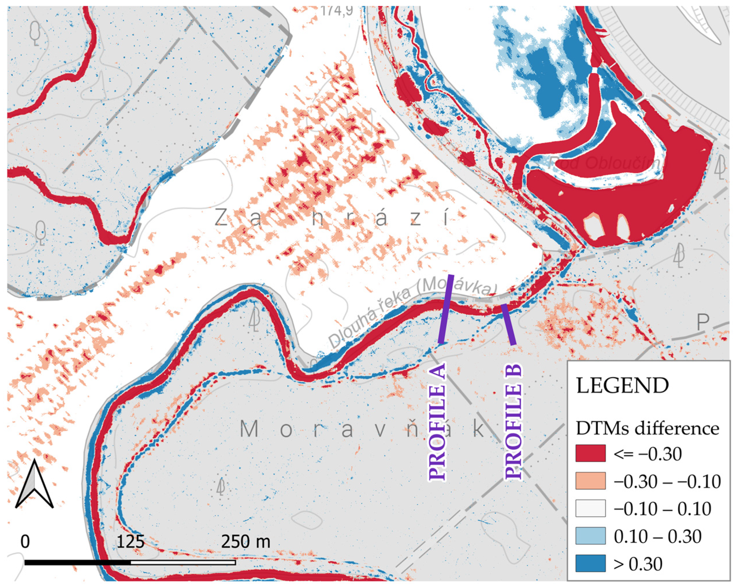
The second step involved comparing the spatial differences between individual DTMs. Figure 3 shows the map with the differences between the altitudes provided by individual DTMs. There was no significant difference between the DTM5G and DTM4G models. However, more significant differences were observed when comparing the models with DTMCG (the details of the selected area are depicted in Figure 4). This indicates improved accuracy when using DTMCG regarding “small-size” terrain bodies, such as small watercourses and historical levee lines (Figure 5). This can play a role when flood discharges pass through the area. Figure 3 and Figure 4 exhibit human activities, and more significant local excavations are depicted by continuous red and blue colours. The colour dots dispersed in wider areas are attributed to the inaccuracy of the older models. The maximum and minimum differences in the DTMs are summarised in Section 4.2, together with the differences in corresponding water levels.

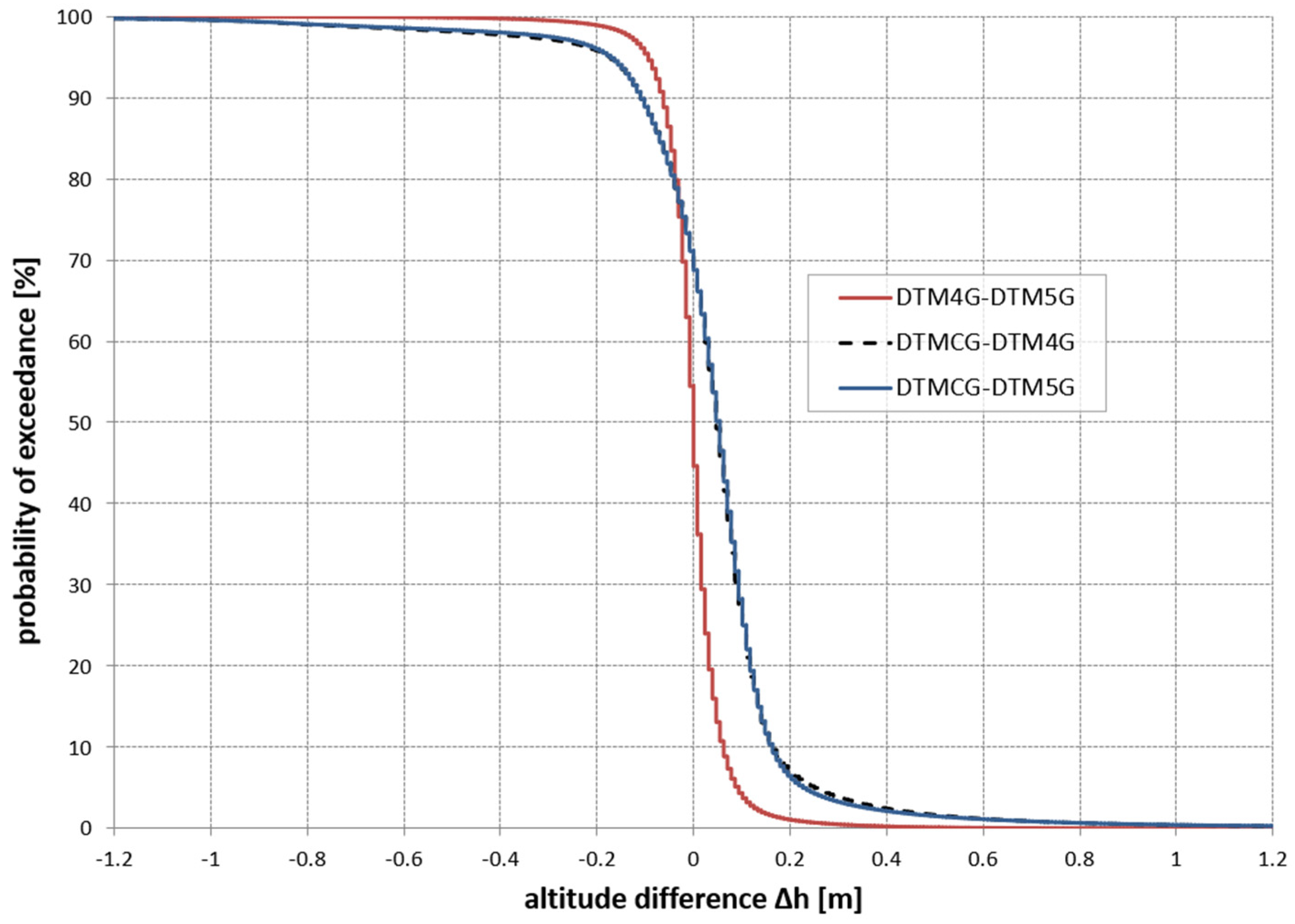
Figure 6 shows the global exceedance (across the entire domain) of the altitude differences between the compared Digital Terrain Models, based on the differences calculated within the model domain extent. In agreement with Figure 3 and Figure 5, DTM4G and DTM5G exhibited minor differences, with more significant differences between these models and DTMCG. Positive differences (DTMCG provides higher altitudes) prevailed (approximately 70%). Both DTM4G and DTM5G were built for the whole territory of the Czech Republic. Their validation points were selected with representativeness criteria for the whole country, and the DTMs were adjusted accordingly between 2014 and 2016. DTMCG reflects the most recent situation, on levees as well as throughout the study domain, and GSPs were collected only there.

Higher differences, both positive and negative, with a very small frequency (a single per cent) occurred in singularities, such as open channels (Figure 6), and in locations subject to human activities in the area, such as gravel pits or fills (Figure 3 and Figure 4).

4.2. Comparison of Hydraulic Modelling Results

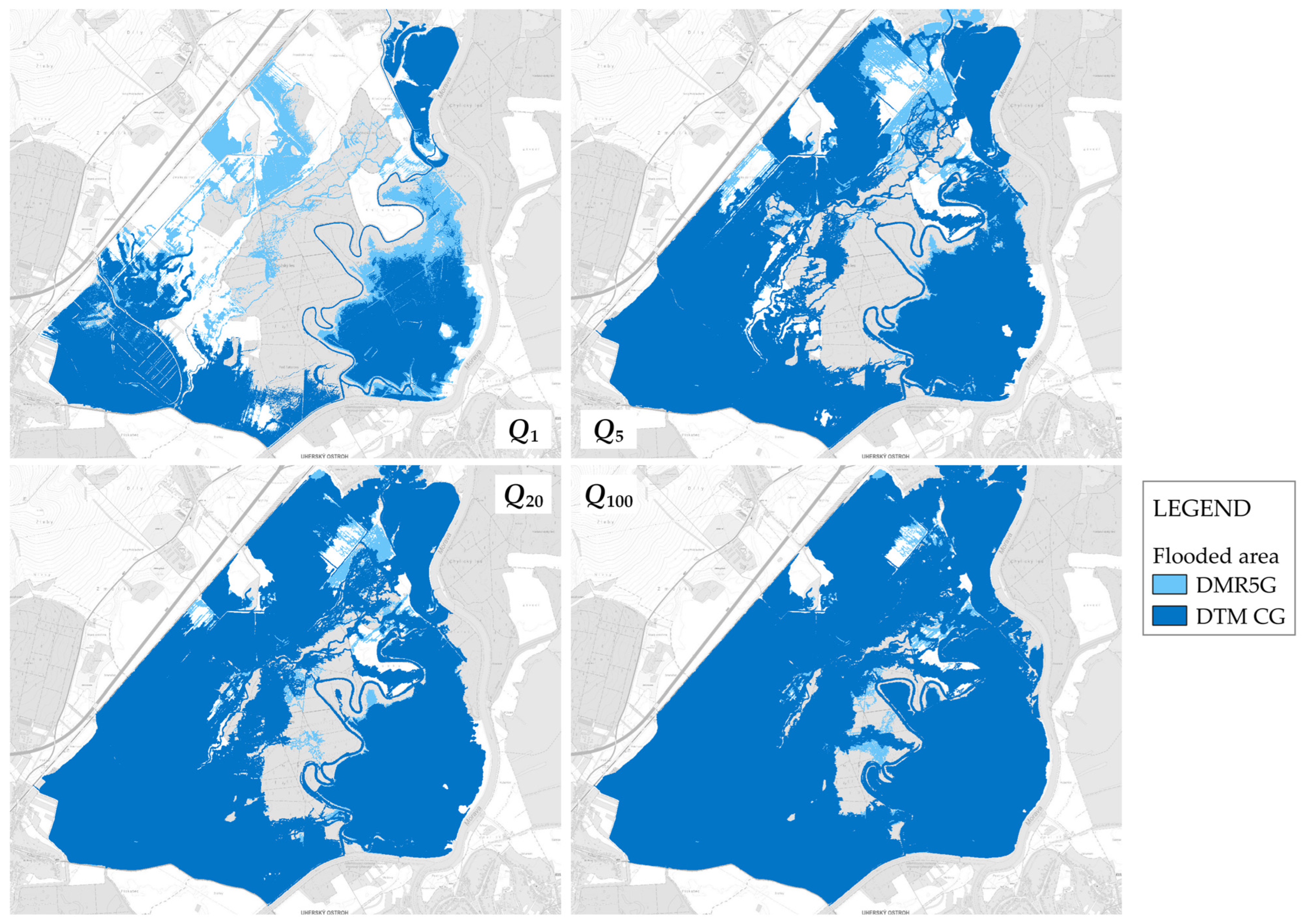
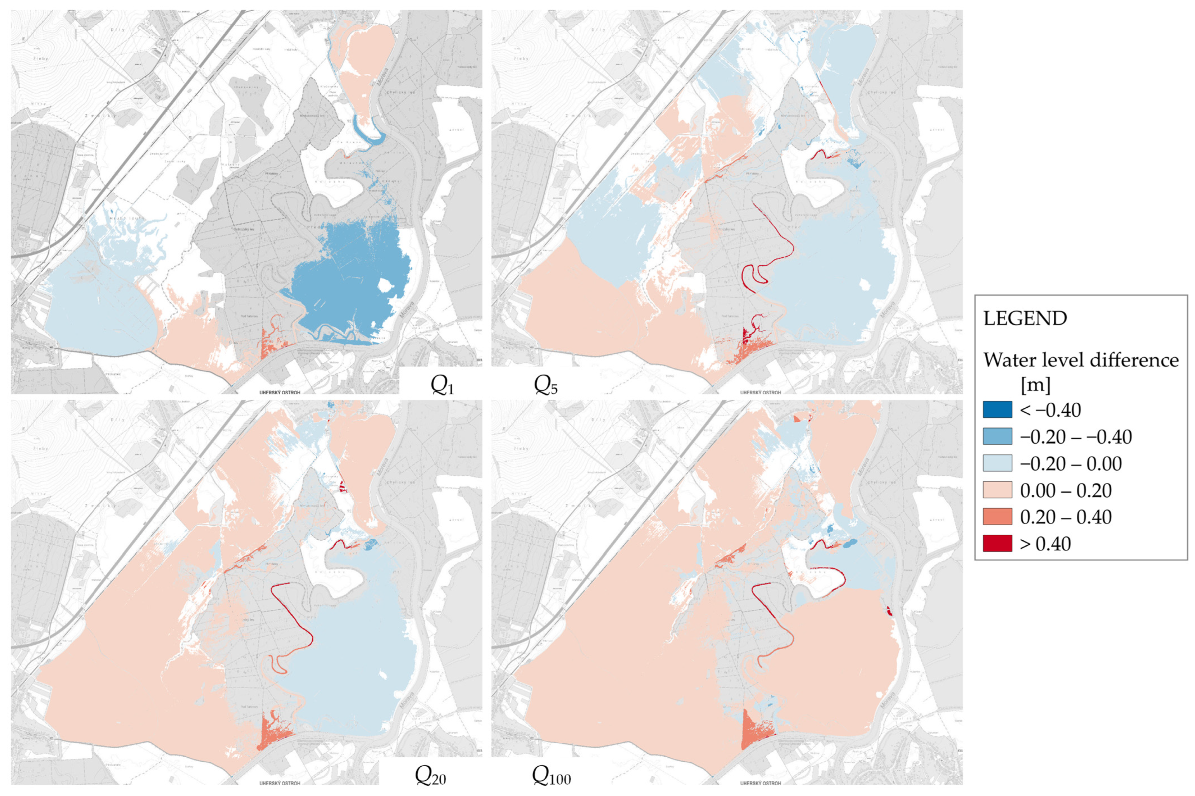
The hydraulic modelling results for the flood scenarios were compared, focusing on the extent of the inundated area and water level altitudes. The comparison of DTM4G and DTM5G indicated only minor differences between these global models (Figure 3); furthermore, hydraulic analysis indicated only minor differences in the water levels obtained for these DTMs. Therefore, for better illustration, the extent of the inundation was compared via flood maps only for the differences between DTM5G and DTMCG (Figure 7).

Table 3. Flooded areas and corresponding differences between flooded areas.

	Flooded Area/Difference in Flooded Area [m2]
	Q1	Q5	Q20	Q100
ADTM4G	6,879,830	8,646,124	10,014,045	11,792,796
ADTM5G	6,128,987	8,159,452	9,523,307	11,657,731
ADTMCG	4,501,616	7,625,233	9,427,562	11,767,930
∆A4-5	750,843	486,672	490,738	135,065
∆ACG-4	−2,378,214	−1,020,891	−586,483	−24,866
∆ACG-5	−1,627,371	−534,219	−95,745	110,199

shows the flooded areas resulting from the individual DTMs. Figure 7 and Table 3 show that using a less accurate DTM resulted in larger flooded areas due to the poor description of the narrow open channels (see also Figure 5), limiting their discharge capacity. These inaccuracies from using DTMs became less significant with increasing flood discharges when most of the area is subject to flooding. Both Figure 7 and Table 3 indicate a significantly smaller flooded area for smaller discharges (Q₁ and Q₅) when using a more detailed DTMCG reflecting local canals (Figure 5). Thus, in the case of DTMCG, smaller floods in the hydraulic model passed mostly through local canals without more extensive overbanking (Figure 7). Local canals played a less significant role in more extensive floods, and the modelling results indicated smaller differences between the individual DTMs. The differences between flooded areas generally decreased with an increasing return period, indicating that the differences in the DTMs were less significant for the results of hydraulic calculations.

The differences in water levels ΔH in the flooded areas are compared in

Table 4. Evaluation of DMT and water level differences.

Flood Scenario	Differences	min_ΔZ [m]	max_ΔZ [m]	min_ΔH [m]	max_ΔH [m]	MAE [m]
Q1	∆Z4-5; ∆H4-5	−0.742	1.117	−0.251	0.299	0.057
	∆ZCG-4; ∆HCG-4	−2.109	1.711	−0.383	0.585	0.183
	∆ZCG-5; ∆HCG-5	−2.336	1.984	−0.467	0.752	0.191
Q5	∆Z4-5; ∆H4-5	−1.891	1.117	−0.095	0.281	0.050
	∆ZCG-4; ∆HCG-4	−2.578	1.648	−0.216	0.364	0.119
	∆ZCG-5; ∆HCG-5	−2.547	1.484	−0.163	0.319	0.117
Q20	∆Z4-5; ∆H4-5	−1.891	1.117	−0.143	0.146	0.059
	∆ZCG-4; ∆HCG-4	−2.938	1.648	−0.215	0.343	0.105
	∆ZCG-5; ∆HCG-5	−2.930	1.625	−0.159	0.305	0.105
Q100	∆Z4-5; ∆H4-5	−1.891	2.031	−0.109	0.109	0.047
	∆ZCG-4; ∆HCG-4	−2.984	1.813	−0.196	0.330	0.101
	∆ZCG-5; ∆HCG-5	−3.797	1.969	−0.117	0.297	0.096

. Figure 8 shows the differences in water levels, comparing the results using DTM5G and DTMCG. The red zones (higher negative differences) appear upstream from obstructions, which influence hydraulics upstream from the singularity (backwaters). Red zones also correspond to small water courses, which are discontinuous in the case of DTM5G and, thus, conduct only a minor amount of water with a lower water level.

Table 4 and Figure 8 show that both positive and negative differences ∆H between the more accurate DTMCG and the older DTM4G and DTM5G drop with increasing flood discharge. Table 4 shows higher differences in water levels exceeding 0.75 m in cases of “smaller” discharges, such as Q₁. These differences are attributed to the differences in the DTMs at elongated singularities in areas such as local canals or field roads. These comparisons revealed the impact of channels and roads in DTMCG that were not identified in DTM5G and DTM4G. The older DTMs did not represent the local terrain elevations or depressions as accurately as the more advanced DTMCG. In cases of higher discharges, Q₂₀ and Q₁₀₀, the modelled water levels were locally higher for DTMCG by less than +0.35 m.

The analysis of the local impact of differences ∆Z in the DTMs on local differences in water level ∆H indicated that the variation in ∆H (dependent variable) is not simply predictable using ∆Z (independent variable).

The analysis of mean absolute error (MAE) showed that the less accurate DMT4G and DMT5G provided a smaller mutual difference ΔH_4-5. For the more accurate DMTCG, the differences ΔH_CG-4 and ΔH_CG-5 decreased from approximately MAE = 0.191 m for the discharge Q₁ to MAE = 0.101 for the discharge Q₁₀₀.

However, hydraulic modelling of variants is necessary for a rigorous analysis, as demonstrated in this study. Differences ∆Z between individual DTMs may have influenced differences in water level ∆H beyond the corresponding location. Differences ∆Z (changes in the level of obstruction and canal bottom) dominantly affected the water level upstream from the singularity via the backwater rate in the case of the higher DTM level and via the lower water level in the case of the continuous canal (see Figure 5).

The study results (Figure 8) show that in a more rugged topography containing “narrow” linear elevations, such as levees, roads, and railroads, the local inaccuracies in the DTM would result in higher errors in the achieved flooded area and water levels. A more detailed DTMCG should be used in these cases. However, more studies in different floodplains are needed for rigorous generalisation.

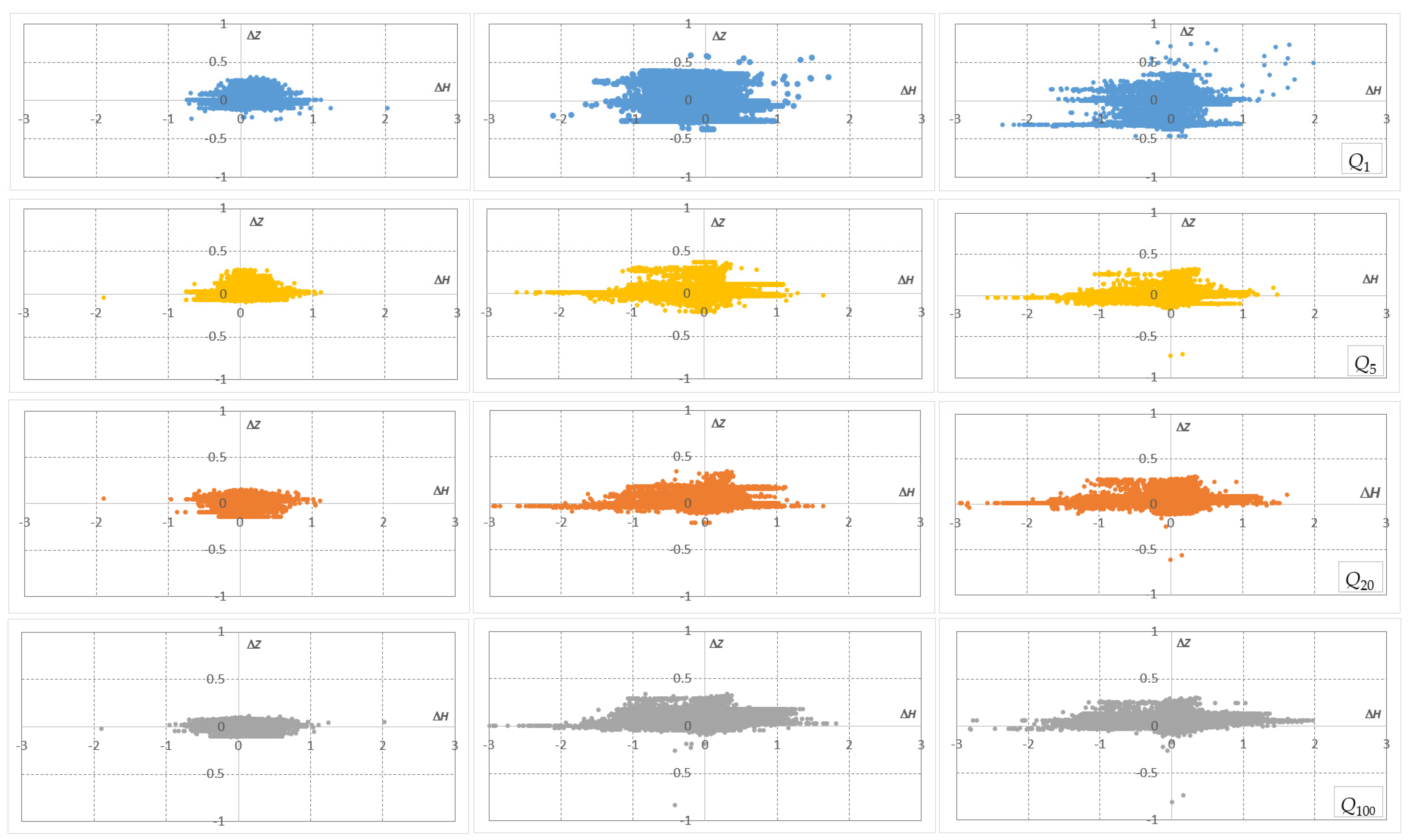
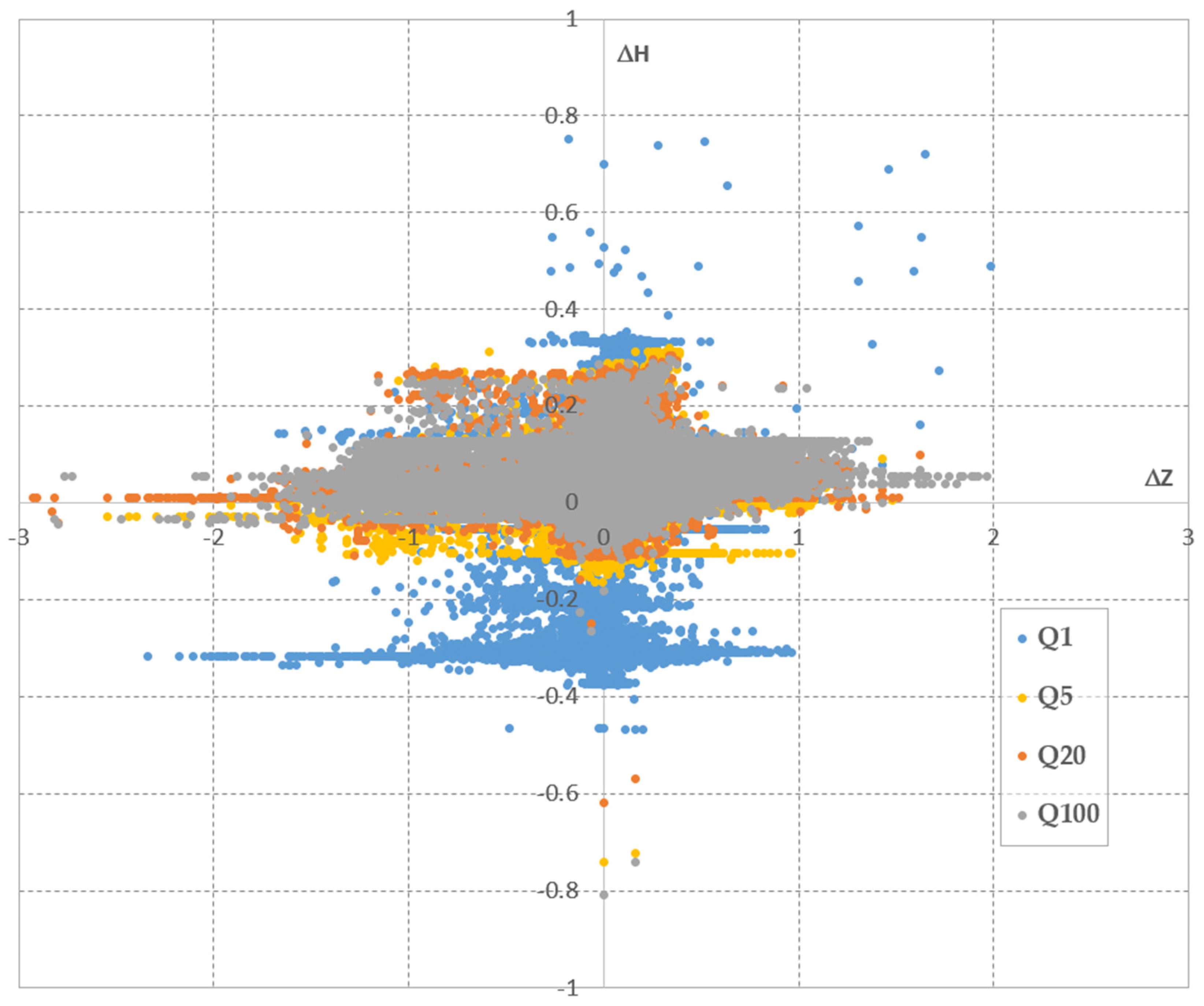
The overall impact of the DTMs on the resulting water levels was graphically assessed via the differences ∆Z corresponding to ∆H. Figure 9 and Figure 10 show the “agreement” between the ∆Z and ∆H values for individual pixels in the modelled flow domain. The results for DTM4G and DTM5G are relatively similar. The values appear more dispersed at low flows compared with DTMCG. For higher flows, ∆H decreases for the same ∆Z value.

Figure 9 and Figure 10 show a very poor correlation between the ∆Z and ∆H values. The physical explanation is that local DTM differences usually hydraulically propagate into a larger area upstream of the singularity, even if the differences between DTMs in this backwater area can be quite small.

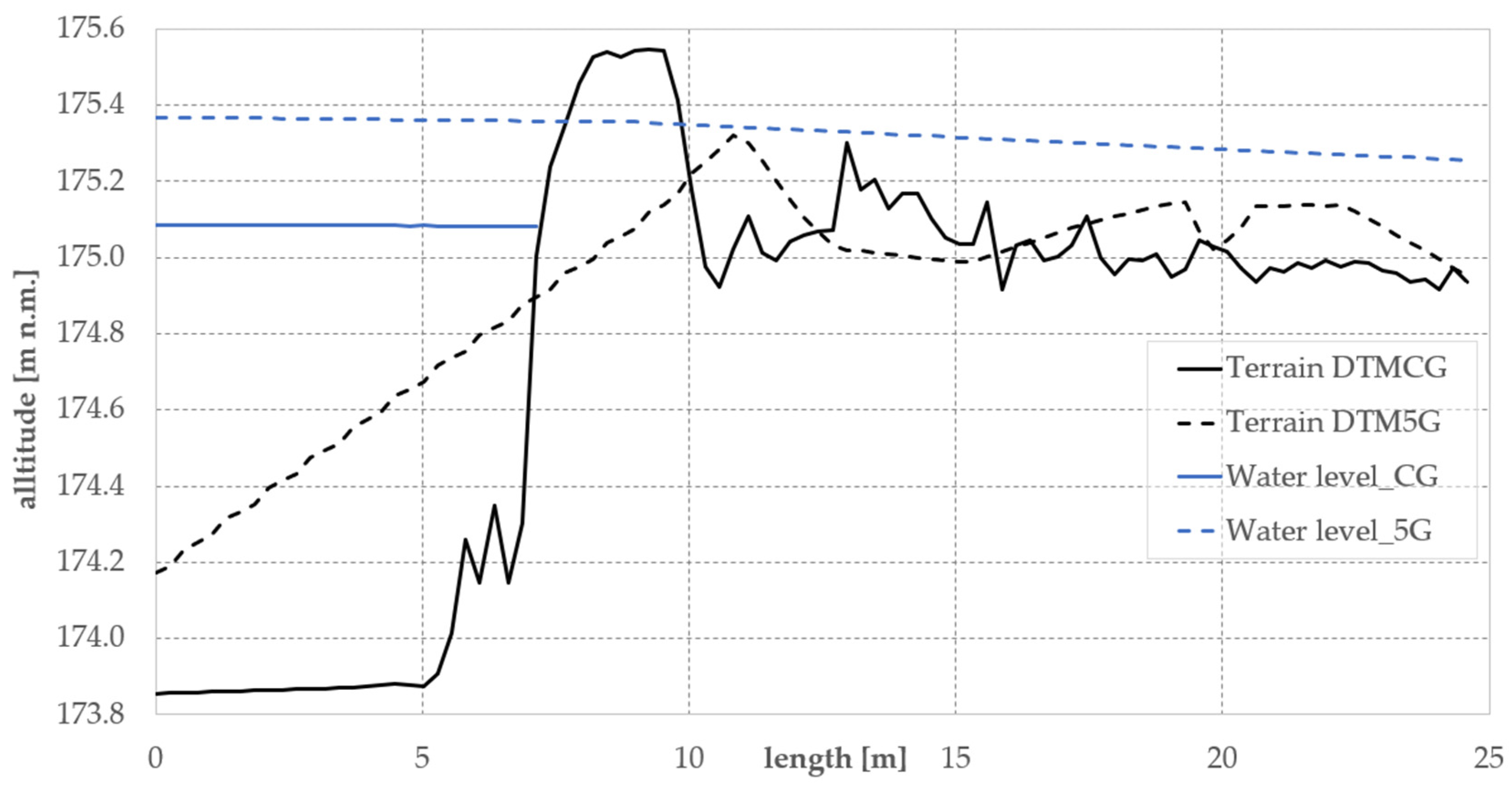
Figure 11 illustrates the details of cross-section B (see Figure 4), showing local differences in DTM5G and DTMCG and the corresponding water levels obtained with the hydraulic model. The lower water level for DTMCG corresponds to a more accurately represented open canal with higher capacity; meanwhile, the water level calculated using DTM5G, with a poorly defined levee and canal, indicates overbanking. As the terrain surface defines the geometry influencing water flow, even small differences in elevation or the representation of local features can lead to substantial variations in simulated water levels, flow patterns, and the inundation extent upstream from the locality. The comparison between DTM5G and the higher-precision DTMCG in Profile B illustrates these issues (Figure 11).

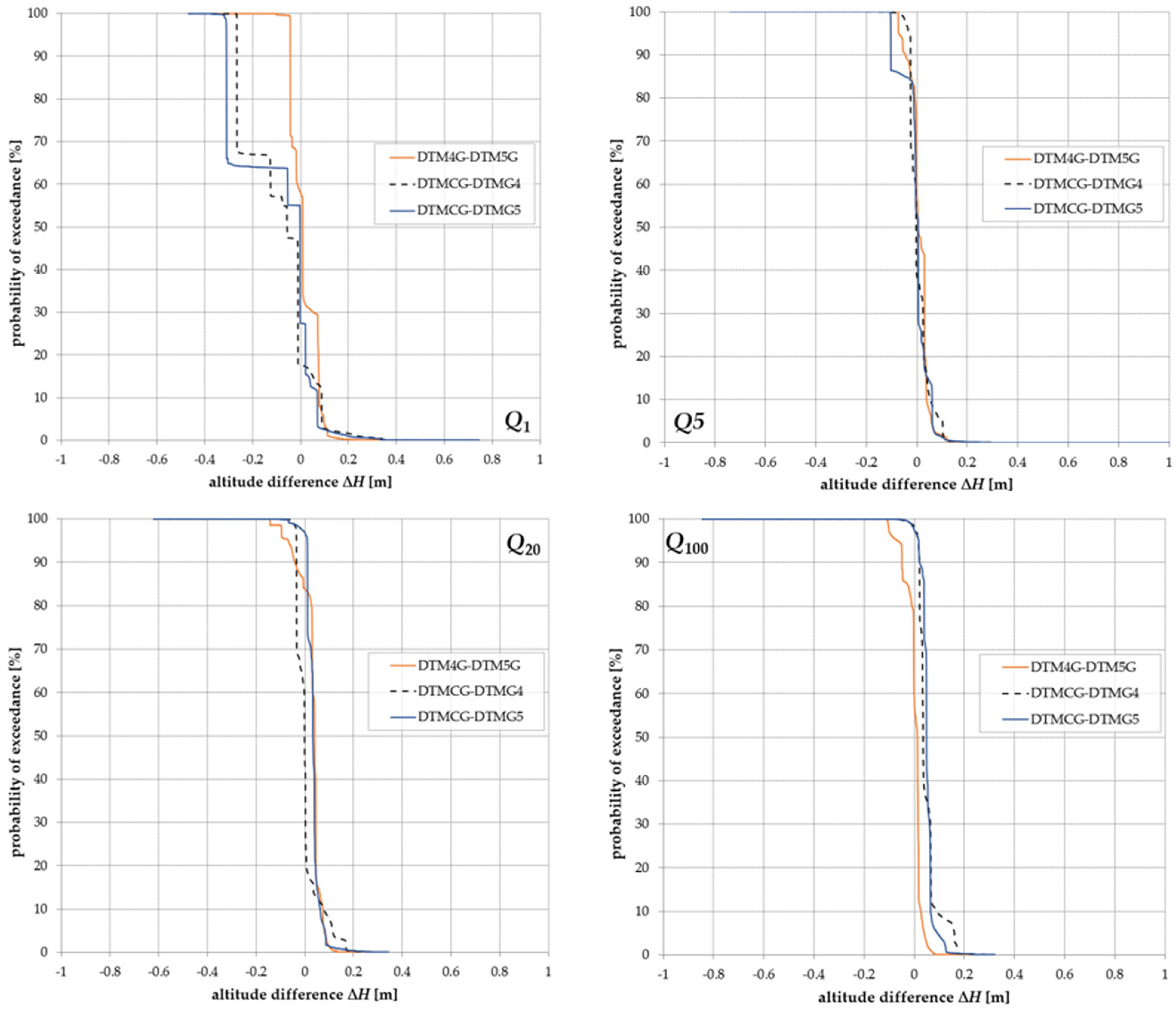
Figure 12 shows the exceedance of the water level differences obtained via hydraulic modelling for four flood scenarios using various Digital Terrain Models. In agreement with Figure 7, Figure 8, Figure 9 and Figure 10, small differences were obtained when using DTM4G and DTM5G. The more significant differences between the results using these models and DTMCG can be attributed to the higher accuracy of the DTMCG.

Meanwhile, larger and more frequent differences were observed in the case of the Q₁ scenario, where the maximum difference of approximately 0.75 m (see Table 4) occurred as a single value, with an empirical exceedance probability lower than 0.001. Negative differences from −0.25 to −0.30 m were more frequent in the Q1 scenario, accounting for an exceedance of approximately 65%. This can be attributed to the higher water level obtained using the less-accurate DTM4G and DTM5G, with poor information about local water courses. Positive values were interpreted as backwater due to locally elevated terrain.

For higher flood discharges from Q5 to Q100, the differences were generally reduced to a value of ~0.1 m, accounting for less than approximately 10% of all values.

A key challenge is that hydraulic models respond to terrain errors in a non-local and nonlinear way. A small rise in the terrain (e.g., a smoothed levee or missing channel) can influence the backwater effect upstream, increase water levels over a large area, alter the flow direction and velocity fields, or “artificially” enlarge the inundation extent. Conversely, a missing levee or depression may cause changes in drainage or underestimated water levels. This explains the lack of a direct correlation between ΔZ and ΔH. A small elevation error in a hydraulically sensitive area can have a much larger impact than a large elevation error in a flat, already inundated floodplain.

5. Conclusions

In this paper, the impact of DTM accuracy on the results of 2D hydraulic flood modelling was analysed. Knowledge about possible inaccuracies is important for flood routing management, the specification of flooded areas, and the design of setback levees located at the edge of the floodplain.

Three DTMs were tested and compared: the fourth- and fifth-generation DTMs and the purpose-built DTMCG developed by the CzechGlobe institute, CAS. Hydraulic modelling was carried out for flood discharges with return periods of 1, 5, 20, and 100 years, and an inundation area on the right bank of the Morava River was chosen for the analysis. The following findings and conclusions can be derived from the analysis:

• There is no direct correlation between the inaccuracy of DTMs and errors in water levels obtained via hydraulic modelling.
• The differences in water levels obtained via hydraulic modelling (due to DTM inaccuracy) reduce with increasing flood discharge.
• Minor DTM differences manifesting in local terrain rises can obstruct the flow in the hydraulic model, influence the backwater upstream, and increase water levels over a large area. Conversely, a missing levee or depression in a less-accurate DTM may cause an underestimation of water levels in areas with a reasonable fit between DTMs.
• The error in the calculated water level exceeded 0.75 m for Q₁ and approximately 0.33 m for Q₁₀₀. This error should not be generalised and depends on the morphology and segmentation of the floodplain, the configuration of the hydraulic model, local changes and human interventions in the area, and the DTMs used, as well as their accuracy and resolution.
• The higher point cloud density when using DTMCG is associated with approximately double computational cost during pre-processing, specifically in TIN and raster generation (compared to DTM4G and DTM5G data), which should be considered in large-scale applications.

The authors’ experience indicates that, for more general flood routing studies, less accurate DTMs—such as DTM4G and DTM5G—may be applied, considering the expected error deriving from their inaccuracy and poor resolution. For detailed flood protection studies, higher-accuracy DTMs are recommended. If a less-accurate DTM is used for a detailed analysis, a comprehensive and extensive site investigation, geodetic measurements, and “manual” improvement of the DTM at the singularities are necessary.

References

1. European Parliament and Council. Directive 2007/60/EC of the European Parliament and of the Council of 23 October 2007 on the Assessment and Management of Flood Risks. Official Journal of the European Union, L 288, pp. 27–34. Available online: https://eur-lex.europa.eu/eli/dir/2007/60/oj (accessed on 25 May 2026).
2. European Commission. Biodiversity Strategy 2030: Barrier Removal for River Restoration. 2021. Publications Office of the European Union. Available online: https://op.europa.eu/en/publication-detail/-/publication/0146a7ba-2f20-11ed-975d-01aa75ed71a1 (accessed on 25 May 2026).
3. Casas, A.; Benito, G.; Thorndycraft, V.R.; Rico, M. The topographic data source of digital terrain models as a key element in the accuracy of hydraulic flood modelling. Earth Surf. Process. Landf. 2006, 31, 444–456. [Google Scholar] [CrossRef]
4. Alho, P.; Hyyppä, H.; Hyyppä, J. Consequence of DTM Precision for Flood Hazard Mapping: A Case Study in SW Finland. Nord. J. Surv. Real Estate Res. 2009, 6, 21–39. [Google Scholar]
5. Horritt, M.S.; Bates, P.D. Evaluation of 1D and 2D numerical models for predicting river flood inundation. J. Hydrol. 2002, 268, 87–99. [Google Scholar] [CrossRef]
6. Shen, D.; Wang, J.; Cheng, X.; Rui, Y.; Ye, S. Integration of 2-D hydraulic model and high-resolution lidar-derived DEM for floodplain flow modeling. Hydrol. Earth Syst. Sci. 2015, 19, 3605–3616. [Google Scholar] [CrossRef]
7. Bures, L.; Roub, R.; Sychova, P.; Gdulova, K.; Doubalova, J. Comparison of bathymetric data sources used in hydraulic modelling of floods. J. Flood Risk Manag. 2018, 12, e12495. [Google Scholar] [CrossRef]
8. Luppichini, M.; Favalli, M.; Isola, I.; Nannipieri, L.; Giannecchini, R.; Bini, M. Influence of Topographic Resolution and Accuracy on Hydraulic Channel Flow Simulations: Case Study of the Versilia River (Italy). Remote Sens. 2019, 11, 1630. [Google Scholar] [CrossRef]
9. Sanders, B.F. Evaluation of on-line DEMs for flood inundation modeling. Adv. Water Resour. 2007, 30, 1831–1843. [Google Scholar] [CrossRef]
10. Xu, K.; Fang, J.; Fang, Y.; Sun, Q.; Wu, C.; Liu, M. The Importance of Digital Elevation Model Selection in Flood Simulation and a Proposed Method to Reduce DEM Errors: A Case Study in Shanghai. Int. J. Disaster Risk Sci. 2021, 12, 890–902. [Google Scholar] [CrossRef]
11. Al-Ghosoun, A.; El Moçayd, N.; Seaid, M. A surrogate model for efficient quantification of uncertainties in multilayer shallow water flows. Environ. Model. Softw. 2021, 144, 105176. [Google Scholar] [CrossRef]
12. Malekhosseini, S.H.; Khorshidi, H.; Szymkiewicz, R. Uncertainty analysis of simplified 1D and 2D shallow water equations via the Karhunen–Loéve expansion and Monte Carlo simulations. Stoch. Environ. Res. Risk Assess. 2023, 38, 1051–1070. [Google Scholar] [CrossRef]
13. Machado, G.L. Numerical Simulation of Uncertainty Quantification for Shallow Water Models. Bachelor’s Thesis, Rijksuniversiteit Groningen, Groningen, The Netherlands, 2025. [Google Scholar]
14. Reutebuch, S.E.; McGaughey, R.J.; Andersen, H.E.; Carson, W.W. Accuracy of a high-resolution lidar terrain model under a conifer forest canopy. Can. J. Remote Sens. 2003, 29, 527–535. [Google Scholar] [CrossRef]
15. Müller, J.; Gärtner-Roer, I.; Thee, P.; Ginzler, C. Accuracy assessment of airborne photogrammetrically derived high-resolution digital elevation models in a high mountain environment. ISPRS J. Photogramm. Remote Sens. 2014, 98, 58–69. [Google Scholar] [CrossRef]
16. Höhle, J.; Höhle, M. Accuracy assessment of digital elevation models by means of robust statistical methods. ISPRS J. Photogramm. Remote Sens. 2009, 64, 398–406. [Google Scholar] [CrossRef]
17. Garrote, J. Free Global DEMs and Flood Modelling—A Comparison Analysis for the January 2015 Flooding Event in Mocuba City (Mozambique). Water 2022, 14, 176. [Google Scholar] [CrossRef]
18. Javas, J.; Roesbianto, A.S.B.; Sihombing, Y.I.; Farid, M.; Adityawan, M.B.; Kuntoro, A.A.; Suwarman, R.; Yosa, I.M. Open-access digital elevation model (DEM) selection for flood inundation modelling using HEC-RAS in Capital City of Nusantara. IOP Conf. Ser. Earth Environ. Sci. 2024, 1343, 012036. [Google Scholar] [CrossRef]
19. Caletka, M. Možnosti extrapolace digitálního modelu terénu z rastru DMR 5G [Possibilities of extrapolation of a digital terrain model from the DMR 5G grid]. Vodohospod. Tech.-Ekon. Inf. 2017, 59, 18–23. [Google Scholar]
20. Sidek, L.M.; Jaafar, A.S.; Majid, W.H.A.W.A.; Basri, H.; Marufuzzaman, M.; Fared, M.M.; Moon, W.C. High-Resolution Hydrological-Hydraulic Modeling of Urban Floods Using InfoWorks ICM. Sustainability 2021, 13, 10259. [Google Scholar] [CrossRef]
21. He, J.; Zhang, S.; Cui, X.; Feng, W. Remote sensing for shallow bathymetry: A systematic review. Earth-Sci. Rev. 2024, 258, 104957. [Google Scholar] [CrossRef]
22. Tompalski, P.; Coops, N.C.; White, J.C.; Wulder, M.A.; Yuill, A. Characterizing streams and riparian areas with airborne laser scanning data. Remote Sens. Environ. 2017, 192, 73–86. [Google Scholar] [CrossRef]
23. Ettritch, G.; Hardy, A.; Bojang, L.; Cross, D.; Bunting, P.; Brewer, P. Enhancing digital elevation models for hydraulic modelling using flood frequency detection. Remote Sens. Environ. 2018, 217, 506–522. [Google Scholar] [CrossRef]
24. Čubanová, L.; Rumann, J.; Rutzká, A.; Vidová, A.; Dušička, P. Verification of the Manning’s Roughness Coefficient of Fish Pass Riverbeds Using Drone-Based Photogrammetry. Water 2025, 17, 1409. [Google Scholar] [CrossRef]
25. CUZK. DMR 5G Technical Report; CUZK: Prague, Czech Republic, 2016. [Google Scholar]
26. Knapík, J. Technical Report to the Digital Terrain Models of the 4th and 5th Generation (DTM4G, DTM5G); Land-Surveying Administration: Pardubice, Czech Republic, 2025.
27. Delaunay, B. Sur la Sphère Vide. A la Mémoire de Georges Voronoï. Bulletin de l’Académie des Sciences de l’URSS. Classe des Sciences Mathématiques et Naturelles. Leningrad, USSR, 1934, No. 6, pp. 793–800. Available online: http://mi.mathnet.ru/eng/im4937 (accessed on 25 May 2026).
28. Brunner, G.W. HEC-RAS Hydraulic Reference Manual; U.S. Army Corps of Engineers: Washington, DC, USA, 2020.
29. Vreugdenhil, C.B. Numerical Methods for Shallow-Water Flow; Kluwer Academic Publishers: Dordrecht, The Netherlands, 1998. [Google Scholar]
Figure 1. Geolocation of the study area.
Water 18 01312 g001
Figure 2. Study area: right-bank floodplain behind the Morava river levees.
Water 18 01312 g002
Figure 3. Differences in Digital Terrain Models (area of the detail is marked in Figure 4). The national coordinate system EPSG:5514-S-JTSK/Krovak East North was applied.
Water 18 01312 g003
Figure 4. Detail of Figure 3, showing differences between DTMCG and DTM5G. Profiles marked by violet: A depicted in Figure 5; B depicted in Figure 11.
Water 18 01312 g004
Figure 5. The terrain corresponding to considered DTMs: profile A across a small stream.
Water 18 01312 g005
Figure 6. Exceedance curves of differences ∆Z between DTMs.
Water 18 01312 g006
Figure 7. Extent of flooded area compared for Q1, Q5, Q20, and Q100 using DTM5G and DTMCG.
Water 18 01312 g007
Figure 8. Differences ∆HCG-5 in water levels.
Water 18 01312 g008
Figure 9. Plots of ΔZ against ΔH. From the left: 4G-5G, CG-4G, and CG-5G.
Water 18 01312 g009
Figure 10. Detailed combined plot of ΔZ against ΔH for all flood scenarios for CG-5G differences.
Water 18 01312 g010
Figure 11. Resulting water level for Q5 in Profile B (location in Figure 4).
Water 18 01312 g011
Figure 12. Empirical exceedance curves of differences in ∆H for individual discharge scenarios.
Water 18 01312 g012