Optimization of Concurrent Seawater and Freshwater Pumping from Coastal Aquifers

Abstract

Covering water demand for secondary uses with resources of inferior quality is already an established practice. In coastal aquifers, saline groundwater can serve as an alternative source. In this paper, we examine concurrent optimization of freshwater and seawater pumping from a coastal aquifer, which may lead to more efficient overall solutions. The particular objective is to determine well locations and pumping rates that meet specified freshwater and saline water demands while preventing seawater intrusion into freshwater wells. A genetic algorithm code is used as an optimization tool, combined with a groundwater flow simulation model based on the Boundary Element Method (BEM). The BEM scheme has a relatively low computational cost and can be efficiently incorporated into the genetic algorithm’s fitness evaluation. Validity of the resulting optimal solutions is further investigated using two, more detailed, groundwater flow and mass transport models: (a) A combination of BEM with a particle-tracking (moving point) technique to simulate seawater movement from the coast towards the wells, and (b) the MODFLOW 6 computational package, including the Groundwater Transport (GWT) model for solute transport. The procedure is illustrated through its application to a synthetic coastal aquifer.

1. Introduction

Water (and energy) resources are basic prerequisites for the development of human activities. Despite scientific progress and technological achievements, water balance evolution is unfavorable in many areas of the world, due to increases in population and per capita water consumption. Moreover, pollution may render water resources useless or expensive. Coastal areas are vulnerable to water deficit problems, particularly those suffering from heavy concentration of human activities. An additional concern is climate change, namely the reduction in precipitation or change in its pattern, leading to both longer dry periods and extreme rain events. In coastal areas, rise in sea surface is also a threat. All these factors render optimal allocation of water to achieve socially fair and financially efficient development very challenging [1].

One way to alleviate water resources management problems is to cover part of the non-potable water demand (e.g., for toilet flushing) with sources of non-potable quality [2]. Furthermore, in coastal areas, especially in arid and semi-arid regions, saline groundwater is increasingly recognized as a strategic non-conventional water resource for irrigation, provided that its use is embedded within appropriate soil–water–crop management practices [3,4,5]. Sustainable use of saline water in irrigation systems depends on the conjunctive management of fresh and saline water resources, crop diversification, and the adoption of salt-tolerant crop varieties—practices that can enhance water use efficiency and support climate-resilient agricultural production in marginal and water-scarce environments [6,7,8].

Concurrent optimization of drinking water and secondary water systems across all stages is very helpful [9]. In coastal aquifers, most previous optimization studies have focused on maximizing freshwater pumping under constraints related to seawater intrusion [10,11], without explicitly and concurrently optimizing saline water abstraction for non-potable uses. Such solutions may have a higher initial cost and require careful planning. Our work addresses this gap by jointly optimizing freshwater and seawater well systems in a coastal aquifer, explicitly accounting for saline water demand as a management target. In a first step, a genetic algorithm (GA) code is used as an optimization tool. It is combined with a groundwater flow simulation model, based on the boundary element method (BEM), to calculate seawater inflow to the coastal aquifer. This model has a relatively low computational cost and is efficiently incorporated into the objective (evaluation) function of genetic algorithms. Then, the optimized solution is further checked, using two, more detailed, groundwater flow and mass transport models: (a) a combination of BEM with a particle-tracking (moving point) technique to simulate seawater movement from the coast towards the wells, and (b) the MODFLOW computational package, including the Groundwater Transport (GWT) model for solute transport. The use of two different computational tools in the final step that serves to underline that choices for any specific case study may vary. The paper mainly aims to emphasize: (a) the importance of concurrent optimization of saltwater and freshwater pumping systems; (b) the advantages of the outlined two-step methodology.

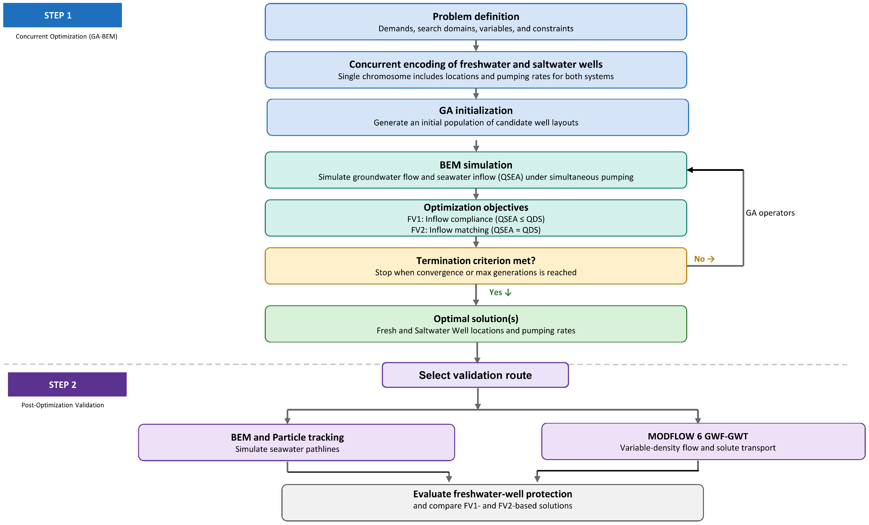
The overall two-step methodology is outlined in Figure 1. The computational tools are briefly described in Section 2, while their combined use is explicitly presented in the application example of Section 3. Conclusions are presented in Section 4.

2. Computational Tools

2.1. Genetic Algorithms

Genetic Algorithms (GAs) are essentially a simplified mathematical imitation of the biological process of species evolution. They are the older sister, if not the mother, of bio-inspired optimization techniques. Initially, they were introduced in 1975 by Holland [12]. They start with several “random” problem solutions, which are called chromosomes and constitute the population of the first generation. Population size (PS) is usually predetermined. In binary genetic algorithms, which are used in this paper, each chromosome is a binary string.

Each chromosome of the first generation undergoes evaluation, by means of a pertinent function or process, which assigns a “fitness value” to it. This process depends entirely on the specific application of genetic algorithms. Then, the second generation is produced, by means of certain operators, which imitate biological processes and apply to the chromosomes of the first generation. The main genetic operators are (a) selection (b) crossover and (c) mutation. Many other operators have also been proposed and used.

Selection is used first. Using the chromosomes’ fitness value results in the construction of the “intermediate” population, to which the remaining operators apply. A detailed description of these operators is out of the scope of this paper. In summary, we mention that in our code the tournament procedure, including an elitist approach, is used in selection. Then, typical one-point crossover and mutation (alternatively with antimetathesis [13]) are used to produce the population of the next generation.

The whole process, i.e., evaluation-selection-crossover-mutation-other operators, is repeated for a predetermined number of generations, or until a certain termination criterion is fulfilled (e.g., no better solution is found for a number of generations). In our code the number of generations is fixed.

It is anticipated that, at least in the last generation, a chromosome will prevail, which represents a sub-optimal (if not the global optimal) solution to the problem. It is also possible to end up with several different chromosomes, with almost equally high fitness values.

In many applications, optimization is subject to constraints. This means that chromosomes, which are produced by genetic operators, may represent infeasible solutions. This problem can be handled in several ways. The most common approach is to include suitable penalty functions in the evaluation process, which affect the fitness value of chromosomes (representing, e.g., quality monitoring or pumping well locations) that violate constraints (e.g., limits on hydraulic head level drawdown or pollution loads), increasing it in minimization problems and decreasing it in maximization ones. Penalties can be: (a) constant (b) proportional to the number of violated constraints and (c) proportional to the degree of violation of each constraint. The latter are usually the most efficient. In any case, the magnitude of the penalty function should be properly selected, to ensure observance of the constraints, without obscuring the optimization target. Other approaches include chromosome repair, in order to observe the constraints and modification of the genetic operators, so that only feasible solutions are produced.

Genetic algorithms are especially appropriate for problems that entail bounded design variables, multiple optimal solutions, and local optima, rendering gradient-based methods challenging to implement. On the other hand, genetic algorithms may converge to near-optimal rather than strictly global-optimal solutions, due to their stochastic nature; hence, multiple runs are often required.

2.2. The Boundary Element Method

The Boundary Element Method (BEM) is based on the second Green’s formula. Its main feature is that it requires the discretization only of the external and internal field boundaries. Discretization results in N sections (elements). On each of them either the potential (φ) or its derivative along the normal direction n ($q=\partial \phi /\partial n$), are known. The unknown values are calculated by solving a system of N equations and N unknowns. Based on these boundary values, φ and q can be calculated separately at any point at the interior of the examined field. Detailed descriptions can be found in relevant books, published from 1970 onward [14]. Moreover, new books on the method have been authored during the last decade [15,16]. Compared to finite-difference or finite-element methods, BEM eliminates the need for interior mesh discretization, reducing the dimensionality of the numerical problem and resulting, usually, in lower computational cost per chromosome evaluation during the optimization procedure.

The BEM has been used extensively in problems described mathematically by the Laplace or the Poisson equation. Application areas include acoustics [17], electromagnetics [18], friction [19], elasticity, etc. They also include steady-state groundwater flows, where φ represents hydraulic heads (expressed in units of length) and q represents their non-dimensional derivatives normal to the respective boundary element (or along a specified direction). Internal field boundaries may include interfaces between zones of different transmissivities, open fractures (which allow comparatively large water velocities), and healed fractures that act as thin flow barriers. BEM applications to groundwater flows are numerous. Some of them deal with the estimation of aquifer parameters [13,20,21]. Other papers address complex aquifer features [22] or compare groundwater flow simulation models [23]. Moreover, the method’s efficacy has been improved [24], and its application field has been extended [25].

The boundary element code used in this paper is based on constant boundary elements, in which φ and q values are calculated at the respective nodes (the middle points of each element). It has been extensively tested in previous works by the authors to simulate steady-state groundwater flows and mass transport in confined aquifers, including coastal ones [13,26], and its accuracy was satisfactory.

2.3. Particle Tracking

Particle-tracking (or moving-point) techniques have been widely used to investigate advective transport and vulnerability patterns in aquifers, including coastal settings, where they support the delineation of seawater intrusion pathways and capture zones [27]. In this study, a BEM-based flow solution combined with particle tracking is used as a higher-resolution verification tool to examine whether seawater particles are captured by freshwater wells under the optimal pumping configurations generated by the GA–BEM model. The simulation code used in this paper has been tested by the authors in previous works [13], and is considered efficient, at least for simulating advective pollutant transport.

2.4. The MODFLOW Computational Package

The simulation of groundwater flow and salinity dynamics in coastal aquifers is commonly performed using numerical models that can represent both hydraulic processes and density-dependent effects on fluid flow, with solute transport computed from the resulting flow field. MODFLOW, developed by the United States Geological Survey (USGS), is a widely used finite-difference model for simulating groundwater flow in heterogeneous aquifer systems [28,29]. Groundwater flow equations are solved under a variety of hydrological conditions and represent processes such as recharge, groundwater abstraction through wells, and interactions between surface water bodies and aquifers. In the present study, MODFLOW 6 is used, which includes the Groundwater Flow (GWF) model for three-dimensional saturated flow and the Groundwater Transport (GWT) model for solute transport, and these are coupled to simulate variable-density conditions by linking salinity-dependent density and viscosity to the flow field [30,31]. This integrated GWF–GWT framework enables the simulation of seawater intrusion and the transport and mixing of saline and freshwater in coastal aquifers, supporting the evaluation of groundwater management strategies, such as optimizing concurrent seawater and freshwater pumping.

3. Application Example

In coastal areas, it may be possible to pump saltwater directly from the sea for non-potable use; pumping it from the adjacent coastal aquifer may be more appropriate, though, to avoid impact on marine life or on the coastal landscape, or even to meet certain quality standards. Moreover, pumping saltwater close to the coastline serves to restrict saltwater intrusion and to protect freshwater wells. Concurrent optimization of salt and freshwater pumping systems is explained in the following sections, through its application to a synthetic coastal aquifer. Nevertheless, the proposed combination of computational tools used can be applied to real world cases, too.

3.1. Field Setup, Flow Simulation by BEM and Genetic Algorithm Results

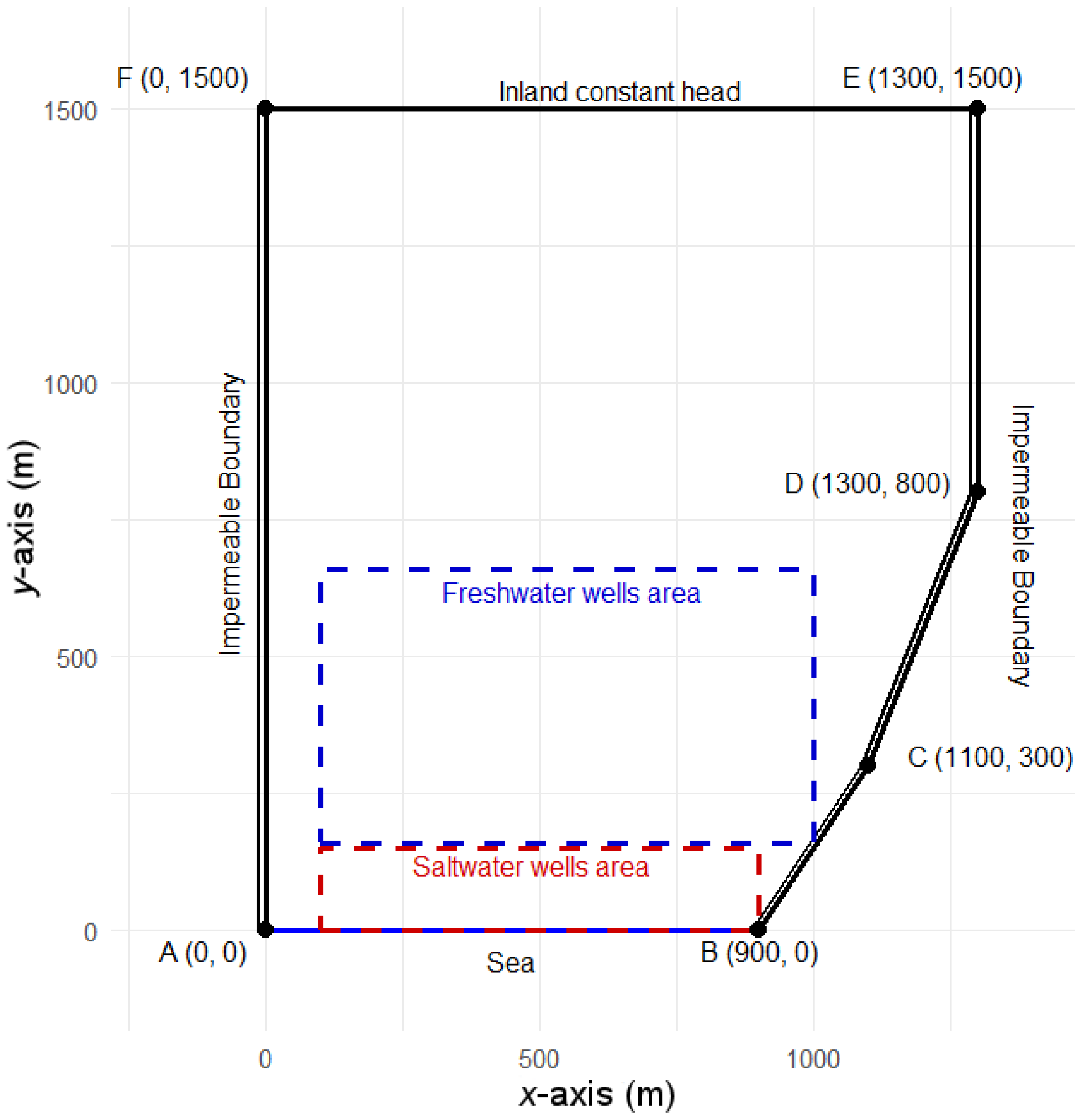
The optimization procedure of concurrent fresh and saltwater pumping optimization procedure is illustrated through the following application to the synthetic aquifer ABCDEF, which is shown in Figure 2. AB is the coastline, where the hydraulic head φ = 0. BCDE and FA are impermeable boundaries, while EF is a constant head boundary, with φ = 18 m. Influx of freshwater occurs through EF.

The problem is the following: There is a demand for freshwater (Q_DF = 150 L/s) and saltwater (Q_DS = 100 L/s) from the coastal aquifer ABCDEF. Two wells will be used for saltwater and three for freshwater pumping. The former should be constructed up to 150 m from the coast, while their x-coordinate should be between 100 and 900 m. The freshwater wells should be constructed further inland. Their y-coordinates should be between 160 and 660 m, and their x-coordinates between 100 and 1000 m. The areas available for the construction of saltwater and freshwater wells are shown in Figure 2 with red and blue broken lines, respectively. The hydraulic features of the coastal aquifer are: Transmissivity Tr = 0.005 m²/s, width b = 25 m, porosity θ = 0.1.

The optimization task is to find the locations and the flowrates of all five wells, that will not allow seawater intrusion to the freshwater wells. As mentioned in the previous sections, we have selected binary genetic algorithms as optimization tool. In the present study, each chromosome encodes the x and y coordinates and the flowrates of the five wells. We assume that flowrates can be between 0 and 100 L/s or between 0 and 150 L/s, for saltwater and freshwater wells, respectively. To represent a pair of coordinates (x_w and y_w) and one flowrate (Q_w) for each well in binary form the total chromosome length is 131. We assume that wells 1 and 2 are the saltwater wells and the remaining three are the freshwater ones.

Decoding the chromosomes to the decimal system can result in x, y values larger than their upper limits. To observe the respective constraints, we use corrective ratios. A similar procedure is used to ensure that the sum of saltwater and freshwater well flow rates is equal to 100 and 150 L/s, respectively. To this end, we calculate SQ_S, namely the sum of the flowrates of the “saltwater” wells, which result from chromosome decoding, and then we multiply each flowrate by the ratio 100/SQ_S. In the same way, the “freshwater” well flowrates are scaled to sum up to 150 L/s.

The optimization goal is to pump the required total freshwater and saltwater flowrates, without allowing seawater intrusion into freshwater wells. This should be depicted in the formulation of the optimization problem and the respective chromosome evaluation process. Extending previous approaches [31], we check whether the seawater inflow, Q_SEA, from the coast exceeds the required total saltwater flowrate, Q_DS. If it does, then the freshwater wells are certainly affected. On the contrary, it is not certain that, if Q_DS exceeds Q_SEA, freshwater wells are completely protected. It is quite probable, though, since they are constructed further from the coast, compared to the saltwater ones. Based on this thought, the optimization goal can be stated as:

$$\mathrm{m}\mathrm{i}\mathrm{n}\mathrm{i}\mathrm{m}\mathrm{i}\mathrm{z}\mathrm{e} Q_{SEA}- Q_{DS} \mathrm{i}\mathrm{f} Q_{SEA} > Q_{DS}$$

(1)

The problem constraints have the following forms:

$$Q_{SEA}\ge 0$$

(2)

$${\displaystyle \sum _{i=1}^2}{Q}_{wi}=Q_{DS}=100$$

(3)

$${\displaystyle \sum _{i=3}^5}{Q}_{wi}=Q_{DF}=150$$

(4)

$$100<x_i<900, i=1, 2$$

(5)

$$100<x_i<1000, i=3, 4, 5$$

(6)

$$0<y_i<150, i=1, 2$$

(7)

$$160<y_i<660, i=3, 4, 5$$

(8)

The chromosome fitness value FV₁ is expressed in the following way:

$${FV}_1=\left\{\begin{array}{c}{Q}_{SEA}-Q_{DS} \mathrm{i}\mathrm{f} Q_{SEA}>Q_{DS}\\ 0 \mathrm{i}\mathrm{f} Q_{SEA}\le Q_{DS}\end{array}\right.$$

(9)

Similar penalty-based criteria that link seawater intrusion risk to coastal influx or interface position have been employed in stochastic or metaheuristic optimization studies of coastal aquifers [32].

As shown in Equation (1), we have a minimization problem, with known best (minimum) value equal to zero. The calculation of Q_SEA requires simulation of the groundwater flow in the coastal aquifer. As the respective calculations are repeated for each chromosome of every generation, low computational volume is an important asset. The computational load of flow simulation models can be high, depending on the hydrogeological conditions, e.g., [33,34]. For this reason, a variety of surrogate models are often used [35,36,37,38]. We have opted for a boundary element code, which allows for straightforward calculations of inflows along the coastal boundary. Therefore, it combines low computational volume with high transferability to other coastal aquifers.

The basic features of the flow simulation model are the following. The field boundary is discretized in 51 boundary elements (9 on the coast AB, 14 on BCD, 13 on DE and 15 on DE). Data include coordinates of the boundary element endpoints, boundary type (constant head or impermeable) and field zone. The coefficients representing interactions between boundary elements are calculated only once. Well data are obtained from the genetic algorithm code. The respective coefficients must be calculated for every chromosome of each generation.

The values of the main parameters used in the genetic algorithm code have been selected based on experience from previous applications to similar problems, e.g., [39,40], where sensitivity analysis has been performed. They are: Population size, PS = 40; number of generations GN = 50; crossover probability CP = 0.55; mutation/antimetathesis probability MP = 0.011 $~$ 1.5/PS; tournament selection constant KK = 3.

The optimization-simulation code ends up with several different optimal solutions, namely with FV₁ = 0. A typical one is given in the second column of

Table 1. Typical best solutions for the two forms of the evaluation function (coordinates in m, flowrates in L/s).

Parameter	First Form of Evaluation Function (FV1)	Second Form of Evaluation Function (FV2)
FV	0	0
QSEA	95.379	100
xw(1)	551.22	755.33
yw(1)	137.65	132.35
Qw(1)	52.3	38.1
xw(2)	830.40	534.02
yw(2)	108.24	134.71
Qw(2)	47.7	61.9
xw(3)	263.64	629.62
yw(3)	490.72	644.34
Qw(3)	12.2	53.4
xw(4)	838.12	868.40
yw(4)	641.41	576.83
Qw(4)	65.4	71.8
xw(5)	954.25	413.20
yw(5)	646.30	599.33
Qw(5)	72.4	24.8

, together with the respective Q_SEA value. Q_SEA values generally vary from 95 to over 99.5 L/s. Convergence to an optimal solution across all runs is an additional indication that the choice of GA parameters was successful.

In practical applications the choice between solutions with similar FV values can be based on (a) additional criteria, not included in the chromosome evaluation process, (b) sensitivity of the solutions to input data, (c) frequency of appearance of each solution or (d) the experience of the user. We have opted to add one more criterion, which is related to the development of freshwater resources, namely maximization of seawater pumping by saltwater wells. The aim is to avoid any waste of freshwater. The importance of the second criterion is considered substantially smaller. This is depicted in the form of the chromosome’s fitness value FV₂ (Equation (10)). The penalty for excessive seawater influx includes a constant term, set equal to 5% of the influx limit. Moreover, the violation of the inflow limit is multiplied by 5.

$${FV}_2=\left\{\begin{array}{c}5+5\left(Q_{SEA}-Q_{DS}\right) \mathrm{i}\mathrm{f} Q_{SEA}>Q_{DS}\\ Q_{DS}-Q_{SEA} \mathrm{i}\mathrm{f} Q_{SEA}\le Q_{DS}\end{array}\right.$$

(10)

Again, we have a minimization problem, with known best (minimum) value equal to 0. This time, the code ends up with very few variations in the optimal solution, which corresponds to Q_SEA = Q_DS = 100 L/s. A typical optimal solution is shown in the third column of Table 1.

The chromosome evaluation process included a groundwater simulation model of low computational load. This is an important asset, since it should be run 40 × 50 = 2000 times. It may be accompanied, though, by some accuracy loss, regarding seawater intrusion into the freshwater wells. For this reason, the validity of the optimal solutions should be checked, using a more detailed simulation model. In the following paragraphs we have used two such models with different features, to compare their results and discuss the confidence degree.

3.2. Detailed Simulation Based on BEM and Particle Tracking

The first detailed numerical model combines the boundary element code to calculate groundwater velocities with a particle tracking (or moving point) code, to simulate seawater movement from the coast towards the wells. Four particles are initially placed along each boundary element of the coastline AB. So, we have 36 particles in total. Velocities V_x and V_y at each particle location are calculated directly using the values of φ and q on the boundary elements and they are considered as constant during each time-step ΔT, namely new particle locations are given by the following equations:

$$x_{in}=x_{io}+V_x·∆T$$

(11)

$$y_{in}=y_{io}+V_y·∆T$$

(12)

In Equations (11) and (12), x_io, y_io and x_in, y_in are the coordinates of the old and new particle locations, respectively. So, accuracy of x_in, y_in depends on ΔT magnitude. More technical details, regarding the arrival of particles to the wells, etc., can be found in the literature [40].

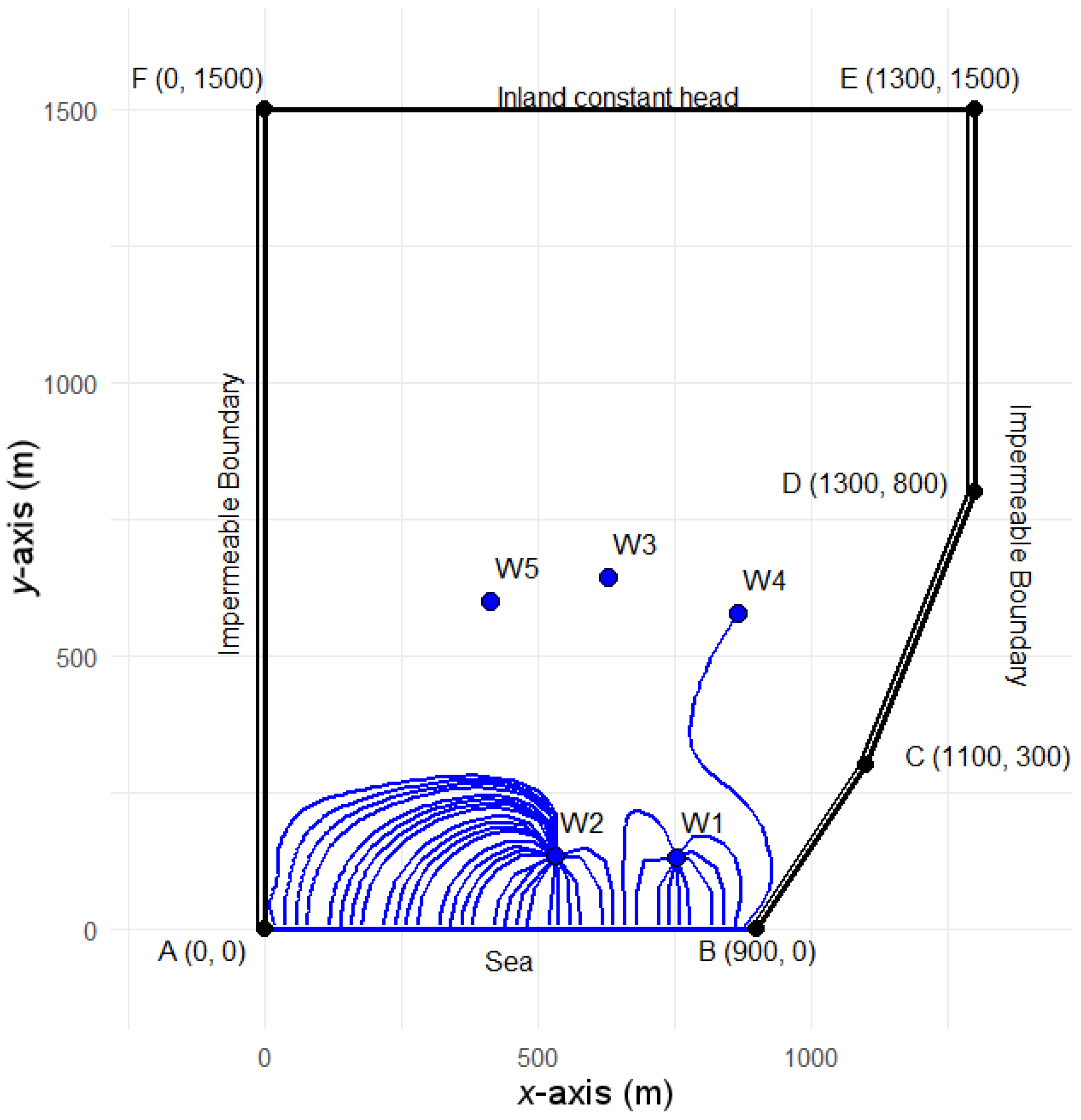
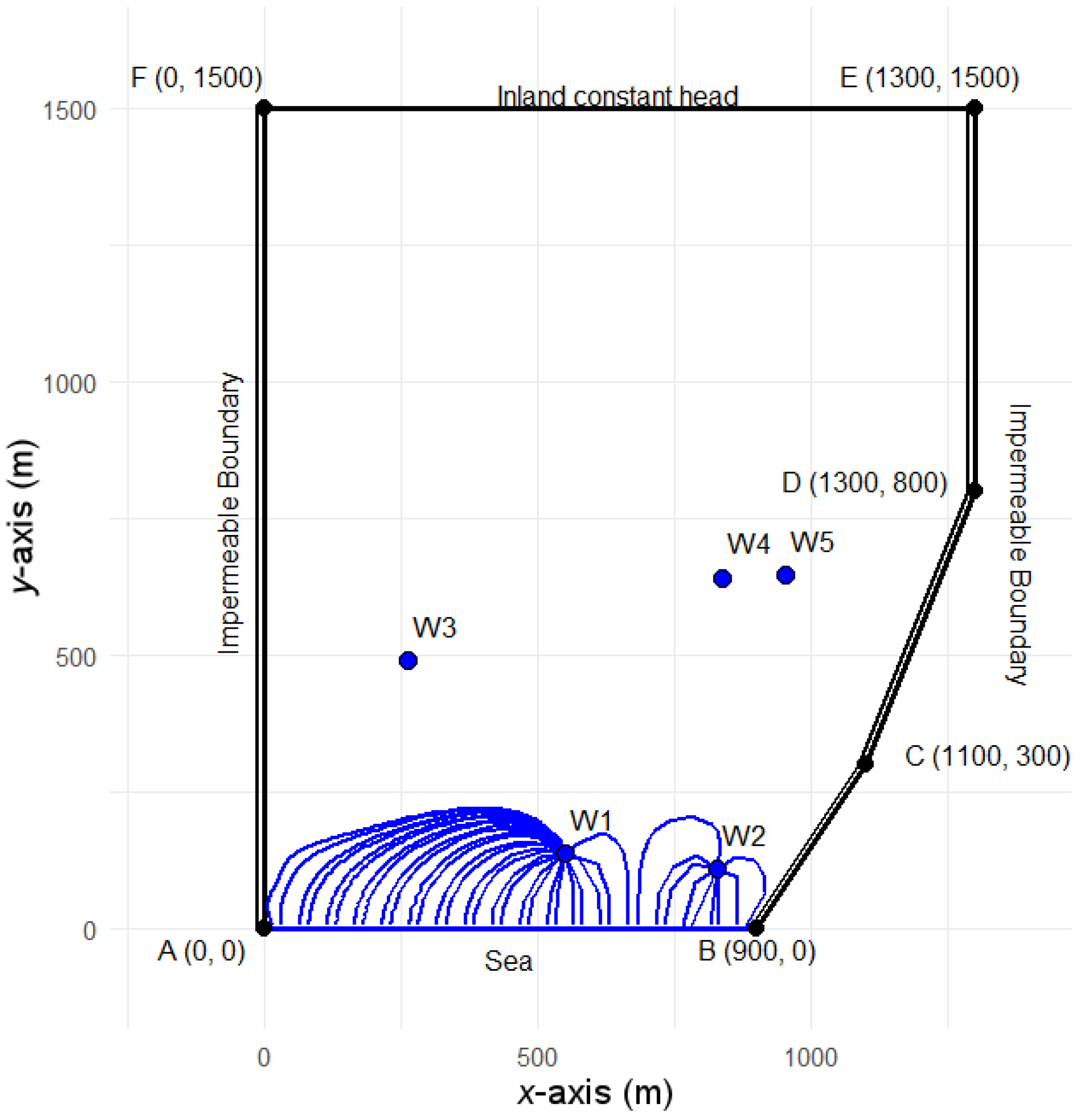
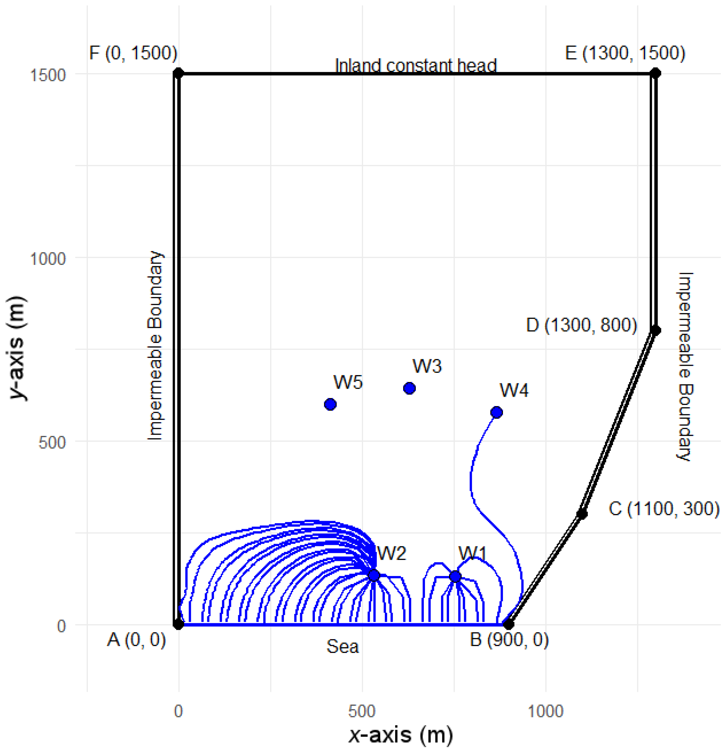
After some trials, we have concluded that a time-step ΔT = 0.2 d = 172,680 s is quite acceptable, since groundwater velocities are very low. The respective particle flow paths are shown in Figure 3 and Figure 4, for the two optimal solutions presented in Table 1. It can be seen that the well data of column 2 (corresponding to optimal solution using the first evaluation function) lead to complete protection of the freshwater wells. On the other hand, the set of well locations and flowrates of column 3 allows some saltwater intrusion into one freshwater well. It is rather small, though. The sea influx, corresponding to the particle which reached well 4, is equal to 4.5 L/s, namely it does not exceed 6.3% of the well flowrate, which is equal to 71.8 L/s.

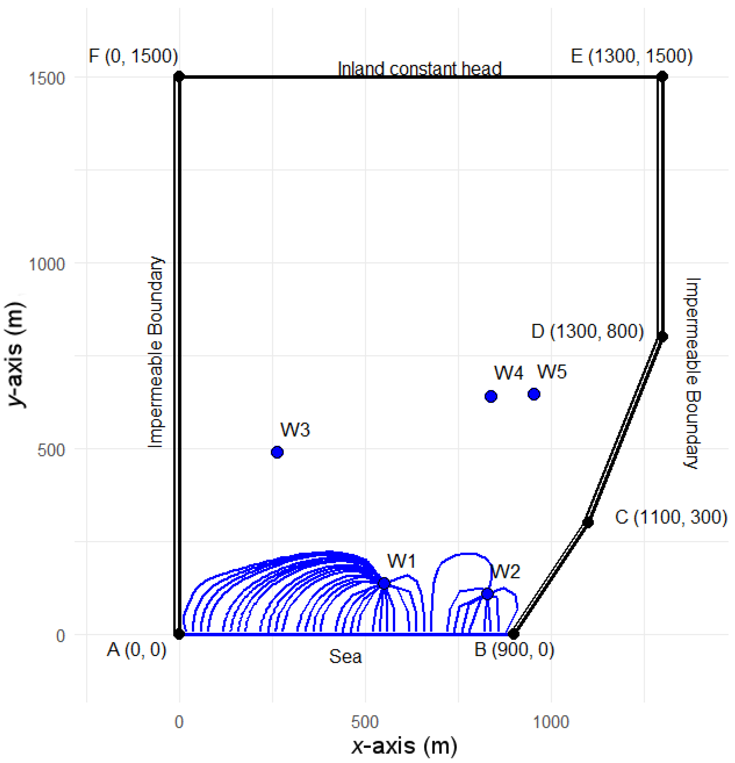
Moreover, to investigate the possible impact of discretization, we refined it along the coastal boundary, where we used 18 elements instead of 9, reducing their length from 100 m to 50 m. To facilitate comparisons, we did not change the total number of moving points. The groundwater flow patterns, shown in Figure 5 and Figure 6, are practically the same as those of Figure 3 and Figure 4, respectively. The well data of column 2 lead to complete protection of the freshwater wells, while those of column 3 allow some saltwater intrusion of one freshwater well. The sea influx to freshwater well 4 is 5.3 L/s, which is slightly larger than that obtained with the coarser boundary discretization. We conclude, then, that the discretization used in the optimization process was adequate.

Inflows through the coastal boundary elements for both optimal solutions and boundary discretizations are given in Tables S1 and S2 of the Supplementary Materials.

3.3. Detailed Simulation Using MODFLOW

The MODFLOW 6 GWF-GWT model was applied to both optimal solutions presented in Table 1. The model covers the same domain ABCDEF with the same boundary conditions and hydraulic parameters as the BEM model. The numerical domain is constructed using the Discretization by Vertices (DISV) approach, providing an unstructured grid with quadtree-based refinement via the Gridgen algorithm, yielding 18,370 active nodes per layer (91,850 in total). Cell size is 10 m × 10 m across the domain, but it is reduced to 1.25 m × 1.25 m near the wells. The aquifer is discretized into five horizontal layers of equal thickness (5 m), giving a total depth of 25 m. The simulation covers a single stress period of 720 days, divided into 240 time-steps of three days each.

Variable-density flow is handled via the Buoyancy (BUY) package, which implements a linear equation of state relating salt concentration to fluid density, with values ranging from 997 kg/m³ (for freshwater) to 1025 kg/m³ (for seawater at a reference salinity of 35 g/L). The transport engine uses an upstream weighting scheme for advection and incorporates mechanical dispersion and molecular diffusion to simulate spreading of freshwater–saltwater transition zone (the mixing interface between fresh and saline water) [41]. The dispersion parameters were selected to align with characteristic ratios cited in the seawater intrusion literature [42,43] and established hydrogeological standards. To satisfy the Péclet number criterion, horizontal longitudinal dispersivity ($a_L$) was set equal to the primary cell dimension ($a_L$ = 10 m). Following the standard hierarchy of dispersive spreading, transverse dispersivity ($a_T$) was defined as 10% of $a_L$ (1.0 m), while vertical longitudinal dispersivity ($a_v$) was constrained to 1% of $a_L$ (0.1 m). This anisotropic dispersivity tensor, combined with a molecular diffusion coefficient ($D_m$) of 8.64 $\times$ 10⁻⁵ m²/d, ensures a mathematically robust representation of the brackish transition zone.

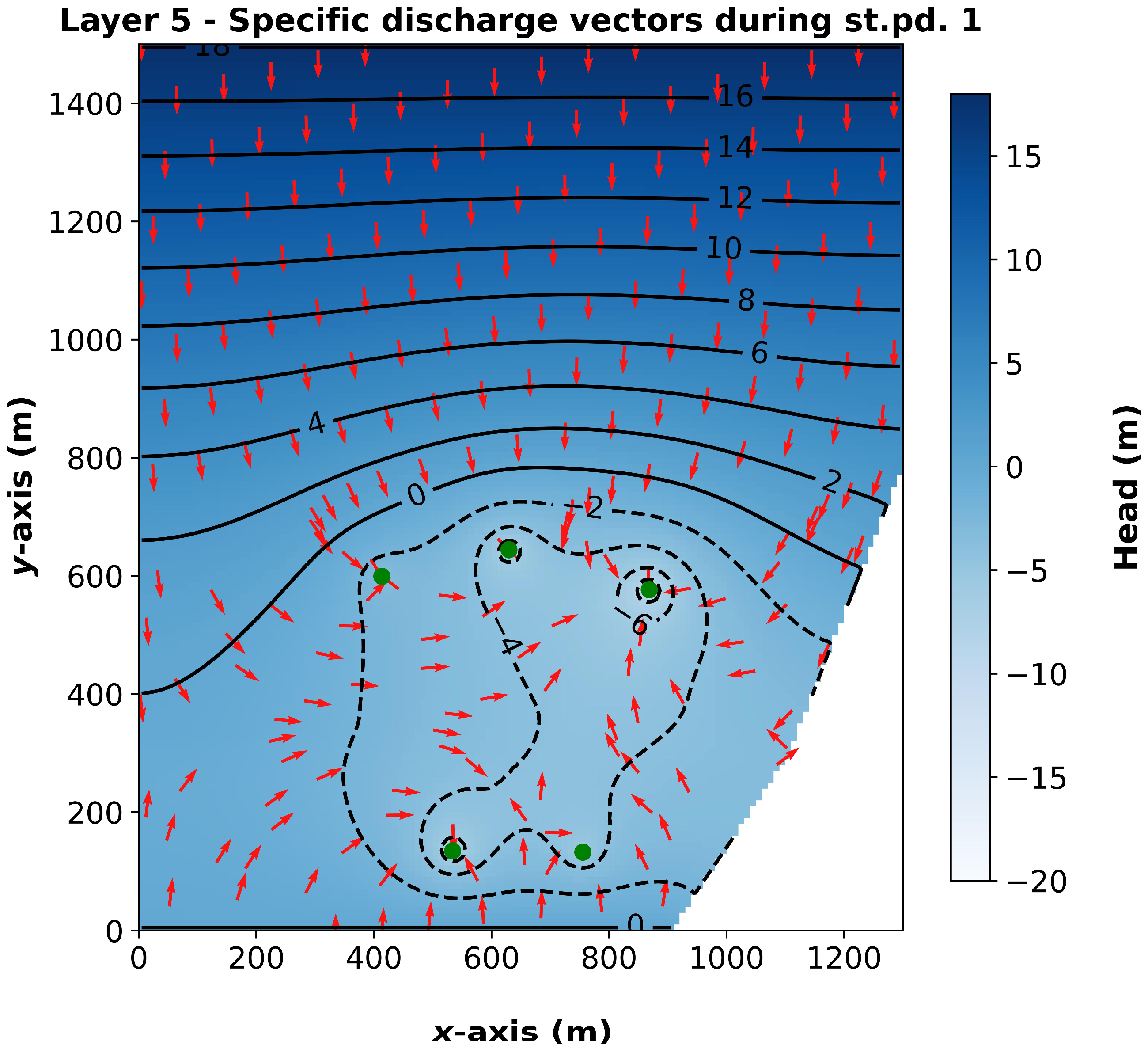
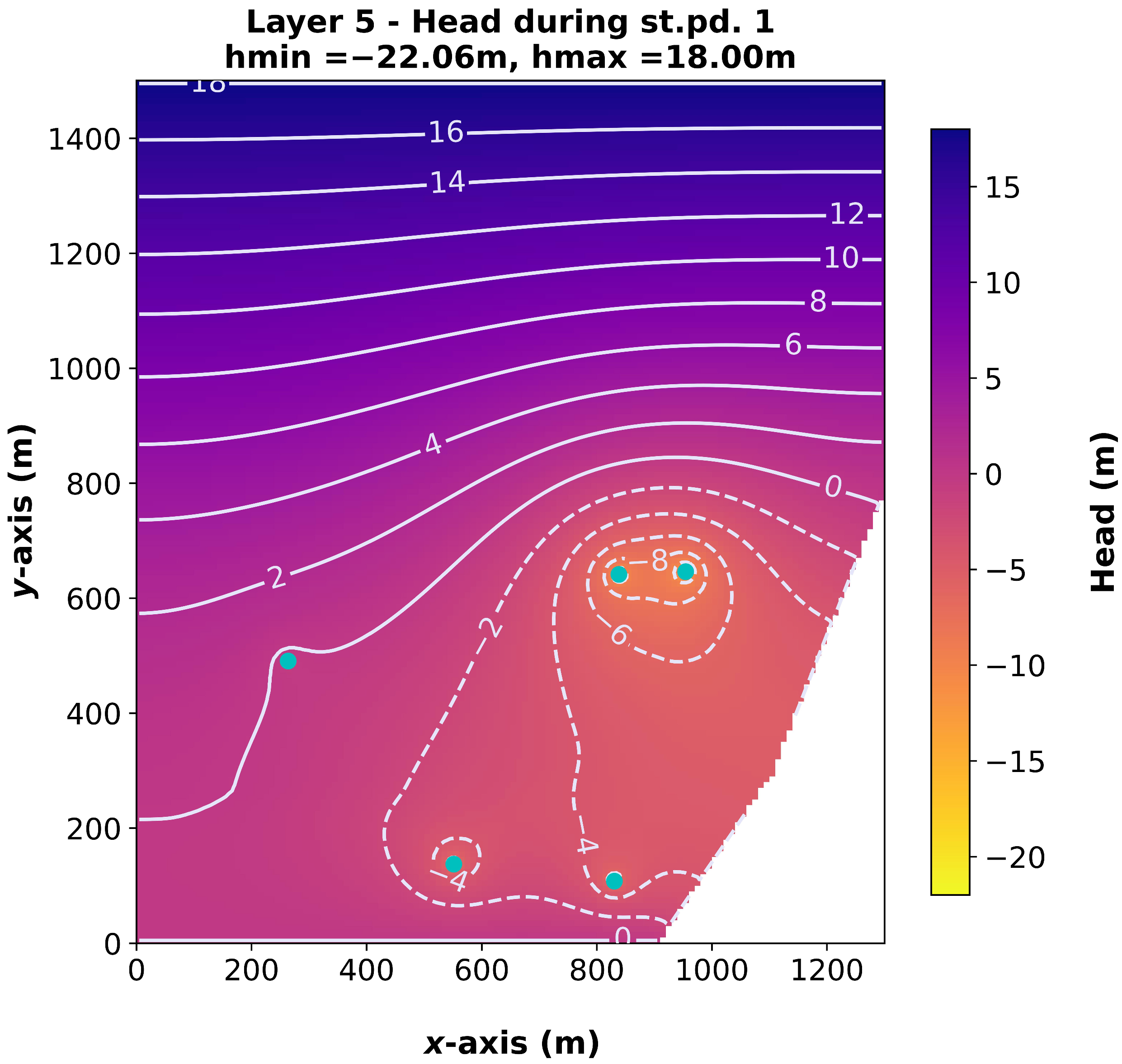
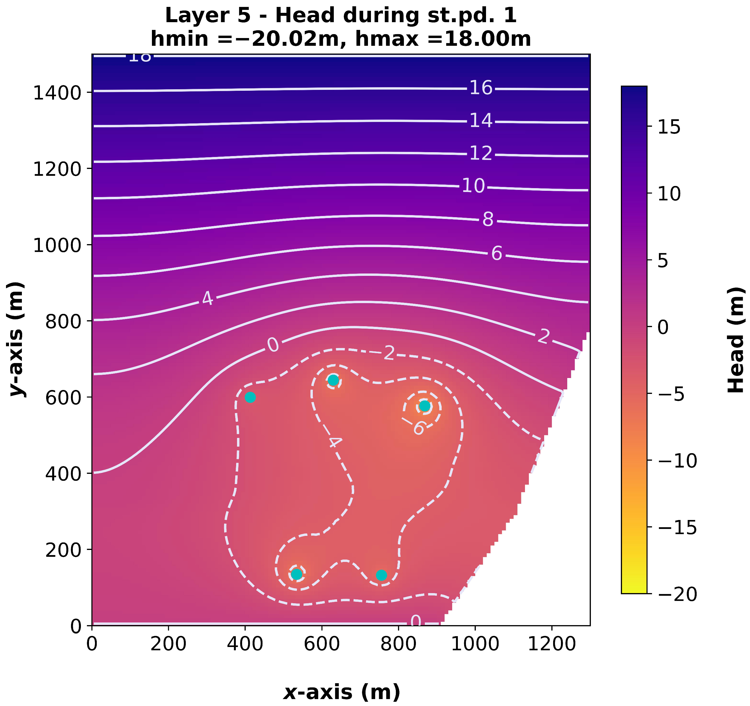
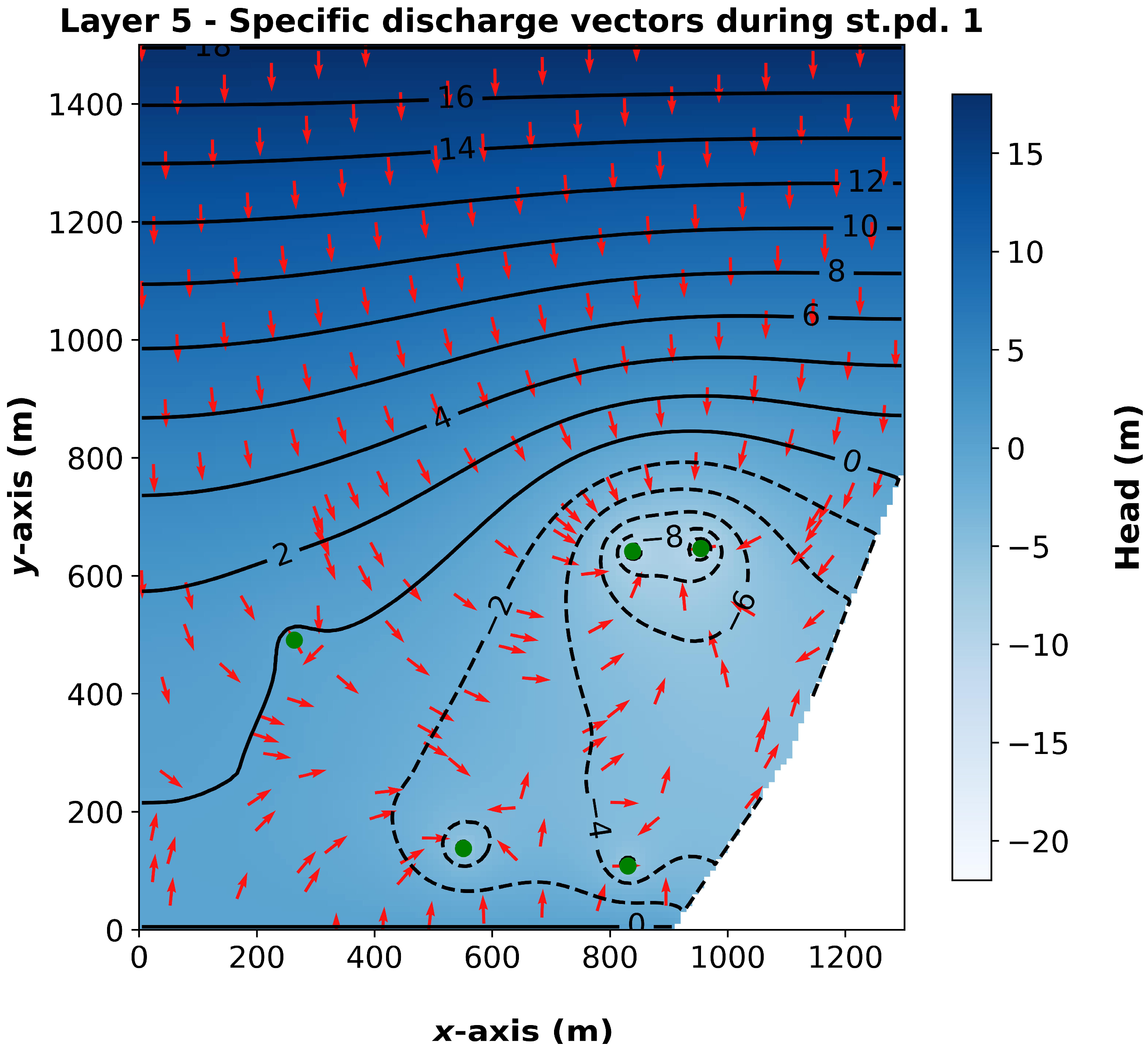
Results are presented for Layer 5 (bottom layer), which exhibits the most advanced saline wedge penetration; given that head distributions and specific discharge vectors are essentially layer-invariant, the corresponding maps are presented for Layer 5 only; salinity concentration maps for all remaining layers are provided in the Supplementary Materials. The head distributions for the optimal well layout resulting from evaluation functions FV₁ and FV₂ (Figure 7 and Figure 8) both show the expected gradient from the inland constant head boundary (φ = 18 m) towards the coast. Head depression around the pumping wells is also shown. The differences between the two scenarios are consistent with the differences between the well flowrates (and locations). The specific discharge vector maps (Figure 9 and Figure 10) confirm southward regional flow in the upper domain and convergence towards the pumping centers in the lower part. The total boundary fluxes, presented in

Table 2. Total volumetric boundary fluxes (L/s), for both optimal solutions using MODFLOW.

Boundary	FV1	FV2
Sea (inflow)	96.81	101.47
Inland boundary (inflow)	153.19	148.53

, show total seawater inflow of 96.8 L/s for FV₁ and 101.5 L/s for FV₂, both in close agreement with the target Q_DS = 100 L/s. Freshwater inflow through the inland boundary is 153.2 L/s and 148.5 L/s, respectively. In both cases, the total influx sums to Q_DF + Q_DS = 250 L/s.

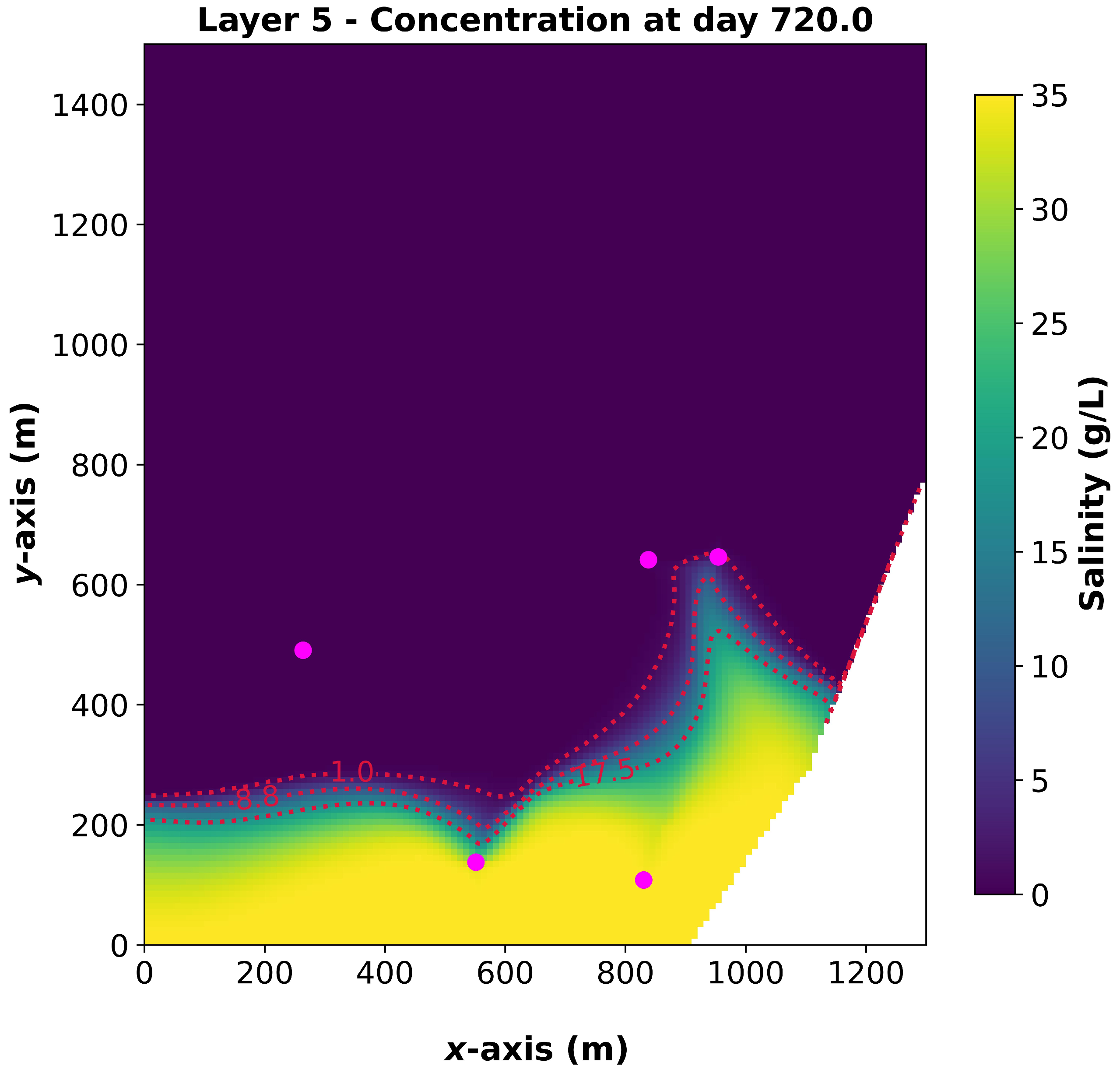
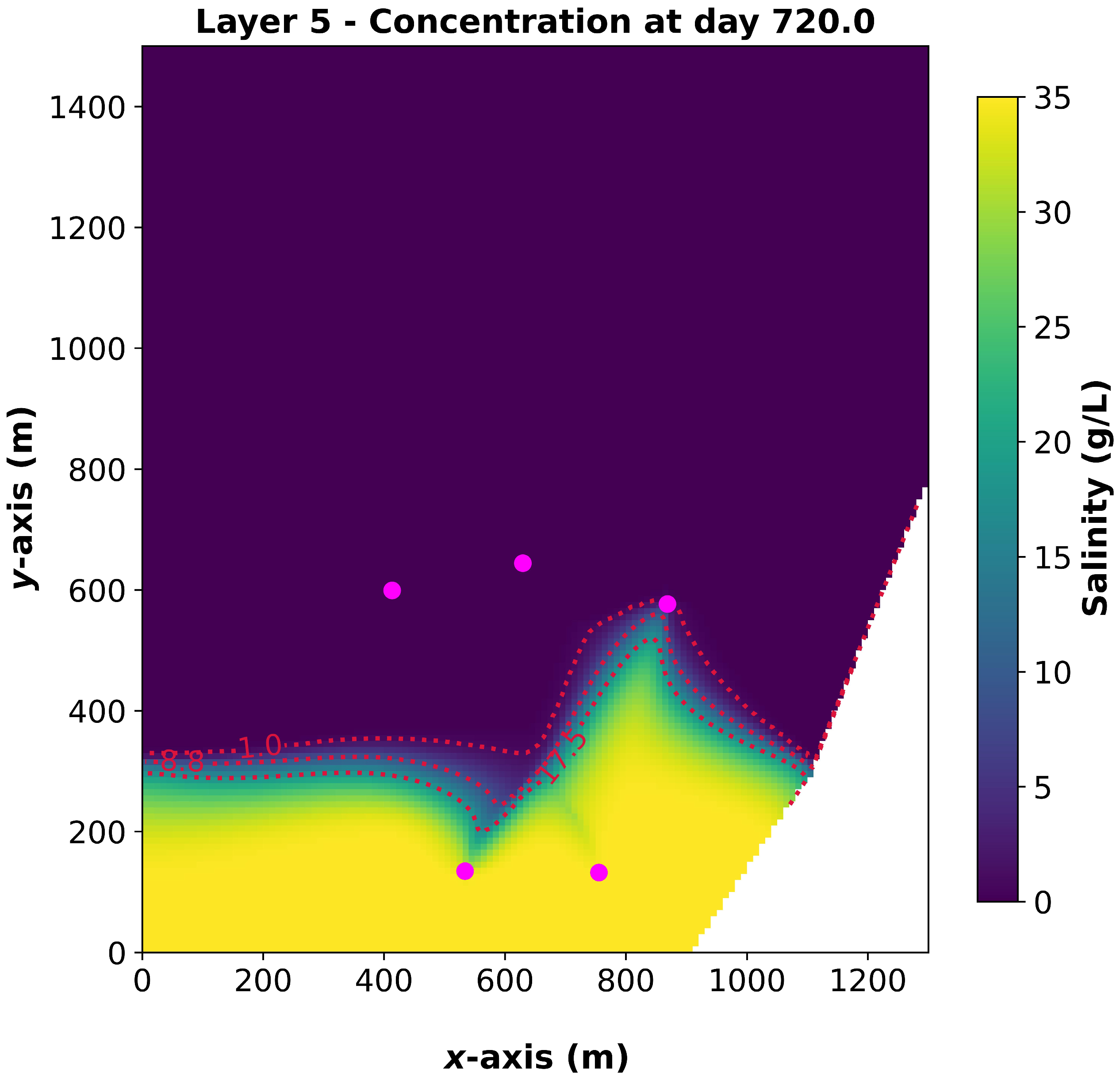
The salinity distributions at day 720 for both solutions are shown in Figure 11 and Figure 12. Under FV₁, the saltwater wedge occupies the coastal strip south of approximately y = 150 m in Layer 5 and is intercepted by the saltwater well pair. A saline “tongue” extends inland between x = 800–1000 m, with the 1 g/L isoline reaching y ≈ 650 m, approaching the freshwater wells W(4) and W(5). Under FV₂, the saltwater wedge occupies the coastal strip south of approximately y = 200 m in Layer 5 and is more spatially extensive than under FV₁. The 1 g/L isoline reaches y ≈ 300–320 m across the western part of the domain, and a saline “tongue” extends inland between x = 800–900 m, with the 1 g/L isoline reaching y ≈ 580 m, in the immediate vicinity of freshwater well W (4).

The temporal progression of salinity at the three freshwater wells for both solutions is shown in Figure 13 and summarized in

Table 3. Salinity (g/L) at freshwater wells W(3), W(4) and W(5), Layer 5, at selected time-steps for both optimal solutions using MODFLOW (columns 2, 3, 4 for FV₁ and 4, 6, 7 for FV₂).

Time (Days)	W(3)	W(4)	W(5)	W(3)	W(4)	W(5)
222	0.0	0.0	0.0	0.0	0.1	0.0
297	0.0	0.0	0.1	0.0	0.3	0.0
594	0.0	0.1	1.2	0.0	1.9	0.0
720	0.0	0.1	1.6	0.0	2.2	0.0

. Under FV₁, well W(3) (Q = 12.2 L/s) remains at 0.0 g/L throughout the simulation; well W(4) (Q = 65.4 L/s) shows only a marginal salinization, with Layer 5 reaching 0.1 g/L after day 594 and stabilizing; well W(5) (Q = 72.4 L/s) shows a continuous rising trend, with Layer 5 reaching 1.6 g/L by day 720. Under FV₂, well W(3) (Q = 53.4 L/s) remains completely unaffected (0.0 g/L); well W(5) (Q = 24.8 L/s) also remains at 0.0 g/L throughout the simulation; well W(4) (Q = 71.8 L/s), however, shows pronounced and continuous salinization from day 222 onwards, reaching 2.2 g/L at Layer 5 by day 720.

4. Discussion and Conclusions

Fair allocation of water to achieve socially fair and financially efficient development may be very challenging in coastal aquifers. Using saline groundwater to cover demand for non-potable water can contribute directly to conservation of freshwater resources, reducing the respective demand. If these two well systems are optimized together, an additional indirect benefit might be achieved, since saline water pumping, if properly planned, restricts progress of seawater intrusion towards inland freshwater wells.

In our paper, we have introduced a two-step methodology for concurrent optimization of fresh and saltwater pumping systems. In the first step, we combine genetic algorithms with a simulation tool, based on the Boundary Element Method. To keep the computational volume low, we introduce simple optimization criteria. This approach may lead to less accurate results, though. For this reason, additional evaluation of the selected optimal solutions, using more detailed flow simulation models, is a necessary final step.

We have used two quite different computational tools in this step. Comparing their results, we see that they are close to each other, but not identical. Both models lead to the conclusion that freshwater wells are better protected for the well layout resulting from FV₁. Nevertheless, MODFLOW predicted that two wells would be mildly affected after a long period of time, whereas the BEM-particle tracking scheme indicated that all freshwater wells would be safe. Regarding optimal solution resulting from FV₂, both codes indicated that well W(4) is vulnerable to pollution, although the salinization degree is expressed in different terms.

The aforementioned discrepancies should serve as a reminder that accuracy of results of computational models has limitations, due to assumptions made at the conceptual, mathematical and numerical level, besides those due to insufficient data. In optimization problems, the statement of the optimization goals is an additional concern.

In any case the two tools, used in this paper, are indicative. The choice for any specific case study may vary, depending on tool availability and even on the experience and the subjective preferences of the scientists involved.

The overall computational load of the proposed two-step methodology can be considered as an important asset. Compared to the use of surrogate models in the simulation-optimization procedure, e.g., [44], it does not require a training phase, while its second step, namely the detailed simulation of the aquifer, is executed one time only. Moreover, the second step may provide an estimate of the accuracy of the optimization process.

The addition of optimization criteria does not guarantee overall improvement of the optimization results, as they will essentially represent a tradeoff between the criteria used. In our example, the variety of the optimal solutions, obtained using the first criterion only (keeping sea influx lower than the total seawater demand), prompted us to include an additional criterion, namely avoidance of freshwater pumping from saltwater wells. We found out that fulfillment of the second criterion compromised the main target of the optimization task, namely full protection of freshwater wells, although we explicitly attributed smaller importance to it. The reason is that it resulted in elimination of the difference between saltwater demand Q_DS and seawater influx Q_SEA, which serves as an implicit safety factor for the protection of the freshwater wells.

It follows that solutions that better protect the freshwater wells can be found by lowering the limit of Q_SEA to a percentage of Q_DS. The chromosome evaluation function, given by Equation (9), can be easily adjusted.

The use of saline abstraction near the coast as a hydraulic barrier against seawater intrusion is a well-established management strategy [45], with analytical grounding provided by Vandenberg [46], who showed that a saltwater well sited between the coast and a freshwater well can substantially increase the allowable freshwater yield. Field modeling studies confirm the practical relevance of saline abstraction as a management tool, as demonstrated in Wadi Ham (UAE) [47]. As with these field cases, optimal well configurations are inherently site-specific [47], and the results of the present study should be interpreted accordingly. The proposed methodology should therefore be regarded as a flexible framework for systematically exploring the feasible design space and formulating hypotheses about effective well roles (freshwater extraction and saline interception), which can subsequently be adapted to any specific application using site-calibrated models.

Finally, it can be concluded that the methodology described in this paper can contribute to the concurrent optimization of freshwater and saltwater pumping systems in coastal aquifers.

References

1. Valipour, E.E.; Ketabchi, H.; Safari shali, R.; Morid, S. Equity, Social Welfare, and Economic Benefit Efficiency in the Optimal Allocation of Coastal Groundwater Resources. Water Resour. Manag. 2023, 37, 2969–2990. [Google Scholar] [CrossRef] [Scilit]
2. Tang, S.L.; Yue, D.P.T.; Ku, D.C.C. Engineering and Costs of Dual Water Supply Systems; IWA Publishing: London, UK; Seattle, WA, USA, 2007; ISBN 978-184-339-132-6. [Google Scholar]
3. Beltrán, J. Irrigation with saline water: Benefits and environmental impact. Agric. Water Manag. 1999, 40, 183–194. [Google Scholar] [CrossRef] [Scilit]
4. Li, P.; Ren, L. Evaluating the saline water irrigation schemes using a distributed agro-hydrological model. J. Hydrol. 2020, 594, 125688. [Google Scholar] [CrossRef] [Scilit]
5. Zhou, S.; Wang, G.; Zhang, J.; Dang, H.; Gao, Y.; Sun, J. Long-term saline water irrigation has the potential to balance greenhouse gas emissions and cotton yield in North China plain. J. Environ. Manag. 2024, 352, 120087. [Google Scholar] [CrossRef] [Scilit]
6. Al-Muaini, A.; Green, S.; Dakheel, A.; Abdullah, A.; Sallam, O.; Dahr, W.; Dixon, S.; Kemp, P.; Clothier, B. Water requirements for irrigation with saline groundwater of three date-palm cultivars with different salt-tolerances in the hyper-arid United Arab Emirates. Agric. Water Manag. 2019, 222, 213–220. [Google Scholar] [CrossRef] [Scilit]
7. Ge, Y.; Jia, Y.; Li, S.; Jie, F. Optimization of Freshwater–Saline Water Resource Mixing Irrigation Under Multiple Constraints. Sustainability 2025, 17, 3729. [Google Scholar] [CrossRef] [Scilit]
8. Zhou, Q.; Lyu, D.; Li, W.; Wen, Y.; Wang, Z. Effects of Irrigation Amount and Salinity Levels on Maize (Zea mays L.) Growth, Water Productivity and Carbon Emissions in Arid Region of Northwest China. Agronomy 2024, 14, 2656. [Google Scholar] [CrossRef] [Scilit]
9. Cao, Y.; Zhang, Y.; Zhao, Y.; Wang, C.; Niu, Z. Interactions and Integrated Optimization between Secondary Water Supply Devices and Drinking Water Distribution Systems: A Review. Water Resour. Manag. 2025, 39, 3625–3639. [Google Scholar] [CrossRef] [Scilit]
10. Park, C.; Aral, M. Multi-objective optimization of pumping rates and well placement in coastal aquifers. J. Hydrol. 2004, 290, 80–99. [Google Scholar] [CrossRef] [Scilit]
11. Cheng, A.; Halhal, D.; Naji, A.; Ouazar, D. Pumping optimization in saltwater-intruded coastal aquifers. Water Resour. Res. 2000, 36, 2155–2165. [Google Scholar] [CrossRef] [Scilit]
12. Holland, J.H. Adaptation in Natural and Artificial Systems; University of Michigan Press: Ann Arbor, MI, USA, 1975. [Google Scholar]
13. Katsifarakis, K.L.; Karpouzos, K.D.; Theodossiou, N. Combined use of BEM and genetic algorithms in groundwater flow and mass transport problems. Eng. Anal. Bound. Elem. 1999, 23, 555–565. [Google Scholar] [CrossRef] [Scilit]
14. Brebbia, C.A. The Boundary Element Method for Engineers; Pentech Press: London, UK, 1978. [Google Scholar]
15. Katsikadelis, J.T. The Boundary Element Method for Engineers and Scientists. Theory and Applications, 2nd ed.; Elsevier: London, UK, 2016. [Google Scholar]
16. Gwinner, J.; Stephan, E.P. Advanced Boundary Element Methods. Treatment of Boundary Value, Transmission and Contact Problems; Springer: Berlin/Heidelberg, Germany, 2018. [Google Scholar]
17. Kirkup, S. The Boundary Element Method in Acoustics: A Survey. Appl. Sci. 2019, 9, 1642. [Google Scholar] [CrossRef] [Scilit]
18. Kleanthous, A.; Baran, A.J.; Betcke, T.; Hewett, D.P.; Westbrook, C.D. An application of the boundary element method (BEM) to the calculation of the single-scattering properties of very complex ice crystals in the microwave and sub-millimetre regions of the electromagnetic spectrum. J. Quant. Spectrosc. Radiat. Transf. 2024, 312, 108793. [Google Scholar] [CrossRef] [Scilit]
19. Xu, Y.; Jackson, R.L. Boundary element method (BEM) applied to the rough surface contact vs. BEM in computational mechanics. Friction 2019, 7, 359–371. [Google Scholar] [CrossRef] [Scilit]
20. El Harrouni, K.; Ouazar, D.; Walters, G.A.; Cheng, A.H.-D. Groundwater optimization and parameter estimation by genetic algorithm and dual reciprocity boundary element method. Eng. Anal. Bound. Elem. 1996, 18, 287–296. [Google Scholar] [CrossRef] [Scilit]
21. Lesnic, D.; Elliott, L.; Ingham, D.B. A boundary element method for the determination of the transmissivity of a heterogeneous aquifer in groundwater flow systems. Eng. Anal. Bound. Elem. 1998, 21, 223–234. [Google Scholar] [CrossRef] [Scilit]
22. Luo, W.; Wang, J.; Wang, L.; Zhou, Y. An alternative BEM for simulating the flow behavior of a leaky confined fractured aquifer with the use of the semianalytical approach. Water Resour. Res. 2020, 56, e2019WR026581. [Google Scholar] [CrossRef] [Scilit]
23. Katsifarakis, K.L.; Kontos, Y.N.; Keremidis, O. Evaluation of analytical solutions based on the assumption of one-dimensional groundwater flow using numerical solutions for two-dimensional flows. Hydrology 2025, 12, 226. [Google Scholar] [CrossRef] [Scilit]
24. Zabala, I.; Henriques, J.C.C.; Kelly, T.E.; Ricci, P.P.; Blanco, J.M. Post-processing techniques to improve the results of hydrodynamic Boundary Element Method solvers. Ocean Eng. 2024, 295, 116913. [Google Scholar] [CrossRef] [Scilit]
25. Liu, Y.J.; Mukherjee, S.; Nishimura, N.; Schanz, M.; Ye, W.; Sutradhar, A.; Pan, E.; Dumont, N.A.; Frangi, A.; Saez, A. Recent Advances and Emerging Applications of the Boundary Element Method. ASME. Appl. Mech. Rev. 2011, 64, 030802. [Google Scholar] [CrossRef] [Scilit]
26. Katsifarakis, K.L.; Petala, Z. Combining genetic algorithms and boundary elements to optimize coastal aquifers’ management. J. Hydrol. 2006, 327, 200–207. [Google Scholar] [CrossRef] [Scilit]
27. Klaas, D.K.S.Y.; Imteaz, M.A.; Arulrajah, A. Development of groundwater vulnerability zones in a data-scarce eogenetic karst area using Head-Guided Zonation and particle-tracking simulation methods. Water Res. 2017, 122, 17–26. [Google Scholar] [CrossRef] [Scilit] [PubMed]
28. McDonald, M.G.; Harbaugh, A.W. A Modular Three-Dimensional Finite-Difference Ground-Water Flow Model (Techniques of Water-Resources Investigations, Book 6, Chapter A1); U.S. Geological Survey: Reston, VA, USA, 1988.
29. Harbaugh, A.W. MODFLOW-2005, the U.S. Geological Survey Modular Ground-Water Model: The Ground-Water Flow Process (Techniques and Methods 6-A16); U.S. Geological Survey: Reston, VA, USA, 2005.
30. Langevin, C.D.; Hughes, J.D.; Banta, E.R.; Niswonger, R.G.; Provost, A.M.; Panday, S.; Winston, R.B. Documentation for the MODFLOW 6 Groundwater Flow Model (Techniques and Methods 6-A55); U.S. Geological Survey: Reston, VA, USA, 2017.
31. Langevin, C.D.; Provost, A.M.; Panday, S.; Hughes, J.D. Documentation for the MODFLOW 6 Groundwater Transport Model (Techniques and Methods 6-A61); U.S. Geological Survey: Reston, VA, USA, 2022.
32. Stratis, P.; Karatzas, G.; Papadopoulou, E.; Zakynthinaki, M.; Saridakis, Y. Stochastic Optimization for an Analytical Model of Saltwater Intrusion in Coastal Aquifers. PLoS ONE 2016, 11, e0162783. [Google Scholar] [CrossRef] [Scilit] [PubMed]
33. Doulgeris, C.; Zissis, T. 3D Variable Density Flow Simulation to Evaluate Pumping Schemes in Coastal Aquifers. Water Resour. Manag. 2014, 28, 4943–4956. [Google Scholar] [CrossRef] [Scilit]
34. Masciopinto, C.; Liso, I.S.; Caputo, M.C.; De Carlo, L. An Integrated Approach Based on Numerical Modelling and Geophysical Survey to Map Groundwater Salinity in Fractured Coastal Aquifers. Water 2017, 9, 875. [Google Scholar] [CrossRef] [Scilit]
35. Christelis, V.; Regis, R.G.; Mantoglou, A. Surrogate-based pumping optimization of coastal aquifers under limited computational budgets. J. Hydroinform. 2018, 20, 164–176. [Google Scholar] [CrossRef] [Scilit]
36. Roy, D.K.; Datta, B. A review of surrogate models and their ensembles to develop saltwater intrusion management strategies in coastal aquifers. Earth Syst. Environ. 2018, 2, 193–211. [Google Scholar] [CrossRef] [Scilit]
37. Christelis, V.; Kopsiaftis, G.; Regis, R.G.; Mantoglou, A. An adaptive multi-fidelity optimization framework based on co-Kriging surrogate models and stochastic sampling with application to coastal aquifer management. Adv. Water Resour. 2023, 180, 104537. [Google Scholar] [CrossRef] [Scilit]
38. Sharan, A.; Roy, D.K.; Datta, B.; Lal, A. A multi-objective simulation-optimisation model for managing saltwater intrusion in a coastal aquifer of the Pacific Island of Vanuatu. J. Hydrol. 2026, 669, 135128. [Google Scholar] [CrossRef] [Scilit]
39. Kontos, Y.N.; Katsifarakis, K.L. Optimal management of a theoretical coastal aquifer with combined pollution and salinization problems, using genetic algorithms. Energy 2017, 136, 32–44. [Google Scholar] [CrossRef] [Scilit]
40. Kontos, Y.N.; Katsifarakis, K.L. Optimization of Management of Polluted Fractured Aquifers Using Genetic Algorithms. Eur. Water 2012, 40, 31–42. [Google Scholar]
41. Voss, C.I.; Souza, W.R. Variable density flow and solute transport simulation of regional aquifers containing a narrow freshwater-saltwater transition zone. Water Resour. Res. 1987, 23, 1851–1866. [Google Scholar] [CrossRef] [Scilit]
42. Agossou, A.; Yang, J.-S.; Lee, J.-B. Evaluation of Potential Seawater Intrusion in the Coastal Aquifers System of Benin and Effect of Countermeasures Considering Future Sea Level Rise. Water 2022, 14, 4001. [Google Scholar] [CrossRef] [Scilit]
43. Chang, Q.; Gao, C.; Zheng, X.; Lin, Y.; Song, X. A novel subsurface adjustable dam for preventing active seawater intrusion in coastal aquifers. Front. Mar. Sci. 2024, 11, 1412052. [Google Scholar] [CrossRef] [Scilit]
44. Christelis, V.; Kopsiaftis, G.; Mantoglou, A. Performance comparison of multiple and single surrogate models for pumping optimization of coastal aquifers. Hydrol. Sci. J. 2019, 64, 336–349. [Google Scholar] [CrossRef] [Scilit]
45. Hussain, M.S.; Abd-Elhamid, H.F.; Javadi, A.A.; Sherif, M.M. Management of Seawater Intrusion in Coastal Aquifers: A Review. Water 2019, 11, 2467. [Google Scholar] [CrossRef] [Scilit]
46. Vandenberg, A. Simultaneous Pumping of Fresh and Salt Water from a Coastal Aquifer. J. Hydrol. 1975, 24, 37–43. [Google Scholar] [CrossRef] [Scilit]
47. Sowe, M.A.; Sathish, S.; Greggio, N.; Mohamed, M.M. Optimized Pumping Strategy for Reducing the Spatial Extent of Saltwater Intrusion along the Coast of Wadi Ham, UAE. Water 2020, 12, 1503. [Google Scholar] [CrossRef] [Scilit]
Figure 1. Flowchart of the proposed two-step optimization–validation methodology.
Water 18 01221 g001
Figure 2. Plan view of the synthetic aquifer (including the well construction zones).
Water 18 01221 g002
Figure 3. Seawater intrusion for the typical optimal solution resulting from FV1.
Water 18 01221 g003
Figure 4. Seawater intrusion for the optimal solution resulting from FV2.
Water 18 01221 g004
Figure 5. Seawater intrusion for the typical optimal solution resulting from FV1 using the finer coast boundary discretization.
Water 18 01221 g005
Figure 6. Seawater intrusion for the typical optimal solution resulting from FV2 using the finer coast boundary discretization.
Water 18 01221 g006
Figure 7. Hydraulic head distribution (m), Layer 5, for the optimal well layout resulting from FV1 using MODFLOW. Wells are represented by cyan dots. Dashed head contours represent negative head values.
Water 18 01221 g007
Figure 8. Hydraulic head distribution (m), Layer 5, for the optimal well layout resulting from FV2 using MODFLOW. Wells are represented by cyan dots. Dashed head contours represent negative head values.
Water 18 01221 g008
Figure 9. Specific discharge vectors (red arrows) and head contours, Layer 5, for the optimal well layout resulting from FV1 using MODFLOW. Wells are represented by green dots. Dashed head contours represent negative head values.
Water 18 01221 g009
Figure 10. Specific discharge vectors (red arrows) and head contours, Layer 5, for the optimal well layout resulting from FV2 using MODFLOW. Wells are represented by green dots. Dashed head contours represent negative head values.
Water 18 01221 g010
Figure 11. Seawater intrusion at day 720, Layer 5, for the optimal well layout resulting from FV1 using MODFLOW. Wells are represented by magenta dots. Red dashed lines denote salinity contours corresponding to 50% (17.5 g/L) and 25% (8.8 g/L) of the reference seawater salinity (35 g/L), along with the 1.0 g/L contour.
Water 18 01221 g011
Figure 12. Seawater intrusion at day 720, Layer 5, for the optimal well layout resulting from FV2 using MODFLOW. Wells are represented by magenta dots. Red dashed lines denote salinity contours corresponding to 50% (17.5 g/L) and 25% (8.8 g/L) of the reference seawater salinity (35 g/L), along with the 1.0 g/L contour.
Water 18 01221 g012
Figure 13. Temporal progression of salinity (g/L) at freshwater wells W(3), W(4) and W(5), Layer 5, over the 720-day simulation for the optimal well layout resulting from FV1 and FV2 using MODFLOW. Wells W(3) (both solutions) and W(5)–FV2 register 0.0 g/L throughout the simulation and overlap on the x-axis.
Water 18 01221 g013