Urban Flood Prediction Model Based on Transformer-LSTM-Sparrow Search Algorithm

Abstract

Global climate change and accelerated urbanization have intensified extreme rainfall events, exacerbating urban flood risks. Although data-driven models have shown potential in urban flood prediction, the ability of single models to capture complex nonlinear relationships and their sensitivity to hyperparameters still limit prediction accuracy. To address these challenges, this study proposes an urban flood prediction model by integrating Transformer, Long Short-Term Memory (LSTM), and Sparrow Search Algorithm (SSA), combining Transformer’s global feature extraction with LSTM’s temporal modeling. The SSA was adopted to optimize hyperparameters for the Transformer-LSTM model. Dropout and early stopping techniques were adopted to mitigate overfitting. Applied to Zhengzhou city of Henan province, China, the model achieves a Nash-Sutcliffe Efficiency (NSE) of 0.971, indicating that the proposed model has high prediction performance for urban flooding. The experimental results demonstrate that the Transformer-LSTM-SSA model outperforms the standalone Transformer, LSTM, and Transformer-LSTM models by 12.9%, 10.1%, and 2.9% in NSE accuracy, respectively, while reducing MAE by 62.12%, 56.9%, and 34.21%, respectively, and MAPE by 21.69%, 22.2%, and 10.89%, respectively. Furthermore, the proposed model exhibits enhanced stability and superior generalization capability. The Transformer-LSTM-SSA model exhibits superior performance among the comparative methods, thereby demonstrating the model’s viability for providing a reliable solution for real-time flood prediction and early warning.

1. Introduction

Under the influence of climate change and urbanization, the frequency and intensity of urban flooding have exhibited an increasing trend [1]. In recent years, severe urban waterlogging has affected many major cities worldwide, significantly disrupting lives, economies, and ecosystems [2,3]. Urban flood disasters have raised widespread societal concern. The “7·20” extreme rainfall event in 2021 in Zhengzhou, Henan Province caused catastrophic urban flooding across the region, directly affecting approximately 13.91 million residents and resulting in 380 fatalities alongside direct economic losses totaling RMB 40.9 billion [4]. Accurate flood prediction is crucial for reducing casualties and socio-economic losses. It provides a scientific basis for the formulation of flood control measures and emergency response, thereby effectively reducing the risks of flood disasters [5]. It is essential to establish a rapid and accurate prediction model for urban flood management.

Over the past decades, various approaches and models have been developed to simulate rainfall–flood processes in urban flood forecasting, including numerical models and data-driven models [6]. Although numerical models effectively characterize physical processes and provide interpretability, they require extensive hydrological data and considerable computational resources [7]. These limitations hinder their widespread application in real-time urban flood forecasting [8,9]. Data-driven models offer distinct advantages in computational efficiency and practical application [10,11]. These models can handle large-scale, high-dimensional data and directly learn complex nonlinear relationships in hydrological processes from historical data. For instance, Li et al. [12] applied an ANN model for predicting seawater intrusion run-up distance, demonstrating the significant advantages of data-driven modeling approaches. Data-driven models, such as deep learning and machine learning, have emerged as a pivotal direction in urban flood prediction.

Long Short-Term Memory (LSTM), a classical and robust time series prediction model, has achieved significant progress in flood forecasting, emerging as a key technique for predicting river discharge, groundwater levels, and urban flooding [13,14,15]. However, existing methods still face several challenges. Urban flooding is influenced by multiple interacting factors characterized by both temporal dependencies and complex nonlinear correlations [16,17]. While LSTM models effectively capture temporal sequences, they struggle to comprehensively represent these intricate relationships, resulting in accuracy limitations for urban flood prediction [11,18]. Transformer models, with their efficient parallel computation and powerful information-capturing capabilities [19,20], can selectively focus on task-relevant features through multi-head self-attention mechanisms, thereby better capturing critical input information [21]. Although Transformers are computationally intensive for long sequences, this limitation is mitigated in urban flood prediction due to the short-duration nature of rainfall–flood processes [22]. In hydrology, integrating Transformer with LSTM represents a novel research direction. For instance, Li et al. [23] fused LSTM as a feature extraction module with an improved Transformer for flood forecasting, where input information is first enhanced by LSTM and then predicted by Transformer. However, this approach may constrain the Transformer’s global feature extraction ability due to LSTM’s limited feature representation capacity. Guo et al. [24] separately applied LSTM and Transformer to predict different input components of monthly runoff sequences and combined their results. A limitation of this method lies in the potentially insufficient integration of information due to the independent predictions of LSTM and Transformer.

Additionally, model integration increases the complexity of hyperparameters and architectures. To address hyperparameter optimization, many researchers have employed metaheuristic algorithms [25,26]. Metaheuristic algorithms outperform conventional methods by simulating natural systems to locate global optima, while providing simpler implementation, fewer tuning parameters, and better avoidance of local optima [27]. The Sparrow Search Algorithm (SSA) is a novel metaheuristic algorithm proposed by Xue and Shen [28]. Existing scholarly research has demonstrated that the SSA exhibits superior optimization performance compared to alternative metaheuristic approaches, including the Grey Wolf Optimizer (GWO), Particle Swarm Optimization (PSO), and Gravitational Search Algorithm (GSA) [27]. In hydrological applications, Paul et al. [29] effectively combined SSA with LSTM for water quality prediction, where the hybrid approach demonstrated superior performance, thereby validating the effectiveness of this optimization methodology. However, to the best of our knowledge, few studies have been reported regarding the application of SSA to optimize hyperparameters of Transformer-LSTM models in urban flood prediction. To tackle architectural complexity and prevent overfitting, various techniques have been developed [30]. Early stopping mechanisms prevent overfitting by halting training based on validation set performance [31], while dropout randomly deactivates neurons during training to avoid excessive reliance on specific nodes [32]. Although overfitting is a common challenge in deep learning, many studies prioritize model performance over rigorous analysis and control of overfitting.

To overcome these limitations, we propose a novel hybrid Transformer-LSTM framework for urban flood prediction, combining Transformer-based feature enhancement with LSTM temporal modeling. Unlike previous hydrological hybrid approaches, the architecture discards the Transformer decoder while retaining its encoder. The Transformer encoder employs multi-head attention to dynamically weight input features and temporal steps, effectively enhancing feature representation. These enriched features are subsequently fed into LSTM networks for temporal sequence modeling and prediction. Compared to existing approaches, the integration enables comprehensive multivariate data processing and strengthens temporal dependencies between historical and current states. Furthermore, this study introduces the SSA hyperparameter optimization algorithm to find the optimal hyperparameter combination for the model, further improving accuracy. To mitigate overfitting risks and improve training efficiency, this study implements dual regularization through dropout and early stopping to enhance model generalization capability. The proposed Transformer-LSTM-SSA model is evaluated against Transformer-LSTM, LSTM, and Transformer models to demonstrate its superiority in urban flood prediction.

The remainder of this paper is organized as follows: Section 2 introduces the materials and methods. Section 3 details the modeling process and results. Section 4 compares the proposed method with existing approaches and discusses its strengths and limitations. Section 5 concludes the study.

2. Materials and Methods

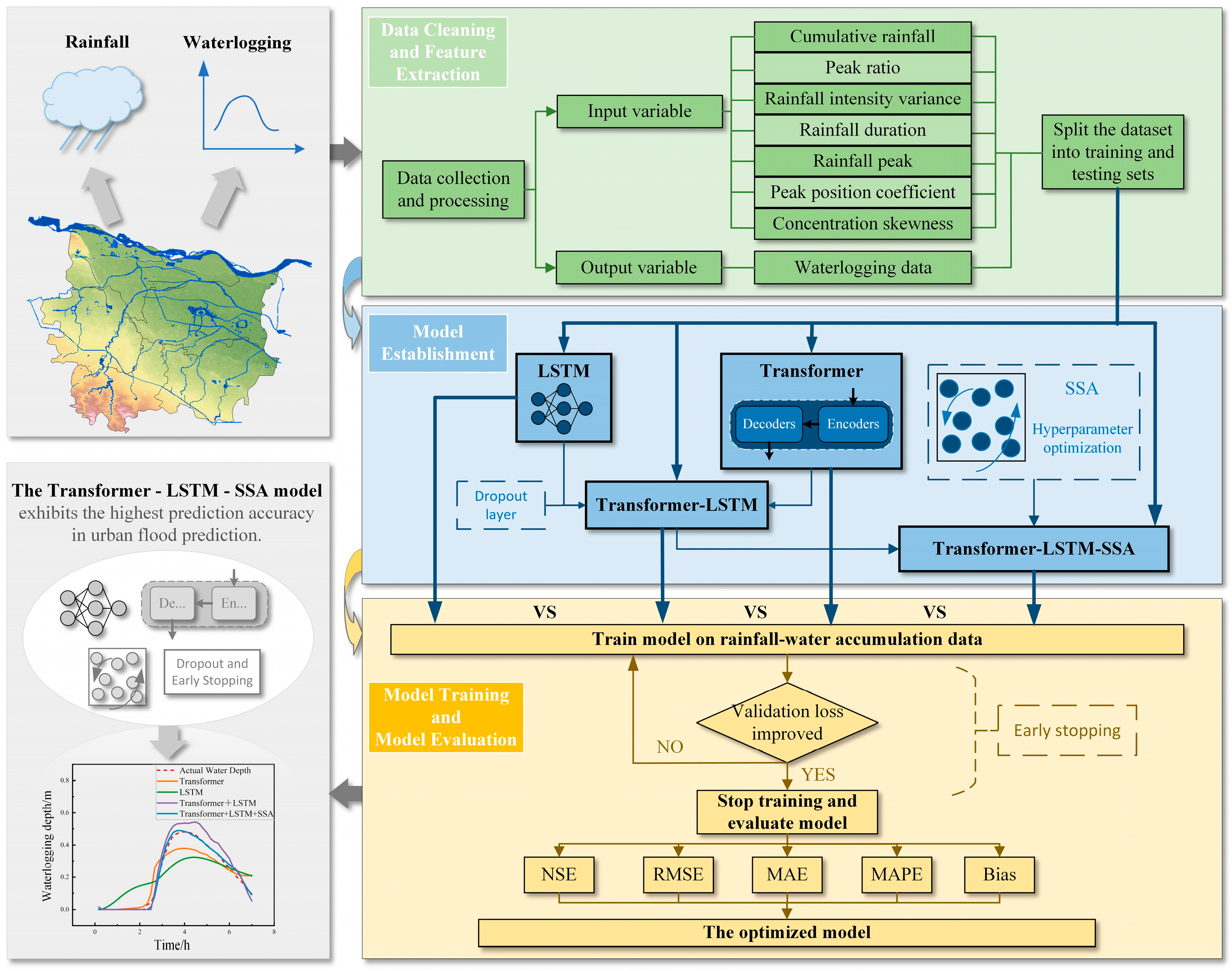
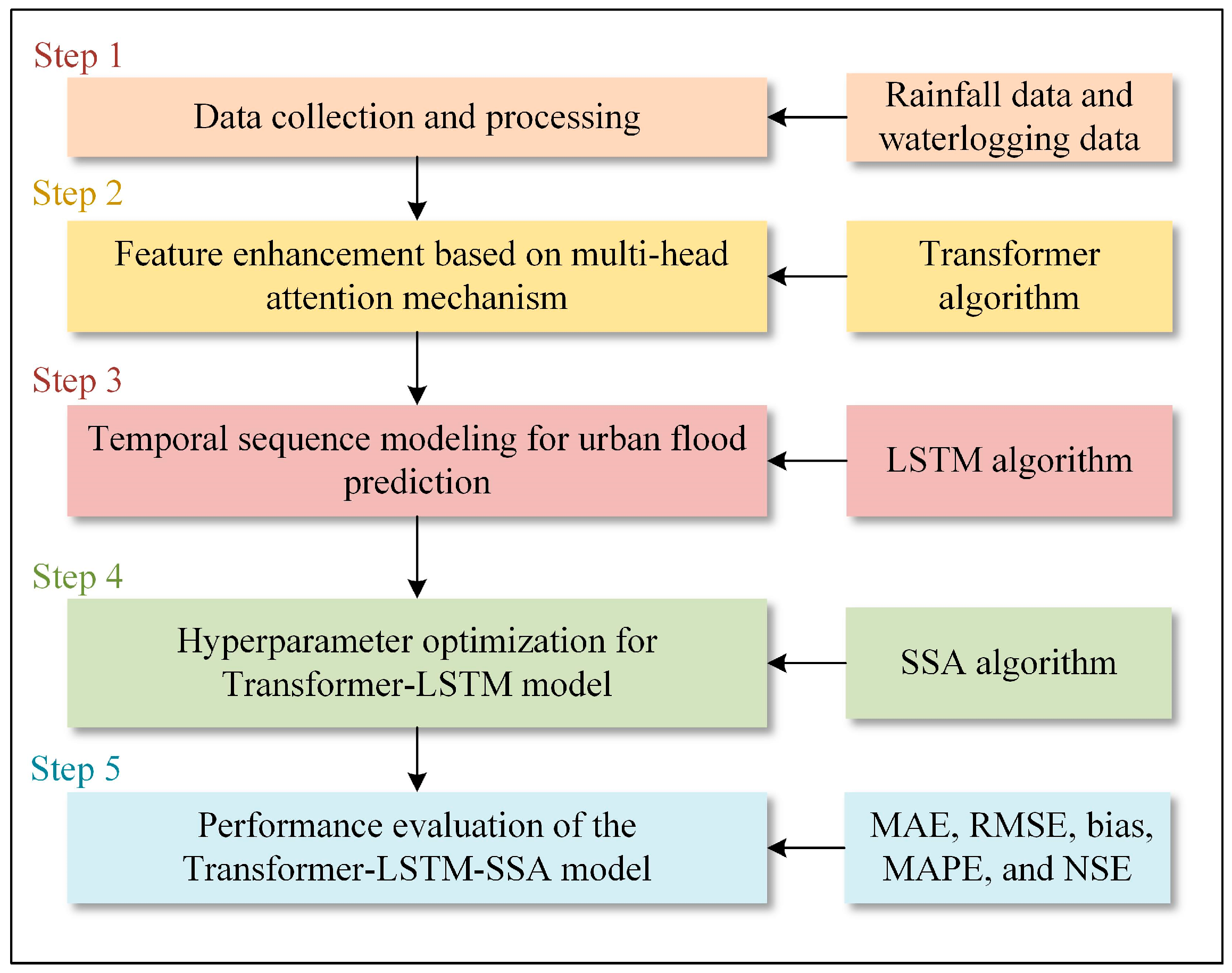
2.1. Overall Framework

This study aims to develop an urban flood prediction method based on a hybrid Transformer-LSTM-SSA model and validate its effectiveness through comparative experiments. The research framework is as follows (see Figure 1).

Step 1: Collect historical rainfall and waterlogging monitoring data from Zhengzhou City, Henan Province, China. Clean and partition the datasets to construct a sample set with multivariate input features (e.g., rainfall duration [h], rainfall peak [mm/h], cumulative rainfall [mm]) and a univariate output (waterlogging depth [m]). The data used in this study are discrete, with observations recorded at 10-minute intervals.

Step 2: Design and implement the Transformer-LSTM-SSA model innovatively. The model integrates a Transformer encoder for enhanced feature representation, an LSTM network for sequential dynamics, and the SSA for automated hyperparameter optimization. To prevent overfitting, add dropout layers to the Transformer encoder and employ an early stopping mechanism during training to dynamically adjust the number of training epochs.

Step 3: Train the proposed Transformer-LSTM-SSA model and evaluate its performance on the validation set, with LSTM, Transformer, and Transformer-LSTM models serving as comparative benchmarks to validate the effectiveness of the Transformer-LSTM-SSA hybrid model.

2.2. Urban Flood Prediction Model Based on Transformer-LSTM-SSA

This study proposes a Transformer-LSTM-SSA hybrid model. The framework first employs a Transformer encoder for feature enhancement, then utilizes LSTM layers for temporal pattern extraction. The model employs SSA to optimize hyperparameters across multiple modules, while dropout regularization in the Transformer and early stopping prevent overfitting. The framework of the Transformer-LSTM-SSA model is illustrated in Figure 2. Model performance is assessed using five metrics: Mean Absolute Error (MAE), bias, Mean Absolute Percentage Error (MAPE), Root Mean Square Error (RMSE), and the Nash–Sutcliffe Efficiency coefficient (NSE).

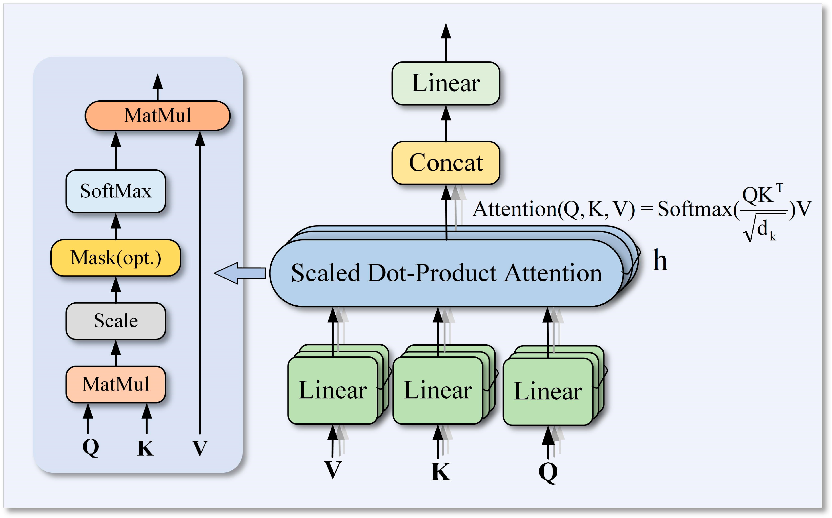
2.2.1. Transformer-LSTM Algorithm

In this study, the proposed hybrid model integrates a Transformer encoder as the feature enhancement module with the temporal modeling capability of LSTM networks, establishing a hierarchical framework for urban flood prediction (Figure 3). The input rainfall features are processed through multi-layer stacked Transformer encoders. The Transformer-derived enhanced features are further learned by the LSTM network and finally output as a one-dimensional time series through a dense layer.

(1)

Encoder-only architecture of the Transformer

The Transformer model employs self-attention mechanisms to model global dependencies in sequential data [33]. Considering the characteristics of hydrological time series data, this study extracted the encoder-only architecture of the Transformer. Dropout layers were inserted after the residual normalization and feed-forward neural network (FFN) to prevent overfitting. The encoder primarily extracts feature information through multi-head self-attention (MHSA) and a feed-forward neural network.

The multidimensional time series features $X=\left\{x_1, x_2, \dots , x_T\right\}\in {xR}^{T\times d_{\mathrm{model}}}$ are used as model inputs, where $d_{\mathrm{model}}$ denotes the dimension of the model’s hidden state and $T$ represents the time steps. The encoder consists of $N$ cascaded homogeneous layers, as described by the following equations, which are explained in detail below:

$$Q=X{W}^Q, K=X{W}^K, V=X{W}^V$$

(1)

$$\begin{array}{c}\mathrm{A}\mathrm{t}\mathrm{t}\mathrm{e}\mathrm{n}\mathrm{t}\mathrm{i}\mathrm{o}\mathrm{n}(Q,K,V)=\mathrm{S}\mathrm{o}\mathrm{f}\mathrm{t}\mathrm{m}\mathrm{a}\mathrm{x}({\displaystyle \frac{Q{K}^T}{\sqrt{d_k}}})V\end{array}$$

(2)

$${\mathrm{head}}_{\mathrm{i}}=\mathrm{Attention}(Q_i,K_i,V_i)$$

(3)

$$\mathrm{MHSA}(X)=\mathrm{Concat}({\mathrm{head}}_1,\dots ,{\mathrm{head}}_h)W^O$$

(4)

where $W^Q,W^K,W^V$ denotes Query/Key/Value projection matrices, respectively, $d_k=d_{\mathrm{model}}/h$ denotes the per-head attention dimension, and $h$ is the number of attention heads; $Q_i,K_i,V_i$ denotes head-specific projections, and $W_O$ denotes output projection.

As shown in Figure 4, in the attention mechanism, the input sequence $X$ is linearly projected into Q (Query), K (Key), and V (Value) matrices, where $W^Q,W^K,W^V$ respectively map the original features into the attention subspace (Equation (1)). Each head captures multivariate correlations via scaled dot-product computation. The attention weights are normalized through the Softmax function, and a scaling factor $\sqrt{\mathit{dk}}$ is introduced to stabilize gradients (Equation (2)). The multi-head outputs are concatenated and linearly projected to fuse multi-subspace features (Equations (3) and (4)).

$$Z=\mathrm{LayerNorm}(X+\mathrm{Dropout}(\mathrm{MHSA}(X)))$$

(5)

$$\mathrm{FFN}(Z)=\mathrm{ReLU}(Z{W}_1+b_1)W_2+b_2$$

(6)

$$Z’=\mathrm{LayerNorm}(Z+\mathrm{Dropout}(\mathrm{FFN}(Z)))$$

(7)

$$Z_{\mathrm{out}}={\mathrm{TransformerEncoder}}^N(X)$$

(8)

To enhance robustness, the self-attention output is fused with the original input via residual connections and layer normalization (Equation (5)). The FFN expands the feature space using the Rectified Linear Unit (ReLU) activation function and a hidden dimension $d_{ff}$ (Equation (6)). Notably, this study chose the ReLU activation function because it maintains model expressiveness while enabling efficient large-scale parallel computation through its simple operation [34]. These are crucial advantages for processing rainfall time series data in this study. A secondary residual normalization balances the feed-forward output with the original features again, ensuring stable gradient propagation in deep layers (Equation (7)). Finally, N cascaded encoder layers iteratively refine the features and produce high-dimensional output $Z_{\mathrm{out}}$ (Equation (8)).

(2)

LSTM temporal modeling module

Based on the high-dimensional information, this study introduced a LSTM network as the core processing module to further explore the deep temporal dependency patterns in rainfall–waterlogging time series data. LSTM, a specialized form of Recurrent Neural Network (RNN), exhibits unique advantages in handling hydrological time series data [35]. It effectively mitigates the gradient explosion problem inherent in traditional RNNs and excels in capturing dependencies within time series. The LSTM architecture comprises input gates, forget gates, and output gates, which regulate the flow of information, enabling the memory and forgetting of crucial information in the time series [36,37]. The LSTM takes the sequence features $Z_{\mathrm{out}}=\{z_1,z_2,\dots ,z_T\}$ output by the encoder as input, and its computational process is defined as follows:

$$i_t=\sigma (W_{zi}{z}_t+W_{\mathrm{hi}}{h}_{t-1}+b_i)$$

(9)

$$f_t=\sigma (W_{zf}{z}_t+W_{hf}{h}_{t-1}+b_f)$$

(10)

$$o_t=\sigma (W_{zo}{z}_t+W_{ho}{h}_{t-1}+b_O)$$

(11)

$${\tilde{c}}_t=tanh(W_{zc}{z}_t+W_{hc}{h}_{t-1}+b_c)$$

(12)

$$c_t=f_t\odot c_{t-1}+i_t\odot {\tilde{c}}_t$$

(13)

$$h_t=o_t\odot tanh(c_t)$$

(14)

Input gate $i_t$ (Equation (9)) controls the integration strength of current input features. Forget gate $f_t$ (Equation (10)) modulates the retention ratio of historical memory, influencing dependency on past information. Output gate $o_t$ (Equation (11)) governs the density of hidden state outputs, determining the significance of transmitted information. Candidate memory cell ${\tilde{c}}_{\mathrm{t}}$ (Equation (12)) updates the cell state $c_t$ (Equation (13)) by combining the forget and input gates. Finally, hidden state $h_t$ (Equation (14)) is generated from $c_t$ via the output gate. This architecture leverages the LSTM’s gating mechanisms to establish nonlinear relationships between rainfall features (extracted by the Transformer) and waterlogging time series.

2.2.2. Sparrow Search Algorithm for Hyperparameter Optimization

The configuration of model hyperparameters critically impacts the model’s expressive power and generalization performance. This study employed the SSA to systematically optimize hyperparameters. As illustrated in Figure 5, SSA initializes a population of random hyperparameter combinations and iteratively adjusts them to minimize the objective function. During each iteration, SSA simulates the foraging and vigilance behaviors of sparrows, constructing an “Explorer-Follower-Vigilante” search mechanism: Explorers generate diverse hyperparameter combinations and evaluate their fitness. Followers update their positions based on the best solutions identified by explorers. Vigilantes monitor global anomalies and adjust search strategies to avoid local optima. The mathematical formulation of SSA is detailed in Equations (15)–(17).

Explorers Position Update:

$$x_i^{t+1}=\left\{\begin{array}{c}{x}_i^t·\exp \left(-{\displaystyle \frac{i}{\alpha · {\mathrm{iter}}_{\max }}}\right),R_2<ST\\ x_i^t+Q·L,R_2\ge ST\end{array}\right.$$

(15)

Here, $R_2$ and $ST$ represent the safety threshold and alert threshold, respectively. When $R_2<ST$, sparrows perform global exploration for foraging; when $R_2\ge \mathrm{ST}$, they engage in random walks following a normal distribution.

Followers Position Update:

$$x_i^{t+1}=\left\{\begin{array}{c}Q\cdot \exp \left({\displaystyle \frac{x_{\mathrm{worst}}^t-x_i^t}{i^2}}\right),i>n/2\\ x_p^t+\left|x_i^t-x_p^t\right|\cdot A^{+}\cdot L, \mathrm{o}\mathrm{t}\mathrm{h}\mathrm{e}\mathrm{r}\mathrm{w}\mathrm{i}\mathrm{s}\mathrm{e}\end{array}\right.$$

(16)

When $\mathrm{i}>n/2$, sparrows with lower fitness levels seek more food resources. Otherwise, they search randomly near the current optimal position.

Vigilantes Position Update:

$$x_i^{t+1}=\left\{\begin{array}{c}{x}_{\mathrm{best}}^t+\beta \cdot \left|x_i^t-x_{\mathrm{best}}^t\right|,{ f}_i\ne f_g\\ x_i^t+K\left({\displaystyle \frac{x_i^t-x_{\mathrm{worst}}^t}{\left|f_i-f_w\right|+\epsilon }}\right),f_i=f_g\end{array}\right.$$

(17)

When ${ f}_i\ne f_g$, the sparrow is at the edge of the population, prompting it to move toward the best position. When $f_i=f_g$, the sparrow is in a dangerous position.

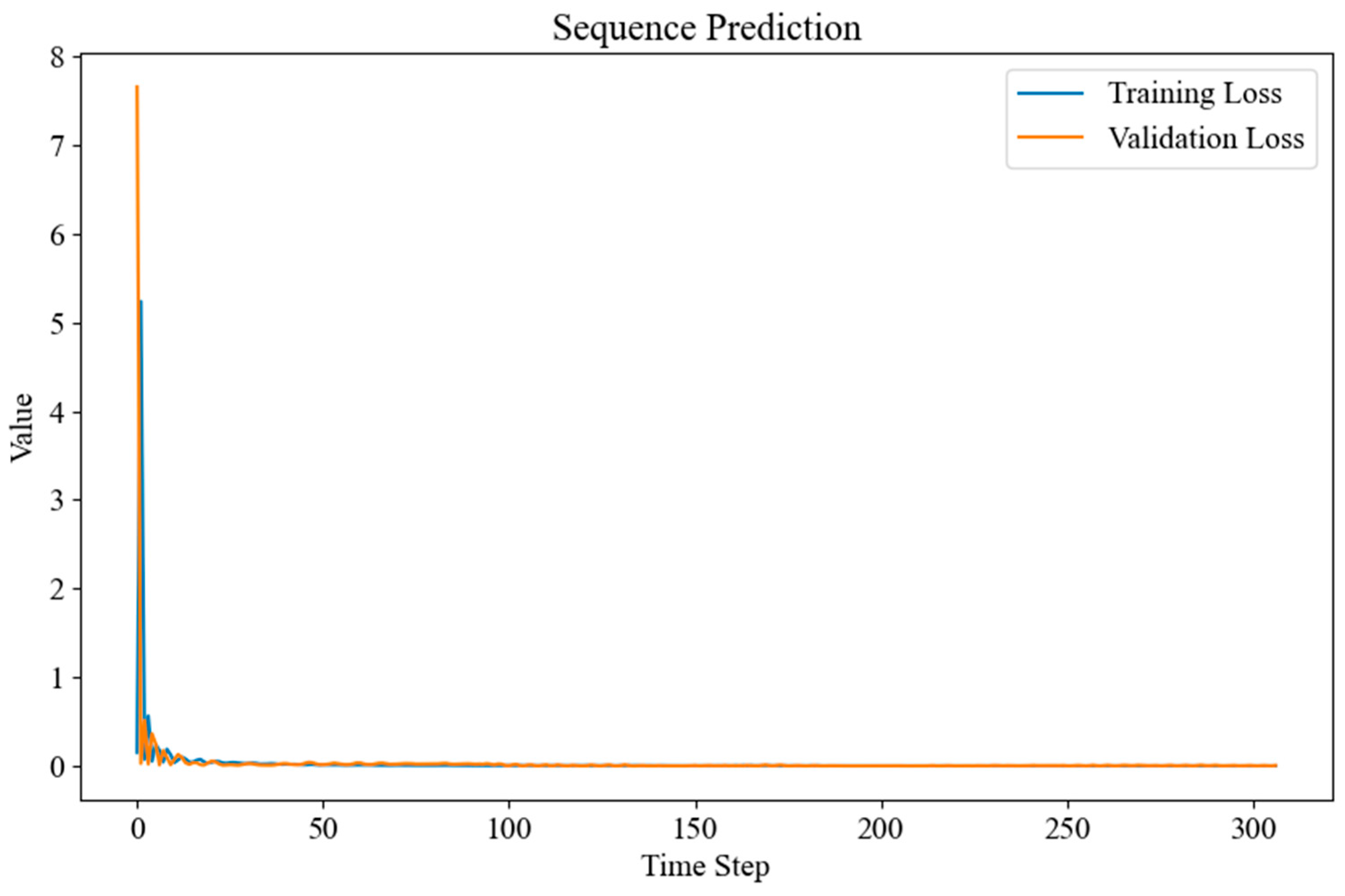
2.2.3. Overfitting Control of the Transformer-LSTM-SSA Model

The integration of multiple components in the Transformer-LSTM-SSA model significantly increases its complexity, rendering it susceptible to overfitting. To mitigate this issue, a dual regularization strategy was employed. Specifically, dropout was applied to the Transformer encoder, while an early stopping mechanism was introduced into the entire model.

(1) Dropout randomly drops neurons during training with a certain probability, thereby reducing inter-neuron dependencies and enabling the model to learn more robust representations.

(2) The core idea of early stopping is to evaluate the model’s performance on the validation set after each training iteration. As training progresses, the training loss typically decreases, while the validation loss may start to increase after reaching a minimum, indicating overfitting. A sliding window approach is used to track the validation loss. If the validation loss decreases by less than a threshold ϵ over K consecutive epochs, the optimal weights ${\theta }^{\ast }={\mathrm{argmin}}_{\theta }{L}_{\mathrm{val}}$ are retained, as shown in Equation (18):

$$\exists k\in \{1,\dots ,K\}, L_{\mathrm{val}}^{(t-k)}-L_{\mathrm{val}}^{\left(t\right)}<ϵ$$

(18)

where $L_{\mathrm{val}}$ indicates the validation loss calculated on the dataset, K indicates the number of consecutive epochs, ϵ denotes the minimum required loss improvement threshold, $\theta$ corresponds to model parameters, and ${\theta }^{\ast }$ corresponds to the optimal parameters that achieve the minimal validation loss.

2.2.4. Model Performance Evaluation

To evaluate the model’s performance in predicting flood time series, this study compared it with the Transformer, LSTM, and Transformer-LSTM models using the following metrics: Mean Absolute Error (MAE), Root Mean Squared Error (RMSE), Mean Absolute Percentage Error (MAPE), bias, and Nash–Sutcliffe Efficiency (NSE). Lower MAE, RMSE, and MAPE values, bias closer to zero, and higher NSE values indicate greater prediction accuracy. The criteria are defined as follows:

$$\begin{array}{c}RMSE=\sqrt{{\displaystyle \frac{1}{n}}{\displaystyle \sum _{i=1}^n}{(o_i-y_i)}^2}\end{array}$$

(19)

$$\begin{array}{c}MAE={\displaystyle \frac{1}{n}}{\displaystyle \sum _{i=1}^n}\left|o_i-y_i\right|\end{array}$$

(20)

$$\begin{array}{c}NSE=1-{\displaystyle \frac{\sum _{i=1}^n{(o_i-y_i)}^2}{\sum _{i=1}^n{(y_i-{\overline{y}}_i)}^2}}\end{array}$$

(21)

$$\begin{array}{c}MSPE={\displaystyle \frac{100\%}{n}}{\displaystyle \sum _{n=1}^n}{\displaystyle \frac{\left|o_i-y_i\right|}{o_i}}\end{array}$$

(22)

$$\begin{array}{c}Bias={\displaystyle \frac{1}{n}}{\displaystyle \sum _{i=1}^n}\left(o_i-y_i\right)\end{array}$$

(23)

where $o_i$ is the actual value, $y_i$ is the predicted value, ${\overline{y}}_i$ is the mean of the actual values, and n is the sample size.

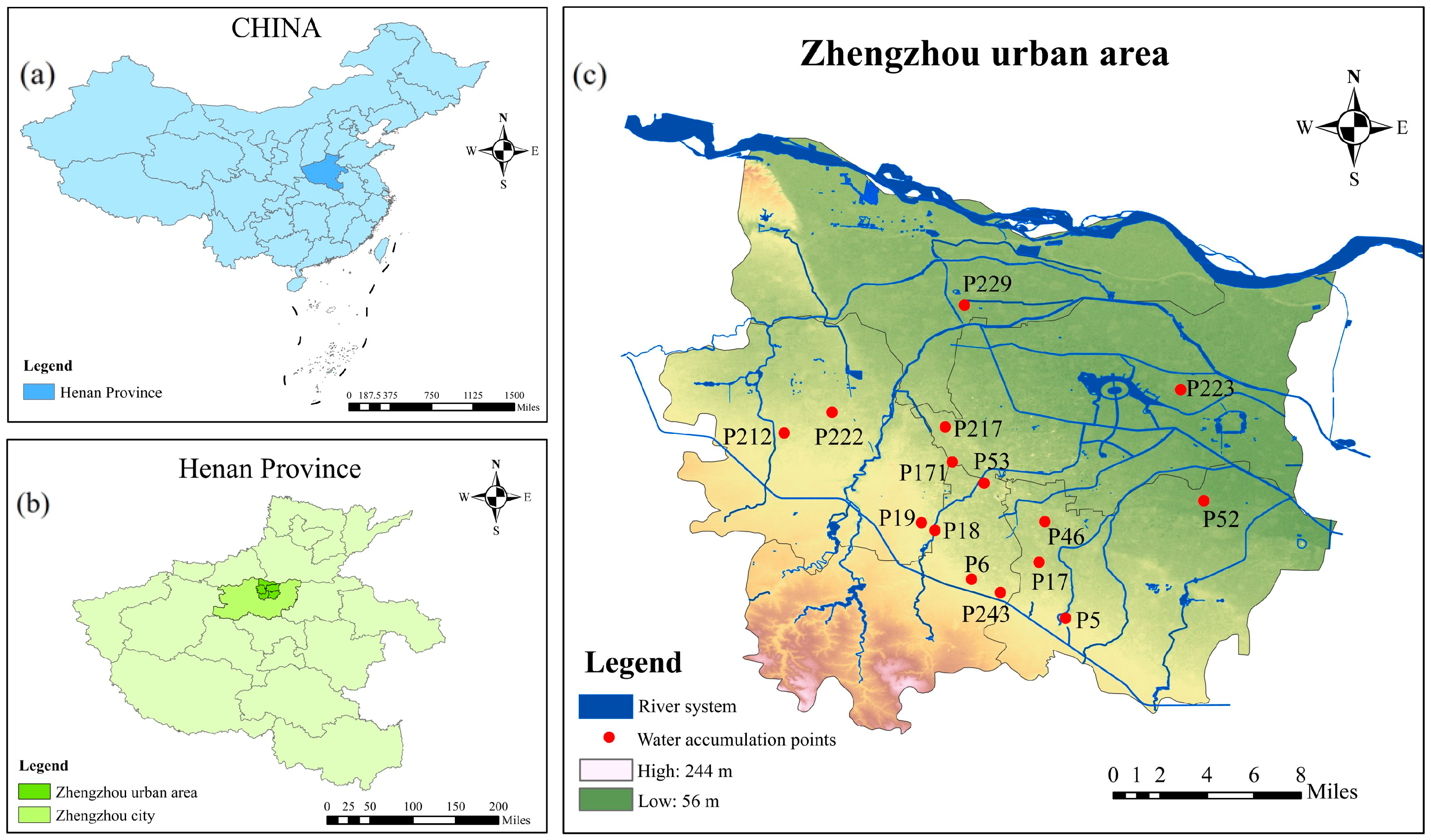
2.3. Study Area and Data

Considering data availability, this study focused on Zhengzhou City, Henan Province, China (112°42′–114°13′ E, 34°16′–34°58′ N). As the provincial capital of Henan, Zhengzhou covers an area of 7568.0 km² and is located in the middle and lower reaches of the Yellow River. The terrain slopes from west to east, causing rapid runoff from the western mountainous areas to the eastern urban plains during heavy rainfall events [38]. This distinct topography combined with rapid urbanization results in exceptional flood vulnerability. These characteristics result in particularly rapid and sensitive water accumulation responses to rainfall inputs, with ponding depth fluctuations showing heightened dependence on different rainfall characteristics [39].

Zhengzhou has a temperate monsoon climate with unevenly distributed precipitation. Winters are cold with minimal snowfall, while summers are hot and rainy. The average annual rainfall is approximately 640.9 mm, with frequent extreme rainfall events [40,41]. For instance, the “7·20” extreme rainfall event in 2021 recorded an hourly precipitation of 201.9 mm. This event inundated 10.29% of Zhengzhou’s total area and affected 7.55% of its population [42,43].

Rainfall data were provided by the Zhengzhou Meteorological Bureau. This study selected 16 rainfall events from 2014 to 2018 as sample data. Using the Kriging spatial interpolation method [44], rainfall data from different gauges were mapped to 15 waterlogging points to obtain corresponding rainfall processes. Waterlogging data were obtained from the Zhengzhou Urban Management Bureau [45]. The study utilized waterlogging process data from 15 waterlogging points, each with a duration of 420 min. The locations of water accumulation points are shown in Figure 6.

The raw data consist of rainfall and waterlogging processes at different waterlogging points. Since Transformer and LSTM models cannot directly process these raw sequences, the data were transformed into feature indicators suitable for model training [46]. Using an equidistant segmentation and recombination approach, the complete rainfall and waterlogging processes were divided into sub-processes, and corresponding feature values were calculated for each subset. To ensure interpretability and align with hydrological principles, seven rainfall features significantly influencing waterlogging depth in Zhengzhou were selected based on prior research: rainfall duration, cumulative rainfall, peak rainfall intensity, peak ratio, rainfall intensity variance, peak position coefficient, and concentration skewness [47].

3. Results

3.1. Urban Flood Prediction Model Based on Transformer-LSTM Algorithm

In this study, rainfall feature data were mapped into a complex high-dimensional space through an embedding layer, with positional encoding incorporated to capture sequential information. These representations were processed by a multi-layer Transformer encoder, with dropout regularization enhancing generalization. The encoder outputs high-dimensional information encapsulating multi-level rainfall features. The LSTM network processes the high-dimensional output from the Transformer encoder, leveraging its gated mechanism to model long-term and short-term dependencies in the time series. The final output is a predicted sequence of waterlogging depths at the target points.

The dataset was partitioned into training (12 rainfall events) and validation (4 rainfall events) sets at a 3:1 ratio across all 15 waterlogging points. During training, the Mean Squared Error (MSE) is used as the loss function to minimize the difference between predicted and actual waterlogging depths. The Adam optimizer dynamically adjusts the learning rate to accelerate convergence. Early stopping is employed to prevent overfitting, halting training if the validation loss does not improve for 100 consecutive epochs and retaining the best-performing model.

Experimental results demonstrate that the Transformer-LSTM model effectively captures the complex nonlinear relationships between rainfall features and waterlogging responses, achieving high predictive accuracy on the validation set. The model achieves an average NSE of 0.942, MAPE of 30.24%, bias of 0.007 m, RMSE of 0.049 m, and MAE of 0.038 m. To further analyze model performance, the validation results were further analyzed by event type, with metrics averaged across 15 monitoring points for each of the four rainfall events.

As shown in

Table 1. The average metrics of the Transformer-LSTM model under different rainfall events in the validation set.

Rainfall Events	Rainfall 1	Rainfall 2	Rainfall 3	Rainfall 4	Mean
RMSE (m)	0.052	0.046	0.043	0.056	0.049
MAE (m)	0.043	0.033	0.032	0.045	0.038
MAPE (%)	20.60	25.15	30.77	44.44	30.24
Bias (m)	0.007	0.008	−0.003	0.017	0.007
NSE	0.936	0.947	0.963	0.922	0.942

, the Transformer-LSTM model exhibits relatively lower performance for the fourth rainfall event, with an NSE of 0.922, 2% below the overall average. Two potential causes explain this discrepancy: (1) As shown in Figure 7, the fourth rainfall event’s feature distribution significantly differs from other rainfall events of the training set. This rainfall event, characterized by both high peak intensity and delayed peak timing, poses the most severe challenges to urban flood drainage. This inconsistency in distribution may lead to the model’s failure to adequately learn the rainfall–waterlogging response mechanism of this event during training, limiting the model’s ability to generalize. (2) Key hyperparameters of the model (the number of attention heads, encoder layers, and hidden units, etc.) may not be optimally configured, restricting the model’s capacity to capture complex nonlinear relationships. To address hyperparameter optimization, this study introduced a systematic parameter search algorithm to explore optimal configurations.

3.2. Hyperparameter Optimization Based on SSA

To further enhance the predictive performance of the Transformer-LSTM model, this study employed SSA to optimize its key hyperparameters. The selected hyperparameters for optimization are the number of Transformer encoders, the number of attention heads in the multi-head attention mechanism, the number of hidden layer units in the Transformer encoder, the number of hidden layer units in the LSTM, and the dropout rate. Although the SSA alleviates local convergence through its vigilance mechanism, it remains susceptible to premature convergence when optimizing multivariate functions [48]. To mitigate this issue, this study configured a reasonable population size and a relatively large number of iterations in the SSA algorithm. The SSA was configured with a population size of 20 and a maximum of 50 iterations. During the optimization process, SSA iteratively updates the positions of the sparrow individuals, gradually converging toward the optimal hyperparameter combination.

Figure 8 illustrates the evolution of the fitness function during the iterations. The curve demonstrates that SSA effectively minimizes the objective function value within the first few iterations. Specifically, the validation set NSE increased from 0.962 to 0.977 in the second iteration and further to 0.989 in the third iteration, after which the fitness function stabilized. This indicates that SSA achieves rapid convergence to a global optimum within a small number of iterations, significantly reducing computational complexity and saving time costs.

Table 2. Optimization range and optimal hyperparameters of SSA.

Number	Attention Heads	Encoder Layers	Hidden-Layers 1	Dropout Rate	Hidden-Layers 2
Range	1–10	1–10	64,128,256	0–0.5	64,128,256
Optimized parameters	6	3	128	0.16	256

Note: Hidden-layers 1 and Hidden-layers 2 denote the number of hidden units in the Transformer and LSTM layers, respectively.

shows the optimization range and optimal hyperparameters of SSA. The final optimized hyperparameters for the Transformer-LSTM-SSA model include 6 attention heads, 3 Transformer encoders, 128 hidden layer units in the Transformer encoder, 256 hidden layer units in the LSTM, and a dropout rate of 0.16.

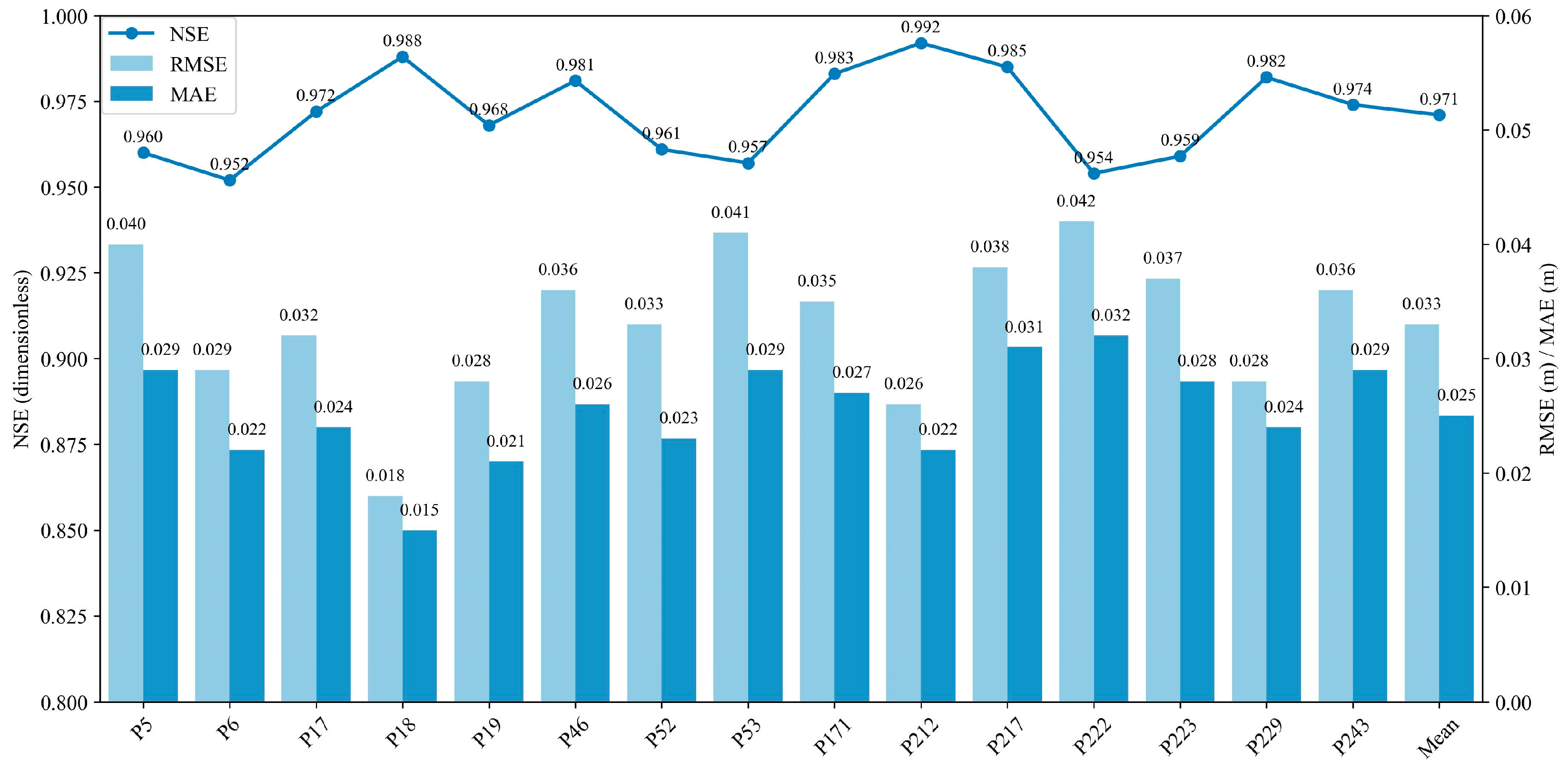
3.3. Performance Evaluation of Transformer-LSTM-SSA Model for Urban Flood Prediction

The Transformer-LSTM model was retrained using the hyperparameters optimized by the SSA, and its performance was comprehensively evaluated. Figure 9 shows the average metrics of the Transformer-LSTM-SSA model across four rainfall events in the validation set at different waterlogging points. The results show that the Transformer-LSTM- SSA model achieves an overall average NSE of 0.971, RMSE of 0.033 m, and MAE of 0.025 m across all validation sets. The NSE values for all waterlogging points exceed 0.90, while RMSE and MAE values are consistently below 0.05 m, indicating minimal deviation between predicted and actual values. The model accurately captures the overall trend of water depth changes and demonstrates high stability, providing reliable predictions across different geographical locations. Among the 15 waterlogging points, 6 points achieve NSE values above 0.98, indicating near-perfect alignment between predicted and actual results at over one-third of the points.

To further illustrate the model’s performance, the waterlogging point with the lowest prediction accuracy was selected: P6, which has the lowest NSE value (0.952), and P222, which has the highest RMSE (0.042 m) and MAE (0.032 m) values. This study attributes the relatively poor simulation accuracy of the model at this location to the higher density of drainage networks and the steeper surface slope in this area, which may hinder the model’s ability to effectively capture the rainfall–waterlogging response relationship. As shown in Figure 10 and Figure 11, the predicted versus actual water depth curves for this point under four rainfall events from the validation set are compared. The results demonstrate the model’s exceptional ability to capture peak water depths, with predicted peaks closely aligning with actual peaks. This highlights the model’s high accuracy, robustness, and stability across diverse geographical locations and rainfall events.

4. Discussion

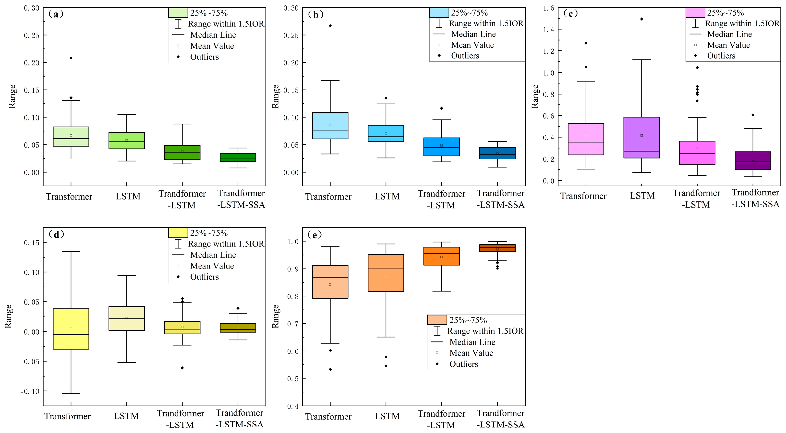
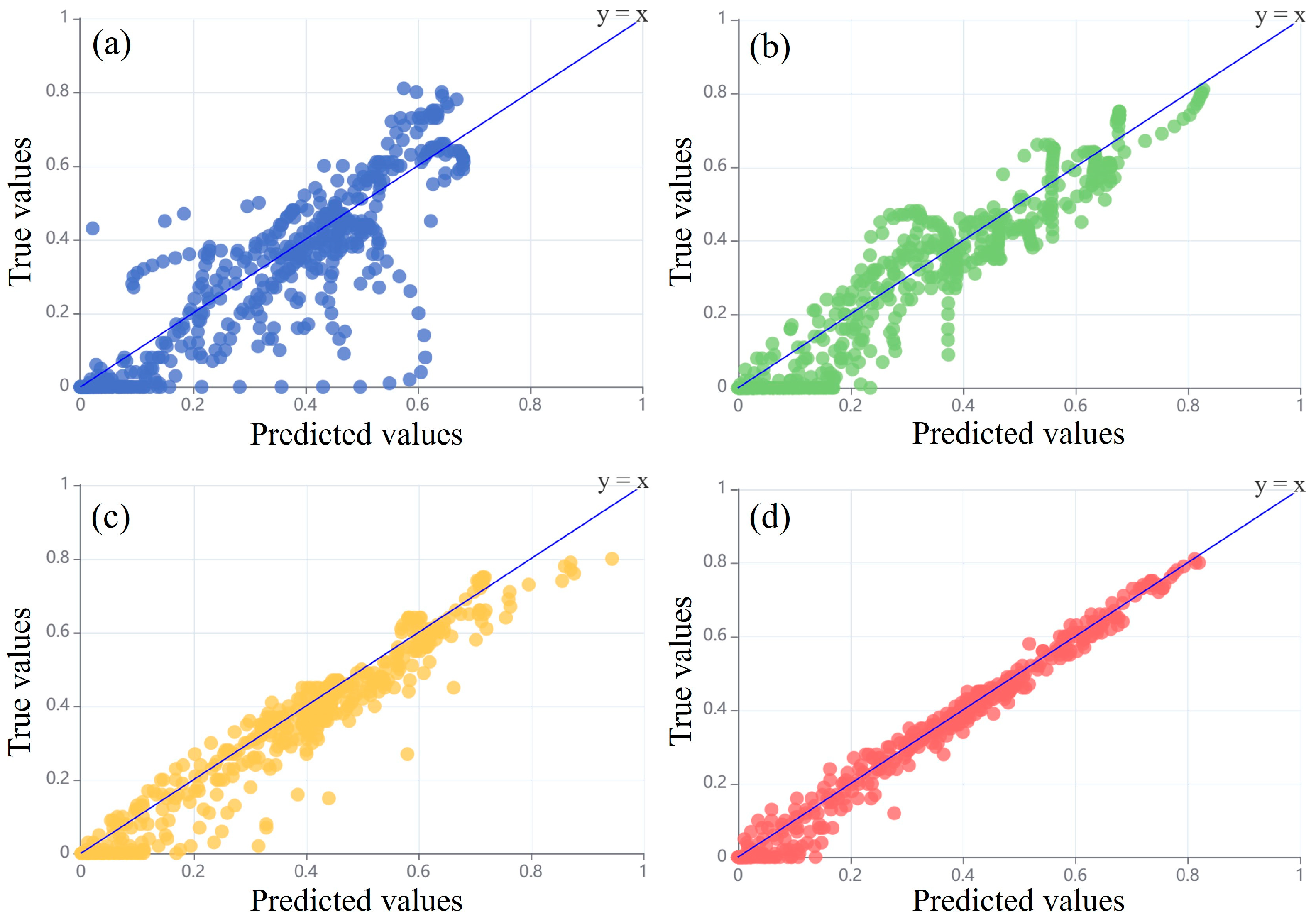
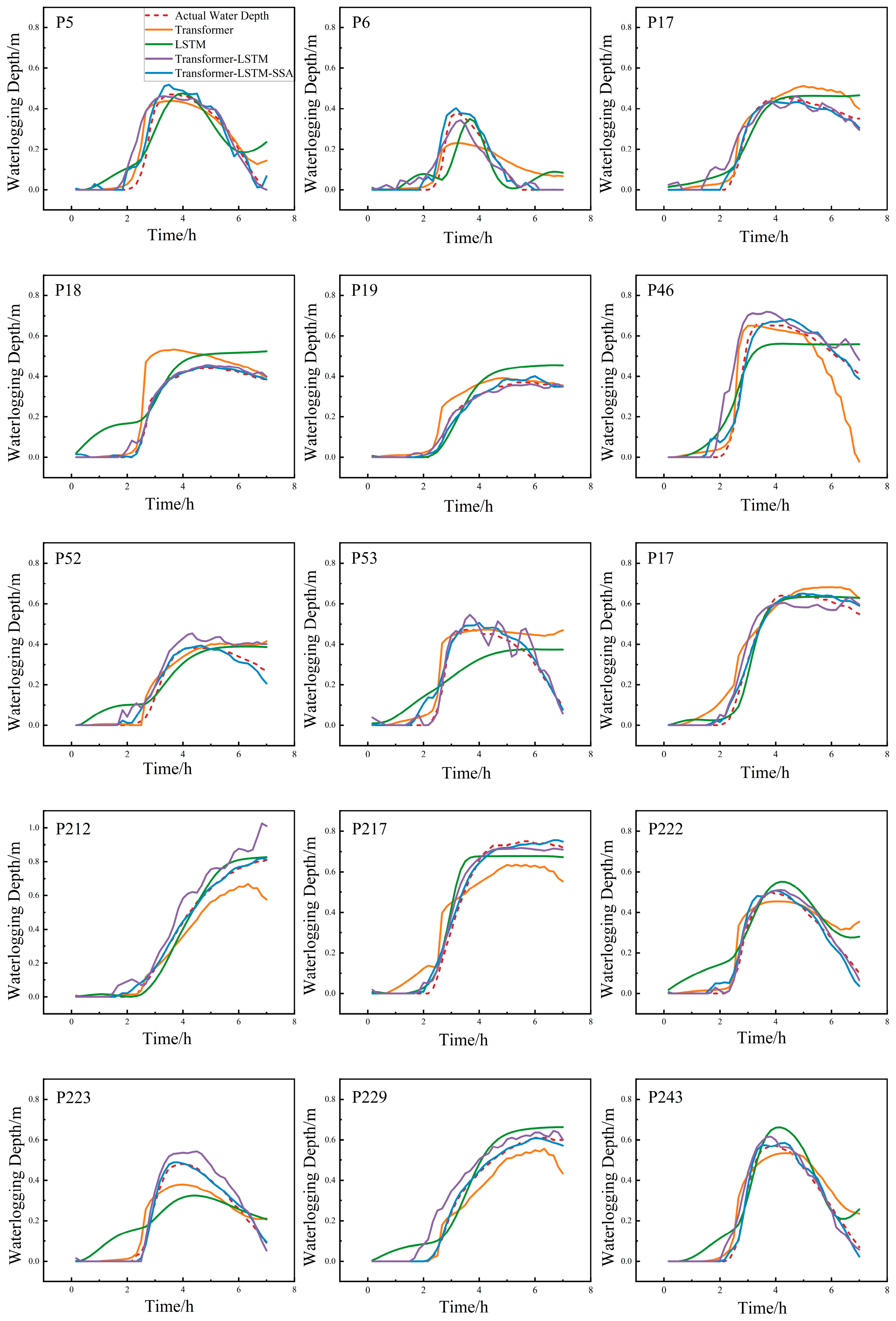
4.1. Comparative Performance of Different Models for Urban Flood Prediction

Based on average evaluation metrics on the validation set, this study compared the predictive performance of four models: Transformer-LSTM-SSA, Transformer, LSTM, and Transformer-LSTM. The results are summarized in

Table 3. Comparison of average evaluation metrics across models.

Model	Transformer	LSTM	Transformer-LSTM	Transformer-LSTM-SSA
RMSE (m)	0.086	0.070	0.049	0.033
MAE (m)	0.066	0.058	0.038	0.025
MAPE (%)	41.04	41.55	30.24	19.35
Bias (m)	0.004	0.022	0.007	0.005
NSE	0.842	0.870	0.942	0.971

.

The comparison reveals that the Transformer-LSTM-SSA model significantly outperforms the others across all metrics. The Transformer model exhibits the lowest performance, with an NSE of only 0.842, likely due to its original design for language processing tasks, which limits its effectiveness in regression tasks. In contrast, the LSTM model shows improved performance, achieving an NSE of 0.870, consistent with its strength in capturing long-term dependencies in time series data. However, the standalone LSTM model still struggles to meet the high precision requirements of complex multivariate regression tasks.

The Transformer-LSTM model demonstrates a substantial performance improvement. Compared to the Transformer model, its RMSE decreases by 0.037 m, MAE by 0.028 m, MAPE by 10.8%, and NSE increases by 10.0%. Relative to the LSTM model, the RMSE of the Transformer-LSTM model decreases by 0.021 m, MAE by 0.020 m, bias by 0.015 m, MAPE by 11.31%, and NSE increases by 7.2%. This enhancement demonstrates the superiority of the hybrid model, indicating that the Transformer-LSTM architecture effectively captures dynamic interdependencies among rainfall characteristics and accurately models rainfall–flooding response processes. Further optimization using SSA leads to another significant improvement in the Transformer-LSTM-SSA model. Compared to the Transformer-LSTM model, its RMSE decreases by 0.016 m (a reduction of 32.6%), MAE by 0.013 m (a reduction of 34.2%), bias by 0.002 m (a reduction of 28.5%), MAPE by 10.89%, and NSE increases by 2.9%. These results demonstrate that the Sparrow Search Algorithm effectively enhances the performance of the Transformer-LSTM hybrid model, achieving the highest levels of prediction accuracy and stability.

Figure 12 displays boxplots of the metric distributions for different models. The Transformer-LSTM-SSA model exhibits lower dispersion and better medians than the other models, demonstrating more stable performance. In contrast, the Transformer and LSTM display greater dispersion. Especially for the Transformer model, the variability is higher, and the RMSE is greater, indicating unstable performance. Notably, the Transformer model exhibits significant fluctuations in bias values, indicating unstable model performance. However, its uniformly distributed positive and negative bias values cancel each other out during averaging, resulting in a potentially misleading mean bias measurement. This explains why the Transformer model demonstrates a lower mean bias than the Transformer-LSTM-SSA model, despite its poorer overall stability and higher prediction errors.

This study compared the predicted versus actual values at each time step across the different models (as shown in Figure 13). The scatter plot for the Transformer-LSTM-SSA model is tightly clustered around the diagonal, with the least dispersion, indicating a high degree of agreement between predicted and actual values. The Transformer-LSTM model follows, though it exhibits slightly larger deviations in the high-value region, likely due to its limited ability to capture extreme values. The LSTM model ranks third, while the Transformer model shows the highest dispersion in its scatter plot, reflecting the poorest predictive performance.

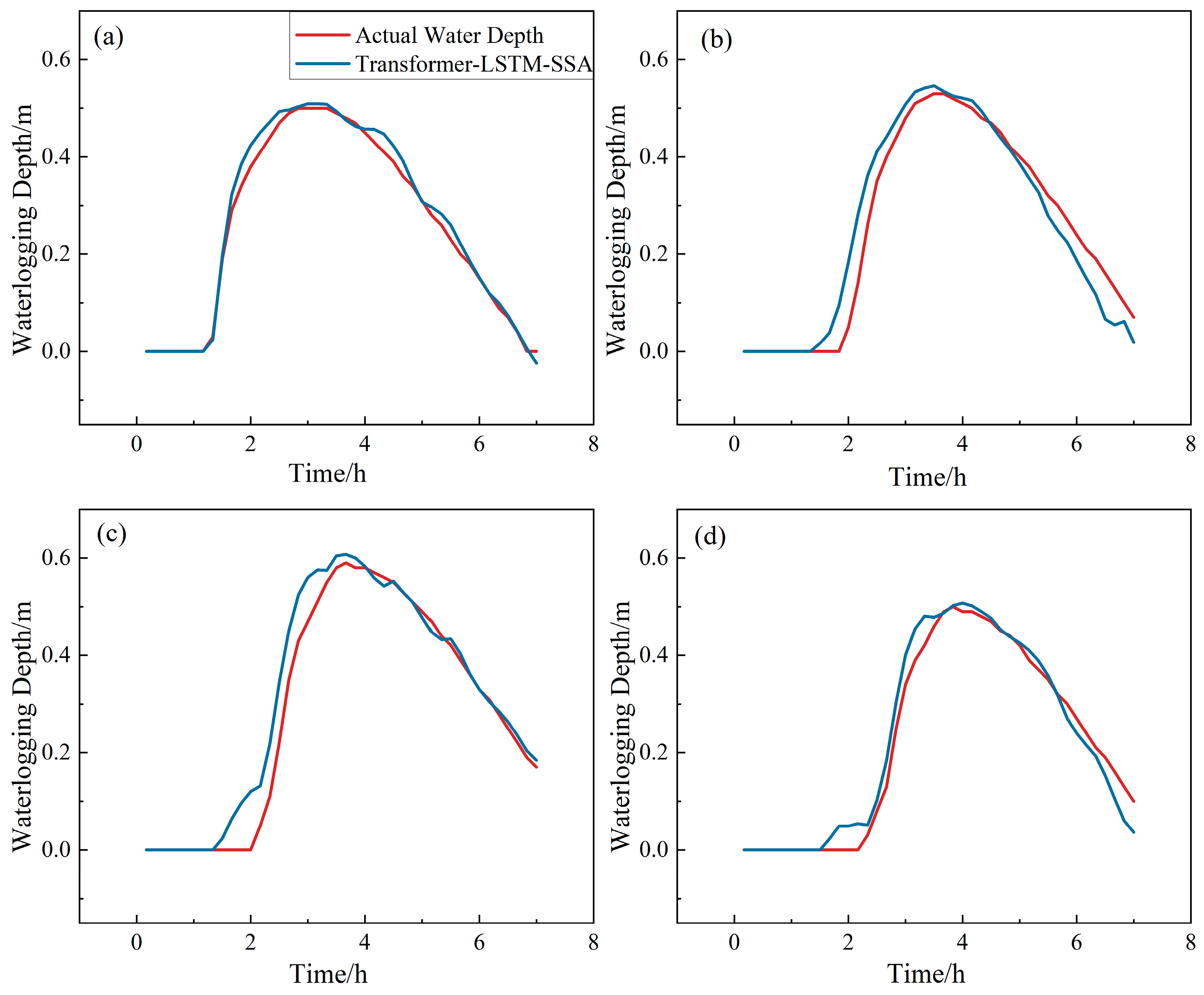
4.2. Waterlogging Process Prediction of Different Models

This study visualized the predicted waterlogging processes of different models at various waterlogging points (as shown in Figure 14). The Transformer-LSTM-SSA model accurately captures the trends of waterlogging changes and significantly outperforms other models in predicting peak waterlogging levels. In contrast, the Transformer-LSTM model exhibits less smooth prediction curves, with jagged patterns observed at some points (e.g., P53 and P212 in Figure 14). This may be attributed to the limitations of the Transformer component in handling local details, combined with the increased complexity introduced by the LSTM component, which slightly compromises the model’s ability to process fine-grained features. The standalone Transformer and LSTM models show unstable predictions, with significant deviations at some waterlogging points.

Overall, the comparative results are highly satisfactory, demonstrating that the Transformer-LSTM-SSA model can accurately predict maximum waterlogging levels, as well as the timing of water rise and recession. The comparison of waterlogging process time series across different points further confirms the model’s ability to precisely simulate the temporal evolution of floodwater levels in diverse regions.

4.3. Impact of Overfitting Control on Prediction Efficiency

Overfitting can lead to excellent performance on the training set but poor generalization on the validation set. The combination of dropout and early stopping mechanisms significantly enhances the Transformer-LSTM-SSA model’s ability to prevent overfitting. Dropout improves the model’s feature extraction and generalization capabilities by randomly deactivating neurons in the Transformer during training. Early stopping dynamically monitors the validation loss to ensure training halts at the optimal point, avoiding underfitting due to insufficient training epochs and preventing a decline in model accuracy caused by excessive training.

The integration of these two regularization techniques stabilizes the loss reduction during training and allows for early termination when the model is sufficiently trained, effectively reducing training time. As illustrated in Figure 15 for waterlogging point P17, the maximum training epochs are set to 600. While the training loss continues to decrease steadily, the validation loss begins to rise after the 207th epoch. The early stopping mechanism intervenes to terminate training at the 307th epoch, improving training efficiency by 48.83% for this specific waterlogging point.

4.4. Limitations and Future Perspectives

Although the Transformer-LSTM-SSA model developed in this study has demonstrated promising performance in urban flood prediction, several limitations remain. From a data perspective, the dataset does not fully incorporate multi-source data, such as urban land use types and drainage network information. This may result in an incomplete representation of influencing factors. Future research should focus on expanding the dataset by collecting multi-scale and multi-source data, and developing effective data fusion techniques. From a model perspective, the complex architecture of the model limits its interpretability, making it difficult to uncover the physical processes and causal relationships between rainfall characteristics and waterlogging responses. This restricts the model’s deep application in urban flood management. Future research should aim to develop more efficient and lightweight model architectures while enhancing model interpretability such as SHAP value analysis and visualization of Transformer attention weight maps to reveal the physical basis of model decisions.

In the future, this model can integrate Geographic Information Systems (GISs) to enable real-time monitoring and early warning. It can be applied to local government emergency management by predicting the locations and severity of waterlogging points in advance during heavy rainfall events, thereby improving emergency response efficiency. Additionally, it can support urban flood mitigation through applications in spatial planning, drainage system optimization, and critical infrastructure management.

5. Conclusions

This study proposed an urban flood prediction method based on a Transformer-LSTM-SSA hybrid model, which integrates the global feature extraction capability of the Transformer encoder, the temporal modeling ability of LSTM, and the hyperparameter optimization mechanism of the Sparrow Search Algorithm, along with an overfitting control module, to achieve accurate and real-time flood simulation in urbanized areas.

Using Zhengzhou City as the study area, four deep learning-based flood inundation prediction models were constructed—Transformer, LSTM, Transformer-LSTM, and Transformer-LSTM-SSA—to validate the superiority of the Transformer-LSTM-SSA model. Experimental results demonstrate that the Transformer-LSTM-SSA model achieves satisfactory performance in predicting waterlogging depth time series, outperforming the other models with high prediction accuracy and generalization capability. On the validation set, the model achieved an average Nash–Sutcliffe Efficiency (NSE) of 0.971, a Mean Absolute Percentage Error (MAPE) of 19.35%, a bias of 0.005 m, a Root Mean Square Error (RMSE) of 0.033 m, and a Mean Absolute Error (MAE) of 0.025 m. The model exhibited high precision and strong stability across all waterlogging points in the dataset, with exceptional performance in capturing peak waterlogging levels. The Transformer-LSTM model followed in performance, with the LSTM model ranking third, and the Transformer model showing the poorest performance.

This study highlights the innovative nature of the Transformer-LSTM-SSA hybrid model. By integrating the strengths of multiple models, it overcomes the limitations of traditional single models in handling complex urban flood data, providing new insights and methodologies for the field of urban flood prediction.

References

1. Kundzewicz, Z.W.; Kanae, S.; Seneviratne, S.I.; Handmer, J.; Nicholls, N.; Peduzzi, P.; Mechler, R.; Bouwer, L.M.; Arnell, N.; Mach, K.; et al. Flood risk and climate change: Global and regional perspectives. Hydrol. Sci. J. 2013, 59, 1–28. [Google Scholar] [CrossRef]
2. Hammond, M.J.; Chen, A.S.; Djordjević, S.; Butler, D.; Mark, O. Urban flood impact assessment: A state-of-the-art review. Urban Water J. 2013, 12, 14–29. [Google Scholar] [CrossRef]
3. Guan, X.; Yu, F.; Xu, H.; Li, C.; Guan, Y. Flood risk assessment of urban metro system using random forest algorithm and triangular fuzzy number based analytical hierarchy process approach. Sustain. Cities Soc. 2024, 109, 105546. [Google Scholar] [CrossRef]
4. Wang, W.; Yuan, X. Climate change and La Niña increase the likelihood of the ‘7·20’ extraordinary typhoon-rainstorm in Zhengzhou, China. Int. J. Climatol. 2024, 44, 1355–1370. [Google Scholar] [CrossRef]
5. Xu, T.; Xie, Z.; Zhao, F.; Li, Y.; Yang, S.; Zhang, Y.; Yin, S.; Chen, S.; Li, X.; Zhao, S.; et al. Permeability control and flood risk assessment of urban underlying surface: A case study of Runcheng south area, Kunming. Nat. Hazards 2022, 111, 661–686. [Google Scholar] [CrossRef]
6. Teng, J.; Jakeman, A.J.; Vaze, J.; Croke, B.F.; Dutta, D.; Kim, S. Flood inundation modelling: A review of methods, recent advances and uncertainty analysis. Environ. Model. Softw. 2017, 90, 201–216. [Google Scholar] [CrossRef]
7. Neal, J.; Schumann, G.; Fewtrell, T.; Budimir, M.; Bates, P.; Mason, D. Evaluating a new LISFLOOD-FP formulation with data from the summer 2007 floods in Tewkesbury, UK. J. Flood Risk Manag. 2011, 4, 88–95. [Google Scholar] [CrossRef]
8. Alfieri, L.; Salamon, P.; Pappenberger, F.; Wetterhall, F.; Thielen, J. Operational early warning systems for water-related hazards in Europe. Environ. Sci. Policy. 2012, 21, 35–49. [Google Scholar] [CrossRef]
9. Lei, X.; Chen, W.; Panahi, M.; Falah, F.; Rahmati, O.; Uuemaa, E.; Kalantari, Z.; Ferreira, C.S.S.; Rezaie, F.; Tiefenbacher, J.P.; et al. Urban flood modeling using deep-learning approaches in Seoul, South Korea. J. Hydrol. 2021, 601, 126684. [Google Scholar] [CrossRef]
10. Reichstein, M.; Camps-Valls, G.; Stevens, B.; Jung, M.; Denzler, J.; Carvalhais, N.; Prabhat, F. Deep learning and process understanding for data-driven Earth system science. Nature 2019, 566, 195–204. [Google Scholar] [CrossRef]
11. Wang, H.; Xu, S.; Xu, H.; Wu, Z.; Wang, T.; Ma, C. Rapid prediction of urban flood based on disaster-breeding environment clustering and Bayesian optimized deep learning model in the coastal city. Sustain. Cities Soc. 2023, 99, 104898. [Google Scholar] [CrossRef]
12. Li, J.; Meng, Z.; Zhang, J.; Chen, Y.; Yao, J.; Li, X.; Qin, P.; Liu, X.; Cheng, C. Prediction of Seawater Intrusion Run-Up Distance Based on K-Means Clustering and ANN Model. J. Mar. Sci. Eng. 2025, 13, 377. [Google Scholar] [CrossRef]
13. Kratzert, F.; Klotz, D.; Brenner, C.; Schulz, K.; Herrnegger, M. Rainfall–runoff modelling using Long Short-Term Memory (LSTM) networks. Hydrol. Earth Syst. Sci. 2018, 22, 6005–6022. [Google Scholar] [CrossRef]
14. Zhang, J.F.; Zhu, Y.; Zhang, X.P.; Ye, M.; Yang, J.Z. Developing a Long Short-Term Memory (LSTM) based model for predicting water table depth in agricultural areas. J. Hydrol. 2018, 561, 918–929. [Google Scholar] [CrossRef]
15. Chen, J.; Li, Y.W.; Zhang, S.J. Fast Prediction of Urban Flooding Water Depth Based on CNN−LSTM. Water 2013, 15, 1397. [Google Scholar] [CrossRef]
16. Zhang, C.; Xu, T.; Wang, T.; Zhao, Y. Spatial-temporal evolution of influencing mechanism of urban flooding in the Guangdong Hong Kong Macao greater bay area, China. Front. Earth Sci. 2023, 10, 1113997. [Google Scholar] [CrossRef]
17. Zhou, Q.; Leng, G.; Su, J.; Ren, Y. Comparison of urbanization and climate change impacts on urban flood volumes: Importance of urban planning and drainage adaptation. Sci. Total Environ. 2019, 658, 24–33. [Google Scholar] [CrossRef]
18. Li, B.; Li, R.; Sun, T.; Gong, A.; Tian, F.; Khan, M.Y.A.; Ni, G. Improving LSTM hydrological modeling with spatiotemporal deep learning and multi-task learning: A case study of three mountainous areas on the Tibetan Plateau. J. Hydrol. 2023, 620, 129401. [Google Scholar] [CrossRef]
19. Yin, H.; Guo, Z.; Zhang, X.; Chen, J.; Zhang, Y. RR-Former: Rainfall-runoff modeling based on Transformer. J. Hydrol. 2022, 609, 127781. [Google Scholar] [CrossRef]
20. Liu, C.; Liu, D.; Mu, L. Improved transformer model for enhanced monthly streamflow predictions of the Yangtze River. IEEE Access 2022, 10, 58240–58253. [Google Scholar] [CrossRef]
21. Bahdanau, D.; Cho, K.; Bengio, Y. Neural Machine Translation by Jointly Learning to Align and Translate. arXiv 2014, arXiv:1409.0473. [Google Scholar]
22. Cao, K.; Zhang, T.; Huang, J. Advanced hybrid LSTM-transformer architecture for real-time multi-task prediction in engineering systems. Sci. Rep. 2024, 14, 4890. [Google Scholar] [CrossRef]
23. Li, W.; Liu, C.; Xu, Y.; Niu, C.; Li, R.; Li, M.; Hu, C.; Tian, L. An interpretable hybrid deep learning model for flood forecasting based on Transformer and LSTM. J. Hydrol. Reg. Stud. 2024, 54, 101873. [Google Scholar] [CrossRef]
24. Guo, S.; Wen, Y.; Zhang, X.; Chen, H. Monthly runoff prediction using the VMD-LSTM-Transformer hybrid model: A case study of the Miyun Reservoir in Beijing. J. Water Clim. Change 2023, 14, 3221–3236. [Google Scholar] [CrossRef]
25. Mirjalili, S.; Mirjalili, S.M.; Lewis, A. Grey wolf optimizer. Adv. Eng. Softw. 2014, 69, 46–61. [Google Scholar] [CrossRef]
26. Oyelade, O.N.; Ezugwu, A.E.S.; Mohamed, T.I.; Abualigah, L. Ebola optimization search algorithm: A new nature-inspired metaheuristic optimization algorithm. IEEE Access 2022, 10, 16150–16177. [Google Scholar] [CrossRef]
27. Gharehchopogh, F.S.; Namazi, M.; Ebrahimi, L.; Abdollahzadeh, B. Advances in Sparrow Search Algorithm: A Comprehensive Survey. Arch. Comput. Methods Eng. 2023, 30, 427–455. [Google Scholar] [CrossRef]
28. Xue, J.; Shen, B. A novel swarm intelligence optimization approach: Sparrow search algorithm. Syst. Sci. Control Eng. 2020, 8, 22–34. [Google Scholar] [CrossRef]
29. Paul, V.; Ramesh, R.; Sreeja, P.; Jarin, T.; Kumar, P.S.S.; Ansar, S.; Ashraf, G.A.; Pandey, S.; Said, Z. Hybridization of long short-term memory with Sparrow Search Optimization model for water quality index prediction. Chemosphere 2022, 307, 135762. [Google Scholar] [CrossRef]
30. Xue, Y. An overview of overfitting and its solutions. J. Phys. Conf. Ser. 2019, 1168, 022022. [Google Scholar] [CrossRef]
31. Prechelt, L. Early stop-but when? In Neural Networks: Tricks of the Trade; Springer: Berlin/Heidelberg, Germany, 2002; pp. 55–69. [Google Scholar]
32. Srivastava, N.; Hinton, G.; Krizhevsky, A.; Sutskever, I.; Salakhutdinov, R. Dropout: A simple way to prevent neural networks from overfitting. J. Mach. Learn. Res. 2014, 15, 1929–1958. [Google Scholar]
33. Vaswani, A.; Shazeer, N.; Parmar, N.; Uszkoreit, J.; Jones, L.; Gomez, A.N.; Kaiser, Ł.; Polosukhin, I. Attention is all you need. In Proceedings of the 31st International Conference on Neural Information Processing Systems (NIPS), Long Beach, CA, USA, 4–9 December 2017. [Google Scholar]
34. Nair, V.; Hinton, G.E. Rectified linear units improve restricted Boltzmann machines. In Proceedings of the 27th International Conference on Machine Learning (ICML), Haifa, Israel, 21–24 June 2010; pp. 807–814. [Google Scholar]
35. Kratzert, F.; Klotz, D.; Shalev, G.; Klambauer, G.; Hochreiter, S.; Nearing, G. Towards learning universal, regional, and local hydrological behaviors via machine learning applied to large-sample datasets. Hydrol. Earth Syst. Sci. 2019, 23, 5089–5110. [Google Scholar] [CrossRef]
36. Hochreiter, S.; Schmidhuber, J. Long short-term memory. Neural Comput. 1997, 9, 1735–1780. [Google Scholar] [CrossRef] [PubMed]
37. Gers, F.A.; Schmidhuber, J.; Cummins, F. Learning to forget: Continual prediction with LSTM. Neural Comput. 2000, 12, 2451–2471. [Google Scholar] [CrossRef]
38. Liu, Y.; Wang, H.; Guan, X.; Meng, Y.; Xu, H. Urban flood depth prediction and visualization based on the XGBoost-SHAP model. Water Resour. Manag. 2024, 39, 1353–1375. [Google Scholar] [CrossRef]
39. Miller, J.D.; Kim, H.; Kjeldsen, T.R.; Packman, J.; Grebby, S.; Dearden, R. Assessing the impact of urbanization on storm run-off in a peri-urban catchment using historical change in impervious cover. J. Hydrol. 2014, 515, 59–70. [Google Scholar] [CrossRef]
40. Zhao, H.; Zhang, H.; Miao, C.; Ye, X.; Min, M. Linking Heat Source–Sink Landscape Patterns with Analysis of Urban Heat Islands: Study on the Fast-Growing Zhengzhou City in Central China. Remote Sens. 2018, 10, 1268. [Google Scholar] [CrossRef]
41. Wang, H.; Guan, X.; Meng, Y.; Wang, H.; Xu, H.; Liu, Y.; Liu, M.; Wu, Z. Risk prediction based on oversampling technology and ensemble model optimized by tree-structured parzed estimator. Int. J. Disaster Risk Reduct. 2024, 111, 104753. [Google Scholar] [CrossRef]
42. Wei, P.; Xu, X.; Xue, M.; Zhang, C.; Wang, Y.; Zhao, K.; Zhou, A.; Zhang, S.; Zhu, K. On the key dynamical processes supporting the 21.7 Zhengzhou record-breaking hourly rainfall in China. Adv. Atmos. Sci. 2023, 40, 337–349. [Google Scholar] [CrossRef]
43. Guo, X.; Cheng, J.; Yin, C.; Li, Q.; Chen, R.; Fang, J. The extraordinary Zhengzhou flood of 7/20, 2021: How extreme weather and human response compounding to the disaster. Cities 2023, 134, 104168. [Google Scholar] [CrossRef]
44. Wu, Z.; Zhou, Y.; Wang, H.; Jiang, Z. Depth prediction of urban flood under different rainfall return periods based on deep learning and data warehouse. Sci. Total Environ. 2020, 716, 137077. [Google Scholar] [CrossRef] [PubMed]
45. Zhou, Y.; Wu, Z.; Xu, H.; Yan, D.; Jiang, M.; Zhang, X.; Wang, H. Adaptive selection and optimal combination scheme of candidate models for real-time integrated prediction of urban flood. J. Hydrol. 2023, 626, 130152. [Google Scholar] [CrossRef]
46. Längkvist, M.; Karlsson, L.; Loutfi, A. A review of unsupervised feature learning and deep learning for time-series modeling. Pattern Recognit. Lett. 2014, 42, 11–24. [Google Scholar] [CrossRef]
47. Zhou, Y.; Wu, Z.; Jiang, M.; Xu, H.; Yan, D.; Wang, H.; Zhang, X. Real-time prediction and ponding process early warning method at urban flood points based on different deep learning methods. J. Flood Risk Manag. 2024, 17, e12964. [Google Scholar] [CrossRef]
48. Yue, Y.; Cao, L.; Lu, D.; Hu, Z.; Xu, M.; Wang, S.; Li, B.; Ding, H. Review and empirical analysis of sparrow search algorithm. Artif. Intell. Rev. 2023, 56, 10867–10919. [Google Scholar] [CrossRef]
Figure 1. Framework for the research.
Water 17 01404 g001
Figure 2. Framework of the Transformer-LSTM-SSA model.
Water 17 01404 g002
Figure 3. Construction method of Transformer-LSTM model.
Water 17 01404 g003
Figure 4. The attention mechanism in the Transformer model.
Water 17 01404 g004
Figure 5. Schematic diagram of the Sparrow Search Algorithm process.
Water 17 01404 g005
Figure 6. Location of the study area and the water accumulation points, showing (a) China, (b) Henan province, and (c) Zhengzhou urban area.
Water 17 01404 g006
Figure 7. Rainfall amounts for the 4 rainfall events in the validation set, showing (a) rainfall event 1, (b) rainfall event 2, (c) rainfall event 3, and (d) rainfall event 4.
Water 17 01404 g007
Figure 8. Iteration curve of SSA.
Water 17 01404 g008
Figure 9. Average metrics of the Transformer-LSTM-SSA model at different waterlogging points (NSE on left axis and RMSE/MAE on right axis).
Water 17 01404 g009
Figure 10. Comparison of predicted and actual water depth variations at P6 Flood Point, showing (a) rainfall event 1, (b) rainfall event 2, (c) rainfall event 3, and (d) rainfall event 4.
Water 17 01404 g010
Figure 11. Comparison of predicted and actual water depth variations at P222 Flood Point, showing (a) rainfall event 1, (b) rainfall event 2, (c) rainfall event 3, and (d) rainfall event 4.
Water 17 01404 g011
Figure 12. Distributions of the metrics across the different models, showing (a) MAE, (b) RMSE, (c) MAPE, (d) bias, and (e) NSE.
Water 17 01404 g012
Figure 13. Scatter plots of the prediction results of each model, showing (a) Transformer, (b) LSTM, (c) Transformer-LSTM model, and (d) Transformer-LSTM-SSA model.
Water 17 01404 g013
Figure 14. Comparison of water depth time series predicted by different models in different waterlogging points.
Water 17 01404 g014
Figure 15. Training and validation loss curves of the Transformer-LSTM-SSA model.
Water 17 01404 g015