Abstract
The offshore transport of coastal water masses in the East China Sea is vital for maintaining ecological stability. Understanding its spatial-temporal pathways helps clarify material transport and ecological responses. This study used total suspended sediment (TSS) data from the Korean Geostationary Ocean Color Imager to analyze TSS distribution and anomalies, combined with satellite-derived surface residual currents. Results show significant seasonal variations: coastal water masses expand to the 50 m isobath in winter and contract to the 20 m isobath in summer. Offshore transport pathways vary spatially, extending to the shelf edge north of 28° N but restricted by the Taiwan Warm Current south of 28° N. A persistent transport pathway near 28° N shifts from northeastward to eastward. Other pathways include one south of Hangzhou Bay (spring and autumn) linked to tidal mixing and another north of the Yangtze River estuary (summer) following the Yangtze River Diluted Water. These findings provide crucial observational insights for modeling material cycling in the East China Sea shelf.
1. Introduction
The East China Sea (ECS) shelf region (Figure 1a) is distinguished by its distinctive ecological environment and is considered to be among China’s most prolific fishery resource areas [1]. The maintenance of its high productivity is contingent on terrestrial nutrients carried by the coastal water masses and exogenous nutrients transported by the Kuroshio Current. The cross-shelf transport of these nutrient-rich water masses is of particular significance in ensuring the stability of ecological functions in the ECS shelf region. Research has found that in spring, coastal waters moving south from Zhejiang and Fujian create a large area with a lot of nutrients near the coast of Zhejiang, while the movement and rising of Kuroshio subsurface waters near northeastern Taiwan serve as a key route for bringing in outside nutrients [2]. It is worth noting that the spatial distribution characteristics of marine suspended particulate matter, as an effective carrier and indicator of nutrients, can reflect the transport path of nutrients. Liu’s [3] research found that there is a tongue of high suspended matter concentration protruding toward the sea in the waters near 29° N in northern Zhejiang and 27° N in northern Taiwan, which provides direct evidence for the existence of a cross-shelf nutrient transport channel in the East China Sea.
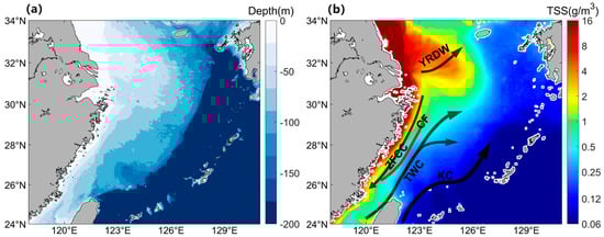
Figure 1.
(a) Topography and (b) schematic diagram of the circulation system in the East China Sea. In (b), the background color represents climatological TSS, and the red line indicates the Zhejiang–Fujian coastal turbidity front. KC: Kuroshio Current; TWC: Taiwan Warm Current; YRDW: Yangtze River Diluted Water; ZFCC: Zhejiang–Fujian Coastal Current. CF: Coastal Front.
The coastal water masses in the ECS are predominantly constituted by the Yangtze River Diluted Water (YRDW) and the Zhejiang−Fujian Coastal Water (ZFCW). The formation of these water masses is a consequence of the mixing of freshwater discharged from coastal rivers and shelf water, exhibiting characteristics such as turbidity, low salinity, and high nutrient concentrations [4]. The dispersal pathway of YRDW exhibits distinct seasonal variations: During summer months, a south−easterly deflection is exhibited, followed by a north−easterly turn [5] with its influence extending as far as Jeju Island or the central South Yellow Sea [6]. Conversely, during winter, the YRDW predominantly flows southward along the coast, eventually merging into the Zhejiang−Fujian Coastal Current [7,8]. Zhu [9] found that, under the influence of wind fields and upwelling, the diluted water of the Yangtze River can form a relatively isolated low−salinity mass in the northern East China Sea. Its separation and outward transport process significantly enhanced the cross-shelf transport efficiency of terrestrial nutrients and organic matter. The ZFCW is predominantly distributed in the western nearshore region of the ECS shelf. Its eastern boundary converges with the northward-flowing Taiwan Warm Current (TWC), forming a distinct Zhejiang–Fujian coastal front due to significant horizontal gradients in hydrographic properties. Conventional studies have suggested that the ZFCW and its associated pollutants, carbon particles, freshwater, and nutrients are unable to undergo large-scale cross-shelf offshore transport due to constraints imposed by frontal barriers and seabed topography. Instead, they were believed to be primarily transported southward to the Nan’ao Island area of Guangdong [10]. However, recent research has revealed the presence of large-scale frontal instability processes (penetrating fronts) in the Zhejiang–Fujian frontal zone. These processes have been shown to facilitate intermittent, large−scale cross-shelf offshore transport of nutrient-rich coastal waters, exerting significant influences on the physical-biogeochemical environment of the ECS shelf [11,12,13,14].
Yuan [11] was the first to identify large−scale, horizontally protruding cross−shelf penetrating fronts off the Yangtze Estuary and Zhejiang coast using MODIS SST and CHL imagery. He also confirmed the critical role of these fronts in cross−frontal and cross-shelf water exchange through in situ hydrographic and nutrient data analysis. He [13] analyzed 8−day composite MODIS and SeaWiFS SST/CHL data (1998–2007), revealing 2–11 annual occurrences of such penetrating fronts in this region. The frequency of these penetrating fronts was found to be notably higher during summer and winter months than in spring and autumn, with durations ranging from days to a month and maximum frontal lengths exceeding 300 km. In addition, Wu’s [15] examination of MODIS chlorophyll images during the autumn period (2003–2014) led to the identification of a recurrent autumn penetrating front situated along 28.5° N–29.5° N, characterized by a fixed positional pattern. Yin [16] employed GOCI satellite TSS imagery to quantitatively reconstruct the full evolution cycle (∼10 days) of Zhejiang coastal fronts—from submesoscale frontal waves to large-scale penetrating fronts—documenting three developmental phases: growth, maturation, and decay.
Current research on the offshore transport of coastal water masses in the ECS, particularly the ZFCW, remains insufficient and predominantly relies on case studies. There is a notable lack of systematic investigation into the transport locations and pathways. To address this gap, this study utilizes Total Suspended Sediments concentration (TSS) data from the Korean geostationary satellite GOCI (Geostationary Ocean Color Imager). The satellite has significant advantages in monitoring nearshore turbid water bodies. Compared with polar-orbiting satellites such as MODIS/VIIRS, GOCI can more effectively separate the radiation signals of turbid water bodies with its optimized band settings [14], effectively reducing the mean absolute error of suspended sediment concentration (SSC) inversion in high turbidity areas such as the Yangtze River Estuary. At the same time, GOCI’s high-frequency observation capability (once per hour, 8 scenes per day) and more than 80% effective data acquisition rate enable it to accurately capture the dynamic changes in tidally driven suspended sediment [17,18], while MODIS/VIIRS’s daily coverage rate is less than 30% [19]. Although Sentinel−3A/OLCI is superior to GOCI in the SSC inversion accuracy of Hangzhou Bay [20], its nearly 2−day observation period is difficult to meet the needs of short-term dynamic monitoring. In this paper, by employing positive TSS anomalies (∆TSS) after removing climatological means as a tracer for nearshore turbid water masses, we systematically analyze their spatiotemporal distribution through the spatial cumulative frequency of ∆TSS (). This approach aims to reveal the statistical patterns of offshore transport processes in ECS coastal waters.
2. Data and Methodology
2.1. GOCI-TSS
The East China Sea’s coastal water masses are characterized by low salinity, rich nutrients and high turbidity, so satellite−observed turbidity data can be used to track the horizontal transport of these water masses. This study utilizes TSS data observed by the GOCI as the tracer dataset. The GOCI has a spatial resolution of 500 m and a temporal resolution of 1 h, covering a time span from 08:16 to 15:45 Beijing Time. In comparison with polar−orbiting satellites, GOCI offers distinct advantages in its ability to monitor variations in ocean color information from a geostationary platform, facilitating the observation of short-term regional marine phenomena. This provides valuable data for studying the intermittent offshore transport processes of coastal waters. Ruddick [21] conducted a comparative analysis of GOCI and MODIS_AQUA’s Rrs and TSS products in the Bohai Sea region. The results indicated that the TSS distribution aligned with previous research findings. Although there is room for improvement in GOCI’s calibration, atmospheric correction, and inversion algorithms, the existing results demonstrate that GOCI’s data products can be effectively used to study dynamic processes in turbid waters. The TSS data from GOCI can be downloaded from the website of the Korea Ocean Satellite Center (https://kosc.kiost.ac.kr) accessed on 1 April 2024.
2.2. Sea Surface Wind
Sea surface winds have been demonstrated to influence the spatial distribution of TSS by driving vertical mixing and horizontal transport [22]. Therefore, this study employs the Cross−Calibrated Multi-Platform (CCMP) gridded sea surface wind data provided by the Remote Sensing System to investigate the impact of wind stress on TSS distribution. This dataset integrates buoy observations, satellite data (QuikSCAT and ASCAT), and ERA−Interim model outputs using a Variational Analysis Method, with a spatial resolution of 0.25° and a temporal resolution of 6 h. Comparative analyses between CCMP wind data and in situ observations show minimal discrepancies (approximately 0.5 m/s) [23], confirming that CCMP wind data provide reliable meteorological data for studying regional ocean dynamics. The dataset is available for download from the website: https://www.remss.com/measurements/ccmp/ accessed on 1 April 2024.
2.3. Tide Current
Tidal-induced mixing is a crucial dynamic process responsible for the resuspension of bottom sediments, significantly influencing the spatial distribution of TSS [24]. To minimize interference from TSS variations caused by tidal vertical mixing in this study, it is necessary to identify regions where tidal mixing is fully developed. This research employs tidal current data along the Zhejiang–Fujian coast, predicted by the global tidal model TPXO developed by Oregon State University, to calculate the Simpson–Hunter parameter for tidal mixing [25]. Based on thresholds established in previous studies, the boundaries of fully mixed tidal regions are delineated. The TPXO global tidal model is a widely used tidal simulation model developed by assimilating satellite altimetry data (e.g., TOPEX/Poseidon, Jason series) and tide gauge observations. It employs harmonic analysis and data assimilation techniques, optimizing tidal parameters via least-squares methods to enhance simulation accuracy. Recognized for its high precision and reliability, the TPXO model has been extensively applied in global tidal studies, demonstrating strong consistency with observations across various oceanic regions [26]. The model data can be downloaded from the website https://www.tpxo.net/global accessed on 1 April 2024.
2.4. Topographic Data
The bathymetric data used in this study were obtained from the latest global seabed and land elevation model, GEBCO_2023, released by the General Bathymetric Chart of the Oceans (GEBCO). This dataset integrates multi−source data, including shipborne multibeam bathymetry, remote sensing satellite observations, sub-ice topography estimations, and terrestrial elevation data [27,28], providing global elevation coverage at a 15-arc-second grid resolution in meters. Its accuracy has been validated, particularly in shallow waters, where comparisons with ICESat-2 satellite-derived seabed measurements demonstrate excellent performance of GEBCO_2023 [28]. As such, this dataset is widely applied in marine scientific research, ocean engineering, climate modeling, and ecological conservation, serving as a fundamental tool for analyzing oceanic and terrestrial topography [29].
2.5. Calculation of Residual Current Field
In order to analyze the influence of the ECS’s circulation system on the offshore transport pathways of coastal water masses, this study employed the Maximum Cross−Correlation (MCC) algorithm [30] to derive the surface current fields along the Zhejiang–Fujian coast from continuous TSS satellite imagery. The MCC method estimates the displacement of surface water features between sequential satellite images. It identifies the shift (in direction and distance) that produces the highest correlation between image pairs, effectively capturing the horizontal movement of water masses. This approach allows for the derivation of surface residual currents without direct velocity measurements. To validate the reliability of the retrieved current fields, the tidal components within them were verified using the ECS tidal current fields simulated by the FVCOM model, as presented by Xuan et al. [31]. The M2 tidal constituent in Xuan’s model data aligns well with cotidal charts obtained from satellite altimeter and coastal tide gauge observations, demonstrating high accuracy in simulating the tidal current fields of the ECS and confirming the model’s reliability. Figure 2 compares the M2 tidal ellipses extracted from the retrieved current fields with those from the model data. The results demonstrate a strong agreement across most of the study area, with the exception of shallow nearshore regions, thereby indicating the high credibility of the retrieved surface current fields. The validated current fields were then processed by subtracting the concurrent tidal currents predicted by TPXO, yielding the residual current fields.
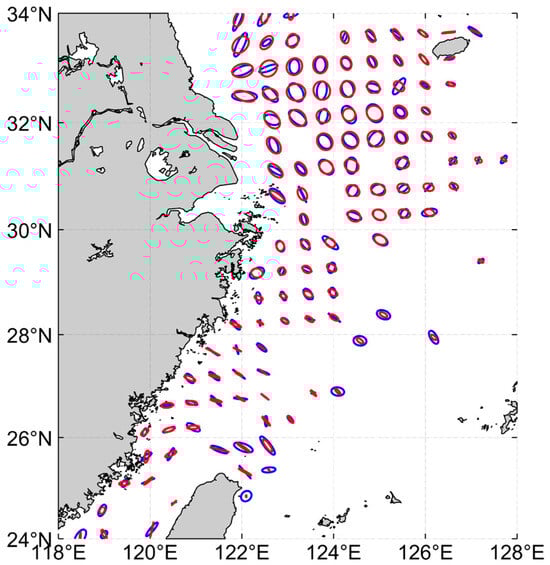
Figure 2.
Comparison of the M2 tidal current ellipse of the retrieved flow field (blue) and the model flow field (red).
2.6. Calculation of Spatial Cumulative Frequency of ΔTSS
In the East China Sea, water turbidity is typically high in coastal areas and low in offshore regions. When turbid coastal water masses are transported offshore, their TSS values are higher than the background TSS values of the surrounding areas. Therefore, positive TSS anomalies (ΔTSS) obtained by subtracting climatological means can serve as tracers for the offshore transport of coastal water masses. The principle behind using ΔTSS lies in anomaly detection. By subtracting the climatological monthly mean from hourly TSS values, we isolate short-term turbidity increases likely linked to offshore transport events. A pixel with ΔTSS > 0 suggests the presence of turbid coastal water moving into clearer offshore areas. By counting the frequency of such events (), we derive a statistical proxy for the intensity and recurrence of offshore transport over time. In order to statistically analyze the spatio-temporal distribution characteristics of the offshore transport pathways, the spatial cumulative frequency of ΔTSS () was calculated in this study using the following methodology:
Data pre-processing: To eliminate noise, TSS values greater than 100 g/m3 or equal to 0 g/m3 were set as NaN. The monthly climatological mean TSS () was then calculated.
Anomaly calculation: Hourly TSS satellite data were subtracted from the corresponding monthly climatological mean TSS to obtain hourly anomalies () (Figure 3b). If > 0, it indicates that the TSS value at that pixel and hour was higher than the background level, possibly due to offshore transport of highly turbid coastal waters (Figure 3a,b). In this study, sensitivity analysis was performed on the (Figure S1 of the support information), and the results showed that the selection of values did not affect the spatial distribution morphology of the transport path in the study area.
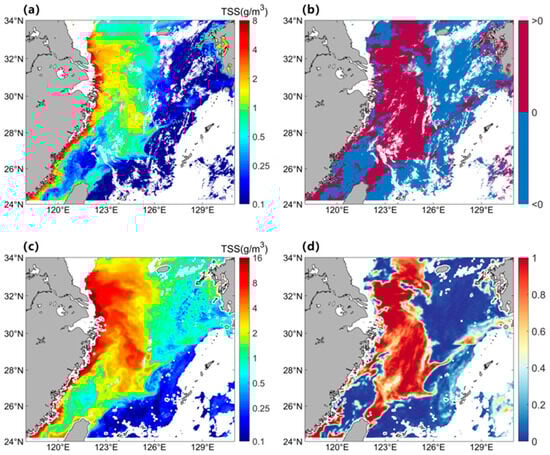
Figure 3.
Spatial distribution of (a) hourly TSS at 05:00, (b) at 05:00, (c) daily TSS, and (d) on 2 August 2015.
Cumulative frequency calculation: For each pixel, the number () of instances where is greater than 0 was divided by the total number () of cloud−free satellite images, yielding the spatial cumulative frequency of ΔTSS () (Figure 3d):
Using the above methodology, the climatological annual mean (), seasonal mean (), and monthly mean () spatial cumulative frequencies of ΔTSS were calculated.
2.7. Simpson–Hunter Tidal Mixing Index
Since this study focuses on the horizontal offshore transport processes of nearshore high−turbidity water masses, it is necessary to identify the extent of tidal mixing−dominated zones to avoid interference from tidal−induced TSS variations in the results. This study employs the Simpson–Hunter stratification parameter K [25] to determine the boundary of the fully tidally mixed zone, where , with H representing water depth and U denoting the characteristic tidal current velocity. This parameter has been widely used to locate tidal fronts (i.e., the boundaries of fully tidally mixed zones). Generally, when K > 3, the water column exhibits strong stratification, whereas when K < 1.5, it is fully mixed [16]. To delineate the maximum influence area of tidal vertical mixing, this study selects the maximum tidal current velocity as the characteristic tidal velocity. Following the approach of Zhao et al. [32] in their investigation of tidal mixing fronts in the Yellow Sea and northern ECS, a critical value of 1.8 is adopted to define the position of the tidal front.
3. Results and Discussion
3.1. Distribution Characteristics of Climatological TSS and Influencing Factors
3.1.1. Distribution Characteristics of Climatological TSS
The climatological monthly mean TSS data from May 2012 to December 2020 (Figure 4) reveal that the coastal waters of the East China Sea exhibit a typical spatial distribution pattern of high TSS concentrations nearshore and low concentrations offshore. Within the 20 m isobath, TSS concentrations are generally high and show an exponential decrease with increasing distance from the coast, nearly dropping to zero in shelf areas where water depth exceeds 80 m.
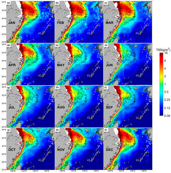
Figure 4.
(a–l) Climatological monthly mean TSS distribution from May 2012 to December 2020 (background color), with black contours indicating the 20 m, 50 m, and 80 m isobaths.
Additionally, TSS concentrations in the coastal East China Sea display pronounced seasonal variations. In the Subei Shoal and adjacent shelf areas north of the Yangtze River Estuary, TSS concentrations exhibit a “summer accumulation and winter transport” temporal pattern [33]. During summer, high TSS values are primarily confined within the 20 m isobath (Figure 4i), whereas in winter, high-TSS water masses expand southeastward to approximately the 80 m isobath on the shelf (Figure 4b). South of the Yangtze River Estuary along the Zhejiang–Fujian coastal waters, TSS concentrations generally follow a distribution pattern parallel to the coastline. High-turbidity coastal water masses are confined within the 50 m isobath, forming a distinct Zhejiang–Fujian coastal turbidity front at their boundary with low-turbidity shelf waters. In summer, the turbidity front is located closer to the shoreline, typically near the 20 m isobath (Figure 4i), while in winter, it extends outward to the vicinity of the 50 m isobath (Figure 4b).
3.1.2. Influencing Factors of TSS Climate State Distribution Characteristics
Previous studies have demonstrated that the distribution of surface TSS in the ECS is primarily influenced by tidal mixing, riverine input, wind-induced stirring, and circulation systems [33,34]. The coastal ECS is globally renowned as a strong tidal region, dominated by semidiurnal tides. The maximum tidal amplitude of the M2 constituent exceeds 1 m, with tidal current velocities reaching 1 m/s. Additionally, the S2 constituent exhibits a maximum amplitude of 0.6 m and a tidal current velocity of 0.5 m/s [35,36]. The vertical mixing caused by the strong interaction between tidal currents and coastal topography resuspends bottom sediments into surface waters, thereby dominating the spatial distribution of high TSS concentrations in coastal areas. In Figure 5, the contour of 1.8 (thick black line in Figure 5), representing the boundary of the tidally well−mixed zone [37], nearly coincides with the boundary of climatological high-TSS regions, further confirming the dominant role of tidal forcing in TSS distribution.
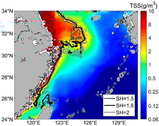
Figure 5.
Distribution of the Simpson–Hunter tidal mixing parameter K, with background colors representing the mean TSS from May 2012 to December 2020. Black contour lines denote K values of 1.5, 1.8, and 2, respectively.
Although the high-TSS distribution in the coastal East China Sea exhibits seasonal variations characterized by onshore contraction in summer and offshore expansion in winter [38,39], the underlying driving factors differ between the northern and southern sides of the Yangtze estuary.
North of the estuary on the Subei Shoal, TSS seasonality is primarily governed by vertical mixing intensity [40] and cross−shelf transport driven by the Yellow Sea Coastal Current (YSCC) [41,42]. During summer, southerly monsoon winds weaken the YSCC [14], thereby preventing the northward deflection of turbid coastal waters from reaching the shelf area between the 20–50 m isobaths. Furthermore, enhanced thermal stratification has been shown to reduce vertical mixing [37,43], thereby limiting sediment resuspension and confining high-TSS waters to the shoreward side of the 20 m isobath. Conversely, during winter, the northerly monsoons intensify the southward−flowing YSCC (Figure 6). When this current deflects northward near the Yangtze estuary, it transports substantial turbid coastal water masses onto the shelf [44]. Vigorous wind stirring and surface cooling induce full-depth mixing within the 50 m isobath, entraining bottom sediments into the surface layers [42,45]. This process drives the offshore expansion of high-TSS waters across the shelf region within the 50 m isobath [46].
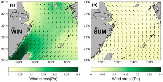
Figure 6.
Climatological winter (a) and summer (b) sea surface wind fields from May 2012 to December 2020. The background color represents wind stress, with arrows indicating wind vectors.
South of the Yangtze River estuary along the Zhejiang–Fujian coast, the seasonal variability of TSS is primarily controlled by the intensity variations in the Zhejiang–Fujian Coastal Current (ZFCC) and the TWC. During summer, the northeastward deflection of YRDW and the weakened southward ZFCC under southerly monsoons [47], coupled with the significantly strengthened northward TWC [48], shift the Zhejiang–Fujian coastal turbidity front closer to shore, typically positioned near the 20 m isobath [49,50,51]. In winter, the opposite pattern emerges: the YRDW extends southward alongshore and merges with the ZFCC, while northerly monsoons intensify the coastal current [52]. Concurrently, the TWC experiences a weakening under the influence of monsoon forcing [53]. Consequently, the turbidity front migrates offshore, typically located near the 50 m isobath.
3.2. Spatiotemporal Distribution of the
The climatological distribution of TSS (Figure 4 and Figure 5) demonstrates that coastal water masses in the ECS are primarily confined to nearshore areas within the 50 m isobath throughout the year. However, the image of hourly TSS (Figure 3) reveals intermittent offshore transport processes in this region. These processes have the capacity to transport high-turbidity coastal water masses extensively to the shelf area. Given the higher turbidity of coastal water masses compared to shelf water masses, the offshore transport of coastal water can be tracked by analyzing positive TSS anomalies (∆TSS). Furthermore, through spatiotemporal analysis of the spatial cumulative frequency of ∆TSS , we can elucidate the distribution patterns of offshore transport pathways for coastal water masses in the ECS.
3.2.1. The Climatological Spatial Distribution Characteristics of
As demonstrated in Figure 7, the climatological mean of the spatial cumulative frequency is predominantly minimal within the 20 m isobath. Between the 20 and 50 m isobaths, a band of high values extends from north to south, while beyond the 50 m isobath on the continental shelf, high−value zones are mainly distributed north of 28° N, extending as far as the edge of the ECS shelf. Conversely, a low-value zone is evident south of 28° N, extending northwestward from the shelf break northeast of Taiwan to the area between the 50 and 80 m isobaths. Furthermore, regions influenced by the Kuroshio Current, particularly along the shelf break of the ECS, generally exhibit low values. This suggests that long−distance cross-shelf offshore transport of high-turbidity coastal water masses primarily occurs in the northern ECS, reaching as far as the shelf edge, while cross-shelf transport in the southern ECS is largely constrained by the 50 m isobath. This phenomenon is further corroborated by the climatological surface chlorophyll concentration distribution in the ECS (Figure 7b). In the southeastern region, high chlorophyll concentrations are mainly confined to nearshore areas, whereas in the northern ECS, high chlorophyll zones extend from the coast to the shelf region.
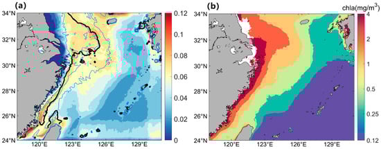
Figure 7.
(a) Climatological distribution of (May 2012–December 2020); (b) climatological distribution of Chl-a (June 2002–March 2024). In (a), the black contours indicating the K = 1.8 isoline and blue contours showing the 20 m, 50 m, and 80 m isobaths.
3.2.2. Seasonal Variability of Distribution
From Figure 8, it can be seen that the distribution of exhibits not only significant spatial differences but also pronounced seasonal variations, characterized by higher values in summer and lower values in winter. In winter, remains generally low, both in nearshore areas within the 50 m isobath and in the shelf region beyond it (Figure 8a). In spring, remains low south of 29° N, while it increases significantly to 0.08 in Hangzhou Bay and the outer Yangtze River estuary north of 29° N, with the high-value zone extending as far as approximately 127.5° E (Figure 8b). During summer, is about 0.12−0.14, reaching its annual peak in the ECS, forming a high−value belt between the 20 m and 80 m isobaths from north to south. Around 30° N, the high-value zone extends beyond the 80 m isobath, reaching as far as approximately 129° E in the Kuroshio region (Figure 8c). In autumn, the spatial distribution of is similar to that in summer, but its overall values significantly decrease to 0.06–0.1. The high-value belt north of Hangzhou Bay contracts within the 80 m isobath, while the high-value belt south of Hangzhou Bay retreats within the 50 m isobath (Figure 8d). Although this study mainly focuses on the offshore transport pathways and physical mechanisms of nearshore highly turbid waters, these processes may also trigger important responses at the ecosystem level. Taking summer as an example, there are the most transport channels and the widest coverage, indicating that a large amount of nearshore water masses containing nutrients may be transported to the shelf area. After these nitrogen− and phosphorus−rich waters enter the relatively clear surface of the shelf, they may induce local or regional phytoplankton algal bloom events [54], thereby changing the pattern of primary productivity [55]. In addition, the characteristics of particulate organic carbon (POC) attached to suspended sand also make these transport pathways potential carbon export pathways [56], which help promote the cross−shelf carbon flux process and affect the regional carbon cycle. However, excessive suspended matter transported to the open sea will block sunlight, inhibit photosynthesis, and affect primary production [57,58].
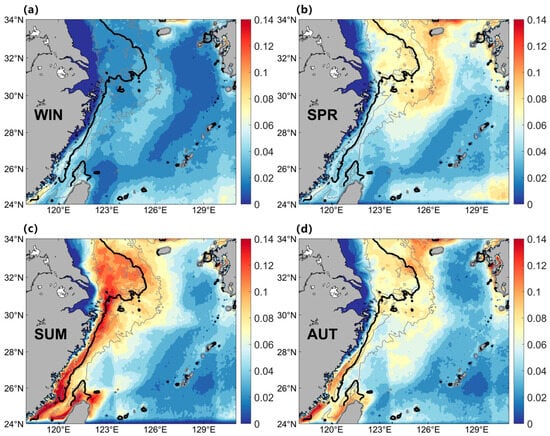
Figure 8.
Seasonal distribution of the climatological from May 2012 to December 2020. (a) Winter. (b) Spring. (c) Summer. (d) Autumn. The black contours indicate the K = 1.8 isoline and gray contours show the 20 m, 50 m, and 80 m isobaths.
3.3. Spatial-Temporal Distribution of Offshore Transport Pathways of Coastal Water Masses
As shown in Figure 7 and Figure 8, the spatial cumulative frequency of suspended sediment concentration anomalies (∆TSS), denoted as , exhibits pronounced spatial heterogeneity and seasonal variability. This reflects the highly dynamic nature of offshore transport processes of coastal turbid water masses. To comprehensively examine the spatiotemporal distribution of these offshore transport pathways, this study integrates the monthly mean spatial distribution of with satellite-derived sea surface residual current fields (Figure 9). To isolate the influence of horizontal transport, the analysis focuses on regions outside the tidally well−mixed zone, delineated by the Simpson–Hunter parameter K = 1.8 (black line in Figure 9). Persistent high-value zones were observed beyond this boundary, indicating frequent offshore movement of coastal high-turbidity waters. Source-tracking analysis was conducted on these high-value zones to identify the origin and pathways of offshore transport, as indicated by the purple arrows in Figure 9.
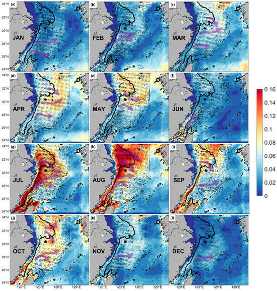
Figure 9.
(a–l) Climatological monthly mean distribution of from May 2012 to December 2020. Black arrows represent the residual current field derived from satellite observations, the black line denotes the K = 1.8 tidal mixing parameter contour, and semi-transparent purple arrows indicate potential offshore transport pathways.
Between January and June, values across the East China Sea (ECS) remained generally below 0.1. In January and February, one to two offshore transport pathways were identified along the Zhejiang and Fujian coasts between 26° N and 30° N, extending either southeastward or northeastward. In March, increased significantly in the northern ECS, from 0.02 to 0.08, particularly near the Yangtze River estuary and Subei Shoal, with three offshore pathways emerging. These patterns largely persisted through April, although the high-value zone of about 0.1 near 28° N disappeared in May, and the number of pathways decreased to two. In June, offshore transport activity reached its minimum, with only a single alongshore pathway forming near the tidally mixed region of the Taiwan Strait. Transport activity intensified in July and August, with exceeding 0.12 and reaching 0.16 in some areas, reaching its annual peak in the northern part of the ECS. The High−value zones exceeding 0.12 extended to the continental shelf edge, and the number of offshore transport pathways increased to three or four. These originated from the Yangtze River estuary, Subei Shoal, and near 28° N, extending southeastward or northeastward. In September, the number of pathways decreased to two as transport activity declined. In November and December, offshore transport pathways were largely absent, with only a persistent eastward pathway observed near 28° N.
The offshore transport pathways of the Zhejiang–Fujian coastal waters exhibit clear spatiotemporal heterogeneity, with the frequency and number of transport events peaking in summer (up to four pathways) and dropping to a minimum in winter (one pathway). Except for January, all identified pathways are located north of 28° N. Among these, the pathway near 28° N is the most persistent, present in all months except May and June. Its formation is closely linked to the dynamics of the Taiwan Warm Current (TWC). Originating from coastal waters south of 28° N, this pathway is driven northeastward by the northward flow of the TWC, then turns eastward under the influence of its bifurcation, eventually reaching the ECS shelf edge. An additional pathway between 29° N and 30° N occurs during February–May and August, extending eastward and reaching waters near 126° E. This aligns well with the position of the penetrating front described by Wu [15], which is typically observed under prevailing northerly monsoon conditions and is attributed to thermocline oscillations driven by spatially uneven tidal mixing. Moreover, a southeastward transport pathway off the north bank of the Yangtze estuary appears in most months except January–February, June, and November–December. This finding deviates from the traditional “summer accumulation, winter transport” paradigm of Subei Shoal sediment dynamics. Instead, it suggests a summer−dominant transport mechanism possibly linked to the seasonal extension of the Yangtze River Diluted Water (YRDW). This interpretation is supported by Lie and Cho [59], who reported that the YRDW flows northeastward then southeastward in summer after exiting the estuary, consistent with the pathway identified in this study.
4. Conclusions
The offshore transport process of coastal water masses in the East China Sea (ECS) plays a crucial role in supporting the regional marine ecosystem. This study employs TSS concentration data from the Korean GOCI satellite. By analyzing the climatological distribution of TSS and the spatial cumulative frequency of positive TSS anomalies (), in conjunction with satellite−derived surface residual currents, we systematically investigate the spatio-temporal characteristics of offshore transport for coastal water masses in the ECS. The main findings are summarized as follows:
- Dominant spatial pattern of nearshore turbidity waters
Nearshore waters in the ECS consistently exhibit a “high nearshore, low offshore” TSS distribution pattern. High-turbidity water masses are mainly confined within the 20–50 m isobath range, with a clear seasonal shift—extending southeastward to the 50 m isobath in winter and retreating shoreward to the 20 m isobath in summer.
- 2.
- Spatio-temporal heterogeneity of offshore transport patterns
The offshore transport of high-turbidity water masses shows pronounced spatial and seasonal variability.
Seasonally, summer (June–August) is the peak transport period, featuring up to four active pathways and the broadest spatial coverage. In contrast, winter (December–February) is marked by only one main pathway and reduced transport frequency, while spring and autumn display transitional characteristics.
Spatially, pathways north of 28° N can extend to the shelf edge (~129° E), indicating relatively unobstructed offshore movement. South of 28° N, however, the northward branch of the Taiwan Warm Current (TWC) acts as a physical barrier, confining transport within the 50 m isobath.
- 3.
- Identification of persistent and seasonal transport pathways
A persistent transport pathway near 28° N is observed year-round (except during May–June), likely driven by the eastward branch of the TWC. This pathway extends northeastward to ~126° E, then turns eastward toward the shelf edge (~129° E).
Two additional seasonal pathways are identified:
- One located south of Hangzhou Bay (~30° N), active during February–May and August, is likely linked to tidal-induced thermocline oscillations. Its location aligns with the penetrating front reported by Wu [15].
- Another located off the north bank of the Yangtze River Estuary appears exclusively in summer and follows a southeastward trajectory consistent with the expansion of the Yangtze River Diluted Water (YRDW). This challenges the conventional “summer accumulation, winter transport” paradigm and highlights the significance of summer offshore export processes in the northern ECS.
These findings provide new observational insights into the offshore transport dynamics of coastal water masses in the ECS. They enhance our understanding of the spatial structure and seasonal variability of transport pathways and carry important implications for material exchange, nutrient cycling, and the ecological stability of the continental shelf system. Future research should integrate numerical modeling with field observations to better quantify the roles of various physical drivers and to improve the predictive capability of material transport processes under evolving environmental conditions.
Supplementary Materials
The following supporting information can be downloaded at: https://www.mdpi.com/article/10.3390/w17091370/s1, Figure S1: Sensitivity test diagram of ∆TSS, the figure represents on 2 August 2015. (a) takes ∆TSS > 0, (b) takes ∆TSS > 0.05, (c) takes ∆TSS > 0.1.
Author Contributions
Methodology, W.Y.; software, Y.P.; validation, Y.P.; formal analysis, W.Y.; data curation, Y.P., writing—original draft preparation, Y.P. and W.Y.; review and editing, W.Y., visualization, Y.P.; supervision, W.Y.; funding acquisition, W.Y. All authors have read and agreed to the published version of the manuscript.
Funding
Yuanjie Peng and WenBin Yin was funded by the Science and Technology Project of Zhoushan (Grant No. 2023C41020) and the National Natural Science Foundation of China (Grant No. 41906025).
Data Availability Statement
The TSS data from GOCI can be downloaded from the website of the Korea Ocean Satellite Center (https://kosc.kiost.ac.kr) (accessed on 1 April 2025) The CCMP dataset is available to download from the website http://www.remss.com/measurements/ccmp/ (accessed on 1 April 2025). The TPXO model data can be downloaded from the website https://www.tpxo.net/global (accessed on 2 April 2025). The FVCOM model data were obtained from Xuan [31] in 2016. The data can be downloaded from the website https://figshare.com/account/home (accessed on 20 April 2025).
Conflicts of Interest
The authors declare no conflicts of interest.
References
- Liu, S.; Han, S.; Wei, Y. Analysis of water mass in the northwest of the East China Sea and its relationship with fishing grounds. J. Fish. China 1984, 8, 125–133. [Google Scholar]
- Wu, L.; Wei, Q.; Xin, M. Spatial distribution patterns of nutrients and controlling mechanisms in the East China Sea during spring. Adv. Mar. Sci. 2023, 41, 622–636. [Google Scholar]
- Liu, D.; Qiao, L.; Li, G. Suspended matter transport, flux and seasonal variation in the inner shelf of the East China Sea. Oceanol. Et Limnol. Sinica 2022, 49, 24–39. [Google Scholar]
- Guan, B. Patterns and Structures of the Currents in Bohai, Huanghai and East China Seas. In Institute of Oceanology; Springer: Berlin/Heidelberg, Germany, 1994. [Google Scholar]
- Guo, Y.; Rong, Z.; Chi, Y.; Li, X.; Na, R. Numerical Study on the Interannual Variation of the Changjiang Diluted Water in Summer. Ocean. Limnol. Bull. 2020, 4, 30–41. [Google Scholar]
- Mao, H.; Gan, Z.; Lan, S. Preliminary study on the Changjiang diluted water and its mixing. J. Oceanol. Limnol. 1963, 5, 183–206. [Google Scholar]
- Beardsley, R.; Limeburner, R.; Yu, H.; Cannon, G. Discharge of the Changjiang (Yangtze River) into the East China sea. Cont. Shelf Res. 1985, 4, 57–76. [Google Scholar] [CrossRef]
- Yuan, Y.; Su, J.; Zhao, J. A single-layer model of continental shelf circulation in the East China Sea. Acta Oceanol. Sin. 1982, 4, 1–11. [Google Scholar]
- Zhu, B.; Yang, W.; Jiang, C.; Wang, T.; Wei, H. Observations of turbulent mixing and vertical diffusive salt flux in the Changjiang Diluted Water. J. Oceanol. Limnol. 2022, 40, 1349–1360. [Google Scholar] [CrossRef]
- Wang, C.; Guo, X.; Fang, J.; Li, Q. Seasonal characteristics of the extension range of Fujian-Zhejiang Coastal Current and its influence on typical bays. J. Appl. Oceanogr. 2018, 37, 1–8. [Google Scholar]
- Yuan, D.; Qiao, F.; Su, J. Cross-shelf penetrating fronts off the southeast coast of China observed by MODIS. Geophys. Res. Lett. 2005, 32, L19603. [Google Scholar] [CrossRef]
- Yuan, D.; Li, Y.; He, L.; Zhou, H.; Li, R.; Wang, F.; Lei, H.; Hu, D. An observation of the three-dimensional structure of a cross-shelf penetrating front off the Changjiang mouth. Deep. Sea Res. Part II Top. Stud. Oceanogr. 2010, 57, 1827–1834. [Google Scholar] [CrossRef]
- He, L.; Li, Y.; Zhou, H.; Yuan, D. Variability of cross-shelf penetrating fronts in the East China Sea. Deep. Sea Res. Part II Top. Stud. Oceanogr. 2010, 57, 1820–1826. [Google Scholar] [CrossRef]
- Li, Y. Summertime Circulation Characteristics and Its Dynamic Mechanism in the Coastal Waters of Eastern China. Ph.D. Thesis, Institute of Oceanography, Chinese Academy of Sciences, Qingdao, China, 2010. [Google Scholar]
- Wu, H. Cross-shelf penetrating fronts: A response of buoyant coastal water to ambient pycnocline undulation. J. Geophys. Res. Ocean. 2015, 120, 5101–5119. [Google Scholar] [CrossRef]
- Yin, W.; Huang, D. Evolution of submesoscale coastal frontal waves in the East China Sea based on geostationary ocean color imager observational data. Geophys. Res. Lett. 2016, 43, 9801–9809. [Google Scholar] [CrossRef]
- Peng, X.; Shen, F. Comparative Analysis of Suspended Particulate Matter Concentration in Yangtze Estuary Derived by Several Satellite Sensors. Infrared 2014, 35, 31. [Google Scholar]
- Yeom, J.-M.; Kim, H.-O. Comparison of NDVIs from GOCI and MODIS data towards improved assessment of crop temporal dynamics in the case of paddy rice. Remote Sens. 2015, 7, 11326–11343. [Google Scholar] [CrossRef]
- Liu, X.; Yang, Q.; Liu, Q. Adaptability analysis of various versions of GDPS in GOCI data processing in the Yellow Sea based on QA Score. Spectrosc. Spectr. Anal. 2021, 41, 2233–2239. [Google Scholar]
- Yu, Z.; Wang, J.; Li, Y. Remote sensing of suspended sediment in high turbid estuary from sentinel-3A/OLCI: A case study of Hangzhou Bay. Front. Mar. Sci. 2022, 9, 1008070. [Google Scholar] [CrossRef]
- Ruddick, K.; Vanhellemont, Q.; Yan, J.; Neukermans, G.; Wei, G.; Shang, S. Variability of suspended particulate matter in the Bohai Sea from the geostationary Ocean Color Imager (GOCI). Ocean. Sci. J. 2012, 47, 331–345. [Google Scholar] [CrossRef]
- Yang, Z.; Lei, K.; Guo, Z.; Wang, H. Effect of a winter storm on sediment transport and resuspension in the distal mud area, the East China Sea. J. Coast. Res. 2007, 23, 310–318. [Google Scholar] [CrossRef]
- Zheng, C. Based on CCMP wind field, the characteristics of sea surface wind field in China seas in the past 22 years are analyzed. Res. Meteorol. Disaster Reduct. 2011, 34, 41–46. [Google Scholar]
- Zhang, W.; Zhu, S.; Li, X.; Ruan, K.; Guan, W.; Peng, J. The effects of tidal residual current and tidal mixing on the low-salinitywater mass in the northeastern sea area outside the Yangtze Estuary. Acta Oceanol. Sinica 2014, 36, 9–18. [Google Scholar]
- Simpson, J.H.; Hunter, J. Fronts in the Irish sea. Nature 1974, 250, 404–406. [Google Scholar] [CrossRef]
- Tian, Z.; Wang, C.; Yu, Z.; Liu, H.; Lin, P.; Li, Z. Tide simulation in a global eddy-resolving ocean model. Acta Oceanol. Sin. 2024, 43, 1–10. [Google Scholar] [CrossRef]
- Morlighem, M. Measures Bedmachine Antarctica, Version 2; National Snow and Ice Data Center: Boulder, CO, USA, 2020. [Google Scholar]
- Giribabu, D.; Hari, R.; Sharma, J.; Ghosh, K.; Padiyar, N.; Sharma, A.; Bera, A.K.; Srivastav, S.K. Performance assessment of GEBCO_2023 gridded bathymetric data in selected shallow waters of Indian ocean using the seafloor from ICESat-2 photons. Mar. Geophys. Res. 2024, 45, 1. [Google Scholar] [CrossRef]
- Smith, W.H.; Sandwell, D.T. Global sea floor topography from satellite altimetry and ship depth soundings. Science 1997, 277, 1956–1962. [Google Scholar] [CrossRef]
- Ma, Y.; Yin, W.; Guo, Z.; Xuan, J. The ocean surface current in the East China Sea computed by the Geostationary Ocean Color Imager satellite. Remote Sens. 2023, 15, 2210. [Google Scholar] [CrossRef]
- Xuan, J.; Huang, D.; Pohlmann, T.; Su, J.; Mayer, B.; Ding, R.; Zhou, F. Synoptic fluctuation of the Taiwan Warm Current in winter on the East China Sea shelf. Ocean. Sci. 2017, 13, 105–122. [Google Scholar] [CrossRef]
- Zhao, B. Distribution of tidal shelf fronts in the Yellow Sea. Bohai Seas 1987, 5, 16–23. [Google Scholar]
- Qiao, L. Suspended Sediment Transport, Flux, and Seasonal Variation on the East China Sea Inner Shelf. Ocean. Lakes 2018, 49, 16. [Google Scholar]
- Zhou, Y.; Xuan, J.; Huang, D. Tidal variation of total suspended solids over the Yangtze Bank based on the geostationary ocean color imager. Sci. China Earth Sci. 2020, 63, 1381–1389. [Google Scholar] [CrossRef]
- Zhao, B.; Fang, G.; Cao, D. Numerical simulation of tidal current in Bohai Sea, Yellow Sea and East China Sea. J. Oceanogr. (Chin. Version) 1994, 16, 10. [Google Scholar]
- Lin, Z.; Zhu, X.; Bao, X.; Liu, Q. Numerical simulation of three-dimensional tide and tidal current in Quanzhou Bay based on FVCOM. J. Oceanogr. (Chin. Version) 2013, 35, 15–24. [Google Scholar]
- Zhao, B. Yellow Sea Cold Water Mass front mixed with tide. Ocean. Lakes 1985, 16, 451–460. [Google Scholar]
- Chang, P.H.; Isobe, A. A numerical study on the Changjiang diluted water in the Yellow and East China Seas. J. Geophys. Res. Ocean. 2003, 108, 3299. [Google Scholar] [CrossRef]
- Chang, Y.; Lee, M.; Shimada, T.; Sakaida, F.; Kawamura, H.; Chan, J.; Lu, H. Wintertime high-resolution features of sea surface temperature and chlorophyll—A fields associated with oceanic fronts in the southern East China Sea. Int. J. Remote Sens. 2008, 29, 6249–6261. [Google Scholar] [CrossRef]
- Cheng, X.; Sun, Q.; Wang, Y.; Yang, Y. Seasonal Variation and Structural Analysis of the Tidal Front Outside the Jiangsu Bank Radial Sand Ridges. Mar. Sci. 2017, 41, 1–8. [Google Scholar]
- Guo, Z.; Yang, Z.; Zhang, D.; Fan, D.; Lei, K. Winter, summer distribution of suspended matter in the northern East China Sea and the blocking effect of ocean currents on suspended matter transport. J. Oceanogr. 2002, 24, 71–80. [Google Scholar]
- Yang, Z.; Guo, Z.; Wang, Z.; Xu, J.; Gao, W. The macroscopic pattern of the transport of suspended matter from the continental shelf of the Yellow Sea and East China Sea to its eastern deep sea area. Acta Oceanol. Sin. 1992, 14, 81–90. [Google Scholar]
- Tang, Y.; Zou, E.; Li, X.; Li, Z. Some characteristics of the circulation in the South Yellow Sea. Acta Oceanol. Sin. 2000, 22, 1–16. [Google Scholar]
- Bian, C. Sediment Transport in the Nearshore Area of China in the Bohai Sea, Yellow Sea and East China Sea. Ph.D. Dissertation, Ocean University of China, Qingdao, China, 2012. [Google Scholar]
- Bao, X.; Li, Z.; Wang, Y.; Li, N. Winter and Summer Distribution Characteristics of Suspended Matter in the Northern Yellow Sea. Sediment Res. 2010, 2, 48–56. [Google Scholar]
- Chen, Y. Numerical Simulation of Seasonal Continuous Variation of the Yellow Sea-East China Sea Circulation and the Changjiang Diluted Water. Master′s Thesis, East China Normal University, Shanghai, China, 2007. [Google Scholar]
- Qi, J. Characteristics of the East Sea Water Mass and a Study of the Kuroshio Current’s Exchange with East China Sea Shelf Water. Ph.D. Thesis, School of the Chinese Academy of Sciences (Institute of Oceanology), Qingdao, China, 2014. [Google Scholar]
- Lin, X.; Hou, L.; Liu, M.; Li, X.; Yin, G.; Zheng, Y.; Deng, F. Gross nitrogen mineralization in surface sediments of the Yangtze Estuary. PLoS ONE 2016, 11, e0151930. [Google Scholar] [CrossRef] [PubMed]
- Shi, X.; Li, H.; Wang, H.; Wang, L.; Zhang, C. Preliminary Study on the Hydrochemical Characteristics of the Taiwan Warm Current in Summer and Its Impact on the Frequent Occurrence Area of Red Tide in the East China Sea. Ocean. Lakes 2013, 44, 1208–1215. [Google Scholar]
- Luo, Y.; Yu, G. Numerical calculation of upwelling along the East China Sea caused by wind and Taiwan warm current. J. Qingdao Ocean. Univ. (Nat. Sci. Ed.) 1998, 28, 536–542. [Google Scholar]
- Bao, M.; Guan, W.; Cao, Z.; Chen, Q.; Yang, Y. Marine Ecological Disasters and Their Physical Controlling Mechanisms in Jiangsu Coastal Area. In Coastal Environment, Disaster, and Infrastructure—A Case Study of China’s Coastline; IntechOpen: London, UK, 2018. [Google Scholar]
- Wang, J.; Si, G.; Yu, F. Research Progress on Variation Characteristics and Mechanism of Taiwan Warm Current. Mar. Sci. 2020, 44, 141–148. [Google Scholar]
- Sun, X.; Fang, M.; Huang, W. The temporal and spatial variation of suspended matter transport in the Yellow Sea and East China Sea continental shelf area. Ocean. Lakes 2000, 6, 581–587. [Google Scholar]
- Yuan, Y. Study on the Distribution and Key Processes of Nutrients in Typical Sea Areas Under Different Backgrounds of Human Activities and Natural Driving. Ph.D. Thesis, School of the Chinese Academy of Sciences (Institute of Oceanology), Qingdao, China, 2016. [Google Scholar]
- Liu, K.; Chao, S.; Lee, H.; Gong, G.; Teng, Y. Seasonal variation of primary productivity in the East China Sea: A numerical study based on coupled physical-biogeochemical model. Deep. Sea Res. Part II Top. Stud. Oceanogr. 2010, 57, 1762–1782. [Google Scholar] [CrossRef]
- Zhao, B.; Yao, P.; Bianchi, T.; Yu, Z. Controls on organic carbon burial in the Eastern China marginal seas: A regional synthesis. Glob. Biogeochem. Cycles 2021, 35, e2020GB006608. [Google Scholar] [CrossRef]
- Wang, Y.; Wu, H.; Lin, J.; Zhu, J.; Zhang, W.; Li, C. Phytoplankton blooms off a high turbidity estuary: A case study in the Changjiang River Estuary. J. Geophys. Res. Ocean. 2019, 124, 8036–8059. [Google Scholar] [CrossRef]
- Llames, M.E.; Lagomarsino, L.; Diovisalvi, N.; Fermani, P.; Torremorell, A.M.; Pérez, G. The effects of light availability in shallow, turbid waters: A mesocosm study. J. Plankton Res. 2009, 31, 1517–1529. [Google Scholar] [CrossRef]
- Lie, H.J.; Cho, C.H.; Lee, J.H.; Lee, S. Structure and eastward extension of the Changjiang River plume in the East China Sea. J. Geophys. Res. Ocean. 2003, 108, 3077. [Google Scholar] [CrossRef]
Disclaimer/Publisher’s Note: The statements, opinions and data contained in all publications are solely those of the individual author(s) and contributor(s) and not of MDPI and/or the editor(s). MDPI and/or the editor(s) disclaim responsibility for any injury to people or property resulting from any ideas, methods, instructions or products referred to in the content. |
© 2025 by the authors. Licensee MDPI, Basel, Switzerland. This article is an open access article distributed under the terms and conditions of the Creative Commons Attribution (CC BY) license (https://creativecommons.org/licenses/by/4.0/).