
Resilience Assessment Method of Urban Flooding Prevention and Control System (FPC) Based on Attribute Resilience (AR) and Functional Resilience (FR)


Abstract
1. Introduction
2. Methodology
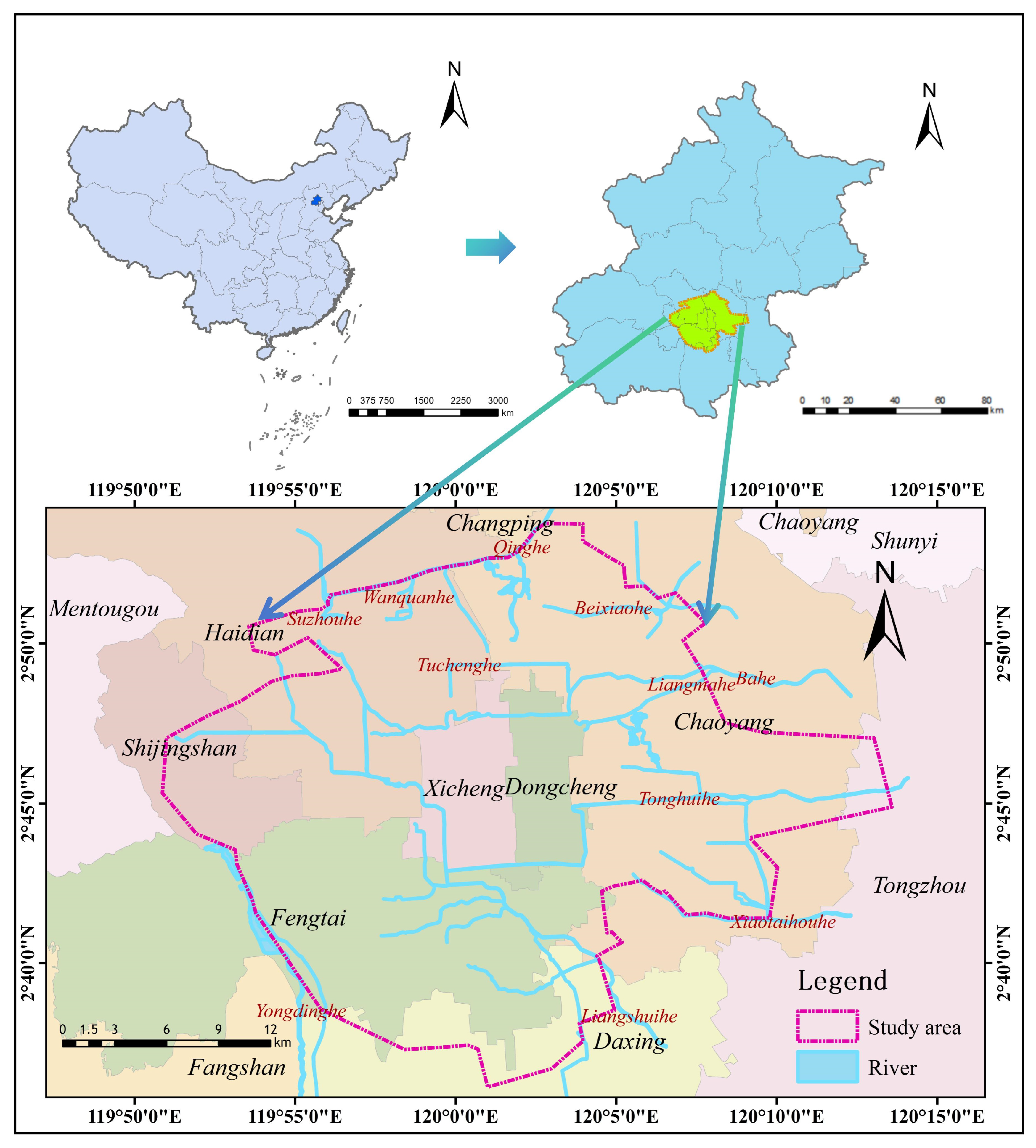
2.1. Study Area
2.2. Resilience Assessment Framework of FPC
2.3. Evaluation System of AR
2.3.1. Construction of Evaluation Index System for AR
2.3.2. Calculation Method of AR Based on EWM-TOPSIS
2.4. Evaluation Method of FR for FPC
2.4.1. Construction of Urban Flood Hydrodynamic Model
2.4.2. Calculation Method of FR
2.5. AR and FR Spatial Autocorrelation Analysis
2.5.1. Univariate Spatial Autocorrelation
2.5.2. Bivariate Spatial Autocorrelation
3. Result
3.1. Evaluation Results of AR of Urban FPC Based on EWM-TOPSIS
3.1.1. Weight of Resilience Evaluation Indicators
3.1.2. Evaluation Results of AR
3.2. FR Based on Hydrodynamic Model
3.2.1. Result of Flood Risk
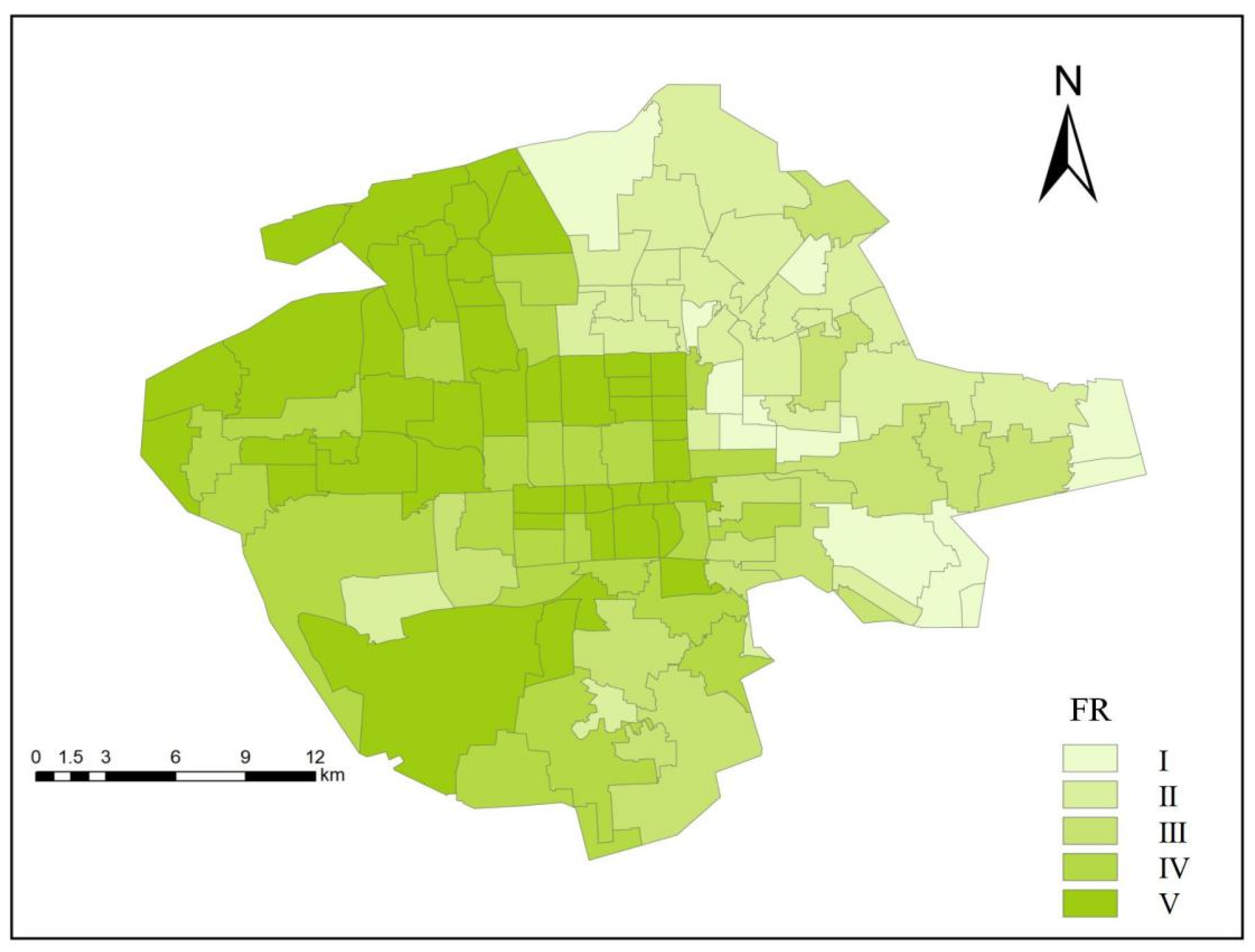
3.2.2. Spatial Distribution of FR
3.3. Spatial Correlation Analysis of Flood Resilience
3.3.1. Univariate Spatial Autocorrelation Analysis of Resilience
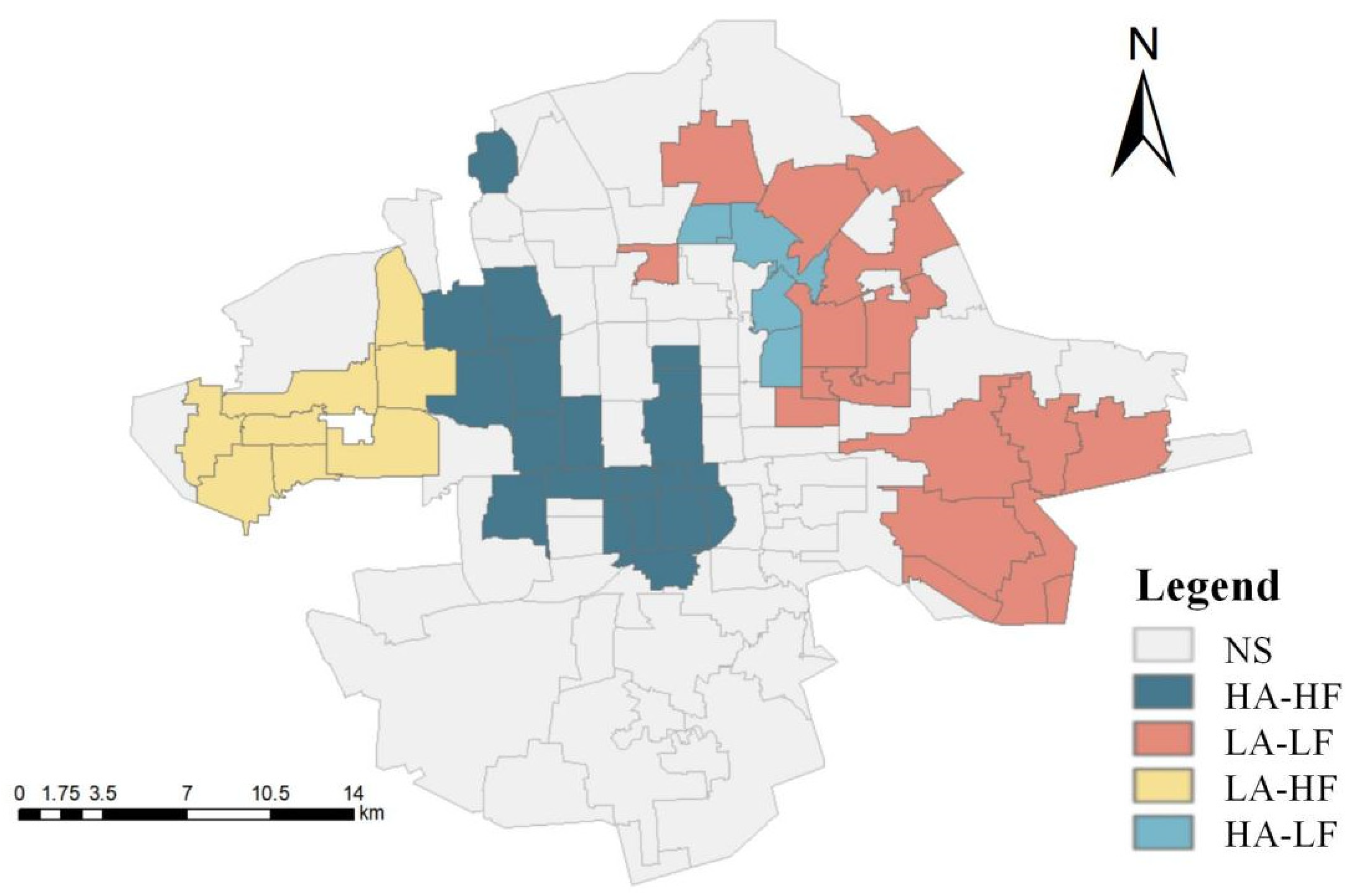
3.3.2. Bivariate Spatial Autocorrelation Analysis of AR and FR
4. Discussion
5. Conclusions
- (1)
- The AR analysis identifies key factors influencing the FPC. Using the EWM, this study determined that the GSP, average slope, and DC are the critical factors affecting AR. In areas with a low GSP, small slope, and insufficient DC, the AR is generally low due to high runoff and limited drainage capacity. Further analysis shows that among the three dimensions of AR (resistance, absorption, and recovery), absorption has the most significant impact, with a weight of 0.447. This indicates that drainage and storage facilities play a crucial role in enhancing the AR. Future strategies for improving flood resilience should prioritize GSP development, slope optimization, and the enhancement of drainage capacity while focusing on improving absorption and recovery to achieve a more balanced resilience distribution.
- (2)
- This study evaluated urban AR and FR, revealing that the AR has an uneven spatial distribution and generally low levels. Sub-districts with high resistance are mainly located in peripheral regions, high recovery areas are concentrated in central regions, and sub-districts with high absorption are rare. In contrast, the FR exhibits higher levels overall, with resilience-weak areas predominantly distributed in the northeastern region. Future efforts should target these resilience-weak areas, optimizing spatial layouts and improving the coordination of resistance, absorption, and recovery to enhance overall urban flood resilience
- (3)
- The Moran’s I indices for the AR and FR were calculated as 0.66 and 0.49, respectively, indicating significant spatial clustering, though the clustering locations differ. The spatial autocorrelation analysis demonstrated a strong spatial correlation between the AR and FR. A combined evaluation of the AR and FR allowed for a more accurate identification of high- and low-resilience areas, wherein the area of high-resilience areas significantly reduced. This suggests that evaluating AR or FR independently may lead to an overestimation of high- or low-resilience areas. Combining AR and FR provides a more precise identification of resilience patterns.
- (4)
- Across various sub-district types (HA-HF, HA-LF, LA-HF, LA-LF), the trends of AR and FR are not entirely consistent primarily due to differences in the influencing mechanisms of certain indicators. On the one hand, the evaluation of FR does not consider the role of emergency resources. On the other hand, the drainage network infrastructure positively impacted AR but negatively affects FR. Therefore, integrating AR and FR in flood resilience evaluation is essential. For different sub-district types, an in-depth analysis of resilience characteristics is required to provide guidance for improving urban flood resilience.
Author Contributions
Funding
Data Availability Statement
Conflicts of Interest
Appendix A

References
- Yin, J.; Yu, D.; Wilby, R. Modelling the impact of land subsidence on urban pluvial flooding: A case study of downtown Shanghai, China. Sci. Total Environ. 2016, 544, 744–753. [Google Scholar] [CrossRef] [PubMed]
- Tellman, B.; Sullivan, J.A.; Kuhn, C.; Kettner, A.J.; Doyle, C.S.; Brakenridge, G.R.; Erickson, T.A.; Slayback, D.A. Satellite imaging reveals increased proportion of population exposed to floods. Nature 2021, 596, 80–86. [Google Scholar] [CrossRef] [PubMed]
- Li, P.; Zhuang, L.; Lin, K.; She, D.; Wang, Q.; Luo, W.; He, J.; Xia, J. Impact on nonlinear runoff of LID facilities and parameter response in the TVGM model. J. Hydrol. 2025, 653, 132780. [Google Scholar] [CrossRef]
- Huang, H.; Liao, W.; Lei, X.; Wang, C.; Cai, Z.; Wang, H. An urban DEM reconstruction method based on multisource data fusion for urban pluvial flooding simulation. J. Hydrol. 2023, 617, 128825. [Google Scholar] [CrossRef]
- Lin, J.; He, P.; Yang, L.; He, X.; Lu, S.; Liu, D. Predicting future urban waterlogging-prone areas by coupling the maximum entropy and FLUS model. Sustain. Cities Soc. 2022, 80, 103812. [Google Scholar] [CrossRef]
- Monachese, A.P.; Gómez-Villarino, M.T.; López-Santiago, J.; Sanz, E.; Almeida-Ñauñay, A.F.; Zubelzu, S. Challenges and Innovations in Urban Drainage Systems: Sustainable Drainage Systems Focus. Water 2025, 17, 76. [Google Scholar] [CrossRef]
- Charlesworth, S.M. A review of the adaptation and mitigation of global climate change using sustainable drainage in cities. J. Water Clim. Change 2010, 1, 165–180. [Google Scholar] [CrossRef]
- Liao, K. A Theory on Urban Resilience to Floods—A Basis for Alternative Planning Practices. Ecol. Soc. 2012, 17, 15. [Google Scholar] [CrossRef]
- Azadgar, A.; Nyka, L.; Salata, S. Advancing Urban Flood Resilience: A Systematic Review of Urban Flood Risk Mitigation Model, Research Trends, and Future Directions. Land 2024, 13, 2138. [Google Scholar] [CrossRef]
- Salata, S.; Ronchi, S.; Giaimo, C.; Arcidiacono, A.; Pantaloni, G.G. Performance-Based Planning to Reduce Flooding Vulnerability Insights from the Case of Turin (North-West Italy). Sustainability 2021, 13, 5697. [Google Scholar] [CrossRef]
- Adnan, S.; Ullah, K. Development of drought hazard index for vulnerability assessment in Pakistan. Nat. Hazards 2020, 103, 2989–3010. [Google Scholar] [CrossRef]
- Ning, X.; Xueqin, L.; Shuai, Y.; Yuxian, M.; Wenqi, S.; Weibin, C. Sea ice disaster risk assessment index system based on the life cycle of marine engineering. Nat. Hazards 2019, 95, 445–462. [Google Scholar] [CrossRef]
- Ali, S.; George, A. Modelling a community resilience index for urban flood-prone areas of Kerala, India (CRIF). Nat. Hazards 2022, 113, 261–286. [Google Scholar] [CrossRef]
- Tayyab, M.; Zhang, J.; Hussain, M.; Ullah, S.; Liu, X.; Khan, S.N.; Baig, M.A.; Hassan, W.; Al-Shaibah, B. GIS-Based Urban Flood Resilience Assessment Using Urban Flood Resilience Model: A Case Study of Peshawar City, Khyber Pakhtunkhwa, Pakistan. Remote Sens. 2021, 13, 1864. [Google Scholar] [CrossRef]
- Kotzee, I.; Reyers, B. Piloting a social-ecological index for measuring flood resilience: A composite index approach. Ecol. Indic. 2016, 60, 45–53. [Google Scholar] [CrossRef]
- Wang, Y.; Xie, Y.; Chen, L.; Zhang, P. Identifying key drivers of urban flood resilience for effective management: Insights and implications. Geogr. Sustain. 2025, 6, 100278. [Google Scholar] [CrossRef]
- Bisht, D.S.; Chatterjee, C.; Kalakoti, S.; Upadhyay, P.; Sahoo, M.; Panda, A. Modeling urban floods and drainage using SWMM and MIKE URBAN: A case study. Nat. Hazards 2016, 84, 749–776. [Google Scholar] [CrossRef]
- Wang, Y.; Meng, F.; Liu, H.; Zhang, C.; Fu, G. Assessing catchment scale flood resilience of urban areas using a grid cell based metric. Water Res. 2019, 163, 114852. [Google Scholar] [CrossRef]
- Zhang, X.; Kang, A.; Lei, X.; Wang, H. Urban drainage efficiency evaluation and flood simulation using integrated SWMM and terrain structural analysis. Sci. Total Environ. 2024, 957, 177442. [Google Scholar] [CrossRef]
- Wang, S.; Fu, J.; Wang, H. Unified and rapid assessment of climate resilience of urban drainage system by means of resilience profile graphs for synthetic and real (persistent) rains. Water Res. 2019, 162, 11–21. [Google Scholar] [CrossRef]
- Wu, X.; Guo, J. Comprehensive Economic Loss Assessment of Disaster Based on CGE Model and IO model—A Case Study on Beijing “7.21 Rainstorm”. In Economic Impacts and Emergency Management of Disasters in China; Wu, X., Guo, J., Eds.; Springer Nature: Singapore, 2021; pp. 105–136. [Google Scholar]
- Chen, S. Flood and Waterlogging Risk Assessment and Countermeasures for the 2023 Beijing Heavy Rainfall. Available online: https://news.cctv.com/2023/08/09/ARTI2lSDqRVIwH2GueKKhn30230809.shtml (accessed on 22 March 2025).
- Yu, S.; Kong, X.; Wang, Q.; Yang, Z.; Peng, J. A new approach of Robustness-Resistance-Recovery (3Rs) to assessing flood resilience: A case study in Dongting Lake Basin. Landsc. Urban Plan 2023, 230, 104605. [Google Scholar] [CrossRef]
- Mugume, S.N.; Gomez, D.E.; Fu, G.; Farmani, R.; Butler, D. A global analysis approach for investigating structural resilience in urban drainage systems. Water Res. 2015, 81, 15–26. [Google Scholar] [CrossRef] [PubMed]
- Li, J.; Burian, S.J. Evaluating real-time control of stormwater drainage network and green stormwater infrastructure for enhancing flooding resilience under future rainfall projections. Resour. Conserv. Recycl. 2023, 198, 107123. [Google Scholar] [CrossRef]
- Xu, F.; Fang, D.; Chen, B.; Wang, H. Resilience assessment of subway system to waterlogging disaster. Sustain. Cities Soc. 2024, 113, 105710. [Google Scholar] [CrossRef]
- Liu, K.; Li, J.; Xia, J.; Gao, X.; Gao, J.; Jiang, C. Study on LID Facilities Comprehensive Effect Evaluation: A case in Campus. Ecohydrol. Hydrobiol. 2022, 22, 530–540. [Google Scholar] [CrossRef]
- Jiang, C.; Han, Q.; Li, J. Optimization model of storage detention tanks based on nonlinear time-varying process of surface runoff under low impact development mode. J. Hydrol. 2025, 656, 133019. [Google Scholar] [CrossRef]
- Chen, Y.; Wang, D.; Zhang, L.; Guo, H.; Ma, J.; Gao, W. Flood risk assessment of Wuhan, China, using a multi-criteria analysis model with the improved AHP-Entropy method. Environ. Sci. Pollut. Res. 2023, 30, 96001–96018. [Google Scholar] [CrossRef]
- Assari, A.; Mahesh, T.; Assari, E. Role of public participation in sustainability of historical city: Usage of TOPSIS method. Indian J. Sci. Technol. 2012, 5, 2289–2294. [Google Scholar]
- Yang, T. Research on Waterlogging Prevention and Control in Jinzhong Street Old Town Based on InfoWorks. J. Munic. Technol. 2024, 42, 189–196. [Google Scholar] [CrossRef]
- Debebe, D.; Seyoum, T.; Tessema, N.; Ayele, G.T. Modeling rainfall-runoff estimation and assessing water harvesting zone for irrigation practices in Keleta watershed, Awash river basin, Ethiopia. Geocarto. Int. 2023, 38, 1–24. [Google Scholar] [CrossRef]
- Uddin, M.G.; Jackson, A.; Nash, S.; Rahman, A.; Olbert, A.I. Comparison between the WFD approaches and newly developed water quality model for monitoring transitional and coastal water quality in Northern Ireland. Sci. Total Environ. 2023, 901, 165960. [Google Scholar] [CrossRef] [PubMed]
- Rahimi, F.; Sadeghi-Niaraki, A.; Ghodousi, M.; Choi, S. Spatial-temporal modeling of urban resilience and risk to earthquakes. Sci. Rep. 2025, 15, 8321. [Google Scholar] [CrossRef] [PubMed]
- Zhang, C.; Lv, W.; Liu, G.; Wang, Y. Multidimensional spatiotemporal autocorrelation analysis theory based on Multi-observation spatiotemporal Moran’s I and its application in resource allocation. Earth Sci. Inf. 2024, 18, 36. [Google Scholar] [CrossRef]
- Fotheringham, A.; Rogerson, P.; Fortin, M.E.; Dale, M.R.T. Spatial Autocorrelation; SAGE Publications, Ltd.: London, UK, 2009. [Google Scholar]


| Target Layer | Disaster Process | Criterion Layer | Index Layer | Selection Rationale | Index Attribute |
|---|---|---|---|---|---|
| Flood resilience | Source control | Resistance | average elevation (elevation) | Surface runoff typically flows toward lower-lying areas, which are more prone to water accumulation and generally have lower resistance. | + |
| average slope (slope) | The slope determines the direction and speed of surface runoff, influencing the distribution of water accumulation. In areas with steep slopes, rainfall can quickly drain away, while in areas with gentle slopes, runoff tends to stagnate, making flooding more likely. | + | |||
| green space percentage (GSP) | Green spaces play a critical role in reducing runoff and mitigating flood risks. During the initial phase of rainfall, green spaces can decrease runoff through infiltration, intercept rainfall to reduce flow velocity, and delay peak runoff. | + | |||
| impervious surface percentage (ISP) | Impervious surfaces alter the natural properties of land. In urban areas, the progressive expansion of impervious surfaces significantly increases runoff volume. | - | |||
| river proximity (RP) | Rivers often function as drainage outfalls for stormwater pipe networks. Water bodies themselves can receive rainfall, and runoff within a certain proximity flows directly into the water body without entering the pipe network, thereby reducing the likelihood of water accumulation. | - | |||
| Storm sewer and retention facilities | Absorption | drainage capacity (DC) | Stormwater pipe networks are responsible for transporting runoff to water bodies. When stormwater enters the network through drainage outfalls, areas with low DC may overflow because upstream runoff cannot be discharged efficiently. Overflowing water and runoff that cannot enter the pipe network lead to severe water accumulation. | + | |
| detention and retention facilities (DRFs) | Large urban water bodies can serve as reservoirs during storms, alleviating flooding pressure. | + | |||
| pump station density (PSD) | Pumping stations play an important role in emergency drainage. By adjusting operational plans, drainage resources can be allocated more efficiently, improving drainage performance. | + | |||
| emergency stormwater conveyance (ESC) | Water accumulation is discharged into nearby water bodies via ESCs, reducing its severity. ESCs help alleviate flooding during storms, minimizing damage during the absorption stage and enhancing robustness. | + | |||
| Flooding prevention and control | Recovery | fire service coverage (FSC) | Fire station personnel can use drainage equipment installed on fire trucks to conduct drainage operations in severely flooded areas. They also play a role in command and coordination, ensuring that rescue efforts are carried out efficiently and in an orderly manner. | + | |
| BENGCH | professional staffing (PS) | PS can quickly inspect and assess stormwater pipe networks, pumping stations, and other drainage facilities. They can address issues such as blockages and damage, ensuring that the drainage system is restored to normal functionality as quickly as possible. | + | ||
| flood-fighting materials (FFMs) | FFMs can prevent backflow into underground spaces, provide emergency supplies, and protect critical infrastructure. | + |
| Criterion Layer | Weight | Index Layer | Weight |
|---|---|---|---|
| Resistance | 0.390 | elevation | 0.006 |
| slope | 0.137 | ||
| GSP | 0.170 | ||
| ISP | 0.074 | ||
| RP | 0.003 | ||
| Absorption | 0.447 | DC | 0.205 |
| DRF | 0.084 | ||
| PSD | 0.087 | ||
| ESC | 0.072 | ||
| Recovery | 0.163 | FSC | 0.033 |
| PS | 0.071 | ||
| FFM | 0.060 |
| I | II | III | IV | V | |
|---|---|---|---|---|---|
| Resistance | 27 | 29 | 32 | 24 | 7 |
| Absorption | 29 | 51 | 29 | 8 | 2 |
| Recovery | 23 | 25 | 22 | 21 | 28 |
| AR | 31 | 28 | 36 | 22 | 2 |
| AR | FR | |
|---|---|---|
| Moran’s I index | 0.66 | 0.49 |
| z | 3.5 | 11.85 |
| p | 0.00045 | 0 |
| HH (km2) | LL (km2) | |
|---|---|---|
| AR | 123.7 | 183.3 |
| FR | 186.2 | 151.4 |
| Spatial correlation analysis | 70.2 | 121 |
Disclaimer/Publisher’s Note: The statements, opinions and data contained in all publications are solely those of the individual author(s) and contributor(s) and not of MDPI and/or the editor(s). MDPI and/or the editor(s) disclaim responsibility for any injury to people or property resulting from any ideas, methods, instructions or products referred to in the content. |
© 2025 by the authors. Licensee MDPI, Basel, Switzerland. This article is an open access article distributed under the terms and conditions of the Creative Commons Attribution (CC BY) license (https://creativecommons.org/licenses/by/4.0/).
Share and Cite
Lian, M.; Zhang, X.; Zhou, J.; Wang, Z.; Wang, H. Resilience Assessment Method of Urban Flooding Prevention and Control System (FPC) Based on Attribute Resilience (AR) and Functional Resilience (FR). Water 2025, 17, 964. https://doi.org/10.3390/w17070964
Lian M, Zhang X, Zhou J, Wang Z, Wang H. Resilience Assessment Method of Urban Flooding Prevention and Control System (FPC) Based on Attribute Resilience (AR) and Functional Resilience (FR). Water. 2025; 17(7):964. https://doi.org/10.3390/w17070964
Chicago/Turabian StyleLian, Mengyuan, Xiaoxin Zhang, Jinjun Zhou, Zijian Wang, and Hao Wang. 2025. "Resilience Assessment Method of Urban Flooding Prevention and Control System (FPC) Based on Attribute Resilience (AR) and Functional Resilience (FR)" Water 17, no. 7: 964. https://doi.org/10.3390/w17070964
APA StyleLian, M., Zhang, X., Zhou, J., Wang, Z., & Wang, H. (2025). Resilience Assessment Method of Urban Flooding Prevention and Control System (FPC) Based on Attribute Resilience (AR) and Functional Resilience (FR). Water, 17(7), 964. https://doi.org/10.3390/w17070964