Estimation of Equilibrium Scour Depth Around Abutments Using Artificial Intelligence

Abstract

This study compares various machine learning models to determine the method with the highest accuracy rate to predict the equilibrium scour depth of bridge abutments. Unlike in previous studies, hyperparameter optimization is focused on increasing model performance in small datasets, and feature importance ranking is analyzed. This study employs Multiple Linear Regression (MLR), Support Vector Regression (SVR), Decision Tree Regressor (DTR), Random Forest Regressor (RFR), XGBoost, and Artificial Neural Networks (ANNs) to predict the Dse. The dataset consists of 150 records with the following key hydraulic parameters: the flow depth (Y), abutment length (L), channel width (B), flow velocity (V), and median grain size ($d_{50}$). The results show that DTR achieved the highest accuracy (R² = 0.992, accuracy = 99.28%), followed by XGBoost (R² = 0.990, accuracy = 99.21%) and ANNs (R² = 0.981, accuracy = 98.77%). Traditional MLR exhibited lower accuracy (R² = 0.806, accuracy = 81.14%), confirming the superiority of AI-based models. These findings highlight the effectiveness of machine learning in scour prediction, providing a reliable alternative to conventional methods. This study underscores the potential of AI in hydraulic engineering, facilitating efficient bridge design and maintenance strategies. Future research should explore real-time data integration and hybrid AI models for improved interpretability and robustness.

1. Introduction

Scour around bridge abutments is one of the most important structural safety problems in the field of hydraulic engineering. The erosion of the bed material around bridge abutments can lead to the weakening of the bridge structure and even its collapse over time [1].

The estimation of scour depth has traditionally been conducted using empirical equations and physical modeling approaches. Early studies, such as those by Melville and Coleman, established fundamental empirical relationships for predicting scour depth based on hydraulic parameters [2]. Similarly, the Federal Highway Administration’s HEC-18 guidelines have been widely used in engineering practice. However, these methods often lack adaptability to varying site conditions and exhibit limitations in predictive accuracy [3].

Recent advancements in artificial intelligence and machine learning have provided more sophisticated tools for scour depth prediction. Studies by Lee et al. and Azamathulla et al. demonstrated the effectiveness of machine learning models such as Support Vector Machines (SVMs) and Artificial Neural Networks (ANNs) in capturing complex nonlinear relationships between hydraulic variables and scour depth [4,5]. Additionally, ensemble learning techniques including Random Forest and XGBoost have shown promise in improving prediction accuracy and generalization capabilities [6].

Several recent studies published in the MDPI journal Water have further contributed to this field. For instance, Hamidifar et al. showed that hybrid models combining empirical equations and machine learning algorithms provide more reliable scour depth predictions [7]. Khan et al. used AI techniques to estimate scour depth with higher accuracy compared to traditional approaches. These findings emphasize the growing role of AI-driven models in hydraulic engineering [8].

Mohammadpour et al. used an adaptive neuro-fuzzy inference system (ANFIS) and Artificial Neural Network (ANN) techniques to estimate the temporal scour depth of feet [9]. Choi et al. proposed the use of the adaptive neuro-fuzzy inference system (ANFIS) method for estimating the scour depth around the bridge pier [10]. Hoang et al. have built a machine learning model based on Support Vector Regression (SVR) to predict wear on complex scaffolds under constant clear water conditions [11]. Abdollahpour et al. aimed to analyze the erosional geometry downstream of W-dams in meandering channels using heuristic Gene Expression Programming (GEP) and Support Vector Machine (SVM) models [12]. Sharafati et al. proposed a method in which the invasive weed optimization (IWO), cultural algorithm, biogeography-based optimization (BBO), and teaching learning-based optimization (TLBO) methods are hybridized with the adaptive neuro-fuzzy inference system (ANFIS) model to estimate the maximum depth of erosion [13]. Ali and Günal used Artificial Neural Network (ANN) models to implement the prediction system on the datasets [14]. Rathod and Manekar used an artificial intelligence (AI)-based Gene Expression Programming (GEP) technique to develop a unique and universal erosion model suitable for laboratory and field conditions [15].

Thus, the accurate estimation of the equilibrium scour depth (Dse) is important for the safety and long life of bridges in clear water flow conditions. There are many studies for estimating the equilibrium scour depth, such as empirical equations and physical modeling studies for clear water conditions. However, these methods have limited generalization capabilities, as they depend on specific field conditions, and they are not based on a large dataset.

In recent years, advances in artificial intelligence and machine learning techniques have provided the opportunity to model complex hydraulic processes accurately. In particular, machine learning-based approaches can capture nonlinear relationships between variables by learning from large datasets and producing more reliable estimates. In this study, various machine learning models, such as Multiple Linear Regression (MLR), Support Vector Regression (SVR), Decision Tree Regressor (DTR), Random Forest Regressor (RFR), XGBoost (Extreme Gradient Boosting), and Artificial Neural Networks (ANNs), were used to estimate the scour depth in the equilibrium condition around bridge side abutments.

As described in this study, the equilibrium scour depth (Dse) around bridge abutments was estimated by using the most effective hydraulic and sedimentological variables of flow depth (Y), pier length (L), channel width (B), flow velocity (V), and average grain diameter ($d_{50}$). The performance of the models was evaluated with metrics such as the Mean Square Error (MSE), Root Mean Square Error (RMSE), and Coefficient of Determination (R²), and the results are supported with graphics.

At the end of this study, the effectiveness of machine learning models in scour depth prediction, and the results of the machine learning applications and experimental measurements were compared. The observed and experimentally measured data were almost 99% similar to each other. As a result, it was shown that data-driven estimation methods could be preferable to previously used methods and utilized safely in engineering applications. Ultimately, this study seeks to demonstrate that AI-driven methods can provide more reliable and scalable solutions for scour depth estimation, contributing to safer and more resilient bridge infrastructure.

2. Materials and Methods

2.1. Local Scour

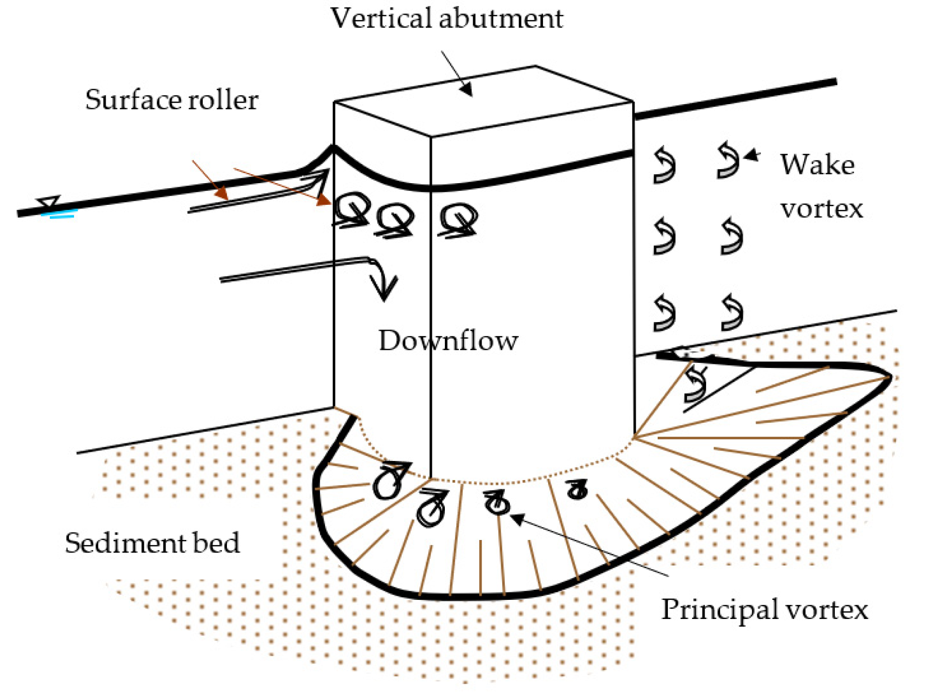
The basic mechanism causing local scour at bridge abutments is the formation of vortices at their base, as shown in Figure 1 [16]. The vortex moves bed material from the base of the abutment. If the outgoing rate of sediment transport is higher than the incoming rate, a scour hole forms. On the other hand, there are vertical vortices downstream of the structure called wake vortices. The force of wake vortices decreases rapidly while the distance downstream of the structure increases. Generally, the depths of local scour are much larger than general or contraction scour depths, often by a factor of ten [3].

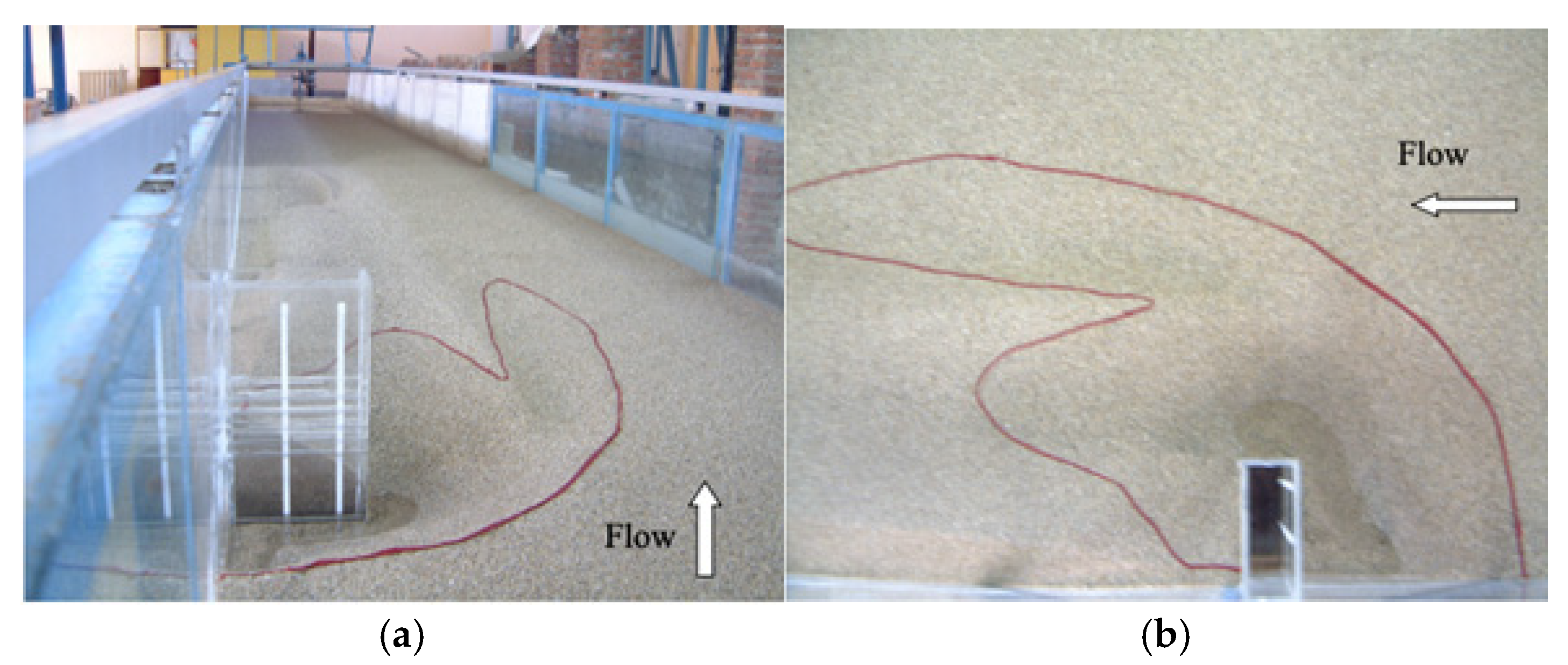
The abutment shape for all the experimental data analyzed in the present study was a vertical wall, and the equilibrium scour depth (Dse) and water depth (Y) measurement sections are shown in Figure 2.

An experimental test was conducted in the Technical Research and Quality Control Laboratory of the General Directorate of State Hydraulic Works for this study to visually show the local scour formation around bridge abutments. Figure 3 shows the formation of abutment scour obtained in the laboratory under the experimental conditions of B = 150 cm, L = 25 cm, V = 0.38 m/s, d₅₀ = 1.48 mm, and Dse of 10.2 cm. The 72 h scour hole formation obtained in this experimental study is shown in Figure 2.

2.2. Parameters Affecting Scour Around Bridge Abutments

Factors that affect the magnitude of local scour depth at abutments are given in Figure 4 [16]. Their definitions are given below:

• Flow velocity (V): As the flow velocity increases, the scouring force also increases. Therefore, data were collected in a wide range of velocities.
• Flow depth (Y): an increase in the flow depth can increase the scour depth by a factor of 1.1 to 2.15, depending on the abutment shape [3].
• Abutment length (L): the scour depth increases with an increasing abutment length.
• Bed material size and gradation: bed material characteristics such as gradation and cohesion can affect local scour.
• Abutment shape: as the streamlining shape of the abutment reduces the strength of the horseshoe vortex, the scour depth decreases.

2.3. Parameters Affecting Scour Around Bridge Structures

For clear water approach flow conditions, the equilibrium scour depth (Dse) at a support point is a function of the parameters given in Equation (1):

$$Dse=f\left\{L, B, V, Y, S, g, \rho s, \rho , \mu , d_{50}, \sigma g, t, B\right\}$$

(1)

where L = abutment length, B = abutment width, V = mean approach flow velocity, Y = flow depth, S = slope of the channel, g = gravitational acceleration, ρs = sediment density, ρ = fluid density, μ = dynamic viscosity of fluid, $d_{50}=$ median particle grain size, σg = (d₈₄/d₁₆)^0.5 geometric standard deviation of sediment size distribution (where d₈₄ = sediment size for which 84% of the sediment is finer, d₁₆ = sediment size for which 16% of the sediment is finer), and t = scouring time.

In terms of dimensionless parameters, the Dse can be described as Equation (2):

$${\displaystyle \frac{Dse}{Y}}=f\left\{{\displaystyle \frac{L}{Y}}, {\displaystyle \frac{B}{Y}}, {\displaystyle \frac{\rho s}{\rho }}, {\displaystyle \frac{Vt}{Y}}, {\displaystyle \frac{V}{\sqrt{gY}}}, {\displaystyle \frac{\mu }{V\rho Y}}, S, \sigma g, {\displaystyle \frac{d_{50}}{Y}}\right\}$$

(2)

If the bed slope, duration of the experiment, and viscous effects are ignored, one can simplify this as Equation (3):

$${\displaystyle \frac{Dse}{Y}}=f\left\{{\displaystyle \frac{L}{Y}}, {\displaystyle \frac{B}{Y}}, {\displaystyle \frac{V}{\sqrt{gY}}}, {\displaystyle \frac{d_{50}}{Y}}\right\}$$

(3)

where the equilibrium scour depth is normalized with flow depth.

2.4. Dataset

The dataset used in this study was created with experimental measurements and included various flow velocities, channel widths, and discharge features representing real-world hydraulic conditions [17]. The reason for the dataset being limited to 150 observations is that the data obtained in the experimental environment can be directly compared with field measurements. In addition, it has been shown that the features used (flow depth, abutment length, channel width, velocity, and median grain size) are compatible with the parameters commonly used in the hydraulic engineering literature. When access to larger datasets is provided, the generalization capacity of the models can be increased with transfer learning or data augmentation methods. Each observation in the dataset was recorded with digital measurement sensors and high-resolution cameras in a laboratory environment during the experiments.

This study achieves the evaluation and prediction of the results with various machine learning methods: Multiple Linear Regression, Support Vector Regression (SVR), Decision Tree Regressor, Random Forest Regressor, XGBoost, and Artificial Neural Networks (ANNs). The dataset used in this study contains 150 data records; 5 features, namely, Y (flow depth), L (abutment length), B (channel width), V (flow velocity), and $d_{50}$ (average grain size); and 1 class, i.e., Dse (equilibrium scour depth).

In the study, 150 experimental data belonging to the researchers given in

Table 1. Main characteristics of the experimental studies and limits of the experimental dataset.

Researchers	Dse (cm)	Y (cm)	L (cm)	B (cm)	d50 (mm)	V (m/s)	t (s)
[18]	13.41–39.82	9–18.30	5–20.2	20–193	0.5–0.19	0.44–0.72	285,900–3,809,820
[19]	14.71–39.87	2–35	16.5–30.2	80–152	0.082	0.27–0.36	177,442–358,699
[20]	11.1–41.04	10–60	15–30	152	0.09–1.8	0.33–1.43	223,569–899,163
[21]	5.52–44.12	12–20	30–60	240	0.08	0.21–0.28	275,848–590,975
[22]	5.52–18.33	10.67–13.29	15.2	91	0.14	0.21–0.26	1,155,397–3,355,840
[23]	4–28.9	4–14	10–30	200	0.14–0.58	0.22–0.70	4200–517,500
[24]	3.9–22.6	1.1–30	20	100	0.055	0.15–0.23	66,600–255,600

have been used and Table 1 shows the characteristics and measurement limits of the data groups. The maximum and minimum values of the experimental studies are given in Table 1.

2.5. Multiple Linear Regression

Multiple Linear Regression (MLR) is a statistical method used to model the linear relationship between the dependent variable and more than one independent variable [25]. Its main purpose is to estimate the dependent variable (Dse—equilibrium scour depth) using certain independent variables (Y, L, B, V, d₅₀). The MLR model has the general formula stated in Equation (4).

$$Dse={\beta }_0+{\beta }_{1}Y+{\beta }_{2}L+{\beta }_{3}B+{\beta }_{4}V+{\beta }_5{d}_{50} +\epsilon$$

(4)

where Dse is the desired equilibrium scour depth; Y, L, B, V, and $d_{50}$ are independent variables (hydraulic and sedimentological parameters); β₀ is the constant term (intercept) of the model; β₁, β₂, …, β₅ are the coefficients of each independent variable (weights learned by the model); and ε is the error term (variability that cannot be explained with the independent variables).

Multiple Linear Regression is trained using the Ordinary Least Squares (OLSs) method. This method determines the model coefficients by minimizing the sum of the squares of the error term. The following metrics are generally used to evaluate the performance of the model [25].

The Mean Square Error (MSE) is the average of the squares of the differences between predicted and actual values. The Root Mean Square Error (RMSE), the square root of the MSE, expresses the error size in the original measurement unit. The Coefficient of Determination (R²) shows how much the model explains the total variability in the dependent variable. It varies between 0 and 1; values close to 1 indicate that the model fits well.

The model is quite easy to interpret and apply. It offers the opportunity to analyze the effect of independent variables on the dependent variable separately. It can produce strong estimates, especially when it comes to linear relationships. If there is multicollinearity between independent variables, the reliability of the model may decrease. It cannot model nonlinear relationships well enough. Outliers and missing data can damage the model.

The MLR model will be compared with other machine learning models, and its accuracy in estimating the equilibrium scour depth will be evaluated in this study. The results will provide important information for comparing traditional linear methods with more advanced algorithms.

2.6. Support Vector Regression (SVR)

Support Vector Regression (SVR), unlike traditional regression methods, is a machine learning method that models the relationship between the dependent variable and the independent variables in line with the principles of Support Vector Machines (SVMs) [26]. SVR can map data into a high-dimensional space using kernel functions to increase the estimation performance in linear or nonlinear data. Instead of linear regression, SVR estimates by considering the data within the marginal error margin (ε-tube). The general formula for SVR is given in Equation (5).

$$f\left(X\right)=w^{T}X+b$$

(5)

where X is the vector of independent variables (Y, L, B, V, $d_{50}$), w is the weight vector, b is the constant term (bias) of the model, and f(X) is the estimated dependent variable value (Dse).

SVR uses the ε-insensitive loss function as the error function. This approach ignores errors that fall within a certain tolerance range ε and focuses only on minimizing estimates that fall outside this range. The function is shown in Equation (6) [27].

$$L_{\epsilon }\left(y,\hat{\mathrm{y}}\right)=\left\{\begin{array}{cc}\hfill 0,& \hspace{1em}if \left|y-\hat{\mathrm{y}}\right|\le \epsilon \hfill \\ \hfill \left|y-\hat{\mathrm{y}}\right|-\epsilon ,& \hspace{1em}otherwise\hfill \end{array}\right.$$

(6)

where ε is a hyperparameter that determines the sensitivity of the model. SVR can use kernel tricks to model nonlinear relationships. The most used kernel functions are as follows [27]:

• Linear Kernel: ⟨X_i, X_j⟩.
• Polynomial Kernel: (γ⟨X_i, X_j⟩ + r)^d.
• Radial Basis Function (RBF) kernel: exp(−γ║X_i − X_j║²).

In this study, the SVR model will be trained using the RBF kernel. The performance of the SVR model will be evaluated with the MSE, RMSE, and R² metrics. It can produce successful results even with small datasets. It is robust against noisy data and minimizes overfitting. It can model nonlinear relationships well, due to its kernel functions. The training time may be longer for large datasets. Model hyperparameters (ε, C, γ) should be carefully adjusted. To prevent over-learning in the SVR model and to obtain the best performance values, the grid search optimization method, RBF kernel, C (regularization) hyperparameter value of 10, and Epsilon (ε) hyperparameter value of 0.1 were selected. In this study, the SVR model will be compared with other machine learning algorithms, and its accuracy in estimating the equilibrium scour depth will be analyzed.

2.7. Decision Tree Regressor

Decision Tree Regressor (DTR) is a highly explainable machine learning model that uses a tree-based structure to predict the value of the dependent variable. The decision tree branches by dividing the independent variables according to certain threshold values and determining the predicted value at each leaf node. This method stands out due to its ability to model complex nonlinear relationships [28].

Decision Tree Regression applies a recursive partitioning process to the data using the independent variables in the dataset. The basic components of the model are as follows: nodes are partitioning operations that determine decision points, branches are connections representing different decision paths, and leaves are terminal nodes containing the final predicted values [29].

In Decision Tree Regression, the partitioning process is achieved by determining the best partitioning point for a given independent variable. The most common criterion used when determining the partitioning point is the MSE, shown in Equation (7). The data are divided into two subsets in a way that minimizes the MSE.

$$MSE={\displaystyle \frac{1}{n}}\sum _{i=1}^n{(y_i-{\hat{\mathrm{y}}}_i)}^2$$

(7)

where y_i is the real value and $\hat{y}$_i is the estimated value. The aim is to choose the best variable and value that minimizes the error rate at each split point.

It can model nonlinear relationships. It does not require data scaling (no need to normalize the features). It has high explainability, and decision processes can be visualized. The risk of overfitting is high, especially when deep trees are created. It is sensitive to data noise; small changes can lead to different decision trees. Its generalization ability is limited, so it is often supported by ensemble learning methods such as Random Forest.

The performance of the model will be evaluated with the MSE, RMSE, and R² metrics. In this study, Decision Tree Regression will be used to evaluate the accuracy in estimating the equilibrium scour depth (Dse) by comparing it with other machine learning methods. To prevent over-learning in the DTR model and to obtain the best performance values in the manual tuning optimization method, the maximum depth hyperparameter and the minimum sample split values were selected 4 and 2, respectively.

2.8. Random Forest Regressor

Random Forest Regressor (RFR) is an ensemble learning method based on decision trees. It creates a more powerful and generalized model by combining the predictions of multiple decision trees instead of a single decision tree. This approach reduces the risk of overfitting and increases the accuracy of the model [30].

Random Forest averages the outputs of many decision trees created using the Bootstrap Aggregation (bagging) method. The main steps of the model are sampling (Bootstrapping), training the trees, and making predictions [31].

The Random Forest model provides a more balanced prediction process by reducing the high variance (overfitting tendency) of individual decision trees.

A Random Forest model is created by averaging the outputs of M number of decision trees and is calculated with Equation (8).

$$\hat{\mathrm{y}}={\displaystyle \frac{1}{M}}\sum _{m=1}^M{f}_m\left(X\right)$$

(8)

where $\hat{y}$ is the final estimate, M is the total number of decision trees, and f_m(X) is the estimate of the mth decision tree.

Each decision tree uses the MSE criterion to determine the best split point for a given feature. The aim here is to select the feature that minimizes the error rate at each split step.

It is resistant to over-learning (due to the bagging method) and can model nonlinear relationships well. It can also determine the order of importance of features, i.e., show which variable has more effect on the model. However, the training time is long, especially when many decision trees are trained on large datasets; its interpretability is low because the decision mechanism becomes difficult to understand since many trees are averaged; and the computational cost may increase when too many trees are used [31].

The performance of the Random Forest model will be evaluated using the MSE, RMSE, and R² metrics. Random Forest Regressor will be used to estimate the equilibrium scour depth (Dse) around bridge side abutments by comparing it with other regression models in this study.

2.9. XGBoost

XGBoost (Extreme Gradient Boosting) is a powerful ensemble learning method based on decision trees. Based on the boosting principle, this model provides high accuracy and a low error rate by using an ensemble of weak estimators (decision trees). It is widely preferred in regression and classification problems due to its fast, scalable, and optimized structure [32].

The XGBoost model is a gradient boosting technique that tries to minimize the error rate by using successively trained decision trees. In the model, the initial estimate is made by first taking the average of the target variable (Dse). The difference between the true value and the estimated value (residual) is calculated for each sample. To reduce the error rate, the model trains each new decision tree to correct the prediction errors of the previous model. Each new tree is added to the previous predictions with a certain weight (α). This process continues until the specified number of decision trees is created. Since each new tree is trained to correct the errors of the previous model, the accuracy of the model increases [33].

The XGBoost model learns by minimizing the loss function. The general formula of the model is as shown in Equation (9).

$$\hat{\mathrm{y}}=\sum _{m=1}^M{f}_m\left(X\right)$$

(9)

where y is the model’s prediction for the ith data point, M is the total number of decision trees used in the model, and fm(X) is the prediction value produced by the mth decision tree. Each new tree is trained according to the derivative of the loss function using the Gradient Descent principle. The loss function is optimized using the second-order Taylor approximation to reduce the error rate and is shown in Equation (10).

$$L^t=\sum _{i=1}^n{l(y_i,{{\hat{\mathrm{y}}}_i}^{\left(t-1\right)}+f}_t\left(X_i\right))+\mathsf{\Omega }(f_t)$$

(10)

where L^(t) is the total error at iteration t, L(y, $\hat{y}$) MSE, and $\mathsf{\Omega }\left(f_t\right)$ is the complexity penalty function of the model (regularization).

This optimization process creates a mechanism that prevents overfitting while reducing the error rate. Due to the boosting method, model errors are systematically corrected. The generalization of the model is provided with the L1 and L2 regularization techniques. It works effectively on large datasets, because of its ability to perform parallel processing. The model can show which variables are more important in the estimation process. Parameters such as the learning rate and max depth should be carefully selected for the performance of the model. The computational cost may increase at large tree depths [34].

The MSE, RMSE, and R² metrics will be used to measure the performance of the XGBoost model. XGBoost Regressor will be used to estimate the equilibrium scour depth (Dse) around bridge side abutments by comparing it with other regression models in this study. To prevent over-learning in the XGBoost model and to obtain the best performance values in the random search optimization method, the learning rate hyperparameter, the max depth hyperparameter and the number of trees were selected 0.05, 6, and 100, respectively.

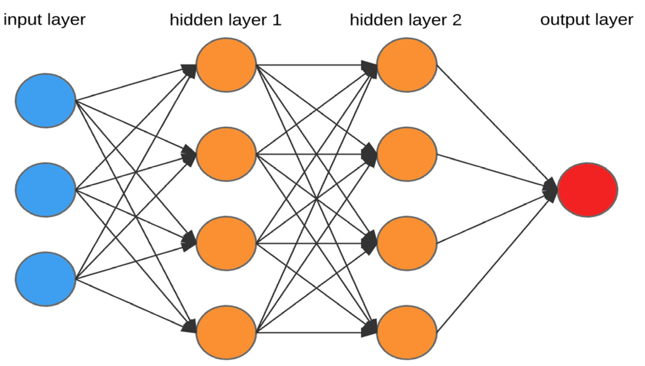
2.10. Artificial Neural Networks

Artificial Neural Networks (ANNs) are powerful machine learning models that perform tasks such as data analysis, prediction, and classification based on the working principles of neurons and synapses in the human brain [35]. ANNs, which form the basis of deep learning techniques, can make high-accuracy predictions with large and complex datasets. The simplest processing unit in an Artificial Neural Network is a single-layer perceptron called a neuron (see Figure 5) [36].

An Artificial Neural Network consists of three basic components: the input layer, hidden layers, and output layer. The features in the dataset are processed in the input layer and transferred to the model [37]. In the hidden layer, each neuron processes the weighted sum it receives from the inputs connected to it through an activation function. The final prediction value is produced in the output layer. The multilayer perceptron model works by progressing from the input layer to the output layer, as shown in Figure 6 [36].

The activation of each neuron (a = f(z)) is calculated using Equation (11).

$$z=\sum _{i=1}^n{w}_i{x}_i+b$$

(11)

where w_i is the weight values, x_i is the input values, b is the bias term, f(z) is the activation function, and a is the output obtained as a result of activation.

In ANN models, activation functions increase the learning capacity of the network by providing a nonlinear transformation of the input. Common activation functions are the ReLU, Sigmoid, and Tanh (Hyperbolic Tangent) functions. In this study, the ReLU function (f(x) = max(0, x)) is preferred because it enables the model to learn faster by zeroing out negative values and minimizes the vanishing gradient problem [38].

ANN models are trained with Backpropagation and Gradient Descent algorithms. The Forward Propagation method passes input data through neurons to create predictions [39]. The error between the true values (Dse) and the predicted values is determined. The Backpropagation method updates the error by distributing it to the weights and bias terms with chained derivative calculations. With the Gradient Descent method, the weights are updated according to the learning rate (a) using Equation (12).

$$w_{new}=w_{old}-\alpha {\displaystyle \frac{\vartheta L}{\vartheta w}}$$

(12)

where L is the loss function (i.e., Mean Square Error—MSE), a is the learning rate, and w is the weights of the model. This process continues for a certain number of iterations (epochs), and the model is trained until the error rate is minimized.

It can learn complex relationships and successfully model nonlinear structures. It reduces the need for feature engineering because it can perform automatic feature extraction. It can work effectively on large datasets with parallel computation. The computational cost is high because large network structures require high processing power. It is prone to overfitting so regularization techniques are required. Hyperparameter tuning is difficult; therefore, extensive experiments are required for the optimum structure.

The performance of the ANN model will be evaluated with the MSE, RMSE, and R² metrics. The ANN model will be used to estimate the equilibrium scour depth (Dse) around bridge side abutments by comparing it with other regression models in this study. To prevent over-learning in the ANN model and to obtain the best performance values in the grid search optimization method, the ReLU as the activation function the number of layers and the learning rate 3, and 0.01, respectively.

3. Results

In this study, different regression models were applied and evaluated to estimate the equilibrium scour depth (Dse) around bridge abutments.

The following preprocessing steps were applied before the data were entered into the model:

• Statistical analysis was used to check whether there were any mistakes or incorrect entries in the dataset. Observations with less than 5% missing data were filled with the mean, and observations with more missing data were excluded from the analysis.
• Min-Max Normalization was applied for Support Vector Regression (SVR) and Artificial Neural Network (ANN) models. Scaling was not deemed necessary for Random Forest and Decision Trees.
• Extreme values were determined with the Interquartile Range (IQR) method, and extreme points were removed from the dataset.
• To increase the model accuracy, the dataset was divided into 80% training and 20% testing. A 5-fold cross-validation method was used to prevent the over-learning of the models.
• Correlation analysis and SHAP (SHapley Additive Explanations) values were calculated to determine the effect of the features on the model. Variables with a correlation coefficient of less than 0.1 were not used in model training. To increase model performance, the most important features were determined with the Recursive Feature Elimination (RFE) method. Thanks to these steps, the dataset was purified from noise and made modelable, and the generalization success of the model was increased.

The dataset used in the machine learning models was divided into 80% model training and 20% testing. Each of the models was trained using training data, and testing was performed using test data. The MSE, RMSE, MAE, MAPE, and R² metrics were used to evaluate the performance of machine learning models. The MSE is the average of the squared differences between the actual values and the predicted values. This error metric measures how successful the model is in making correct predictions. The RMSE is the square root of the MSE and takes the square root of the average of the differences between the actual values and the predicted values. Therefore, the biggest difference between the RMSE and MSE is that it acts, metaphorically speaking, like a punisher by giving more weight to large errors with this mathematical operation; on the other hand, it rewards very small errors. The R² is a measure of the agreement between the actual value and the model’s predictions. It is found by dividing the variance of the actual values by the variance of the predicted values. The R² value takes a value of between 0% and 1%, and a value of 1% means that the model explains the data perfectly and the model fits perfectly. The MAE (Mean Absolute Error) shows the average error amount of the model, while the MAPE (Mean Absolute Percentage Error) shows the percentage error amount. The metrics of the models are shown in

Table 2. Performance metrics of machine learning models.

Model	MSE	RMSE	MAE	MAPE	R2	Accuracy	Training Time (s)
MLR	25.006	5.000	4.21	12.3%	0.806	81.14%	13.56
SVR	36.525	6.043	5.12	15.6%	0.894	86.47%	14.85
DTR	4.656	2.157	1.32	3.5%	0.992	99.28%	4.35
RFR	10.480	3.237	2.10	7.8%	0.972	95.63%	6.54
XGBoost	5.461	2.336	1.89	4.2%	0.990	99.21%	5.29
ANN	8.708	2.950	2.50	6.5%	0.981	98.77%	12.78

.

When the metrics of the models in this table are examined, it can be seen that the best performance values were achieved by the DTR (99.28%), XGBoost (99.21%), ANNs (98.77%), and RFR (95.63%) machine learning models. With these models, predictions with high accuracy rates were made using test data. The DTR model performed better on small datasets because of less overfitting, faster generalization due to the simple structure of the model, and sometimes increased complexity due to the extreme parameter sensitivity of ANNs and XGBoost. This suggests that decision trees may have an advantage for small datasets.

The hydraulic and sedimentological parameters used in this study are widely accepted variables in hydraulic engineering. The parameter selection was based on experimental and field studies in the previous literature. The compatibility of the results obtained from both experimental and field methods was taken into consideration when selecting the parameters.

A simulator application code was written for the DTR model that showed the highest performance value, and testing was performed on it, as shown in Figure 7. For the testing process, the values of 9.48, 10.0, 60, 0.500, and 0.64 were entered for the Y, L, B, $d_{50}$, and V features, respectively, and the equilibrium scour depth (Dse) value around bridge abutments was estimated as 23.450. It was determined that the estimated value had a high accuracy rate. The predicted values of all models used in this study are shown in

Table 3. Estimated Dse values for new data.

Model	Dse
MLR	19.587232
SVR	21.548026
DTR	23.450000
RFR	23.181600
XGBoost	23.452053
ANN	23.692532

.

As shown in Table 3, the DTR (23.450 cm) and XGBoost (23.452 cm) models have the highest accuracy rate in terms of the estimated scour depth. This shows that these models can provide high accuracy with small datasets and decision tree-based algorithms are generally more successful in scour prediction. The ANN model gave the highest estimated value (23.693 cm) compared to the other models. This may indicate that ANNs give more weight to some extreme values in the data generalization process. In addition, it is known that ANNs generally perform better with large datasets and can sometimes overestimate with small datasets.

The SVR model (21.548 cm), although it has the ability to learn nonlinear relationships in particular, did not perform as well as DTR and XGBoost on this dataset. The MLR model (19.587 cm) gave the lowest estimate, which shows that the linear regression method is limited in modeling such complex hydraulic problems. The Random Forest Regressor (RFR) model (23.182 cm) showed a similar performance to other tree-based models. The results of XGBoost and DTR models are very close to each other. This shows that these models have similar decision mechanisms due to their nonparametric nature.

DTR and XGBoost showed the best performance, indicating that these models can provide reliable predictions in engineering projects. ANNs can be more successful for large datasets but should be carefully tuned for small datasets. Linear models such as SVR and MLR show limitations in modeling complex hydraulic processes and should only be used for simple scenarios.

The predictions presented in Table 3 confirm that DTR and XGBoost based on decision trees are the best models for scour depth prediction. Future testing of these models with field data can increase their reliability in engineering applications. It is suggested that the performance of ANNs should be improved when trained with larger datasets, considering their high predictions.

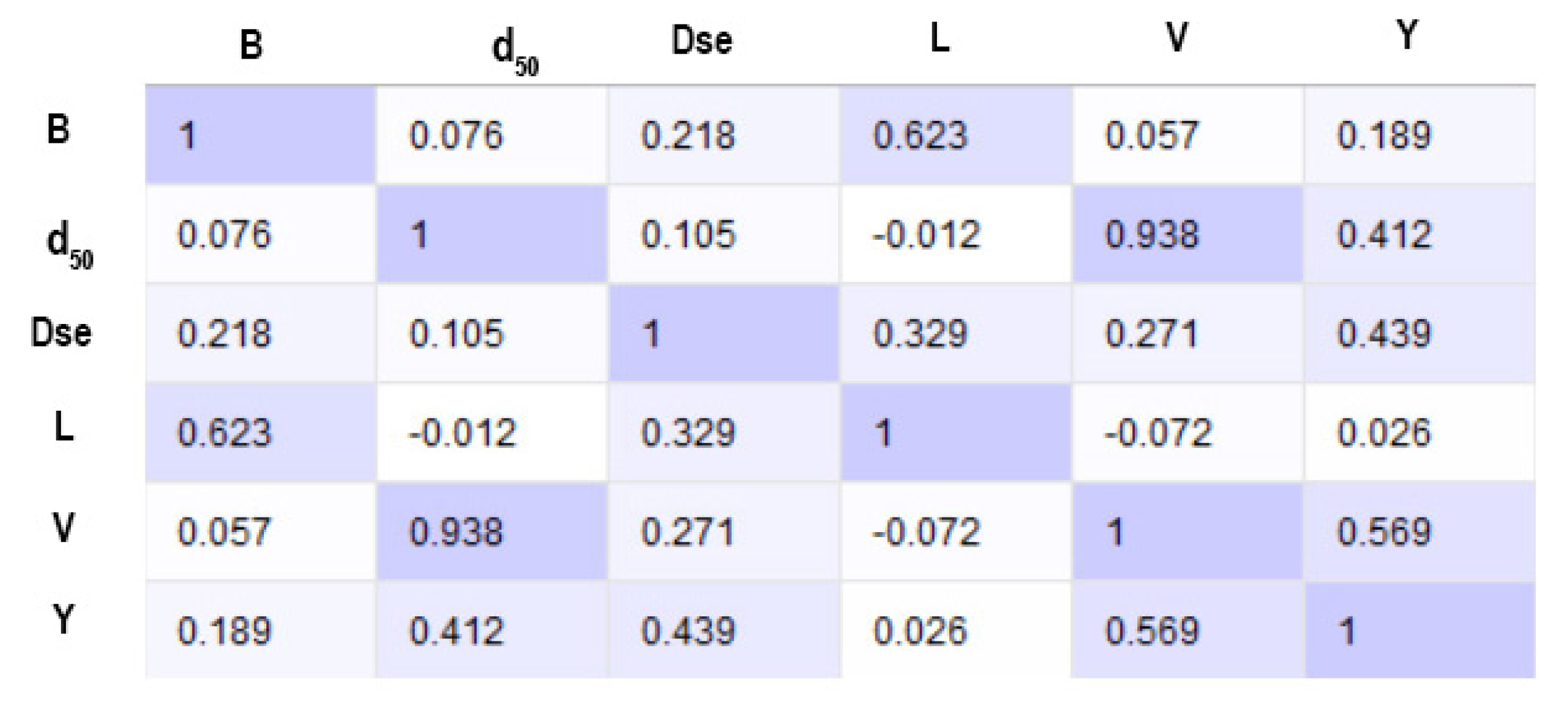
The correlation distribution matrix of the features in the dataset is shown in Figure 8. The correlation matrix shows the relationships between the features and their effects on each other.

The correlation coefficient between the flow depth (Y) and equilibrium scour depth (Dse) was calculated as r = 0.439. This positive correlation shows that an increasing flow depth is directly related to a greater scour depth. This finding is consistent with the results given in the literature and the hydraulic principles.

The correlation coefficient between the abutment length (L) and Dse is r = 0.329. This indicates that increasing the side foot length increases the scour depth. Especially long side feet can increase turbulent flow and cause deeper scours. A correlation of r = 0.218 was observed between the channel width (B) and Dse. As the channel width increases, the scour depth is expected to decrease. This is because wide channels provide flow dispersion and reduce turbulence intensity.

The correlation between the flow velocity (V) and Dse is at a low level of r = 0.221. Although it is generally thought that higher flow velocities lead to larger scours, this study shows that flow velocity alone is not a determining factor. This low correlation suggests that the effect of flow velocity on scour should be evaluated together with other factors such as the flow depth, side foot length, and channel width. The correlation between the median grain size ($d_{50}$) and Dse (r = 0.105) shows that the scour depth decreases as the grain size of the soil material increases. Larger-grained soils may cause shallower scours because they offer more resistance to flow.

Variables with high correlation coefficients (Y and L) were determined as the most important features to improve model performance. The B and $d_{50}$ variables can be considered as balancing factors for the scour process. The weight of variables with low correlation, such as the flow velocity (V), may need to be optimized in the model. The flow depth (Y) and abutment length (L) are the most critical variables in scour depth estimation. The channel width (B) and median grain size ($d_{50}$) play a role as limiting factors for scour depth. The low correlation between the flow velocity (V) and Dse indicates that this parameter alone is not a strong predictor. In future studies, model configurations that give weight to the strongest variables determined by correlation analysis should be preferred.

As seen in Figure 9 and

Table 4. Feature importance scores for Random Forest and XGBoost models.

Feature	Random Forest	XGBoost
V	0.373246	0.397831
L	0.274575	0.240758
d50	0.073092	0.180270
Y	0.257486	0.140714
B	0.021601	0.040427

, the flow rate (V) has the highest importance score in both the Random Forest (37.32%) and XGBoost (39.78%) models. This shows that the flow rate is the most decisive variable in estimating the scour depth (Dse). The abutment length (L) has an importance score of 27.46% in the Random Forest model and 24.08% in the XGBoost model. This proves that the length of the bridge pier has a significant effect on scour depth. The average grain size ($d_{50}$) has an importance score of 18.03% in the XGBoost model, while it has a low score of 7.31% in the Random Forest model. This shows that its contribution to the estimation may vary depending on the model. The flow depth (Y) has an importance score of 25.75% in the Random Forest model and 14.07% in the XGBoost model. The fact that XGBoost gives less weight to this variable indicates that the model is more dependent on certain variables. The channel width (B) has the lowest importance score (Random Forest: 2.16%, XGBoost: 4.04%). This reveals that the channel width is less effective than other variables in terms of scour depth estimation.

The fact that the XGBoost model gives more weight to the $d_{50}$ variable shows that the model considers sedimentological factors more. The Random Forest model considers the flow depth (Y) to be a more important variable. The flow velocity (V) and abutment length (L) are the most important factors in both models and play a critical role in scour depth estimation. The fact that $d_{50}$ is considered more important by XGBoost shows that the model is sensitive to sediment properties, but Random Forest gives less importance to this variable. The channel width (B) has the lowest importance score in both models, which shows that width may have a limited effect on scour depth.

Performance comparisons of the models using the MSE, RMSE, and R² metrics are shown in Figure 10. As can be seen from the graphs, the model that best performs the prediction process with the dataset used is the Decision Tree Regression model.

DTR and XGBoost have the lowest error and highest R² values. DTR achieved the lowest MSE (4.656), RMSE (2.157), and highest R² (0.992) values. The XGBoost model shows very close performance to DTR (MSE: 5.461, RMSE: 2.336, R²: 0.990). These results confirm that decision tree-based algorithms (such as DTR and XGBoost) are quite successful, especially with small datasets. XGBoost balances overfitting better thanks to the boosting mechanism that increases generalization ability.

The ANN, although it shows a successful performance, falls behind DTR and XGBoost. The ANN showed a very good performance with an MSE of 8.708, an RMSE of 2.950, and an R² of 0.981. However, since the ANN model has a structure that requires more data than other models, it was not as successful as DTR and XGBoost with small datasets. It is estimated that the performance of ANNs can be further increased when working with large datasets.

Random Forest showed good performance but fell behind XGBoost and DTR. RFR exhibited a strong prediction performance with an MSE of 10.480, an RMSE of 3.237, and an R² of 0.972. However, the XGBoost model, despite using the same tree-based structure, reached lower error rates thanks to the boosting mechanism. This shows that XGBoost generalizes better by balancing over-learning even in small datasets.

The SVR and MLR models have higher error rates. The SVR model has a higher error rate compared to other models with an MSE of 36.525, an RMSE of 6.043, and an R² of 0.894. MLR showed the lowest performance (MSE: 25.006, RMSE: 5.000, R²: 0.806). This result reveals that traditional statistical approaches are inadequate for complex, nonlinear problems such as scour depth estimation. The failure of SVR shows that kernel-based approaches may not work very well with small datasets and require more parameter optimization.

DTR and XGBoost can be considered as reliable models for scour depth estimation in engineering projects. The ANN model can provide higher accuracy when the dataset is enlarged or when transfer learning techniques are applied. Traditional methods such as SVR and MLR alone are not sufficient for hydraulic engineering problems because they cannot adequately capture nonlinear relationships. Although Random Forest is a good option in terms of overall performance, it makes more errors since it does not have optimization mechanisms like XGBoost.

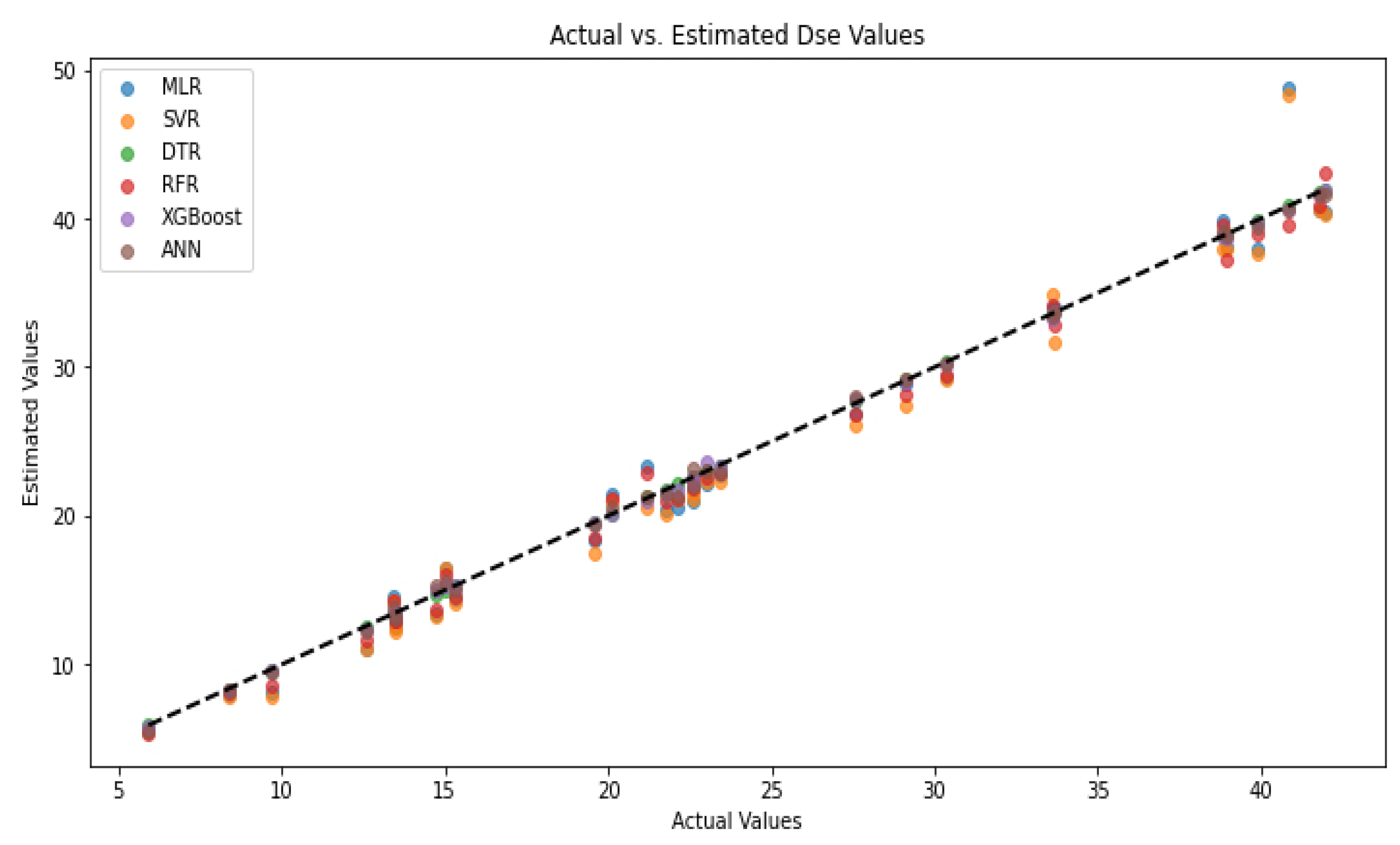
Figure 11 visualizes the relationship between the scour depths (Dse) predicted by different machine learning models and the actual measured values. The graph compares the observed and predicted values to evaluate the models’ prediction accuracy.

DTR and XGBoost predicted with the lowest error. DTR and XGBoost provided the best model with predictions that almost matched the actual values. The predicted points for the DTR model were well aligned with the actual values, indicating that the model provided an excellent fit even with small datasets. The XGBoost model also showed a similarly strong performance, producing predictions with low error rates.

RFR is close to the actual values but shows slight deviations. Although the RFR model provides a good fit overall, it shows slight deviations at some extreme points. It is seen that RFR makes some over- or under-predictions, especially at higher Dse values. These deviations may be because Random Forest cannot fully learn some complex relationships due to the bootstrap sampling method.

The ANN model was close to the true values but slightly unstable. The ANN model generally made predictions close to the true values, but there were significant differences at some extreme values. It was observed that the ANN tended to deviate slightly from the true value, especially at high Dse values. This may be due to the ANN’s hyperparameter sensitivity and overfitting tendency with small datasets.

The SVR and MLR models made more errors. The SVR and MLR models had larger prediction errors, especially at high Dse values. Although SVR provided predictions quite close to the true values in some cases, it showed serious errors, especially at the low and high ends. The MLR model had the lowest accuracy and deviated greatly from the true values. This shows that complex, nonlinear relationships such as scour depth cannot be adequately represented by simple regression models.

The excellent fit of the DTR and XGBoost models showed that these models can provide reliable predictions in field studies. Although RFR and ANNs had low error rates, they need further optimization in some cases. SVR and MLR were insufficient to provide reliable estimation in complex physical processes such as hydraulic engineering. When selecting a model, it was recommended that DTR and XGBoost be preferred, especially in large infrastructure projects.

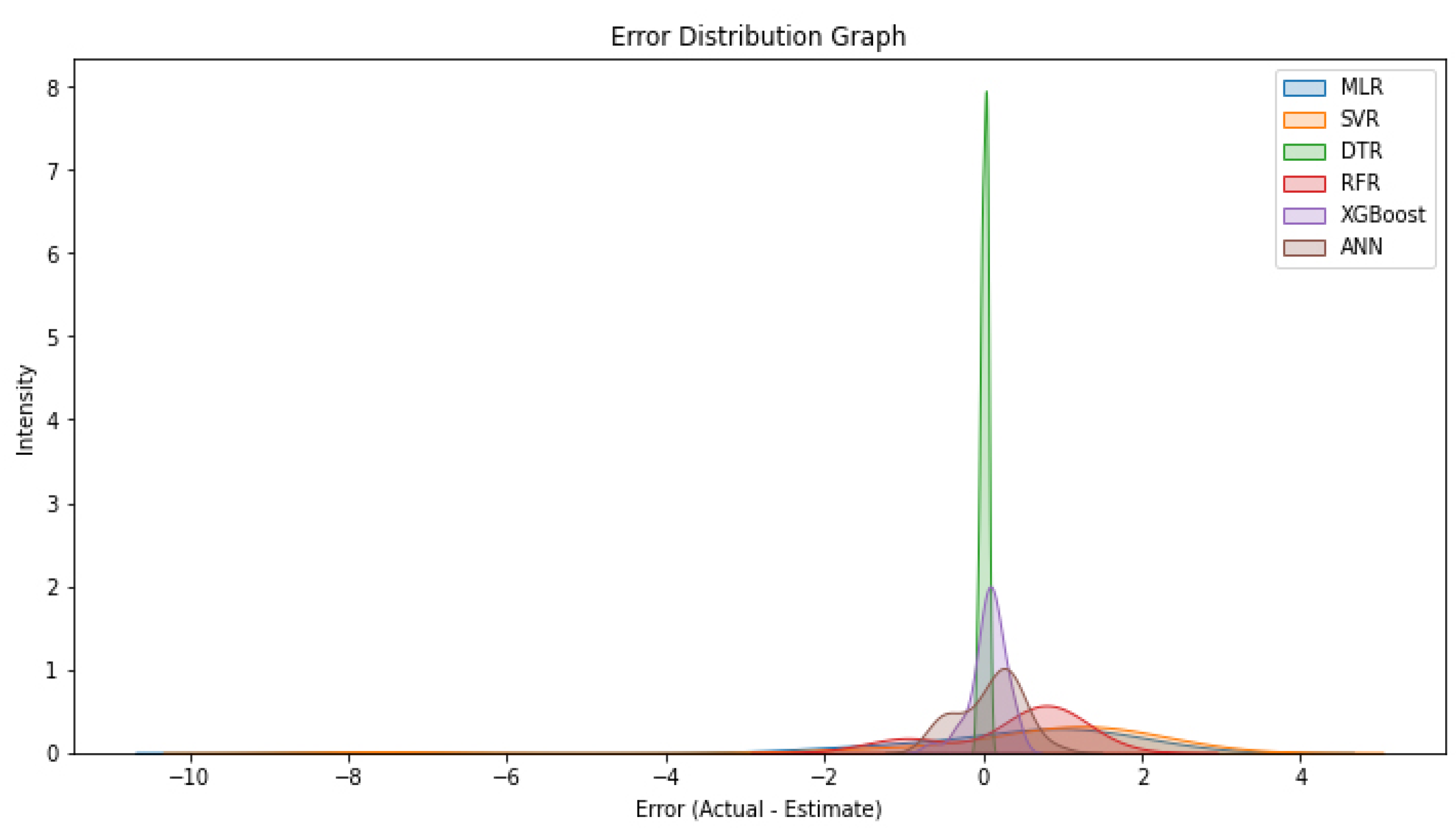
Figure 12 visualizes the error distribution of different machine learning models in scour depth (Dse) estimations. This graph plays a critical role in analyzing how the error rates of the models vary, which models make more consistent predictions, and which models show larger error deviations.

The DTR and XGBoost models have the smallest error distributions. DTR and XGBoost have the lowest error rates and the narrowest error distributions. This shows that DTR and XGBoost have strong prediction capabilities even with small datasets and do not show large error deviations. In particular, the DTR model stands out as the most reliable model by keeping the majority of the prediction errors within the ±2 cm range. XGBoost, on the other hand, provides more balanced predictions thanks to optimization mechanisms that minimize overfitting.

RFR has a balanced but slightly wider error range. Although the RFR model has mostly low error rates, it shows prediction deviations at some extreme values. In particular, it has been observed that there are some cases where the model makes errors greater than 5 cm, which indicates that the model is less reliable for certain observations. This situation reveals that the RFR model can generalize without over-learning, but in some cases, it can overestimate or underestimate.

The ANN model shows larger deviations at the extreme points. Although the ANN model generally makes good predictions, it made errors greater than 5 cm in some observations. This shows that the ANN may tend to over-learn with small datasets, and its errors increase in certain cases. When trained with large-scale datasets, the error distribution of the ANN can be narrowed, and it can be made to produce more consistent predictions.

The SVR and MLR models have the highest error distribution. It is observed that the error values are spread over a wide range and there are large prediction errors, especially in the MLR model. The SVR model also shows large deviations from time to time: it was observed that it overestimates at low Dse values and underestimates at high Dse values. This situation reveals that SVR and MLR are inadequate in modeling complex hydraulic problems.

The DTR and XGBoost models are the models with the lowest estimation errors and the highest reliability. The RFR model stands out as a model that does not make large errors but shows deviations from time to time. ANNs can reduce error rates when the dataset is expanded, but they shows some extreme deviations with small datasets. SVR and MLR fail to represent nonlinear relationships such as scour prediction in engineering applications.

4. Discussion

This study investigated the estimation of the equilibrium scour depth (Dse) around bridge abutments using various artificial intelligence (AI) models, including Multiple Linear Regression (MLR), Support Vector Regression (SVR), Decision Tree Regressor (DTR), Random Forest Regressor (RFR), XGBoost, and Artificial Neural Networks (ANNs). The results indicate that AI-based methods, particularly ensemble learning models and deep learning techniques, offer significant improvements over traditional regression approaches in terms of predictive accuracy and generalization capabilities.

One of the key findings of this study is that the Decision Tree Regressor (DTR) model achieved the highest accuracy (99.28%) in predicting the Dse, closely followed by XGBoost (99.21%) and ANNs (98.77%). These models demonstrated superior performance due to their ability to capture complex nonlinear relationships between the hydraulic parameters and scour depth. Traditional statistical models such as MLR, which rely on linear assumptions, were observed to have lower accuracy, emphasizing the necessity of more advanced machine learning techniques for such predictive tasks.

The superiority of ensemble learning techniques, such as Random Forest and XGBoost, can be attributed to their robust handling of high-dimensional data and ability to mitigate overfitting by aggregating multiple decision trees. Similarly, the ANN model, leveraging deep learning principles, exhibited strong generalization performance by efficiently learning patterns within the dataset. However, its slightly lower accuracy compared to tree-based methods suggests that feature selection and hyperparameter tuning could further enhance its performance.

Despite their high predictive power, AI models also have certain limitations. Computational complexity and training time were observed to be key challenges, particularly for the ANN and XGBoost models. The need for large datasets to achieve reliable generalization is another consideration, as data sparsity may lead to reduced performance in real-world applications. Furthermore, while AI models provide accurate predictions, they do not inherently offer physical insights into the scour process, which remains a crucial aspect of hydraulic engineering.

A comparison with experimental measurements showed a strong correlation between the observed and predicted values, reinforcing the validity of AI-based scour depth estimation methods. The application of AI models in bridge design and maintenance planning presents a promising avenue for future research, particularly in integrating real-time monitoring data with predictive analytics to enhance structural safety.

The limitations of previous studies include the low interpretability of AI models (especially ANNs, which act like a black box), the high risk of overfitting (with small datasets especially, complex models like ANNs and XGBoost may have generalization problems), and the lack of integration with physical models (AI models are not directly based on hydraulic theories; they only learn from data). This study focuses on making the model more transparent by performing feature importance ranking and correlation analysis.

Future studies could explore hybrid AI models that combine physical modeling principles with data-driven approaches to improve interpretability while maintaining high accuracy. Additionally, extending the dataset with more diverse hydraulic conditions and optimizing model architectures through automated machine learning (AutoML) techniques could further refine prediction capabilities.

Overall, this study highlights the potential of AI-driven methodologies in hydraulic engineering and infrastructure safety, providing a reliable and efficient alternative to conventional scour estimation techniques. The integration of such advanced computational models in practical engineering applications can significantly enhance decision-making processes, ultimately contributing to more resilient and sustainable bridge designs.

5. Conclusions

This study demonstrated the effectiveness of artificial intelligence models in predicting the equilibrium scour depth (Dse) around bridge abutments. Among the models tested, Decision Tree Regressor (DTR), XGBoost, and Artificial Neural Networks (ANNs) achieved the highest accuracy, indicating that machine learning techniques can significantly improve the estimation of scour depth compared to traditional empirical methods.

In this study, it was shown that AI-based models (DTR, XGBoost, ANNs, etc.) provide higher accuracy compared to traditional empirical equations. The DTR model provided the highest accuracy (99.28%), followed by XGBoost (99.21%) and ANNs (98.77%). Traditional empirical equations and the MLR model lagged behind AI methods in terms of accuracy.

It was determined that AI models better captured the complex, nonlinear relationships between the inputs, thus providing a more reliable alternative in scour depth estimation. The most important inputs of the model were determined with correlation analysis and SHAP value calculations, and the effect of these inputs on scour depth was revealed.

The dataset used in this study was limited to 150 records. The generalization ability of the models can be tested better with a larger dataset. Since AI models offer data-driven approaches that are not based on physical mechanisms, they do not provide a complete physical explanation from an engineering perspective. Laboratory data were used in this study; the performance of the models was not compared with real-world data collected in the field. The parameter tuning and hyperparameter optimization of AI models can be computationally costly, and the models’ accuracy may vary under different conditions.

The results are consistent with the studies by [4,5], which also showed that AI models are successful for scour depth estimation. Although the empirical formulas proposed by [2] are valid for certain hydraulic conditions, AI models provide higher accuracy in scenarios with wider variations. Hamidifar [7] reported that hybrid methods using empirical formulas and AI models together are successful. In the current study, only AI methods were examined, and hybrid models can also be evaluated in the future.

While some literature studies (e.g., [8]) indicated that ANN models showed the highest performance, the DTR model gave better results in this study. This difference may be due to the dataset, model parameters, and optimization methods used.

This study demonstrates that AI models provide a powerful alternative for estimating the equilibrium scour depth. However, hybridizing AI methods with empirical models, testing them with real field data, and improving their generalizability to larger datasets is an important step for future research.

The findings highlight the potential of AI-driven approaches for enhancing bridge safety by providing reliable scour depth predictions. These models successfully captured the nonlinear relationships between hydraulic and sedimentological parameters, offering an effective alternative to conventional regression-based techniques. The integration of AI into hydraulic engineering can contribute to improved infrastructure design, early risk assessment, and cost-effective maintenance strategies.

While AI models provide high accuracy, certain challenges remain, such as computational complexity, the need for large datasets, and interpretability issues. Future research should focus on optimizing model architectures, incorporating hybrid AI/physical modeling approaches, and utilizing real-time monitoring data to refine predictive capabilities.

In conclusion, this study underscores the transformative impact of artificial intelligence in hydraulic engineering. The use of advanced machine learning models can provide more accurate, efficient, and data-driven solutions for scour depth estimation, ultimately contributing to safer and more resilient bridge structures.