1. Introduction
The water demand of a city is influenced by various consumer groups, with the per capita water consumption of residents playing a significant role. Per capita water consumption is influenced by various factors, such as income, age, level of education, household size, and outdoor use (such as swimming pools and gardens) [
1,
2,
3,
4,
5,
6,
7] and there are several studies investigating these influencing factors [
8,
9,
10]. For example, Cominola et al. [
9] classify these factors into three key categories: external (e.g., weather), latent (e.g., behaviors, attitudes), and observable (e.g., age, income). These three categories are often analyzed together.
A study [
11] of 600 German supply areas identified income, household size, price, and age as key determinants. The results show that larger households consume less water per capita, while age and precipitation lead to higher consumption, and that temperature has no significant effect. Another study [
12] introduced a multi-level analysis of water demand by integrating household level data and aggregate data through panel data models. The study found that higher income households and those with a swimming pool were more influenced by weather conditions, and that both income and household size increase water consumption.
Costa et al. [
13] point out that water consumption of households is influenced by different factors, and local characteristics should be taken into account. Based on survey data, it was found that income, family size, and the presence of children have a significant influence on water consumption. Garcia et al. [
5] found that a higher level of education correlates with lower per capita water consumption. Rathnayaka et al. [
14] found that per capita water consumption in detached houses is 13% higher than in semi-detached houses and 26% higher than in multi-story buildings, primarily due to the presence of swimming pools and gardens. Additionally, a study [
15] found that households with a personal interest in gardening tend to have higher water consumption.
As shown in previous studies, per capita water consumption depends on various factors that can affect it differently across regions. However, it is important for water utilities to estimate local per capita water consumption and how different factors impact this consumption [
13]. According to the EU directive [
16], consumers should receive information at least once a year about their water consumption, its evolution, a comparison with the average consumption of other households, and the price per liter in order to better understand the impact of their consumption. For developing regions in particular, such initial values are necessary for water utilities to be able to estimate future demand. However, per capita consumption calculation requires data on registered residents per building, which are often unavailable due to data protection laws.
To address this, several studies have explored GIS-based approaches to estimating population at the building level [
17,
18,
19]. For example, one study [
17] used high-resolution aerial imagery and GIS data to extract building footprints and heights, identify residential buildings, and distribute the population accordingly. In another study [
20], the nighttime population distribution was estimated using building heights from satellite imagery and GIS data, achieving high accuracy in urban areas. This study [
18] integrated LiDAR data, POI, and nighttime light information into a random forest model, where building volume was identified as the most important factor for population distribution. A data-driven approach [
21] classified buildings using pattern recognition and machine learning based on e.g., digital landscape models, topographic raster maps, or cadastral databases. In addition, a study [
22] investigated the occupancy of buildings in low-income countries using GIS and machine learning based on satellite images. An ensemble model achieved an accuracy of 85–93% in distinguishing between residential and non-residential buildings. Another study [
23] presents a method for estimating static and dynamic population densities in large cities that is based on mobile phone metadata.
Some water utilities in Austria do not have access to registered resident data due to current data protection regulations. At the same time, accurate estimates of per capita water consumption by residential building type are essential for demand forecasting and infrastructure planning. However, many existing studies that estimate water consumption are based on direct access to demographic data, which are often unavailable for privacy reasons. Additionally, many population assessment approaches use complex methods to estimate the number of residents or use data, for example mobile phone data, that are not applicable or available for practitioners at utilities. This gap highlights the need for alternative approaches to estimate the number of residents in a building without relying on limited datasets. To address this challenge, this study presents a novel GIS-based and statistically supported approach that estimates the approximate number of residents per building based on open data and records from water utilities.
This paper is structured as follows. The
Section 2 describes the study sites, and an overview of the GIS-based and statistical approach is given. The
Section 3 present the calculated residents, their correlation with actual residents, and the analyses of the per capita water consumption. The
Section 4 presents conclusions we could draw from this study.
2. Materials and Methods
To determine the average per capita water consumption, depending on the type of building, different kinds of data are required. Water consumption data in Austria are typically available at the point of transfer from the public water supply to the consumption unit on a building-specific basis. The annual water consumption of the unit, the registered residents per building, and the type of building are required.
To determine per capita water consumption even if not all the necessary data are available, this paper analyses a GIS-based and statistical approach to determine the residents per building. For this purpose, publicly available data such as cadastral data [
24] or OpenStreetMap (OSM) [
25], as well as data provided by the water utility, are used to determine the residents per building. The study sites and the methods are described in more detail in the following paragraphs.
2.1. Materials and Study Sites
2.1.1. Materials
Several datasets were available for this study. Austrian cadastre data can be downloaded from official portals [
26] and they contain both the property and building boundaries. In addition, many federal states have their own databases in which the corresponding geodata are freely available. OSM [
25] often contains a good record of swimming pools within Austrian municipalities. In addition, municipal or federal states specific studies on the development of private swimming pools exist in some regions, and are provided for research purposes [
27].
Most water utilities collect water consumption data at the customer level and link them to GIS databases. This information is often provided as spatial point data, allowing for detailed geostatistical analysis. Water consumption records over several years can be associated with these points. However, water utilities in Austria collect data at different resolutions; most record annual customer data, while a few gather daily water consumption data. The building data, the swimming pools, and the water consumption data were available as vector data for this study [
25,
26,
27].
In addition, Digital Surface Models (DSM) and Digital Terrain Models (DTM) [
28] with a spatial resolution of 0.5 m were used for the study to perform precise topographic analyses.
2.1.2. Study Sites
To apply and evaluate the derived method, data from two study sites were available. In Study Site 1, the number of residents per building, the building type (single-family home or apartment building), and historical daily water consumption records (2018–2021) per building were available, though continuous time series were not available for all buildings; therefore, the water demand data contained some gaps.
For Study Site 2, the building types and historical annual water demand records per building were available for a longer time series, ranging from 2009 to 2022. However, the residents per building are not known in this study site. Both study sites have similar climatic conditions and similar building designs. The following open data were available for both study sites: cadastral data, DSM, DEM. The locations of private swimming pools were also available [
27] for Study Site 2.
2.2. Methods
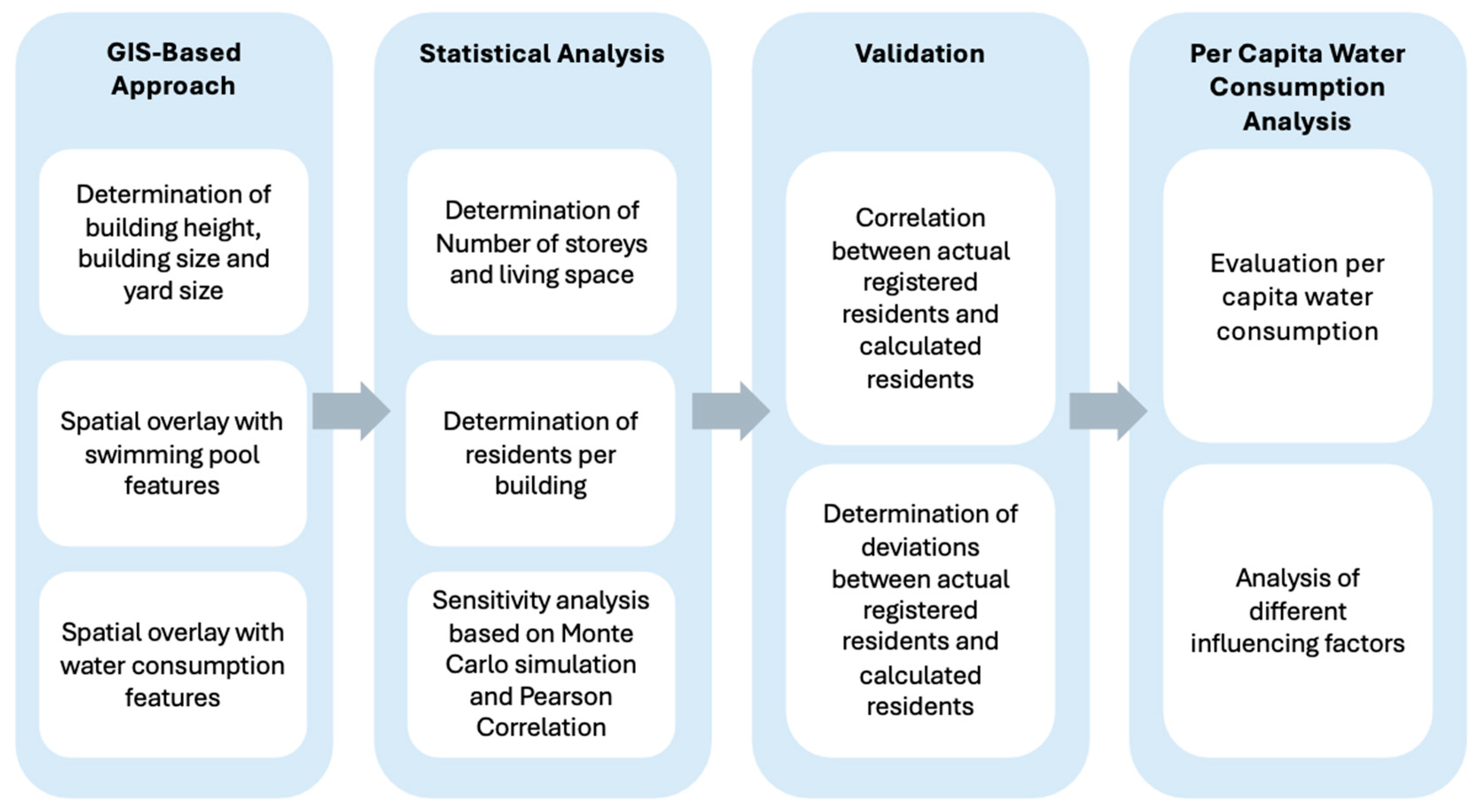
The proposed method can be divided into four steps, as shown in
Figure 1. In step 1, the data are prepared, and the required data are compiled, including cadastral data, DSM, DEM, pool studies, and mean living space. The datasets were then spatially linked within a GIS environment, and building height, building area, and yard size were determined. In the second step, outlier removal was carried out and the residents per building were calculated based on building size, building height, and mean living space. Furthermore, in the second step, a sensitivity analysis of the input parameters was performed using a Monte Carlo simulation and a Pearson correlation. In the third step, the calculated residents per building were compared to the registered residents per building. In the final step, the residential per capita water consumption based on different building types was derived.
The individual steps are described in more detail below.
2.2.1. GIS-Based Approach
The GIS analysis is conducted using ArcGIS or QGIS [
29,
30]. Data preprocessing involves coordinate corrections, attribute standardization, and the transformation of all datasets into a common coordinate system to ensure consistency. Based on cadastral data, DSM, and DEM, key property attributes such as building height, building size, and yard area are determined. To estimate building heights, open-source elevation data, specifically DSM and DEM [
29], are used. The height values are derived by calculating the difference between DSM and DEM. Buildings are then extracted from the cadastral dataset and spatially overlayed with the computed height values.
The yard area is determined by subtracting the building footprint from the total cadastral parcel area. Gaps within the resulting polygons are closed using the Eliminate Polygon Part function. The final yard area is then calculated using the Calculate Geometry function and stored in a new attribute field. Private swimming pools are identified using OpenStreetMap data. All available pools are selected via attribute filtering based on the category “swimming pool” and saved as a vector file.
A spatial relationship is established by linking properties, swimming pools, buildings, and water consumption data through a spatial join. Only clearly assignable data are considered, while water consumption represented by point features located outside property boundaries and properties with multiple consumption point features that cannot be assigned to specific buildings are excluded
The final dataset includes property ID, building type (single-family home or apartment building), pool presence, yard size, building size and height, and water consumption per property. The processed data are then exported and analyzed in R (version 4.3.3).
2.2.2. Statistical Analysis
In R, the data underwent a plausibility check, using the 10th and 90th percentiles, which identified outliers and implausible objects and excluded them from the analysis. Properties without consumption were excluded from further analysis. To determine the number of residents per building, information on mean living space per resident is required. Several literature sources were found on how much living space is available per resident on average in Austria, depending on the building (single-family home or apartment building). According to the literature [
31,
32], the mean living space per resident for a single-family home is 56 m
2 and for an apartment building is 43 m
2.
Furthermore, the mean storey heights (3 m) were estimated based on the literature [
33] and taking into account standard construction methods for ceiling and floor constructions [
34,
35]. This information formed the basis for the calculation of the number of storeys per building, which was determined using the following Equation (1):
Subsequently, the living space of the buildings was calculated and then divided into gross and net building area. As the gross building area also includes non-habitable parts such as wall thicknesses, the building area was adjusted by applying a region-specific reduction factor (0.7), based on literature [
36]. This factor can vary depending on the region. The net living space was calculated using the following formula:
In Austria, single-family homes are often equipped with a gable roof; therefore, the attic was excluded from the living space. The number of residents per building could be calculated by dividing the living space by the mean living space per resident from the literature:
Furthermore, a sensitivity analysis was carried out to estimate the influence of the individual parameters. A Monte Carlo simulation and a Pearson Correlation were used for this purpose. The Monte Carlo simulation required ranges for the input parameters. The range for the storey height was derived by considering different room heights and different ceiling and floor structures. The reduction factor for the net living area was set to a plausible range of 0.65 to 0.75. A distinction was also made between single-family homes (SFH) and apartment buildings (AB). The ranges of the living space per person were estimated based on average living space. A total of 1000 Monte Carlo simulations were carried out with random values for three parameters within the bandwidths. The ranges used in the simulation are shown below.
Storey height (2.75–3.25 m)
Reduction factor for net living area (0.65–0.75)
Living space per person (SFH 50–62 m2 and AB 39–47 m2)
These values are used to estimate the number of residents per building for different combinations. The calculation of the number of storeys and the net living space is calculated using the formulas described above. The relationship between the input parameters and the estimated number of residents is determined using the Pearson Correlation.
2.2.3. Validation
Finally, to evaluate the calculated number of residents per building, the calculated number of residents is compared with the actual registered number of residents per building. Furthermore, it is examined how many buildings can be determined with the exact number of residents and what percentage of buildings can be determined with an error rate of ±1 to ±4 resident. This validation serves to check the plausibility and accuracy of the results.
2.2.4. Per Capita Water Consumption Analysis
The average per capita water consumption is then calculated by dividing the water consumption per building by the number of residents. For Study Site 1, the mean daily water consumption per person is derived from the daily water consumption records. For Study Site 2, the mean daily water consumption is calculated from the annual consumption records. Buildings are categorized into single-family homes and apartment buildings. Single-family homes are further classified based on presence of a swimming pool and yard size (<400 m2, 400–800 m2, >800 m2). To analyze the influence of household size on water consumption, the household size was categorized into one-person households, two-person households, three-person households, and four and more person households.
3. Results and Discussion
This chapter presents the results of the conducted analyses. First, the results from the GIS and R evaluation are presented. This is followed by a detailed analysis of per capita water consumption as a function of the different building types.
3.1. GIS-Based and Statistically Driven Approach
3.1.1. Study Site 1
In Study Site 1, 258 buildings were analyzed, with building heights ranging from 4 to 22 m, determined using GIS. Of the 258 buildings, 89 were single-family homes and 169 were apartment buildings.
Figure 2 illustrates the distribution of registered residents per building, showing that the number of registered residents per building is rather low in single-family homes. There are a few apartment buildings with only two or three residents, which could indicate an error in the classification provided by the water utilities, as it is unlikely that only two or three residents live in an apartment building.
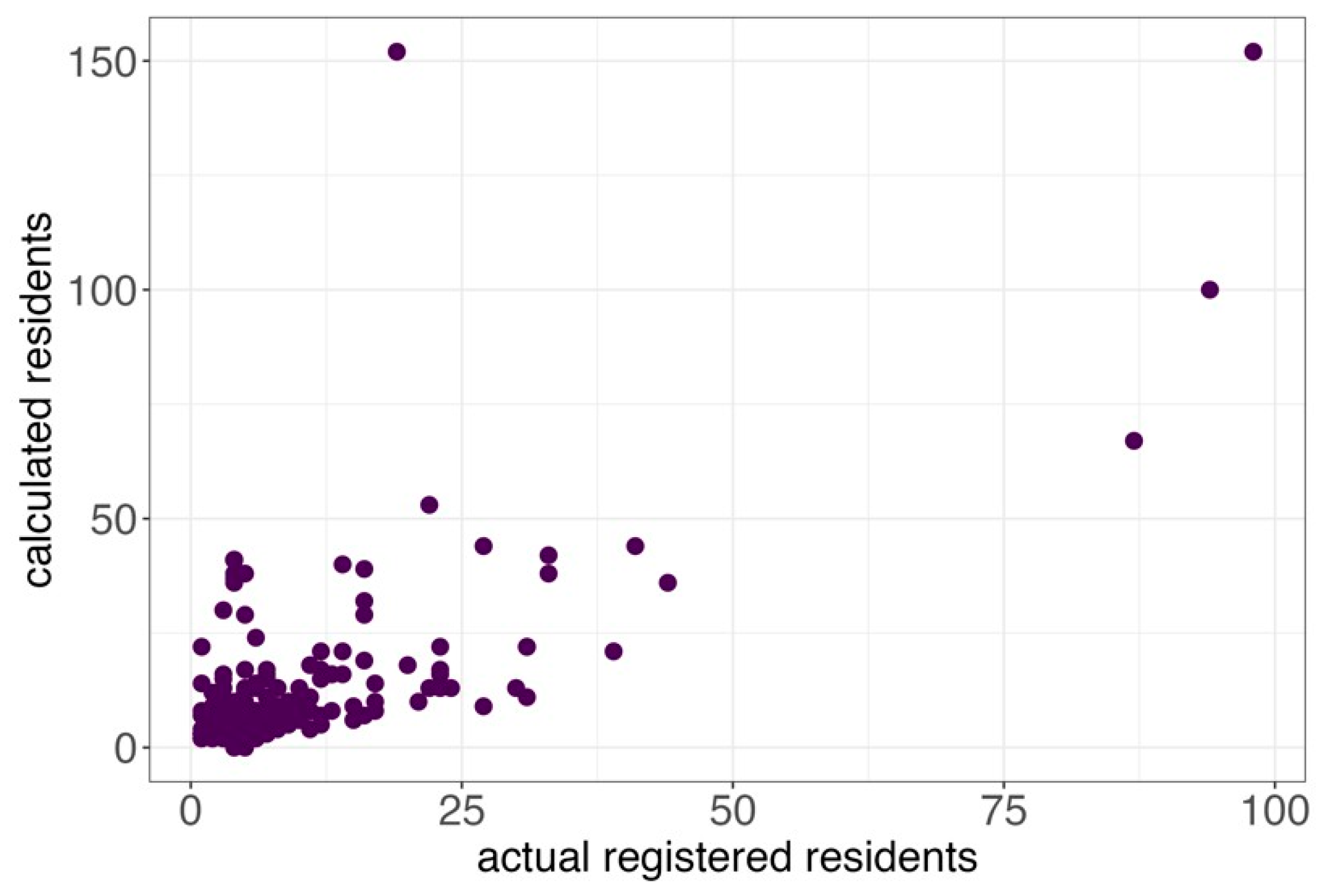
After calculating the number of residents per building according to the methodology described above, the results were compared with the registered number of residents per building.
Figure 3 shows a correlation plot between calculated and registered residents. It shows a slight overestimation of residents, especially for higher numbers of residents. The overestimation could be due to large living spaces in single-family homes, the reduction factor from gross to net living space, or the average living space per person. The reduction factor may not reflect the total living space accurately enough for apartment buildings. In addition, the mean living space could vary in the individual areas and therefore also lead to an overestimation. The Pearson correlation was calculated between the actual and calculated residents. This resulted in a correlation of 0.7, indicating a positive relationship, confirming that the method chosen provides a reliable estimate of the residents and thus a basis for further analysis.
Figure 4 shows a heat map of the calculated versus actual household sizes. It shows whether the previously defined household size classification was adhered to in the calculation. The y-axis represents calculated residents and the x-axis the registered residents, with the color gradient indicating building counts. The results show that the actual one-person households are overestimated, as well as the two- and three-person households.
Figure 5 shows the distribution of calculated and registered residents per building. A slight overestimation of the calculated number of residents can be seen. For apartment buildings, outliers of more than 80 residents per building were cut off for better visualization, with one extreme case of 150 calculated vs. 100 registered residents.
On average, apartment buildings had seven registered residents per building and nine calculated residents, while single-family homes had an average of three residents in both cases.
The median resident number was accurately verified for single-family homes, while for apartment buildings, an approximation of plus 2 persons is already a good result. In addition, we checked for how many buildings the exact number of residents could be determined. The results are shown in
Table 1. The accuracy is good for single-family homes, with the exact number of residents being determined for 19% of all buildings. Allowing a ±1 person bandwidth accuracy increased to 66%, and with ±2 persons, it exceeded over 90%. For apartment buildings, only around 6% were calculated correctly, but with an accuracy of ±4 persons, around 51% of the buildings were calculated correctly.
However, excluding single-person households improves accuracy for single-family homes with 27% exact matches and 75% with a bandwidth of ±1 person, confirming the consistent overestimation of single-person households.
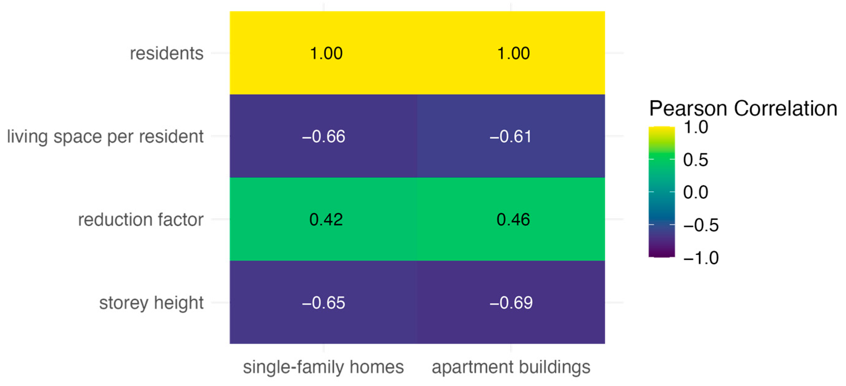
The results of the sensitivity analysis are shown in
Figure 6. The further the colors move towards yellow or dark purple, the more important the parameters are. For single-family homes, living space per resident (−0.66) and storey height (−0.65) are the most important parameters. For apartment buildings, storey height (−0.69) and living space per resident (−0.66) are also significant parameters, and the reduction factor is slightly higher than for single-family homes at 0.46. The results indicate that the adjustment of living space and average storey height has the greatest influence on the calculation of residents. To transfer the method to other areas, the relevant parameters can be adapted to the respective local conditions. This enables flexible application so that the estimates can be optimized while taking regional differences into account.
However, it can be said that the residents could be determined with sufficient accuracy. This method therefore makes it possible to estimate the number of residents per building in the absence of population register data. When applying the method, however, regional factors such as mean living space or storey height must always be adjusted accordingly.
3.1.2. Study Site 2
In total, 29,615 buildings were available for Study Site 2. After the outlier removal (described in
Section 2.2.2) of water consumption, cadastral data, and building heights, 17,131 buildings were found to be suitable for further analysis, including 12,814 single-family homes and 4317 apartment buildings. Yard sizes for single-family homes were categorized as described in
Section 2.2.1. Category 1, less than 400 m
2, contains 2726 properties. Category 2, 400–800 m
2, contains 992 properties and category 3, more than 800 m
2, contains 9096 properties. Additionally, 1818 single-family homes were identified as having a swimming pool.
The number of residents per building was calculated as described in
Section 2.2.2.
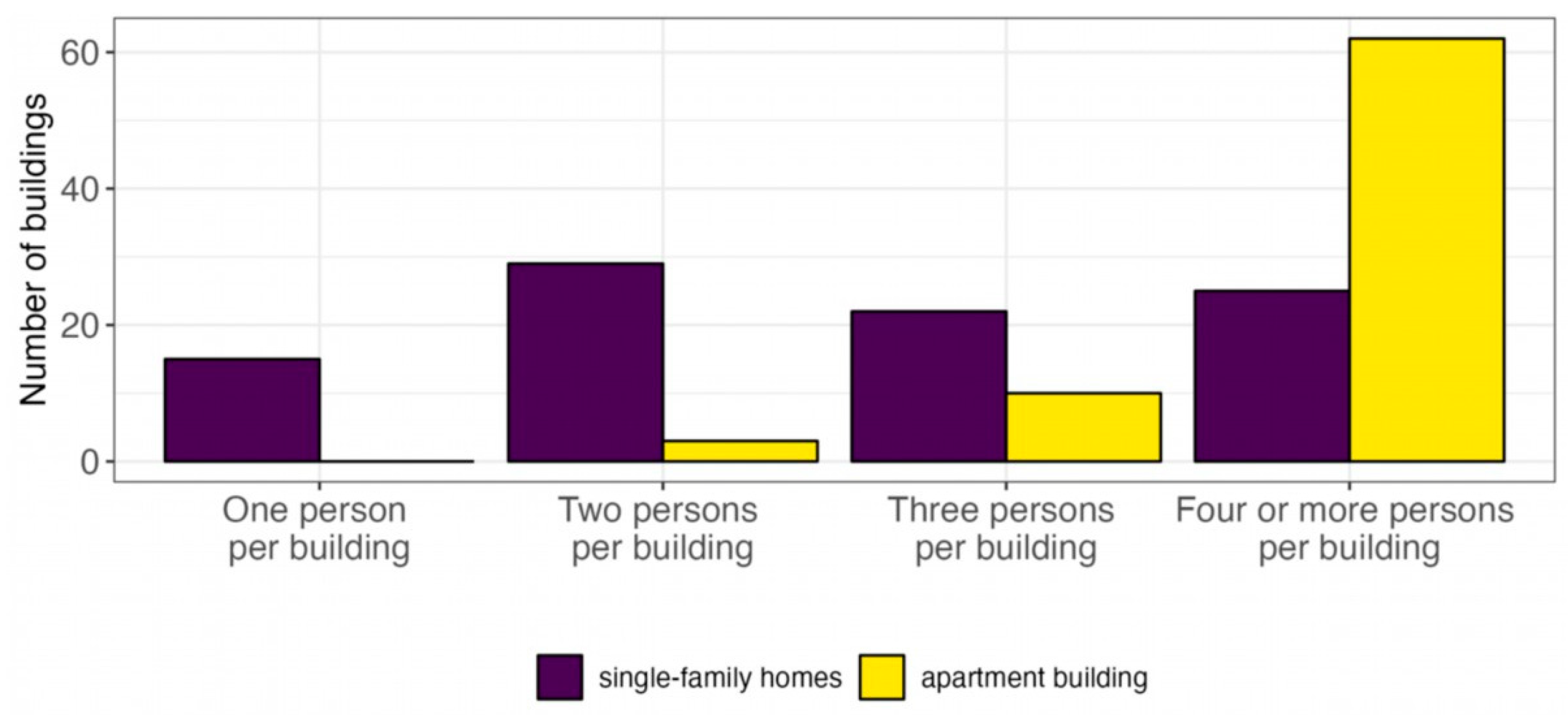
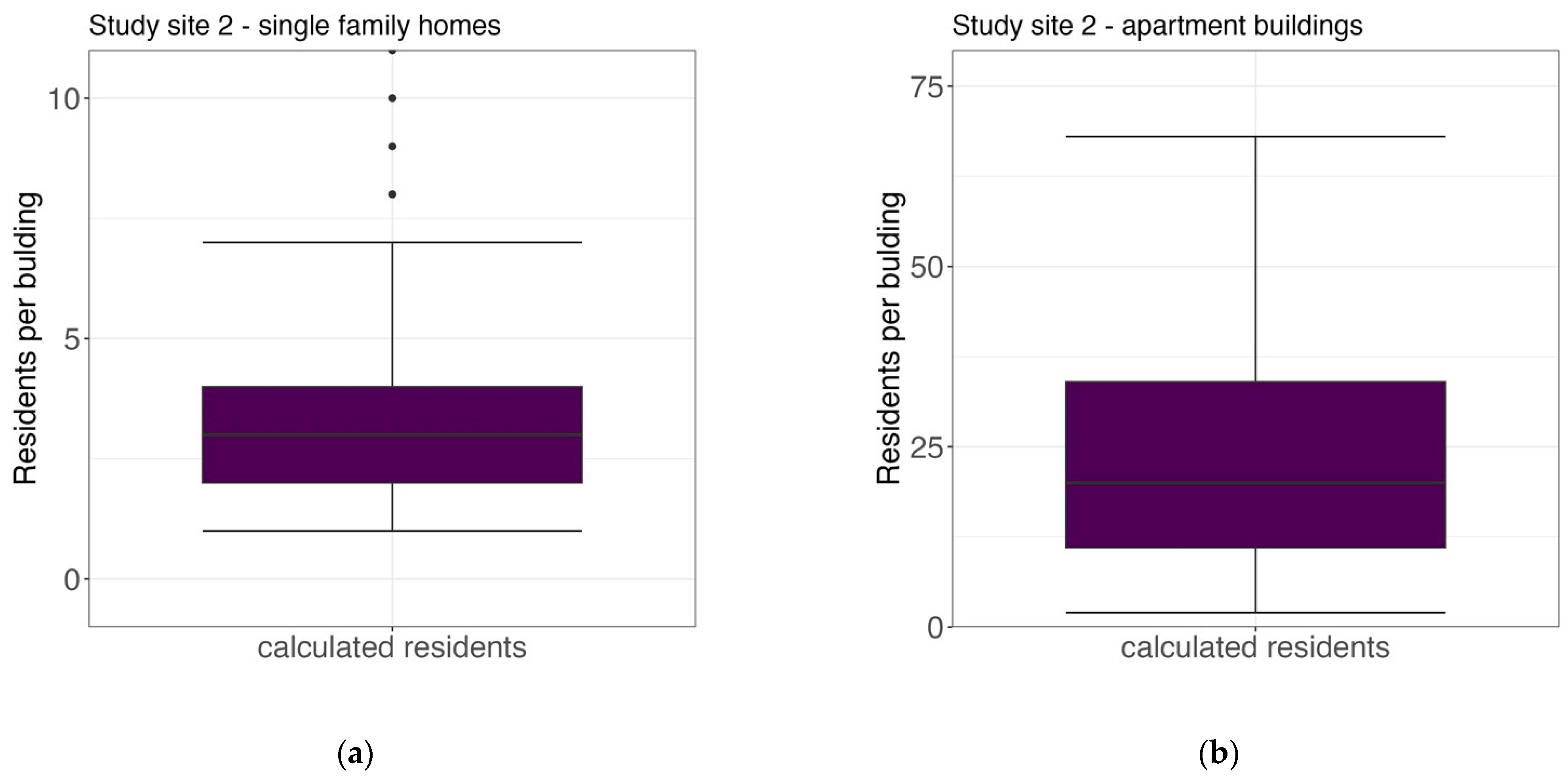
Figure 7 shows the distribution of the number of buildings categorized by occupancy, showing the frequency of buildings with one, two, three, or more residents per building. As mentioned above, the assumption here is also that the two- and three-person apartment buildings have been incorrectly categorized by the water utility, as the size suggests that they are single-family homes.
The average number of residents per single-family homes and apartment buildings was determined next, with the results depicted in
Figure 8. The average number of residents living in single-family homes is three, like in Study Site 1, but there is a big difference in the number of residents living in apartment buildings. At Study Site 2, the average occupancy per apartment building is approximately 22 persons. Given that Study Site 2 is a larger urban area compared to Study Site 1, this higher occupancy rate per building is reasonable.
Based on these evaluations, the per capita water consumption was determined next.
3.2. Per Capita Water Consumption Analysis
This chapter presents the evaluations of the average per capita water consumption. Real historical water consumption was used for this purpose.
Figure 9 shows the per capita water consumption in single-family homes and apartment buildings for both study sites. The results show that, on average, residents of single-family homes consume more water per day than residents of apartment buildings. In Study Site 1, the median daily water consumption per person is around 129 L in single-family homes and around 114 L in apartment buildings. In Study Site 2, the average daily water consumption per person in single-family homes is the same as in Study Site 1 and in apartment building it is around 105 L.
As can be seen from the literature [
14,
15], the increased per capita water consumption in single-family homes could also be related to outdoor water consumption, due to garden irrigation and swimming pools. Furthermore, as shown in the literature [
5,
12,
13], this could also be an indicator of socio-economic differences; residents who live in single-family homes often have a higher income, which, according to various studies, often correlates with higher water consumption. Based on this assumption, the single-family homes were subjected to further analysis, in which the influence of yard size and the presence of a swimming pool on per capita water consumption was investigated.
Figure 10 shows per capita water consumption as a function of household size, showing that single-person households have the highest per capita water consumption, while water consumption per person decreases as household size increases. This can be attributed to activities such as dishwashing and laundry, which are shared by several residents.
Figure 10a represents Study Site 1 and (b) Study Site 2. A comparison of the two diagrams shows a greater bandwidth in Study Site 2, while the median per capita consumption for single-person households is higher in Study Site 1. For larger households, the median values are similar in both study sites.
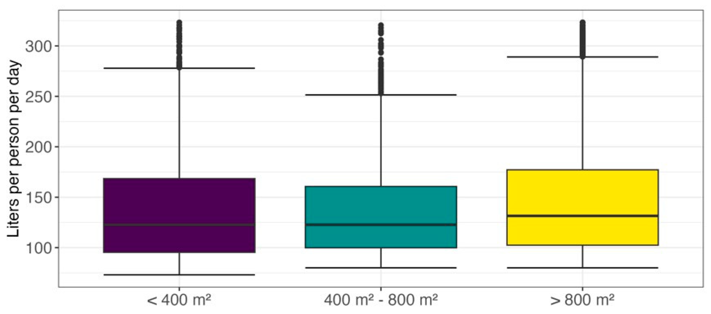
Figure 11 shows the per capita water consumption in single-family homes for different yard sizes. A slightly higher water consumption is observed for larger yards, with median consumption remaining similar to yards under 400 m
2 and those between 400 and 800 m
2.
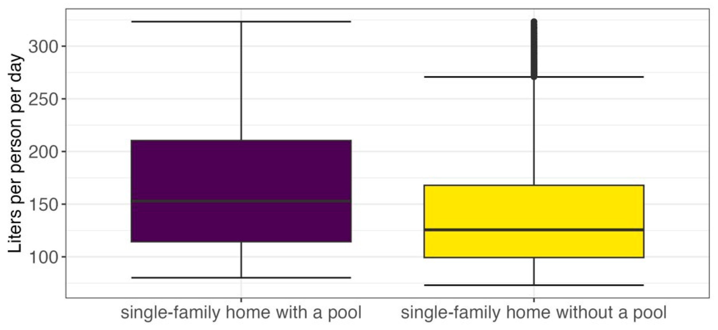
In addition, the impact of swimming pools on per capita water consumption was analyzed, considering only the presence, not the size.
Figure 12 shows that residents in single-family homes with pools have a significantly higher water consumption than those without a pool. This result is also consistent with the literature [
12,
14,
15]. The median daily water consumption per person in a single-family home with a pool is around 153 L per day, while it is around 126 L per day in a single-family home without a pool.
The results above are consistent with the literature, confirming that the proposed method can estimate the number of residents per building with sufficient accuracy to determine average per capita water consumption. This approach allows water utilities to make a rough estimate, even if not all data are fully available. It was also confirmed that single person households have the highest water consumption. In addition, both the size of the yard and the presence of a swimming pool have a significant impact on water consumption. However, other socio-economic factors may also play a role, as shown in the literature. There could be a possible correlation between higher income, age, or education level and single-family homes. However, as no such data are available for this study, this influence cannot be empirically confirmed here.
Nevertheless, the regional sensitivity of the method must be considered, as it relies on site-specific parameters such as average living space, building types, gross-to-net floor area reduction factors, and average floor heights. These assumptions introduce uncertainty, as the approach is, by nature, an estimate rather than a precise measurement.
Another limitation is the variability in data availability, particularly for building heights, sizes, and water consumption, which can affect the accuracy of the estimates. Consequently, the methodology needs to be adapted to regional conditions to ensure its reliability in different geographical settings.
4. Conclusions
Understanding the average per capita water consumption of the supplied population is crucial for water utilities to effectively plan and guide future developments in a sustainable manner. However, to estimate possible influencing factors, such as the type of building or presence of swimming pools on per capita water consumption, knowing the number of residents per building is required. In some regions of Austria, these data are not available to water utilities due to privacy regulations. For this reason, this study developed a GIS-based and statistical approach using open-data and data available at water utilities to determine residents per building. Using this method, the residents could be estimated with sufficient accuracy. A correlation of 0.7 was found between actual and registered residents, with a slight overestimation of the number of residents. This results mainly from using average storey heights and living spaces, as well as a reduction factor, which likely needs to be adjusted when converting the total living space into net living space. This adjustment is necessary because apartment buildings have more communal areas that are not included in the average living space per person. It should also be mentioned that the number of residents reported is only a sample and can change over the course of a year. A limitation of this study is its regional sensitivity, as the method is based on site-specific parameters such as average living size, building types, and gross-net reduction factors, which introduce uncertainties due to its estimation nature. To improve accuracy, a correction factor based on the difference between estimated and registered population figures or a regression adjustment using socio-economic factors and census data could be used. Regional differences could be identified through additional surveys and interviews, e.g., on the average living space per person in the respective service area.
The results of the per capita water consumption analysis show that residents of single-family homes in both study sites use an average of about 130 L per day. In Study Site 1, the average per capita water consumption for residents of apartment buildings is about 114 L per day and in Study Site 2 about 105 L per day. The presence of swimming pools was identified as an important factor. The results show that a resident of a single-family home with a swimming pool consumes about 153 L per day, while a resident in a single-family home without a swimming pool consumes about 126 L per day.
This method offers a good opportunity to make generally valid statements about the average per capita water consumption in the absence of residents per building. An increase in water demand is expected in urban and peri-urban areas of Austria due to population growth. However, this increase in water demand can be influenced by decision-makers due to its dependence on the type of regional development. If many single-family homes with swimming pools continue to be built, these will naturally have a higher water demand than high-density residential buildings. It is also predicted by Statistic Austria [
37] that the number of single-person households will continue to increase. Shown in this study, single-person households have the highest water demand per capita. Underlined by the results of this study, decision-makers can influence future consumption, but it is also not yet known whether climate change and changing factors will lead to a change in the population’s consumption behavior or whether consumption will be regulated by ordinances in the future. Therefore, further research is needed in this area, particularly on changes in probable consumer behavior due to climate change and how this might affect peak demands. Beyond the current application, the method could be extended for predictive simulations of future water demand scenarios. By integrating demographic trends, climate change projections, and urban development patterns, the model could help to estimate future population growth, shifts in settlement patterns, and changes in outdoor water consumption due to climate variability. The inclusion of machine learning techniques or regression-based forecasting could improve the predictive capabilities of the model. However, further validation using historical data and regional adjustments would be necessary to ensure accuracy and reliability across different future scenarios.


