Article

Benefits of an Airborne Electromagnetic Survey of Former Opencast Lignite Mining Areas in Lusatia, Germany

1
Department of Groundwater and Soil Science, Federal Institute for Geosciences and Natural Resources (BGR), 30655 Hannover, Germany
2
Department of Research and Development Centre for Post-Mining Areas, Federal Institute for Geosciences and Natural Resources (BGR), 03048 Cottbus, Germany
*
Author to whom correspondence should be addressed.
Water 2025, 17(7), 1000; https://doi.org/10.3390/w17071000
Submission received: 17 February 2025 / Revised: 25 March 2025 / Accepted: 26 March 2025 / Published: 28 March 2025

Abstract

:
A large contiguous former opencast lignite-mining district is located in Lusatia, Germany, about 100 km south of Berlin. Since this region has been heavily polluted by acid mine drainage from opencast lignite mines, time- and cost-efficient investigation methods are required to obtain comprehensive information on aquifers. In summer 2021, BGR carried out a helicopter-borne electromagnetic (HEM) survey with its helicopter and a RESOLVE system covering an area of about 250 km2. While current surface water levels are derived from in-flight altitude measurements, the spatial resistivity distribution shows indications for the water table in the entire survey area. Apparent resistivities agree very well with water resistivities measured in larger lakes, where the distance to the lakeshores outreaches the system’s footprint. While groundwater sampling requires observation wells, we use HEM results to close the gaps between the sparsely distributed wells. The analysis of groundwater samples shows that groundwater EC correlates with dissolved iron (Fe2+) and sulfate (SO42−) content. HEM resistivities help to approximate groundwater EC, and further Fe2+ and SO42− contents at the observation wells, and to estimate these within the mining area where oxidative pyrite weathering processes dominate other contamination processes.

1. Introduction

Hydrochemical contaminations such as acid mine drainage (AMD) from opencast mines as well as increased susceptibility to soil instabilities pose major challenges for the sustainable rehabilitation and reclamation of post-mining landscapes. In this paper, we focus on groundwater related problems using airborne electromagnetic (AEM) data for a large-scale survey within the Lusatian mining district in Germany. This area (Figure 1) forms the largest contiguous opencast lignite-mining district (814 km2) in the EU and has been mined for around two centuries. Most of the former lignite mines have been closed during the last three decades and a post-mining recultivation is ongoing [1,2,3,4].
In Lusatia, loose Cenozoic sediments (sands, silts, clays, and glacial tills) form several tens of meters of heterogeneous lithological successions in extensive opencast dumps. However, the effects of newly formed depositional structures, spatial heterogeneities, the rising of the water table, and the pore water mineralization of the opencast dumps on groundwater flow and mass transport remain largely unknown in the post-mining areas of Lusatia. In particular, acid mine drainage is a severe problem in the lignite mining area for both post-mining lakes and groundwater [4]. The oxidation of sulfides such as pyrite (e.g., [5,6]), being present in the lignite coal itself as well as in the hosting material, is responsible for causing AMD [7]. Therefore, comprehensive, meaningful, time- and cost-efficient geoscientific methods for the investigation of former opencast lignite mines are required.
The effect of former mining areas on the environment is usually investigated at selected measuring points using boreholes and in situ samples. This means that the most accurate data can be collected at certain points, but can only be conducted there, resulting in spatial data gaps that must be interpolated to obtain a continuous spatial representation [8]. Geophysics can help to close this gap. For example, Gondolfo [9] discusses the determination of water table depth and several papers describe the mapping of ACM distribution using geophysical methods [10,11,12]. Among the geophysical methods applicable on the ground [13], only those that do not require direct ground contact are suitable for airborne surveys [14].
Airborne electromagnetic surveys served and still serve to acquire large baseline datasets in groundwater and soil exploration (e.g., [15,16,17]). AEM results combined with data and models from external sources (e.g., boreholes, groundwater samples, ground-based geophysics, geological models) enable the derivation of spatial estimates, which then may serve as the baseline data for advanced (hydro-)geological modeling (e.g., [18,19,20,21]). While AEM has already been frequently used in groundwater surveys (e.g., [22,23]), only little is known about airborne geophysical investigations of (former) opencast lignite mining areas [24,25]. Most of the airborne (and spaceborne) surveys reported in the literature applied remote sensing technologies to investigate abandoned opencast mines and their impact on the environment (e.g., [7,26,27]).
Due to there only being local (in situ data) or non-existent (soil geophysical data) information on groundwater contamination caused by mining, the Federal Institute for Geosciences and Natural Resources (BGR) conducted an airborne geophysical survey in a former opencast lignite mining region near the towns of Cottbus and Senftenberg in Lusatia, Germany, in summer 2021 [28]. The main objective of BGR’s airborne survey was to outline the benefits of an airborne geophysical investigation for the characterization of opencast dumps in terms of their (hydro-)geological setting. The investigation focuses on revealing information on aquifers and, in particular, on their depth and mineralization by AMD down to a depth of about 100 m below ground level.

2. Materials and Methods

2.1. Geology and Hydrogeology of the Survey Area

The survey area is located in the western part of the Lusatian lignite mining area between the Elster River lowland in the south and the terminal moraine and outwash plains of the Lower Lusatian border wall in the northeast (Figure 2).
During the Palaeogene and Neogene, Lusatia lay on the southern edge of the Palaeo-Northern Sea. As a result, the area was particularly exposed to the influences of rising and falling sea levels. The frequent spatial and temporal changes in the marine, brackish, and terrestrial depositional areas can be attributed to global and climatically induced sea level fluctuations [34]. This led to the formation of five lignite seam horizons in the area of the large coastal bogs [35]. Locally, the uplift and subsidence of the Mesozoic–Paleozoic basement occurred in the geological subsurface, which is associated with tectonic activity during the Neogene [36]. The Pleistocene deposits are up to 150 m thick and consist mainly of glacial, interglacial, fluvial, and lacustrine sediments (sand, silt, clay). The repeated advance of the inland ice from northern and northeastern Europe into the Lusatia region led to complicated bedding conditions and subglacial valleys that cut into the Cenozoic and Mesozoic layers [36].
As a result of the commercial open pit mining of the second Miocene lignite seam since the 1920s, the original geological layer sequence above the lignite seam was removed to depths of about 80 m above sea level (asl) and relocated on overburden dumps. The surveyed post-mining landscape is part of the LMBV (Lusatian and Central German Mining Administration Company) remediation area. The extensive remediation areas of lignite mining in Lusatia consist of former opencast dumps with anthropogenically altered deposition conditions and the adjacent post-mining lakes.
The shallow aquifers of the investigation area drain their water to the tributaries of the Schwarze Elster, which is a second-order stream of the Elbe Basin with a total length of 179 km. In the central region of the investigation area, the surface water system consists of 18 post-mining lakes, which are connected by 9 km of constructed water channels forming the so-called “Kleine Restlochkette” (small chain of post-mining lakes). The surface water quality in the central region is heavily impacted by the AMD leachate. The groundwater declines towards the west, except in the northeast of the survey area at higher elevations [37], where no lignite mining has taken place (Figure 2). There, higher lake water levels occur and perched aquifers are to be expected.

2.2. Airborne Geophysical Survey
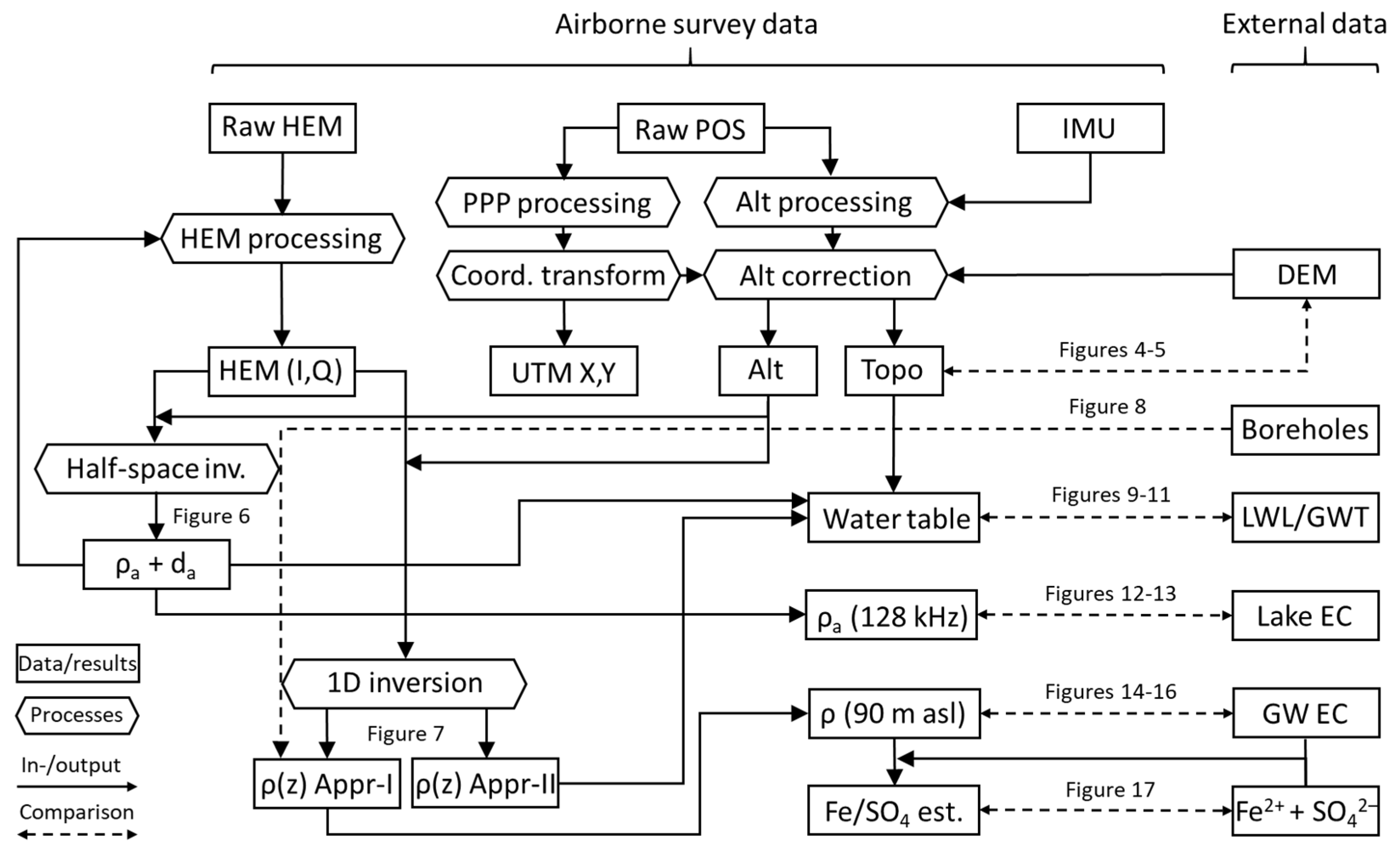
In July 2021, BGR conducted a one-week airborne survey (1736 line km, nominal separation of the NW–SE flight lines: 250 m) over an area of 250 km2 between Finsterwalde and Lauchhammer about 50 km southwest of the city of Cottbus in eastern Germany ([28], Figure 2). The airborne geophysical system used consists of a Sikorsky S-76B helicopter, three geophysical (electromagnetic, magnetic, and gamma-ray spectrometric), navigation, and positioning (incl. inertial measurement unit) systems, a data acquisition system, and a base station recording diurnal variations. The helicopter-borne electromagnetic (HEM) system (RESOLVE) is operated at six frequencies ranging from 0.4 kHz to 128 kHz with onboard calibration facilities. The transmitter and receiver coils are oriented in a horizontal–coplanar (5 × HCP) or vertical–coaxial (1 × VCX) position. The maximum investigation depth generally depends on the electrical conductivity of the surface water, the groundwater, and the sediments/rocks in the subsurface. Both the penetration depth [38] and the footprint [39] increase with decreasing system frequency and conductivity of the earth. On average, a depth of investigation of 50–150 m and a footprint of 100–300 m (belonging to the highest to lowest frequency of the RESOLVE system and a mean sensor altitude of about 60 m) can be expected [40].

2.3. Airborne Data

The general airborne data processing is described in detail in [28,40]. Here, we focus on position and electromagnetic data. All raw and processed datasets as well as various products (maps, vertical sections) are publicly available via BGR Geoportal. The flow chart in Figure 3 shows the various processing steps, their interaction, and the comparison with external reference data described below.

2.3.1. Position Data Processing

Position data processing includes checking and, if necessary, correcting the position and distance data measured (GPS data of the helicopter and the flying probe (bird) as well as the distance-to-ground measurements with a laser altimeter). For the post-processing of raw data delivered by the GNSS (Global Navigation Satellite System), we use the Precise Point Positioning (PPP) web service of the Geological Survey of Canada (Natural Resources Canada). This post-processing provides a significant improvement for the position data, especially for the critical vertical component. The bird attitude is corrected with the help of an inertial measurement unit (IMU) integrated into the GNSS. We derive the terrain elevation (Topo) from the difference between the GPS elevation and the laser altitude of the bird. As the tree canopy can affect the laser data, a digital elevation model (DEM) is used to check and correct the laser data [28].

2.3.2. HEM Data Processing

The processing of the HEM data, in-phase (I) and quadrature (Q), aims to determine the electrical conductivities (or their reciprocal values, the electrical resistivities) of the earth’s subsurface. The data processing also includes the identification and correction of man-made effects (cultural noise), which are not caused by the (hydro-)geological subsurface, e.g., lightning, interference with power lines or metallic installations (cables, fences, rails). System-related causes, such as incorrect calibration, thermal electronic drift, data noise, and motion-induced effects, can also affect the HEM data [41]. Weak local effects can usually be reduced by suitable filters (non-linear and low-pass filters), but larger effects have to be marked, and the corresponding data sections are removed. Smaller data gaps can often be filled by suitable interpolation. In order to reduce the system-related effects, however, plausibility checks, drift correction, and line leveling are necessary. Transformed HEM data derived from homogeneous half-space models [42] are used for this purpose. In contrast to the HEM data (I and Q), the half-space parameters, apparent resistivity (ρa), and apparent depth (da), are only slightly dependent on variations of the sensor altitude (above ground) and can therefore be used much better for data quality control and correction [22].

2.3.3. HEM Data Inversion

Homogeneous (single-frequency inversion) and layered (multi-frequency inversion) half-space models are used to derive spatial resistivity distributions. At each frequency of the HEM system, the homogeneous half-space inversion provides an apparent resistivity (ρa) for the half-space and an apparent distance from the bird to the top of the half-space. The difference in the apparent distance to the measured bird altitude, the apparent depth (da), indicates an increase or decrease in resistivity with depth (within frequency-dependent depth ranges). This value is negative for a more conductive cover and positive for a more resistive cover with respect to the substratum. In the latter case, da tends to approximate the thickness of the resistive cover layer, provided the corresponding penetration depths are much larger. A measure for the mean penetration depth, the centroid depth (z*), is derived from ρa and da [42].
The multi-layer (1D) inversion applies a Levenberg–Marquardt procedure in combination with general matrix inversion that is able to use both few and many (resistivity, thickness) model layers [43]. Layer interfaces and resistivities are best determined for a few-layer inversion (all model parameters are free) if the subsurface also consists of a few dominant layers with clear resistivity contrasts. Otherwise, the inversion result is often strongly dependent on the starting model used and layer resistivities and thicknesses may jump from model to model along a survey line [43,44]. A smooth inversion (only the resistivities and the cover layer thickness are free) can better represent gradual transitions in resistivities and complicated structures are easier to recognize.
The starting models for the 1D inversion are derived from apparent resistivity vs. centroid depth sounding curves. The layer thicknesses increase continuously in a range determined by the centroid depths of the highest (zh) and lowest (zl) frequency. The standard approach I subdivides the area above zh using the apparent depth of the highest frequency, whereby the minimum layer thickness is 0.5 m. The resistivity of the cover layer is either set to a high value for a positive apparent depth or extrapolated from the sounding curve [40]. Alternatively, the boundaries zh and zl can be shifted upwards or downwards depending on local conditions, e.g., to reveal near-surface resistivity structures. In approach II, the depth range of the starting model layers with increasing thickness begins close to the surface, i.e., the shallow model region, including the cover layer contains more layers than before.

2.4. External Material

A multitude of datasets from public and closed sources has been used to evaluate and interpret the HEM results (Table 1). LMBV has provided most of the sample data. An excerpt used for the comparison with HEM results is listed in Appendix A.

2.5. Interpretation of HEM Data

2.5.1. Water Table Estimation

Assuming that the resistivity in the unsaturated (vadose) zone is usually higher compared to the saturated zone [47], a water table should be indicated by a resistivity decrease with depths. This expected resistivity decrease should be observable in both homogeneous half-space and multi-layer inversion models. However, it has to be noted that low resistivities can also occur above the water table, e.g., caused by increased soil moisture or clayey layers. We focus on the elevation of the water table, because this surface (in m asl) is presumably smoother than the corresponding depth of the water table (in m below ground level) and therefore less prone to artifacts caused by gridding or smoothing filters.
First, we try to estimate the water table directly from the resistivity models. A simple and fast way to do this is to use the apparent depth da, provided that the corresponding penetration depth lies significantly below the water table. For shallow water tables, da at the highest frequency is suitable. Deeper water tables, however, also require da values at the other frequencies (e.g., dam = maximum of da). Small or negative apparent depths often indicate surface water. We therefore set negative da values to zero, i.e., the terrain elevation derived from the flight data (Figure 4) is used to approximate the water level there. Another option for the water table estimation is to use the cover layer thickness of the 1D inversion models, which also use da at the highest frequency as a starting parameter.
For water tables occurring below the cover layer, approaches that are more sophisticated are necessary to reveal the appropriate resistivity increase, which should be strong in a few-layer inversion and weaker in a smooth inversion. However, the layer boundaries of an inversion with few layers often do not sufficiently coincide with resistivity interfaces, especially if the number of model layers differs from the real (geological/hydrogeological) layering. A smooth inversion, on the other hand, is less prone to this problem, but sharp resistivity boundaries tend to appear smooth. In order to reveal the freshwater–saltwater interface from smooth HEM inversion models in Zeeland (NL), Siemon et al. [40] developed a steepest gradient approach, which we apply here to derive the water table in the entire survey area. This approach consists of three steps: (1) A search of the steepest gradients in all 1D HEM inversion models. (2) An evaluation (selection, smoothing) of the corresponding depth (elevation) of these gradients within the entire survey area. (3) A comparison of the airborne results with water level/table data measured at lakes and in boreholes. Since this approach approximates a spline function to resistivity–depth values of the smooth inversion models below a (sometimes thick) cover layer, shallow boundaries affecting the subsurface resistivity (e.g., water table) may be hard to resolve using the standard starting model (approach I). Therefore, we also apply approach II, which provides several thin model layers close to the surface and thus extends the depth range of the spline function upwards.
A water table should be indicated by the steepest negative resistivity–depth gradient. The corresponding depths (SG) and elevations (SGE) are first selected with respect to an appropriate range of the water table within the current survey area (e.g., known from measurements or literature); in this instance, this is an SG less than 60 m depth and an SGE above 80 m asl. The uppermost SGE focuses on the shallowest water table. However, if there are several aquifers, the automatic evaluation is often unable to distinguish between the low-lying regional and higher-lying local (perched) aquifers. For this reason, the automatic evaluation is not only limited downwards (to 80 m asl) but also upwards (to 135 m asl). A coarse grid (CG, 1000 m cell size) is created to check the SGE values with respect to outliers. Only those values where the deviation of SGE and CG is less than 10 m are used. SGE values with higher deviations are erased and—if existent—replaced by a deeper SG (second steepest negative gradients) if the corresponding SGE lie within the 10 m distance to the CG. Finally, coarse gridding is applied again, followed by resampling along the flight lines or at any other location (e.g., water wells).
The SG approach is not applicable to lake areas because the water levels equal the lake surfaces. Therefore, we replace the SGE values beforehand by the terrain elevation (Topo) derived from the airborne data for the lake areas. The areas of the lakes are estimated from thresholds for the half-space parameters at the highest frequency (apparent resistivities ρa < 30 Ωm and apparent depths da ≤ 0 m), but only for elevations below the highest lake level (Topo < 130 m asl).

2.5.2. Water Quality Estimation

The groundwater in the mining area is heavily polluted by pyrite weathering. This should also be seen in the HEM results due to an increase in the electrical conductivity (EC). Therefore, it is first examined whether the EC values in the lakes correlate with near-surface resistivities derived from HEM. Apart from the transformation of EC values into resistivity values, no further conversions are required. However, the influence of the lake size and the location of the sampling points on the HEM results must be examined.
While surface water contamination can easily be sampled in situ at the surface, observation wells are required for groundwater sampling. The first task is to estimate the formation factor F (Equation (1)), which is carried out through using a simplified Archie Equation [48] to discover the ratio of bulk resistivity ρb to water resistivity ρw
F = ρbw ≈ ρ∙EC/10,000.
The water resistivity can be derived from EC values as before, but the bulk resistivity must be estimated using HEM resistivities ρ, which are influenced by both groundwater mineralization and lithology. Since the filter sections in the wells are generally located in sandy sediments, a formation factor typical for sand can be expected there. However, nearby layers of clay, silt or lignite can influence the HEM data. This effect must be checked. If the HEM resistivities correlate with the resistivities of the groundwater at the observation wells, this result could be transferred to the entire survey area, but only for the sand-dominated areas. The further estimation of certain groundwater mineralization is only possible if the EC values in the groundwater are characterized by a specific element or element pair, such as the salt content in seawater. Here, we focus on iron (Fe2+) and sulfate (SO42−) content.

3. Results

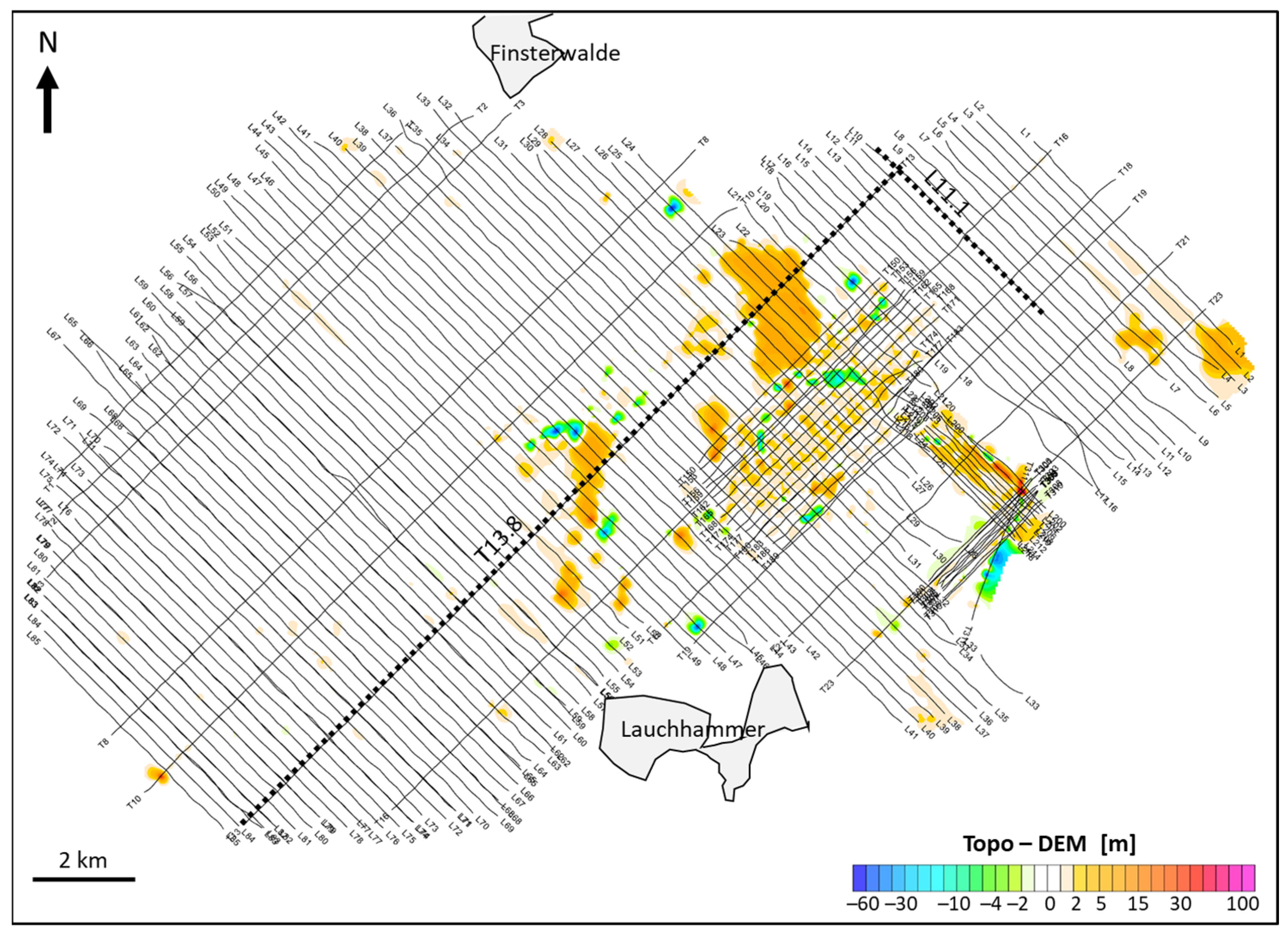
3.1. Terrain Elevation

The current terrain elevation (Topo) derived from flight data was checked and corrected in places using a DEM (DGM25, [45]), particularly outside the mining areas, where trees and other obstacles on the ground can affect the measured data. Inside, however, the DEM used was often unable to correctly map the actual elevation of the changing landscape (Figure 4). The differences between the resulting Topo and DEM values are shown in Figure 5. They are generally very small and only prominent in areas with recent surface elevation changes (e.g., lake water levels, dumps, pits, and slopes).

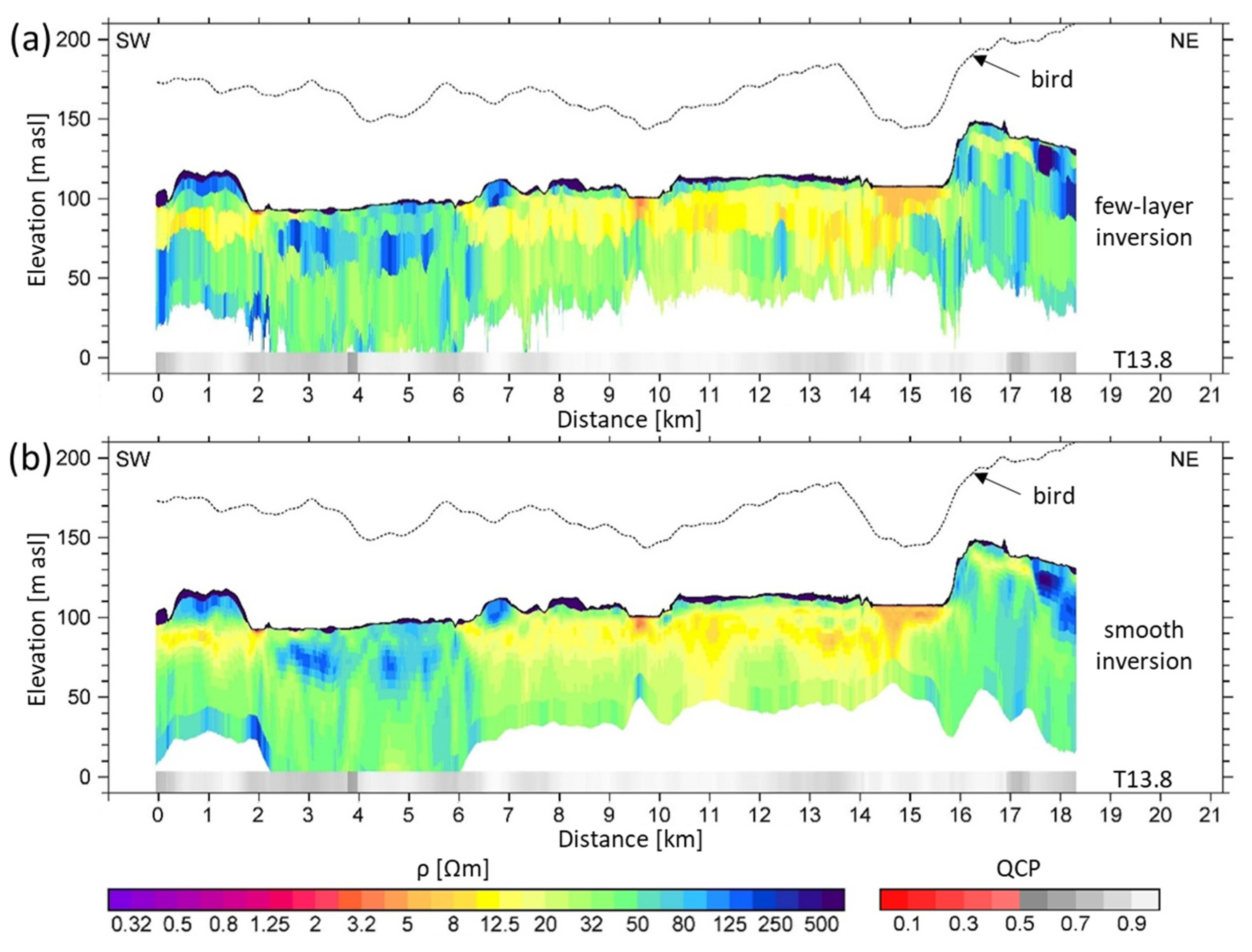
3.2. General HEM Results

The main aim of the electromagnetic survey is to obtain information about the regional groundwater distribution. The focus is set on the current water table and the mineralization of the groundwater as well as the identification of aquifers and aquitards. The HEM results are displayed as colored maps (50 m grid cell size) showing the apparent resistivities at each frequency and the resistivities derived from the 1D inversion models with 20 layers at selected elevations. The inversion models are also displayed as cross-sections consisting of colored resistivity columns stitched together along flight lines with respect to Topo.
Figure 6 provides a first overview of the conductivity distribution in the survey area showing maps of apparent resistivities (half-space resistivities) at all frequencies. As the corresponding centroid depths increase with decreasing frequency (f = 128–0.4 kHz) and increasing resistivity, the maps display the prominent apparent resistivity structures at increasing depths. Higher apparent resistivities occur in predominantly sandy areas with weakly mineralized groundwater (blue colors, ρa ≥ 60 Ωm) and lower values are typical for clay sediments or higher mineralized groundwater (yellow to green colors 10 Ωm < ρa < 60 Ωm) [15]. The lowest values (orange colors, ρa ≤ 10 Ωm) are mostly observed in post-mining lakes with usually significantly increased mineralization.
Generally, we perform both an inversion with few layers and a smooth inversion of the HEM data with starting models consisting of 6 and 20 layers, respectively. As an example, Figure 7 shows the 1D inversion results along an approximately 18 km long SW–NE tie line (T13.8, see Figure 5 for location) that crosses the largest post-mining lake in the survey area (Bergheider See) at 14–16 km on the profile. The color-coded models are shown in relation to the terrain elevation (Figure 4). Both inversion settings lead to similar results. The lowest resistivities occur at about 70–110 m asl in the south-western and central parts of the profile, i.e., in the abandoned mining area. The vertical shapes of the lakes, especially those of Bergheider See, are recognizable best in the smooth version.
Outside the mining area, especially at higher altitudes (e.g., at 16–18 km on T13.8), we do not expect groundwater contamination from mining. Therefore, a section (about 4 km) of a flight line (L11.1) over a small hill is considered here (Figure 8) to show the influence of the lithology on the calculated resistivity. The drilled lithology derived from nearby boreholes (≤50 m distance) is drawn in the resistivity cross-section. In most cases, the conductive areas correlate with silt, clay, and lignite, and the resistive areas with sand and gravel. While layers with increased resistivities bound the shallow conductors, the deeper conductors do not appear to be bounded by depth due to the limited depth of the investigation of the HEM system. On the other hand, the drilled silt, clay, and lignite layers do not appear as continuous layers near the survey line. This indicates—at least in places—a complex lithology in the survey area.

3.3. Special HEM Results
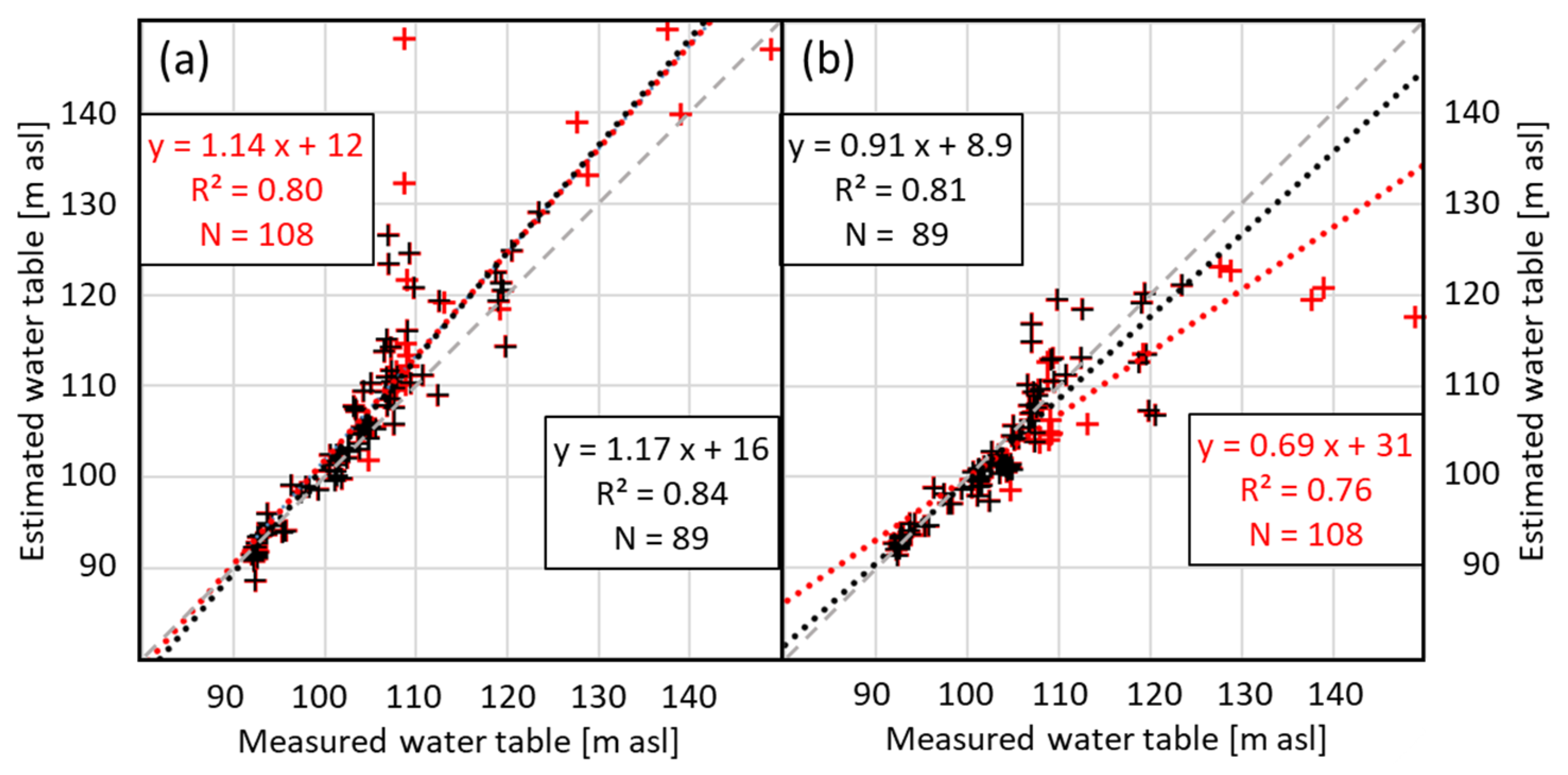
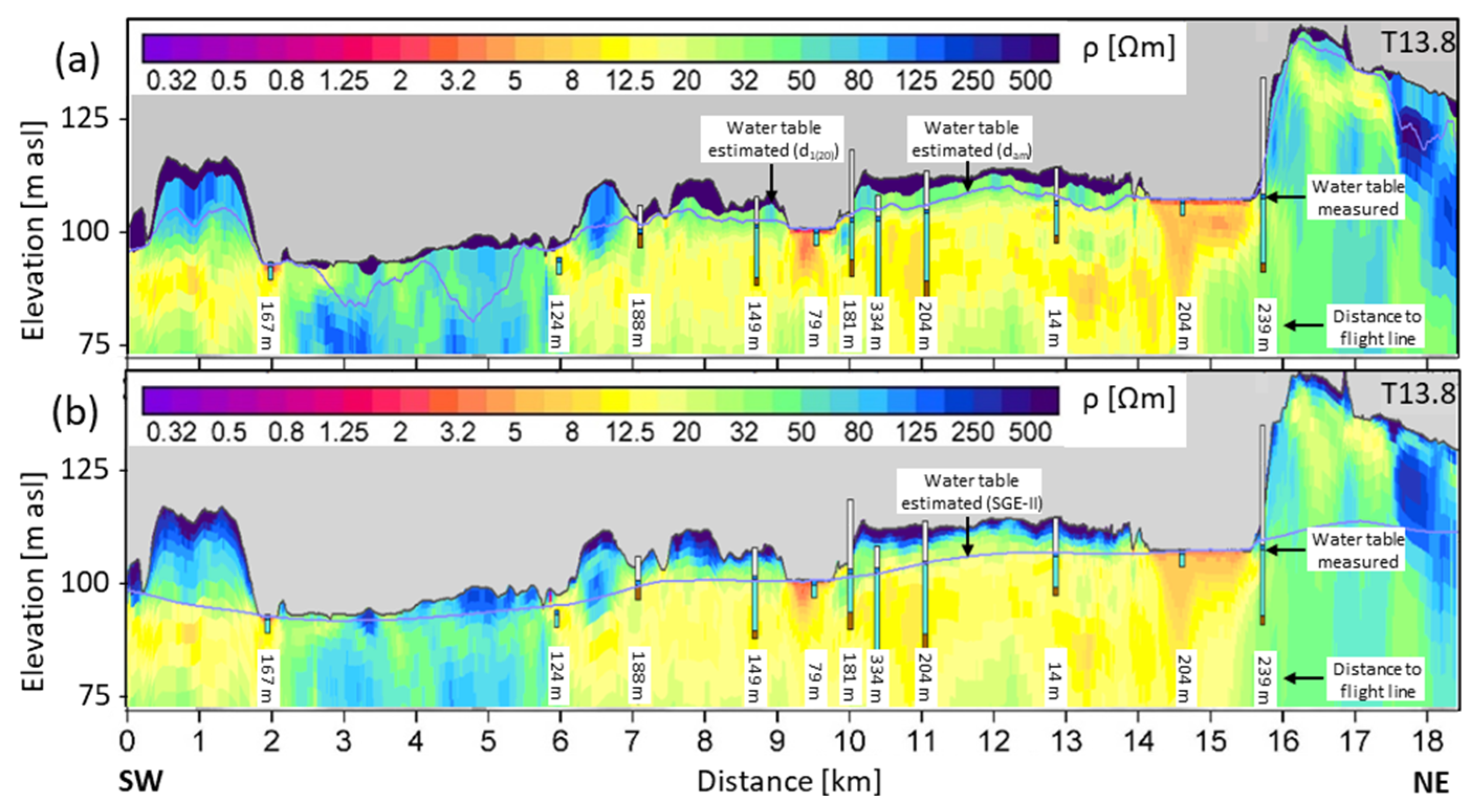
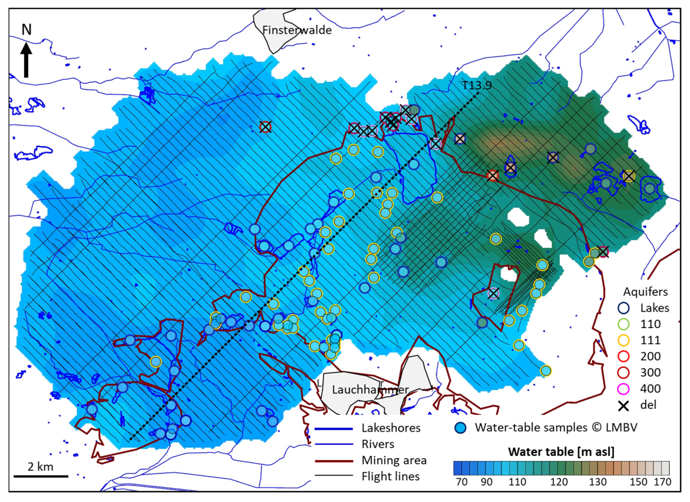
3.3.1. Water Table

The water table in sandy sediments normally varies little and follows the ground surface slightly. In hilly terrain, however, locally varying water tables can occur and a large-scale recording of the water table would require numerous sampling points. Since these sampling points are sparsely distributed within the survey area, particularly outside the mining area, we try to derive the water table from HEM.
First, we estimate the water table directly from the resistivity models. Table 2 shows the mean values (Δ) and the standard deviations (σ) of the elevation differences in the estimated water tables derived from apparent depths da (homogeneous half-space inversion) and cover layer thicknesses d1 (multi-layer inversion) with respect to the measured water levels of the lakes and water tables in the wells (and total). Elevations are derived from da (at 128 kHz), dam (the maximum da at all frequencies), and d1 (cover layer thickness of 6 and 20 layer resistivity models). Most of the water tables recorded at the location of the boreholes belong to the main regional aquifer, but some originate from upper aquifers, especially in the eastern survey area where the terrain elevation is high (Figure 4) and confining layers (clay/silt/lignite) are present (Figure 8). Table 2 also contains the statistical parameters, excluding those 19 samples belonging to perched aquifers (_sel) or lake levels ≥125 m asl. All estimated water tables are too high on average and show a wide variation. The best values can be derived from the elevations of the maximum of the apparent depth values (Figure 9a, total ∆dam_sel = 1.8 ± 3.9 m).
The results listed in Table 2 show that the methods relating directly to the cover layer in the resistivity models do not provide satisfactory results, with the exception of dam. We now apply the steepest gradient method to derive the water table from all of the 1D inversion models. Compared to the measured water table (Table A1 and Table A2), approach I (with partially thick overburden) provides overestimated thicknesses of the vadose zone, i.e., the water tables are below the measured values (Table 3, total ∆SGE-I = −5.5 ± 5.2 m), even with a focus on the selected samples. The statistical results of approach II are shown in Figure 9b. The mean deviation is now significantly lower (∆SGE-II = −1.8 ± 5.0 m), but the slope of the linear regression is not steep enough. The shallow slopes are caused by measured water tables belonging to higher lying aquifers and lakes, which both approaches try to ignore. Focusing on the previously selected samples further reduces the deviation (∆SGE-II_sel = −0.7 ± 2.2 m) and increases both the slope and the R2 value in Figure 9b (black).
Table 3 also shows the differences between the terrain elevations derived from the airborne data (Figure 4) and the surface elevations of the boreholes. Note that some of the high water table deviations listed in Table 2 and Table 3 could also be due to the differences between the terrain and surface elevations (total ∆Topo-SE_sel = 0.7 ± 2.2 m).
Figure 10 shows an example of a vertical section (T13.8), in which the estimated water table (purple line) derived from the HEM models is displayed in comparison with measured values (blue section in colored columns). While the calculated water table based on the cover layer depth of the standard smooth inversion (d1(20), bottom of dark blue cover layer) is generally too high, the values derived from the maximum apparent depth (dam) are often close to the measured values, except for some resistive areas (Figure 10a). The best results are achieved with approach II (SGE-II, Figure 10b).
Figure 11 displays an elevation map of the estimated water table belonging to approach II (Figure 10b) together with the locations of the water samples (wells and lakes), aquifer code, and elevation of the measured water table/level. Black crosses indicate the deselected samples. Similar to [37], the water table mostly falls in a westerly direction, except in the northeast of the survey area. This map also demonstrates that there are only a few measuring points outside the mining area (in particular, there are almost no samples available in the north-west), while there are many inside.

3.3.2. Lake Water EC

Figure 1c,d shows two examples of post-mining lakes in the study area that appear to be contaminated due to their color and presumably also due to their water EC values. The question is now whether the HEM results can reflect the water EC values. These lakes can also be used to check the results of the HEM analysis in comparison with water samples.
In order to check the calibration of the HEM system at the highest frequency, we compare the apparent resistivities in Figure 12 with the EC values of lake water samples provided by LMBV [46] and check the apparent depth values, which should be close to zero (or negative for shallow lakes) in such a case.
The apparent resistivities at 128 kHz (ρa) vary from lake to lake. While most of the lakes within the mining area have lower ρa-values (3–5 Ωm, orange to red colors on the map), the ρa-values at most of the other lakes are quite normal (>10 Ωm, yellow to green colors)—except the lake at the eastern corner of the survey area. These apparent resistivities fit very well with the water resistivities (ρw) in the lakes (converted from measured water EC values: ρw [Ωm] = 10,000/EC [µS/cm], Table A3) as long as the widths of the lakes exceed 200 m so that the distance to the lakeshores outreaches the footprint of the HEM system at the highest frequency (Figure 13). The corresponding apparent depths (da) at the lakes are small, on average being Δda = −0.1 ± 1.1 m, i.e., close to the expected value (≤0 m).

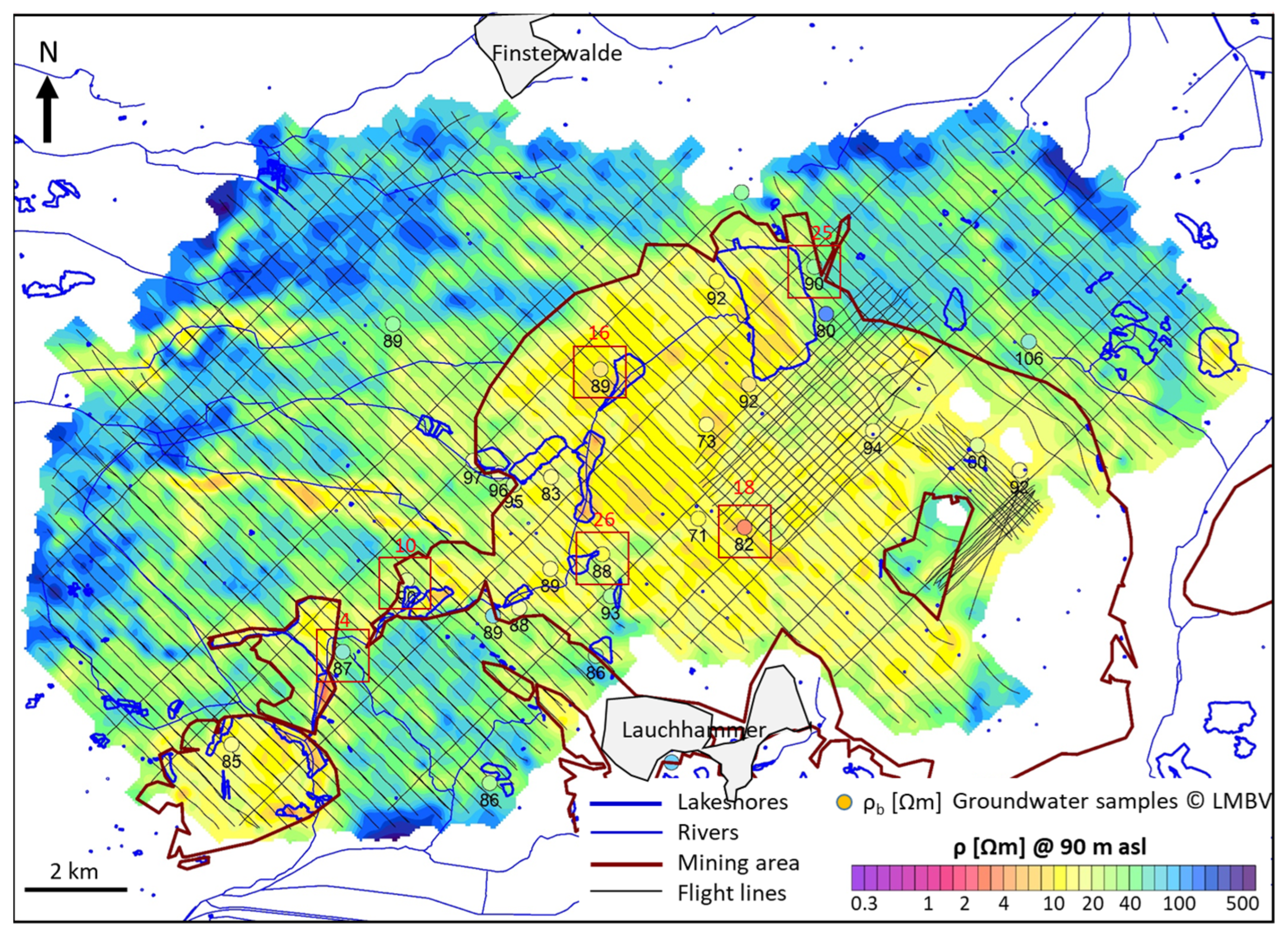
3.3.3. Groundwater EC

As the observation wells are sparsely distributed in the survey area, the question arises whether HEM results can help to close the gaps. Figure 14 shows the resistivity distribution at 90 m asl, derived from 1D inversion models with 20 layers including a cover layer (cf. Figure 7b). The majority of the well screens (in most cases 2 m thick) in the observation wells are located in a sandy aquifer near this elevation. The resistivities ρ at 90 m asl are plotted against the resistivity ρw of the groundwater samples (Table A4) in Figure 15, where a linear relationship can be observed if the two extreme values are ignored. The slope, which should roughly correspond to the formation factor F, is below the expected value of F = 4 for sand.
Figure 14. Resistivity ρ at 90 m asl (grid) vs. bulk resistivity ρb derived from groundwater samples (dots [46]). The mean well screen depth (m asl) is shown below the borehole dots. Red squares indicate the location of the observation wells (red numbers) shown in Figure 16. Rivers [31], lakeshores [32], mining areas [33], and flight lines are marked.
Water 17 01000 g014
Figure 15. Resistivities ρb at 90 m asl vs. groundwater resistivities ρw [46]. Dotted lines indicate the best-fit lines for datasets with (red) and without (black) extreme values; the dashed line indicates the 4:1 line.
Water 17 01000 g015
Figure 16. Resistivity cross-sections (exaggeration ≈ 13) near selected groundwater observation wells (LMBV [46]). The electrical conductivity of the sampled groundwater (EC) and the derived bulk resistivity (ρb) using a formation factor of F = 4 are indicated at the well screen position (arrowheads) on the borehole column (lithological profile). Above ρb, the corresponding HEM resistivity value (ρ) is shown. Δ indicates the distance of the well to the next flight line.
Water 17 01000 g016
However, when looking directly at the ratios of ρ and ρw derived from Equation (1), we see a formation factor of F = 4.3 ± 1.9 (N = 25). Therefore, the use of F = 4 seems appropriate here and the colored dots in Figure 14, which represent the assumed bulk resistivity at the observation wells (ρb [Ωm] = 40,000/EC [µS/cm]), generally agree with the resistivities derived from HEM data. For example, Figure 16 shows six resistivity cross-sections together with borehole results (for the location, see Figure 14). Deviations occur where the well screens are deeper/shallower or the lithology (clay or silt layers near the well screen sections) affect the HEM results.

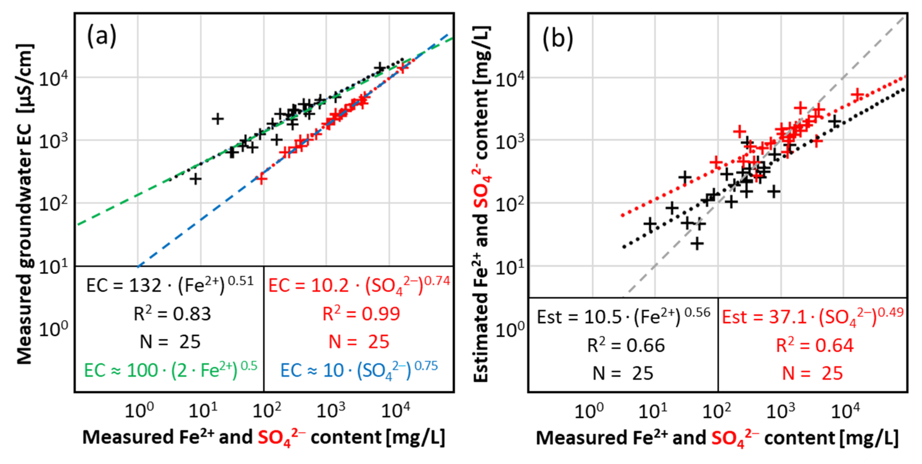
3.3.4. Groundwater Fe2+ and SO42− Content

The analysis of 25 groundwater samples (Table A4) shows that groundwater EC [µS/cm] appears to correlate on the log–log scale with dissolved iron (Fe2+) and sulfate (SO42−) content [mg/L], which is displayed in Figure 17a. The ratios between the EC values calculated from (Equation (2))
EC = 131.67∙(Fe2+)0.5131, EC = 10.229∙(SO42+)0.7441
and the EC values measured in situ are, on average, EC(Fe2+)/EC(Fe2+)meas = 1.05 ± 0.29 and EC(SO42−)/EC(SO42−)meas = 1.00 ± 0.09. Applying somewhat simplified relationships (Equation (3))
EC ≈ 100∙(2∙Fe2+)1/2, EC ≈ 10∙(SO42−)3/4
provides similar results: EC(Fe2+)/EC(Fe2+)meas = 1.05 ± 0.30 and EC(SO42−)/EC(SO42−)meas = 1.02 ± 0.09. Since the differences are small, we use Equation (3) for further analyses. In order to estimate the content of Fe2+ and SO42− at the observation wells (N = 25), we rearrange Equation (3) and use the transformation EC [µS/cm] = F∙10,000/ρ [mg/L]:
Fe2+est = 10,000/2∙(F/ρ)2, SO42−est = (1000∙F/ρ)4/3.
Figure 17b displays the results using a formation factor of F = 4 and a resistivity at 90 m asl (ρ). The corresponding best-fit lines for the estimated vs. measured values deviate from the 1:1 line and the ratios are quite high on average: Fe2+est/Fe2+meas = 1.63 ± 1.89 and SO42−est/SO42−meas = 1.35 ± 1.32. Using Equation (4) to estimate the distribution of Fe2+ and SO42− content in groundwater at 90 m asl throughout the survey area results in maps similar to that shown in Figure 14 with Fe2+est and SO42−est (instead of ρ) color scales.

4. Discussion

4.1. Methodological Validation

4.1.1. Positioning and Elevations

In an airborne geophysical survey, the spatial allocation of the measured data to the position of the geophysical sensors is of great importance. The BGR helicopter system enables this by using GPS receivers in the helicopter and in the bird as well as using an altimeter and an inclinometer in the bird to record the GPS position and the distance to the ground, respectively. This is important for the Finsterwalde survey, as the terrain surface in the mining area as well as the water levels in the post-mining lakes have changed over time and the digital elevation models did not correctly reflect the surface elevation everywhere at the time of the survey. Therefore, we used a hybrid terrain elevation, which mainly refers to a DEM outside the mining area, especially where forests occur, which was derived from the flight data inside the mining area. All resistivity cross-sections and depth slices refer to this elevation. In turn, the corrected terrain elevation helped to check and correct the measured bird altitude. Without these corrections, 1D HEM inversion models and their elevation would be strongly affected by false bird altitudes.

4.1.2. Resistivity Distribution

The resistivity pattern in the survey area can basically be divided into two areas (Figure 14). Within the mining area, generally, lower resistivities dominate, which are apparently caused by the deposition and rearrangement of fine-grained sediments and more highly mineralized lake and groundwater. Outside the mining area, the resistivities are significantly higher, indicating rather sandy subsoil and only slightly mineralized groundwater. The areas with lower resistivities there, which mostly run from east to west and correlate with river courses, are most likely due to deposited clayey sediments; however, outflow from the mining area cannot be excluded.

4.1.3. Water Table Estimation

The knowledge of the water levels of the lakes is important for the estimation of the water table in the entire survey area, as both are connected to each other. The HEM inversion models best reveal the water table if it is not too deep and is covered by dry and sandy sediments. In this way, there is a clear contrast between higher (vadose zone) and lower resistivities (water-saturated zone). In the Finsterwalde survey area, however, lower resistivities can occur at shallow depths, for example, in river lowlands and bogs, but also in the mining areas. In addition, the resistivities at the surface of the lakes, where increased water temperatures are to be expected, tend to be lower than below. A first attempt using the thickness of the cover layer derived from homogeneous half-space and 1D inversion did not lead to satisfactory results (Table 2), since the apparent depth at the highest frequency, which also serves as the initial value for the cover layer thickness of the 1D inversion, did not prove to be good enough. As explained for a two-layer case [42], the apparent depth tends to the cover layer thickness only if (i) the resistivity of the upper layer is many times greater than that of the lower layer and (ii) the centroid depth is much greater than the apparent depth. These assumptions often do not hold true in the survey area and the water table was generally estimated at shallower depths. Therefore, the maximum apparent depth dam (at all frequencies) was used instead, which often provided better results, but this was not everywhere due to deeper layers of fine-grained sediments (Figure 10a). The second attempt using standard (approach I) and modified (approach II) smooth inversion models in combination with a steepest gradient search led to significantly better results, but only for approach II (Table 3, Figure 10b). The water table estimated from airborne measurements can help to predict the possible flow directions of contaminated groundwater from the mining area. According to Figure 11, these are to be expected in a westerly direction, in line with the river courses.

4.1.4. Contamination of Lakes and Groundwater

The apparent resistivities at the highest frequency were used to estimate the contamination of the post-mining lakes (Figure 12). For this, an accurate calibration of the HEM system is essential, which was checked using the highest frequency data in comparison with water samples. The results showed that the calibration of the HEM system and the transformation based on a homogeneous half-space model were satisfactory—at least for the highest frequency HEM data relevant here. Therefore, the results presented in Figure 12 can be used to estimate the resistivity in the lakes as an approximation for the water quality, at least for the larger lakes. For smaller or shallow lakes, however, a 3D inversion is required to obtain accurate water quality parameters.
The comparison of the estimated groundwater resistivities derived from the HEM results with borehole data (Figure 16) shows that there is a fundamental uncertainty: The HEM resistivities depend not only on the mineralization of the groundwater, but also on the lithology, especially if clayey sediments occur in the vicinity of the well screens.
The uncertainty described above must of course also be taken into account in the further interpretation of the HEM results with regard to the estimation of Fe2+ and SO42− content in groundwater. We assume that a clear correlation between EC and dissolved Fe2+ or SO42− in groundwater can only be observed in post-mining landscapes such as Lusatia, where pyrite weathering dominates other contamination processes. However, these approximations cannot be applied to the lakes, as the lake waters are affected by inflowing water from different external sources, and no clear correlations between Fe2+ or SO42− content and the EC values were found. Outside the mining area, where the contamination of groundwater by Fe2+ or SO42− is generally lower, the significance of other, particularly non-mining, contaminants and the effect of lithology on resistivity values must also be considered.

4.2. Comparison with Ground Data

Despite careful data processing, there are still some uncertainties in determining the location and estimating groundwater-related parameters. The greatest differences in elevation to the DEM (up to several meters, Figure 5) occur in the post-mining lakes, as these have been flooded for several years. In other places, spoil heaps have been removed and leveled. While the terrain elevations derived from the flight data appear more reliable in these cases, the interpolation between the flight lines (250 m line spacing, 50 m grid cell size) causes uncertainties there that cannot be further reduced. This is also true for the resistivity grids, but due to the footprint of the HEM system, the lateral resolution is limited and the survey parameters are appropriate. This is acceptable for large-scale groundwater investigations.
The inversion of AEM data always provides resistivity models, which can be ambiguous and uncertain. However, the biggest source of error is the quality of the processed data [49,50]. Therefore, we have focused on reducing the data errors and using smoothed models in which data errors have less influence. Of course, this also reduces the vertical resolution, which affects the determination of interfaces (e.g., water table) and their comparison with borehole data. Thus, the HEM results shown here (smoothed spatial model data) are compared with reference data (point data), which have a much higher accuracy locally, but are only available at a few locations. Nevertheless, quite high correlations have been achieved, as the groundwater parameters considered (water table, EC values, and Fe2+/SO42− content) are also rather smoothly distributed.
Despite the high correlations already observed, it is important to take a critical look at the reference data used for comparison. This is illustrated, for example, by the assessment of the derived water table. The mean deviations from the water table belonging to the regional aquifer (Table 2, ∆dam_sel = 1.8 ± 3.9 m, Table 3, ∆SGE-II_sel = −0.7 ± 3.3 m) are of the same order as the differences between calculated and measured surface elevations at the selected sites (Table 3, ∆Topo-SE_sel = 0.7 ± 2.2 m). A further improvement in the statistic values (e.g., for ∆SGE-II_sel = −0.4 ± 2.6 m) would be possible with the exclusion of some further samples. These are five sample points at the edge of the survey area in the southeast, where the grid shown in Figure 11 was extrapolated, and two sample points at small lakes, where the SGE results were not automatically replaced due to the terrain elevation.
A further uncertainty can occur if the distance between the groundwater sample locations and the flight lines or the depth sections under consideration is too large. This is less critical if the resistivities change only slightly within these distances. This is usually the case for the horizontal distances, as the locations of the reference data are mostly within the HEM footprint, which is ensured by the half profile distance (approx. 125 m). For the vertical distances, it can be more critical, e.g., if a lithology change takes place near the filter section, which influences the HEM results but not the in situ data. We have checked this for the estimation of the formation factor (Section 3.3.3). Since the well screens are not always located close to the considered elevation of 90 m asl (Figure 14), a change in lithology cannot be excluded. Using only the water samples for well screen depths of 90 ± 10 m asl, the resulting formation factor is only slightly changed (F = 4.3 ± 1.7, N = 20) compared to the previous result (F = 4.3 ± 1.9, N = 25). This shows that it is not the vertical distance, but rather an inhomogeneous lithology that leads to the observed scatter.
In general, only one chemical indicator can be derived from one HEM parameter (here, this is EC derived from resistivity (at 90 m asl) assuming F = 4 and neglecting lithological differences). Since iron and sulfate are often used to characterize water quality in post-mining landscapes and show a high correlation with EC values in groundwater (Figure 17), we use both parameters. The correlation between Fe2+ and SO42− is also high (R2 = 0.85). All other chemical indicators show significantly lower correlations. The use of the approximate values in Equations (3) and (4) is appropriate, as the differences to the use of the calculated regression coefficients are small. The largest uncertainty arises from the smoothed resistivity distribution (ρ at 90 m asl) and the formation factor F. We have assumed that sandy sediments dominate in the areas of the well screens and used F = 4. Although this is mostly true, clayey sediments exist above and below the well screens at some borehole locations, which affect the HEM results but not the in situ measurements. The application of a lower but still constant formation factor of F = 3 (typical for clayey sand) leads to a downshift of the estimated values, as shown in Figure 17b, and significantly lower ratios, which are, on average, as follows: Fe2+est/Fe2+meas = 0.91 ± 1.06 (instead of 1.63 ± 1.89) and SO42−est/SO42−meas = 0.92 ± 0.90 (instead of 1.35 ± 1.32). The standard deviation of the ratios is still high and the slopes of the best-fit lines remain unchanged. Therefore, we also checked the residuals. Two extreme values occur for wells located at the edge of the mining area or close to the Bergheider See (Well No 20 and 23 in Table A4). Very low Fe2+ and SO42 values were measured there. Repeating the statistical analyses without these two wells results in Fe2+est/Fe2+meas = 1.15 ± 0.96 and SO42−est/SO42−meas = 0.99 ± 0.49 and the R2 values are slightly higher (R2 (Fe2+) = 0.72 and R2 (SO42−) = 0.73). We have to assume that neither changing the constant formation factor nor omitting some local reference data is sufficient to achieve high correlations between estimated (from HEM) and measured well data, as there are principally differences between large-scale HEM resistivities and local in situ measurements. Particularly, in the case of a smooth HEM inversion, it should be noted that thin (lithological or hydrogeological) layers with strongly varying resistivities appear flattened. Consequently, a comparison with discrete borehole data leads to a flattening of the fit line of a linear regression.

5. Conclusions

The focus of the study described here was the investigation of a post-mining landscape in the Lusatian mining district, which used helicopter-borne electromagnetics to obtain information about the aquifers, their depth, and pore water mineralization. With the airborne survey, the post-mining landscape could be mapped over a large area and in a relatively short time without having to enter the partially inaccessible terrain. This is a clear advantage of airborne over ground-based geophysical surveys, which often have to be limited to smaller survey areas and specific questions.
The first airborne electromagnetic survey carried out in this former opencast lignite mining region provided the spatial resistivity distribution with the following benefits:
  • The regional water table was derived from the HEM resistivity models, which could be verified by measurements in lakes and boreholes.
  • Significant variations in the water conductivity of the post-mining lakes were mapped using the apparent resistivities at the highest system frequency. For the larger lakes, the results are in good agreement with the conductivity measurements in the lakes. For smaller lakes, however, more detailed measurements (reduced flight line separation) and complex evaluations (modeling) are required.
  • Water analyses in the study area showed that the electrical conductivity in the groundwater correlates with the content of dissolved Fe2+ and SO42−. This content could be estimated from airborne resistivity data at 90 m asl within the entire area of the former mining site. The results using a formation factor of F = 4 can be improved with the help of—if available—more borehole data (lithology) and improved techniques (e.g., machine learning), in order to better take into account the contribution of lithology to electrical conductivity and the distribution of the formation factor. However, here we have focused on using the borehole data only to verify the airborne results.
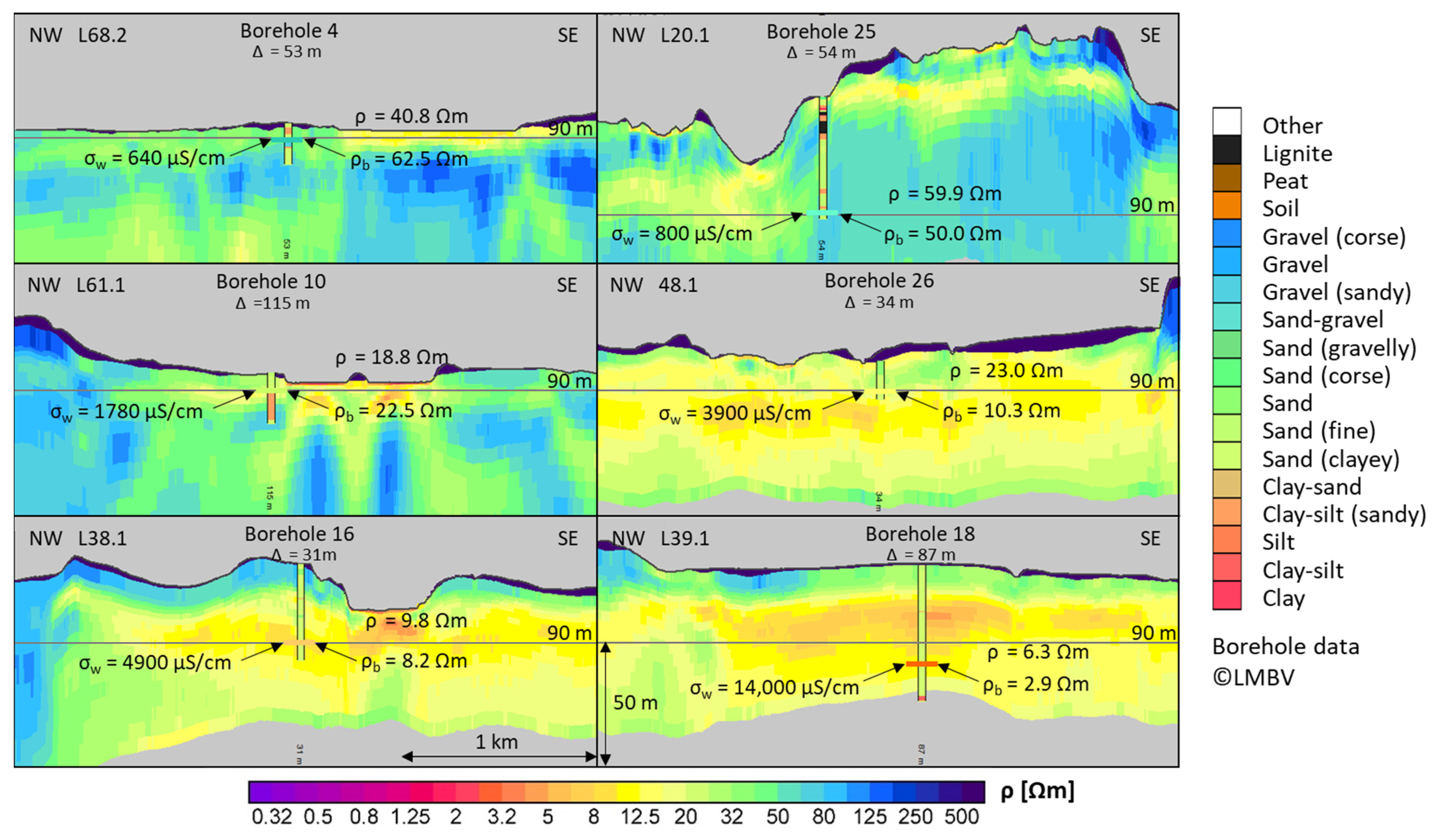
  • The airborne results can also be used to close data gaps between boreholes, where information on the (hydro-)geological subsurface is often limited.
  • The results of non-invasive airborne surveys are well suited for the (hydro-)geological description of post-mining landscapes. Once the airborne geophysical results have been evaluated, a uniform and extensive dataset is available that can be used to obtain valuable information on the (hydro-)geological subsurface conditions.
  • The data resulting from the geophysical investigations can also be used as baseline data for further evaluation, interpretation, and modeling.

Supplementary Materials

The following supporting information can be downloaded at https://www.mdpi.com/article/10.3390/w17071000/s1: Lithology data S1: Lithology.dat.

Author Contributions

Conceptualization, B.S.; methodology, B.S.; software, B.S.; validation, B.S., O.C.A., S.J. and E.N.; formal analysis, B.S.; investigation, B.S.; resources, B.S., O.C.A., S.J. and E.N.; data curation, B.S., O.C.A., S.J. and E.N.; writing—original draft preparation, B.S., S.J. and E.N.; writing—review and editing, B.S., O.C.A., S.J. and E.N.; visualization, B.S. and S.J.; supervision, B.S.; project administration, B.S. and S.J.; funding acquisition, B.S. and S.J. All authors have read and agreed to the published version of the manuscript.

Funding

This research received no external funding.

Data Availability Statement

The data are available in a publicly accessible repository: Raw Data on Helicopter-borne Electromagnetics (HEM) Area 191 Finsterwalde comprises the following zip file: 191FinsterwaldeHEM-RD.zip, accessible from following the link: https://doi.org/10.25928/zb8x-ke65. Helicopter-borne Electromagnetics (HEM) Area 191 Finsterwalde comprises the following zip file: 191FinsterwaldeHEM.zip, accessible from following the link: https://doi.org/10.25928/t7pz-1369. The following dataset is available on request from the authors: Inversion Models derived from Helicopter-borne Electromagnetics (HEM) Area 191 Finsterwalde. In terms of the third party data, all in situ measurements have been provided by LMBV [46]. LMBV has agreed to the publication of the data presented in the figures, in Appendix A, and provided in Supplementary Materials (27 January 2025). Information on the terms of use for the following download products: [31]: “dl-de/by-2-0” referring to the licence text available at www.govdata.de/dl-de/by-2-0); [32,33]: Adapted with permission from LMBV (27 January 2025).

Acknowledgments

We would like to thank LMBV for providing geological and hydrogeological data for comparisons with the results of the airborne geophysical survey. We also thank the academic editor and two anonymous reviewers for their helpful suggestions to improve the paper.

Conflicts of Interest

The authors declare no conflicts of interest.

Abbreviations

The following abbreviations are used in this manuscript:
AEMAirborne Electromagnetic;
AMDAcid Mine Drainage;
BGRBundesanstalt für Geowissenschaften und Rohstoffe;
BKGBundesamt für Kartographie und Geodäsie;
DEMDigital Elevation Model;
ECElectrical Conductivity;
GNSSGlobal Navigation Satellite System;
GPSGlobal Positioning System;
HEMHelicopter-borne Electromagnetic;
IMUInertial Measurement Unit;
I, QIn-phase, Quadrature of HEM data;
LBGRLandesamt für Bergbau, Geologie und Rohstoffe Brandenburg;
LfULandesamt für Umwelt Brandenburg;
LMBVLausitzer und Mitteldeutsche Bergbau-Verwaltungsgesellschaft mbH;
PPPPrecise Point Positioning;
SG(E)Depth (Elevation) of Steepest Gradient;
TopoTerrain elevation.

Appendix A

Appendix A.1

Table A1. Measured lake water levels (LMBV [46]) in comparison with estimated water tables derived from airborne data (approaches I + II, deselected values in italics).
Lake
No
Northing
[UTM33]
Easting
[UTM33]
Water Level
[m asl]
Est. Water Table
Appr. I [m asl]
Est. Water Table
Appr. II [m asl]
14160805714196107.58107.27107.60
24248755713288119.02113.61119.15
3409268570831092.9490.7693.39
4407034570521092.5288.7692.41
5408457570802392.6188.6393.36
64114215711155101.2997.9798.89
74105085711137101.5694.5999.07
84130985712787102.66102.72102.81
94232445713485119.34119.53120.15
10408881570843692.6791.2593.53
114123805710877100.56100.61100.54
12412320570909999.3393.8198.66
13411036570843497.4493.4898.10
14407034570779692.5291.8392.72
15405223570587194.2091.6694.88
16404084570504696.3293.4398.76
174196915714071138.94113.21120.83
184186325708286119.80107.02107.28
19409946570817393.7090.8094.88
20407158570648692.5289.5492.09
214127385707365104.8495.52100.85
22407088570432292.2186.4691.98
23405510570763192.5290.2392.80
244226705714770123.43122.12121.07
25410822570460292.6289.7393.22
26410414570499492.6587.8292.59
274130045708472103.8193.12101.80
28406637570414591.9988.8292.70
294212735714449128.81123.17122.73
304153965711040109.43107.57110.52
314178065715149148.84111.91117.54
324161075716223120.51104.89106.81
334101565711775102.4394.7197.34
344146765713710105.02101.66105.59
354142545709584105.59101.00104.21
364171065710541110.74107.71111.20
374155945711462112.43107.27113.10

Appendix A.2

Table A2. Water tables measured in boreholes (LMBV [46]) in comparison with estimated water tables derived from airborne data (approaches I + II, deselected values in italics).
Well
No
Northing
[UTM33]
Easting
[UTM33]
Water Table
[m asl]
Est. Water Table
Appr. I [m asl]
Est. Water Table
Appr. II [m asl]
1407023570411192.2286.5091.98
24196415708364106.83100.66106.21
34240995713756127.58120.44123.11
44145305715447107.94104.46104.06
54105535715591104.7694.8098.46
64152735713126107.62102.52108.03
74151125712697107.62102.73108.95
84150185712387107.94103.53109.61
94145855711045107.20106.06109.33
104190255713775137.56112.89119.45
114115775708382101.3394.8499.76
124147485714660107.32103.37104.80
134132955712061105.08102.99104.12
144129035711042103.17102.08101.47
154190535709379108.73109.60112.57
164191435711416112.57111.13118.39
174144955710654106.78105.21107.88
184201175708736106.5399.50110.15
194130015707117104.5695.40100.84
204119805710188101.6799.24100.64
214154555711643109.08106.84112.89
224210085706491101.1297.7197.92
234126075708680101.8293.18101.16
244124715709368101.1995.25100.80
254206435709384106.99103.85114.87
264207645709708106.97106.10116.85
274208785710433109.81111.34119.50
284130245707640104.0095.28101.24
294131665707696103.6595.37101.29
304131565708749103.7892.45102.02
314128585708433102.5893.32101.64
324169565712960109.29110.77113.02
334200065707440104.2896.67100.63
344145955709969106.87104.34106.98
354131395707506104.2495.52101.11
364110465708197100.4693.5098.87
374127865711663103.37102.20102.45
384136595713096104.85103.71104.49
394121885709852101.2898.54100.87
404226175710566118.71108.86112.60
414154095715924109.15104.58104.84
424108535708987100.6093.5899.67
434113715708068101.2594.6199.53
444115885708093101.6495.3299.98
454113865708190101.1994.5599.58
464131415707709103.7095.31101.31
474132045707818104.7395.28101.43
484131455707679103.6895.36101.27
494131325707357104.6295.51101.01
504123945707406103.4896.22100.37
514231335710928119.15107.73113.56
524228365710873119.51108.67113.48
53407584570463192.3685.8291.37
54410542570815498.2792.1797.05
554138625715540107.88104.37104.01
564157805716217113.08104.50105.76
574159985715885109.08105.48106.19
584131815714410106.65104.08105.41
594168975714958108.69108.69110.60
604142125715417107.90104.57103.80
614138375714737107.36103.85103.90
62409822570924897.9594.1997.00
634150255715942108.89104.17104.00
644152445715783109.10104.53104.63
654152245715781109.06104.51104.60
664153105715647108.90104.74104.88
67406466570682793.7590.2493.64
684147085713135107.13101.88107.04
69408711570848695.7391.7094.67
70408724570834695.3490.7994.59
71408688570825393.6390.2094.02

Appendix A.3

Table A3. Water EC measured in lakes (LMBV [46]) converted to resistivity ρw in comparison with apparent resistivities ρa (f = 128 kHz) derived from airborne data (picked from grid or next flight line). Additional parameters: Approximate distance of the sampling location to the lakeshore and maximum width of the lakes.
Lake
No
Northing
[UTM33]
Easting
[UTM33]
EC
[µS/cm]
ρw
[Ωm]
ρa (Grid)
[Ωm]
ρa (Line)
[Ωm]
Distance
[m]
Width
[m]
1415912571446420104.985.014.904501200
2413203571269031103.224.113.50100600
3412405571120032403.092.592.90250500
4411918571148032403.096.413.20100400
5410759571095227303.6624.994.2050200
6412058570919633303.007.823.0050400
7414015570962413507.4127.7113.6050140
8410774570822833702.9714.634.0050140
9413041570867194510.5821.1321.9050100
10407217570803678812.6913.8613.50250800
11405861570773267114.9019.4318.9070120
12408857570806626003.8516.575.1010180
13408717570814031203.2116.957.2010100
14408007570746532003.1221.1215.001060
15407218570650229803.363.133.20130350
16407043570513225303.954.734.10250300
17405060570566927303.6615.606.3050120
18406960570449323704.2210.7511.001060
19419735571420137926.3929.0727.00100400
20424912571307620704.834.144.50240600
21423374571320290811.0125.6012.4050450
22412847570738923804.207.704.1010400

Appendix A.4

Table A4. Groundwater EC (converted to resistivity ρw) and Fe2+ and SO42− content in observation wells (LMBV [46]) in comparison with resistivities ρ derived from airborne data (picked from resistivity grid at 90 m asl) and estimated Fe2+ and SO42− content (deselected values in italics).
Well
No
Northing
[UTM33]
Easting
[UTM33]
EC
[µS/cm]
ρw
[Ωm]
ρ (90 m asl)
[Ωm]
Fe2+
[mg/L]
SO42−
[mg/L]
Est. Fe2+
[mg/L]
Est. SO42−
[mg/L]
1412857570843310299.4327.82162511103753
2420131571142718535.4616.7413810302851483
3420965571092630003.3715.0531820003531709
4421150571347676413.1626.8967329111788
5407545570733063815.6240.773225748453
6408541571382399310.3141.585138146441
7411677571079629203.4417.5647020402591391
8414595570996936502.7814.8753525503621736
9411046570819724004.2019.2128216102171234
10408817570874717905.6218.8028711002261270
11418061571170626203.7720.5118113801901131
12410132571111521204.8822.972851330152972
13410638571086722004.6930.9719128083653
14410935571064312607.8724.4787690134894
15412659571293048102.049.75139040508423048
16414757571183430203.339.3329620409193233
174155115709795141500.716.3471601660019905411
18405339570549425404.0016.1124514103081561
19411662570897526003.8515.9653417603141580
20410526570804665017.5417.79302212531367
21414960571467337402.7013.5143527904381973
22415597571262943602.3311.6980335905852393
23417129571402624741.4941.5789346441
24416896571495980212.5059.924740522271
25412690570926338702.5623.057703730151968

References

  1. von Bismarck, F. Land in motion–opencast restoration and recultivation in Lusatia. In Post-Mining Landscape, Conference Documentation; Internationale Bauausstellung (IBA) Fürst-Pückler-Land, Ed.; Jovis: Berlin, Germany, 2010; pp. 37–41. ISBN 978-3-86859-043-2. [Google Scholar]
  2. Krümmelbein, J.; Bens, O.; Raab, T.; Anne Naeth, M. A history of lignite coal mining and reclamation practices in Lusatia, eastern Germany. Can. J. Soil Sci. 2012, 92, 53–66. [Google Scholar] [CrossRef]
  3. Drebenstedt, C.; Kuyumcu, M. (Eds.) Braunkohlesanierung: Grundlagen, Geotechnik, Wasserwirtschaft, Brachflächen, Rekultivierung, Vermarktung; Springer: Berlin/Heidelberg, Germany, 2014. [Google Scholar] [CrossRef]
  4. Benthaus, F.-C.; Totsche, O. The groundwater raise in lignite mining induced areas in Lusatia–actions taken to reduce the follows ups. Min. Rep. 2015, 151, 522–530. Available online: https://mining-report.de/wp-content/uploads/2015/11/MiRe_1506_Grundwasserwiederanstieg_151124.pdf (accessed on 12 February 2025).
  5. Frei, S.; Klostermann, L.; Gilfedder, B.S. Iron retention in Lusatia: A spatially differentiated analysis of the Spree. Grundwasser 2024, 29, 213–228. [Google Scholar] [CrossRef]
  6. Schultze, M.; Pokrandt, K.-H.; Hille, W. Pit lakes of the Central German lignite mining district: Creation, morphometry and water quality aspects. Limnologica 2010, 40, 148–155. [Google Scholar] [CrossRef]
  7. Gläßer, C.; Groth, D.; Frauendorf, J. Monitoring of hydrochemical parameters of lignite mining lakes in Central Germany using airborne hyperspectral casi-scanner data. Int. J. Coal Geol. 2011, 86, 40–53. [Google Scholar] [CrossRef]
  8. Bamisaiye, O.A. Subsurface mapping: Selection of best interpolation method for borehole data analysis. Spat. Inf. Res. 2018, 26, 261–269. [Google Scholar] [CrossRef]
  9. Gondolfo, O.C.B. Determination of water table depth using geophysical methods. Braz. J. Geophys. 2022, 40, 1–15. [Google Scholar] [CrossRef]
  10. King, A.R.; Hynes, T. Applications of geophysical methods for monitoring acid mine drainage. In Proceedings of the International Land Reclamation and Mine Drainage Conference and the Third International Conference on the Abatement of Acidic Drainage, Pittsburgh, PA, USA, 24 April 1994; pp. 317–326. [Google Scholar] [CrossRef]
  11. Shokri, B.J.; Ardejani, F.D.; Ramazi, H.; Moradzadeh, A. Predicting pyrite oxidation and multi-component reactive transport processes from an abandoned coal waste pile by comparing 2D numerical modeling and 3D geo-electrical inversion. Int. J. Coal Geol. 2016, 164, 13–24. [Google Scholar] [CrossRef]
  12. Moreira, C.A.; Casagrande, M.F.S.; Büchi, F.M.S.; Targa, D.A. Hydrogelogical characterization of a waste rock pile and bedrock affected by acid mine drainage from geophysical survey. SN Appl. Sci. 2020, 2, 1236. [Google Scholar] [CrossRef]
  13. Kirsch, R. (Ed.) Groundwater Geophysics—A Tool for Hydrogeology; Springer: Berlin, Heidelberg, Germany, 2006. [Google Scholar] [CrossRef]
  14. Paine, J.G.; Minty, B.R.S. Airborne hydrogeophysics. In Hydrogeophysics; Rubin, Y., Hubbard, S.S., Eds.; Springer: Dordrecht, The Netherlands, 2005; pp. 333–357. [Google Scholar] [CrossRef]
  15. Siemon, B.; Ibs-von Seht, M.; Steuer, A.; Deus, N.; Wiederhold, H. Airborne electromagnetic, magnetic, and radiometric surveys at the German North Sea coast applied to groundwater and soil investigations. Remote Sens. 2020, 12, 1629. [Google Scholar] [CrossRef]
  16. Harrison, E.J.; Baranwal, V.C.; Pfaffhuber, A.A.; Christensen, C.W.; Skurdal, G.H.; Rønning, J.S.; Anschütz, H.; Brönner, M. AEM in Norway: A Review of the Coverage, Applications and the State of Technology. Remote Sens. 2021, 13, 4687. [Google Scholar] [CrossRef]
  17. Knight, R.; Smith, R.; Asch, T.; Abraham, J.; Cannia, J.; Viezzoli, A.; Fogg, G. Mapping aquifer systems with airborne electromagnetics in the Central Valley of California. Groundwater 2018, 56, 893–908. [Google Scholar] [CrossRef]
  18. Jørgensen, F.; Møller, M.M.; Nebel, L.; Jensen, N.-P.; Christiansen, A.V.; Sandersen, P.B.E. A method for cognitive 3D geological voxel modelling of AEM data. Bull. Eng. Geol. Environ. 2023, 72, 421–432. [Google Scholar] [CrossRef]
  19. Høyer, A.-S.; Jørgensen, F.; Foged, N.; He, X.; Christiansen, A.V. Three-dimensional geological modelling of AEM resistivity data—A comparison of three methods. J. Appl. Geophys. 2015, 115, 65–78. [Google Scholar] [CrossRef]
  20. Marker, P.A.; Foged, N.; He, X.; Christiansen, A.V.; Refsgaard, J.C.; Auken, E.; Bauer-Gottwein, P. Performance evaluation of groundwater model hydrostratigraphy from airborne electromagnetic data and lithological borehole logs. Hydrol. Earth Syst. Sci. 2015, 19, 3875–3890. [Google Scholar] [CrossRef]
  21. King, J.; Mulder, T.; Essink, G.O.; Bierkens, M.F.P. Joint estimation of groundwater salinity and hydrogeological parameters using variable-density groundwater flow, salt transport modelling and airborne electromagnetic surveys. Adv. Water Res. 2022, 160, 104118. [Google Scholar] [CrossRef]
  22. Siemon, B.; Christiansen, A.V.; Auken, E. A review of helicopter-borne electromagnetic methods for groundwater exploration. Near Surf. Geophys. 2009, 7, 629–646. [Google Scholar] [CrossRef]
  23. Auken, E.; Boesen, T.; Christiansen, A.V. Chapter Two—A review of airborne electromagnetic methods with focus on geotechnical and hydrological applications from 2007 to 2017. Adv. Geophys. 2017, 58, 47–93. [Google Scholar] [CrossRef]
  24. Hammack, R.; Love, E.; Veloski, G.; Ackman, T.; Harbert, W. Using helicopter electromagnetic surveys to identify environmental problems at coal mines. Mine Water Environ. 2003, 22, 80–84. [Google Scholar] [CrossRef]
  25. Love, E.; Hammack, R.; Harbert, W.; Sams, J.; Veloski, G.; Ackman, T. Using airborne thermal infrared imagery and helicopter EM conductivity to locate mine pools and discharges in the Kettle Creek watershed, north-central Pennsylvania. Geophysics 2005, 70, B73–B91. [Google Scholar] [CrossRef]
  26. Demirel, N.; Emil, M.K.; Duzgun, H.S. Surface coal mine area monitoring using multi-temporal high-resolution satellite imagery. Int. J. Coal Geol. 2011, 86, 3–11. [Google Scholar] [CrossRef]
  27. Schroeter, L.; Gläβer, C. Analyses and monitoring of lignite mining lakes in Eastern Germany with spectral signatures of Landsat TM satellite data. Int. J. Coal Geol. 2011, 86, 27–39. [Google Scholar] [CrossRef]
  28. Siemon, B.; Ibs-von Seht, M.; Pielawa, J. Gebietsbericht D-AERO-Finsterwalde HEM/HMG/HRD-Befliegung 191 Finsterwalde Mai/Juli 2021; Bundesanstalt für Geowissenschaften und Rohstoffe: Hannover, Germany, 2022. [Google Scholar] [CrossRef]
  29. LBGR. Geologische Übersichtskarte 1:100000 (GÜK100); Landesamt für Bergbau, Geologie und Rohstoffe: Cottbus, Germany, 2015; Available online: https://geo.brandenburg.de/?page=Geologische-Karten (accessed on 11 November 2024).
  30. BKG. Digitale Topographische Karte 1:1000000 (DTK1000); Bundesamt für Kartographie und Geodäsie: Frankfurt, Germany, 2021; Topographic Map Generated From: Spatial Data Base: ©GeoBasis-DE/BKG (2021); Available online: https://gdz.bkg.bund.de/index.php/default/catalog/product/view/id/1454/s/digitale-topographische-karte-1-100-000-dtk100 (accessed on 11 November 2024).
  31. LfU. Gewässernetz; Landesamt für Umwelt Brandenburg: Potsdam, Germany, 2024; Available online: https://data.geobasis-bb.de/geofachdaten/Wasser/Hydrologie/gewnet25.zip (accessed on 11 November 2024).
  32. LMBV. Bergbaufolgeseen; Lausitzer und Mitteldeutsche Bergbau-Verwaltungsgesellschaft mbH: Senftenberg, Germany, 2024; Available online: https://lmbv.maps.arcgis.com/apps/webappviewer/index.html?id=64068d71103d40a9a0a07f6b0682db1c&extent=1425029.5094%2C6647119.0691%2C1718547.698%2C6795254.0299%2C102100&showLayers=Wasser_View_5083%3BUeberleiter_View_2598 (accessed on 11 November 2024).
  33. LMBV. Landinanspruchnahme; Lausitzer und Mitteldeutsche Bergbau-Verwaltungsgesellschaft mbH: Senftenberg, Germany, 2024; Available online: https://geodatenportal-lmbv.hub.arcgis.com/maps/62bfad18b48244eebc81bca44f337cb8 (accessed on 11 November 2024).
  34. Standke, G.; Rascher, J.; Volkmann, N. Lowstand cycles and coal formation in paralic environments: New aspects in sequence statigraphy. In Northern European Cenozoic Stratigraphy—Proceedings of the 8th Biannual Meeting of the RCNNS/RCNPS; Guers, K., Ed.; Landesamt für Natur und Umwelt des Landes Schleswig-Holstein: Flintbek, Germany, 2002; pp. 153–161. [Google Scholar]
  35. Barth, W.; Bönisch, R.; Krentz, O.; Kühner, R.; Lapp, M.; Petzold, H.; Schneider, W.; Schulze, H.; Seibel, B.; Standke, G. Die geologische Entwicklung der Lausitz; Vattenfall Europe Mining AG: Cottbus, Germany, 2010. [Google Scholar]
  36. Stackebrandt, W.; Franke, D. Geologie von Brandenburg; Schweizerbart Science Publishers: Stuttgart, Germany, 2015; ISBN 978-3-510-65295-2. [Google Scholar]
  37. LfU. Grundwassermessnetz; Landesamt für Umwelt Brandenburg: Potsdam, Germany; Available online: https://maps.brandenburg.de/WebOffice/synserver?project=GWM_www_CORE (accessed on 14 February 2025).
  38. Christiansen, A.V.; Auken, E. A global measure for depth of investigation. Geophysics 2012, 77, WB171–WB177. [Google Scholar] [CrossRef]
  39. Tølbøll, R.J.; Christensen, N.B. Sensitivity functions of frequency-domain magnetic dipole-dipole systems. Geophysics 2007, 72, F45–F56. [Google Scholar] [CrossRef]
  40. Siemon, B.; van Baaren, E.; Dabekaussen, W.; Delsman, J.; Dubelaar, W.; Karaoulis, M.; Steuer, A. Automatic identification of fresh-saline groundwater interfaces from airborne electromagnetic data in Zeeland, the Netherlands. Near Surf. Geophys. 2019, 17, 3–25. [Google Scholar] [CrossRef]
  41. Siemon, B.; Steuer, A.; Ullmann, A.; Vasterling, M.; Voß, W. Application of frequency-domain helicopter-borne electromagnetics for groundwater exploration in urban areas. Phys. Chem. Earth 2011, 36, 1373–1385. [Google Scholar] [CrossRef]
  42. Siemon, B. Improved and new resistivity-depth profiles for helicopter electromagnetic data. J. Appl. Geophys. 2001, 46, 65–76. [Google Scholar] [CrossRef]
  43. Sengpiel, K.-P.; Siemon, B. Advanced inversion methods for airborne electromagnetic exploration. Geophysics 2000, 65, 1983–1992. [Google Scholar] [CrossRef]
  44. Annetts, A.; George, R.; Munday, T.; Ibrahimi, T.; Cahill, K.; Paul, R.; Davis, A. The application of AEM to mapping sea-water intrusion at La Grange, WA. In Proceedings of the ASEG-PESA 2015, Perth, Australia, 15–18 February 2015. [Google Scholar] [CrossRef]
  45. BKG. Digitales Geländemodel (DGM25); Bundesamt für Kartographie und Geodäsie: Frankfurt, Germany, 2021; Spatial Data Base: ©GeoBasis-DE/BKG (2021); Available online: https://gdz.bkg.bund.de (accessed on 1 February 2012).
  46. LMBV. Lithology Data, Water Table Data, Hydrochemical Data; Personal communication; adapted with permission from LMBV (27 January 2025); Lausitzer und Mitteldeutsche Bergbau-Verwaltungsgesellschaft mbH: Senftenberg, Germany, 2022. [Google Scholar]
  47. Kang, S.; Knight, R.; Greene, T.; Buck, C.; Fogg, G. Exploring the model space of airborne electromagnetic data to delineate largescale structure and heterogeneity within an aquifer system. Water Resour. Res. 2021, 57, e2021WR029699. [Google Scholar] [CrossRef]
  48. Archie, G.E. The electrical resistivity log as an aid in determining some reservoir characteristics. Trans. AIME 1942, 146, 54–62. [Google Scholar] [CrossRef]
  49. Yin, C.-C.; Ren, X.-Y.; Liu, Y.-H.; Qi, Y.-F.; Qiu, C.-K.; Cai, J. Review on airborne electromagnetic inverse theory and applications. Geophysics 2015, 80, W17–W31. [Google Scholar] [CrossRef]
  50. Brodie, R.; Sambridge, M. Holistic inversion of frequency-domain airborne electromagnetic data with minimal prior information. Explor. Geophys. 2009, 40, 8–16. [Google Scholar] [CrossRef]
Figure 1. Examples of landscapes in the opencast lignite-mining district in Lusatia: (a) active opencast lignite mine, (b) nearby dump with towed helicopter-borne system, (c,d) post-mining lakes with contaminated water (photos taken in July 2021 by cameras attached to the bottom of the BGR helicopter).
Water 17 01000 g001
Figure 2. Geological overview map (left) and typical lithological units (right) of the survey area (after: [29,30,31,32,33]). The airborne survey area is shown in red.
Water 17 01000 g002
Figure 3. Flow chart showing processing steps for helicopter-borne electromagnetic (HEM), position (POS), and attitude (IMU) data. After the correction of the position data, coordinates (UTM) and sensor altitudes (Alt) together with the processed HEM data are used for inversion (homogeneous half-space and multi-layer 1D inversion). The product (terrain elevation (Topo), water table, apparent resistivity ρa at the highest HEM frequency, resistivity ρ at 90 m asl, and estimated Fe2+/SO42− content) are compared (see Figures) with the external reference data (borehole data, digital elevation model (DEM), lake water level (LWL), groundwater table (GWT), the electrical conductivity (EC) of lake and groundwater, and Fe2+/SO42− content in wells.
Water 17 01000 g003
Figure 4. Terrain elevations derived from flight data (Topo), corrected with the help of a digital elevation model (DEM, [45]) in areas without recent elevation changes. The grids (50 m cell size) are based on flight line data.
Water 17 01000 g004
Figure 5. Differences between Topo and DEM. The grids (50 m cell size) are based on flight line data. Flight lines are drawn in black.
Water 17 01000 g005
Figure 6. Apparent resistivities at each frequency of the HEM system. The corresponding mean depth values (±standard deviations) are approximately 4–11 m (f = 128 kHz), 6–15 m (f = 41 kHz), 14–28 m (f = 8.4 kHz), 16–32 m (f = 5.4 kHz), 28–53 m (f = 1.8 kHz), and 60–100 m (f = 0.4 kHz).
Water 17 01000 g006
Figure 7. Resistivity cross-sections along tie line T13.8 (location see Figure 5) for (a) the inversion with few layers and (b) the smooth inversion (approach I). The path (elevation) of the HEM system (bird), the topographic elevation (black line above the colored models), and the quality control parameter (QCP, white: high quality, red: low quality) of the HEM data are also shown.
Water 17 01000 g007
Figure 8. A resistivity cross-section of line L11.1 (location see Figure 5) for the smooth inversion with color-coded drilled lithology (data provided by LMBV [46]) on top (distance to L11.1 ≤ 50 m).
Water 17 01000 g008
Figure 9. A comparison of the estimated and measured [46] water tables using all (red) or selected (black) sample data. (a) Derived from the homogeneous half-space inversion (maximum apparent depth dam). (b) Derived from the modified smooth 1D inversion (SGE-II). The dotted lines indicate the best-fit lines; the dashed gray line indicates the 1:1 line.
Water 17 01000 g009
Figure 10. Resistivity cross-sections belonging to (a) approach I and (b) approach II along tie line T13.8 (for location see Figure 11) together with the estimated elevation of the water table (purple line) and samples (colored columns, after LMBV [46]) indicating the vadose zone (white), the water table (blue), and the saturated zone below. The maximum distance of the samples to the flight line is less than 350 m.
Water 17 01000 g010
Figure 11. Elevations of the estimated water table derived from smooth HEM models using approach II (grid) in comparison with water tables provided by LMBV [46]. These values (face color of the dots) belong to different aquifers (edge color of the dots). Rivers [31], lakeshores [32], mining area [33], and flight lines are marked. The grid (50 m cell size) is based on flight line data.
Water 17 01000 g011
Figure 12. Apparent resistivities (ρa) at the highest frequency of f = 128 kHz (map) compared to measured electrical conductivities (EC) of water (provided by LMBV [46]) after conversion to water resistivities (ρw) at sample points in lakes (dots). Rivers [31], lakeshores [32], mining areas [33], and flight lines are marked.
Water 17 01000 g012
Figure 13. Ratios of apparent resistivities at 128 kHz and resistivities of lake water [46]. (a,b): values picked from grids, (c,d): values picked on closest flight lines. Colors refer to the distance to the lakeshore. Dashed lines indicate the 1:1 line; dotted lines indicate 100 m and 200 m distance to lakeshore and lake width, respectively.
Water 17 01000 g013
Figure 17. (a) Groundwater EC vs. Fe2+ (black) and SO42− (red) content with calculated (doted) and estimated (dashed) trend lines. (b) Estimated Fe2+ (black) and SO42− (red) content derived from resistivities ρ at 90 m asl vs. Fe2+ (black) and SO42− (red) content in groundwater [46]. Dotted lines indicate the best-fit lines; dashed line indicates the 1:1 line.
Water 17 01000 g017
Table 1. Characteristics of primary data sources used within this study. The column “Time” describes the timestamp of the acquired information.
DatasetReferenceTypeExtentResolutionTime
DEMBKG [45]GridGermany25 m2012
TopographyBKG [30]PolylinesGermany-
Water table/levelLMBV [46]PointsLocal-2021-07
Water qualityLMBV [46]PointsLocal-2021-07
Stream topographyLfU [31]PolylinesBrandenburg-
Lake topographyLMBV [32]PolygonsBrandenburg-
Mining areaLMBV [33]PolylinesBrandenburg-
Borehole/well dataLMBV [46]PointsBrandenburg-
Table 2. Mean values (Δ) and standard deviations (σ) of differences in estimated elevations of water tables derived from da (f = 128 kHz), dam (maximum), d1(6) (6 layers), d1(20) (20 layers), and measured values [46] in lakes, wells, and both are listed. Statistical parameters excluding 19 samples belonging to perched aquifers or high (≥125 m asl) lake levels are indicated by “_sel”. For locations, see Table A1 and Table A2.
Elevation
Parameter
NumberLakes
Δ [m]
σ [m] NumberWells
Δ [m]
σ [m] NumberTotal
Δ [m]
σ [m]
da370.801.71 717.368.42 1085.117.56
da_sel340.671.54 555.666.44 893.755.68
dam370.321.97 713.876.69 1082.655.78
dam_sel340.251.89 552.694.56 891.763.94
d1(6)371.262.03 717.788.06 1085.547.32
d1(6)_sel341.101.81 556.146.45 894.225.73
d1(20)371.191.74 716.747.61 1084.836.77
d1(20)_sel340.791.91 556.056.49 894.045.81
Table 3. Mean values (Δ) and standard deviations (σ) of differences in estimated elevations of water tables (SGE-I, SGE-II) derived from steepest gradient analyses of 1D inversion models and measured values [46] in lakes, wells, and both are listed for two approaches: Appr. I (SGE-I) with thick cover layer, Appr. II (SGE-II) with thin cover layer. Differences between terrain (Topo) and surface elevations (SE) are also shown. Statistical parameters, excluding 19 samples belonging to perched aquifers or high (≥125 m asl) lake levels, are indicated by “_sel”. For locations and water levels/tables, see Table A1 and Table A2.
Elevation
Parameter
NumberLakes
Δ [m]
σ [m] NumberWells
Δ [m]
σ [m] NumberTotal
Δ [m]
σ [m]
SGE-I37−5.717.22 71−5.393.88 108−5.505.24
SGE-I_sel34−4.203.59 55−5.193.12 89−4.813.32
SGE-II37−2.446.56 71−1.393.92 108−1.754.98
SGE-II_sel34−1.023.43 55−0.473.21 89−0.683.29
Topo-SE371.111.82 71−0.043.75 1080.353.26
Topo-SE_sel341.011.69 550.482.51 890.682.24
Disclaimer/Publisher’s Note: The statements, opinions and data contained in all publications are solely those of the individual author(s) and contributor(s) and not of MDPI and/or the editor(s). MDPI and/or the editor(s) disclaim responsibility for any injury to people or property resulting from any ideas, methods, instructions or products referred to in the content.

