From Flood Vulnerability Mapping Using Coupled Hydrodynamic Models to Optimizing Disaster Prevention Funding Allocation: A Case Study of Wenzhou

Abstract

Urban areas face increasing flood risks due to extreme precipitation and anthropogenic activities, which threaten residents’ livelihoods. However, conventional research often lacks a forward-looking perspective, failing to integrate future flood vulnerability assessments with pre-disaster resource allocation. To address this gap, the combination of spatiotemporal flood vulnerability distributions and a pre-disaster funding allocation model serves to enhance urban flood resilience and recovery capabilities. Using Wenzhou City as a case study, a Hydrodynamic Flood Vulnerability Framework (VHCF) was applied to assess current and future vulnerabilities based on hydrodynamic modeling, which revealed distinct spatial patterns in vulnerability. Specifically, a coupled hydrological–hydrodynamic model and the Patch-generating Land Use Simulation (PLUS) model were integrated to simulate flood dynamics under future land-use scenarios for the years 2020 and 2030. A subsequent funding optimization model, based on the VHCF, was developed to prioritize disaster prevention resources for both current and projected high-risk areas. This approach achieves efficient resource allocation by balancing multidimensional flood vulnerability dynamics. The results indicate that extremely high-risk and high-risk zones are predominantly distributed along river corridors and urban centers. From 2020 to 2030, the areal proportion across all vulnerability levels exhibited an increasing trend. Following funding optimization, the coverage rates for low-risk and extremely low-risk zones reached 88.29% and 87.93% in 2020 and 2030, respectively. This methodology provides a scientific basis for decision-makers to enhance urban flood resilience, facilitate post-disaster recovery, and advance sustainable disaster prevention and mitigation strategies.

1. Introduction

Climate change and rapid urbanization have exacerbated flood risks in the complex street networks of urban areas, thereby endangering lives in coastal cities [1]. In this context, the concept of flood vulnerability has gained significant attention for its utility in providing insights from the perspective of the affected entities, thereby informing disaster prevention and mitigation management. Policymakers and researchers worldwide are consequently striving to enhance urban resilience and post-disaster recovery capacities [2]. China has experienced numerous disasters throughout its history, including floods. Urban areas, in particular, face heightened flood risks due to increasingly extreme weather events and anthropogenic activities [3]. As a vital and economically dynamic city in Zhejiang Province, Wenzhou requires enhanced flood resilience in its highly vulnerable zones, supplementing traditional disaster prevention measures to manage its escalating flood risk.

Flood risk is generally defined as a function of hazard, exposure, and vulnerability [4]. Each of these components is subject to various uncertainties, stemming from input data, spatialization processes, and model structures [5,6]. While numerous studies have explored the spatiotemporal variations in hazards and exposure at local, regional, and global scales, the understanding of flood vulnerability remains limited and requires further refinement [3,7,8]. Constructing a vulnerability framework necessitates the selection of multiple appropriate indices tailored to regional specificities. Even within an identical assessment framework, indices may vary across studies from different regions, as the first law of geography dictates that regional characteristics, data availability, and computational complexity are inherently spatial-dependent [9]. Although flood risk has been studied for decades, a consensus on its assessment methodology remains elusive. Current flood risk assessment methods can be categorized into five groups: those based on historical flood maps, scenario-based numerical simulations, remote sensing, machine learning, and indices. Among these, index-based methods are the most widely used due to their simplicity and feasibility in characterizing risk across different scales [10,11]. However, while straightforward and efficient for rapid assessment, these methods often lack the capacity to evaluate flood risk impacts from multiple perspectives. The convergence of disciplines and the open-source sharing of data have now made the integrated application of the above methods possible, demonstrating considerable potential. Owing to diverse perceptions of flood risk, researchers have proposed various index systems and frameworks to explain it from different angles [12,13]. For example, Wang et al. [14] coupled statistical methods, machine learning models, and clustering algorithms to investigate landslide susceptibility in Ningnan County, Liangshan Mountain; Yin et al. [15] assessed the hydrological resilience of a sub-city area in Beijing by coupling the MIKE21 model; and Xu et al. [16] developed a framework for assessing dynamic flood risk indicators by integrating the Telemac2D hydrodynamic model with statistical methods such as TOPSIS, CRITIC, and GIS. Consequently, there is a pressing need to synergize and integrate existing methodologies to establish a comprehensive framework for reducing street-level flood risk in urban areas.

Current vulnerability assessment practices often operate at a significantly coarser resolution than the scale at which actual impacts occur. This discrepancy introduces substantial uncertainty into the estimates, whereas finer-resolution data have been shown to markedly improve the overall accuracy of risk assessments [17,18]. Given the complexity of flood initiation and propagation, simplistic vulnerability index methods may be inadequate for capturing the spatial nuances of vulnerability. Hydrodynamic modeling, in contrast, facilitates the mechanistic simulation of flood disasters. It can chain simulations across the causation, development, and propagation stages to generate quantitative indicators—such as water depth and flow velocity—at a higher spatiotemporal resolution. Leveraging these advantages, a growing body of research has applied hydrodynamic models to flood resilience and risk assessment [2,19,20]. Therefore, it is imperative to develop a more scientifically robust flood vulnerability assessment framework for complex coastal city streets, building upon previous studies and incorporating hydrodynamic modeling.

Vulnerability serves as a core element in allocating flood control resources and provides crucial data support for the decision-making process [21]. Existing studies generally concur that flood vulnerability can intuitively reflect a region’s susceptibility to flooding and its potential adverse impacts [22]. As a decision-making reference, vulnerability assessments can effectively guide the implementation of flood control measures and optimize the allocation of resources [23,24]. Through accurate vulnerability assessment, targeted measures can be deployed during the disaster prevention phase to reduce casualties and property losses, which aligns with the core objective of modern flood management [25]. Currently, some studies are attempting to allocate flood control resources based on vulnerability quantitatively. For example, Jun. J. et al. [26] utilized a flood vulnerability index to prioritize flood control investments, ensuring equity in fund distribution, while W. Yang et al. [27] allocated flood control funds based on multidimensional vulnerability to improve usage efficiency. Zhong et al. [28] quantitatively allocated flood prevention funds based on social vulnerability assessments under historical conditions, spatialized the allocated funds and their generated benefits, and evaluated the effectiveness of different disaster prevention measures. However, in constructing their vulnerability frameworks, many existing studies on quantitative resource allocation characterize the flood hazard by relying primarily on long-term time series or static spatial indicators (e.g., using average annual precipitation as a proxy for flood intensity or topography alone to infer flood susceptibility) [27]. While valuable for regional screening, such approaches often neglect the intrinsic, dynamic characteristics of a flood process, such as spatially and temporally varying water depth and velocity resulting from a specific rainfall event. In contrast, hydrodynamic models can quantitatively describe flood dynamics at a fine granularity (such as water depth and flow velocity) [16], revealing more fundamental flood characteristics while clearly illustrating the interactions between flood processes and disaster prevention measures. Furthermore, most studies are constrained by historical conditions and overlook the future evolution of flood dynamics over time. To address this issue, the development of future land-use prediction models (e.g., PLUS, FLUS) [29,30] now enables pre-disaster flood prevention fund allocation from a future-oriented perspective. This approach not only allows for more accurate responses to changes in flood hazards but also strongly supports sustainable urban development, helping cities achieve their sustainability goals [31].

This study integrates high-resolution hydrodynamic modeling with future land-use scenarios to achieve dynamic flood vulnerability assessment, thereby enabling a forward-looking and dynamic optimization of flood prevention fund allocation that considers both current urban flood vulnerability and future urban development. Specific objectives include: (1) Establishing a hydrological–hydrodynamic model tailored to urban characteristics by integrating future land-use scenarios; (2) Developing a flood vulnerability assessment framework using the hydrodynamic model to evaluate vulnerability from both current and future perspectives; (3) Constructing a dynamic funding allocation optimization model integrating future vulnerability projections to quantitatively evaluate optimized flood control resource allocation. This ensures disaster prevention resources address current risks while building long-term resilience against future flood threats. This end-to-end methodology, spanning mechanism simulation and forward-looking financial planning, provides scientifically rigorous and sustainable strategies for urban flood risk management.

2. Methodology

Our methodology integrates hydrological and hydrodynamic modeling to conduct a dynamic flood vulnerability assessment in urban areas from multiple perspectives. The results serve as a data-driven foundation for the long-term allocation of disaster prevention resources, thereby enhancing the resilience of coastal cities. As illustrated in Figure 1, the framework consists of three main components: (1) land-use prediction using the Patch-generating Land Use Simulation model (PLUS); (2) hydrodynamic modeling based on the Hydrologic Engineering Center-Hydrographic Modeling System (HEC-HMS) and Hydrologic Engineering Center River Analysis System (HEC-RAS); and (3) the development of a hydrodynamic-coupled vulnerability assessment framework (VHCF), followed by the allocation of disaster prevention funds based on the VHCF results. Other major abbreviations used in this paper are: VHCF-based Funding Allocation Optimization Model (VHCF-FAOM), Nondominated Sorting Genetic Algorithm II (NSGA-II).

2.1. Study Area and Data Sources

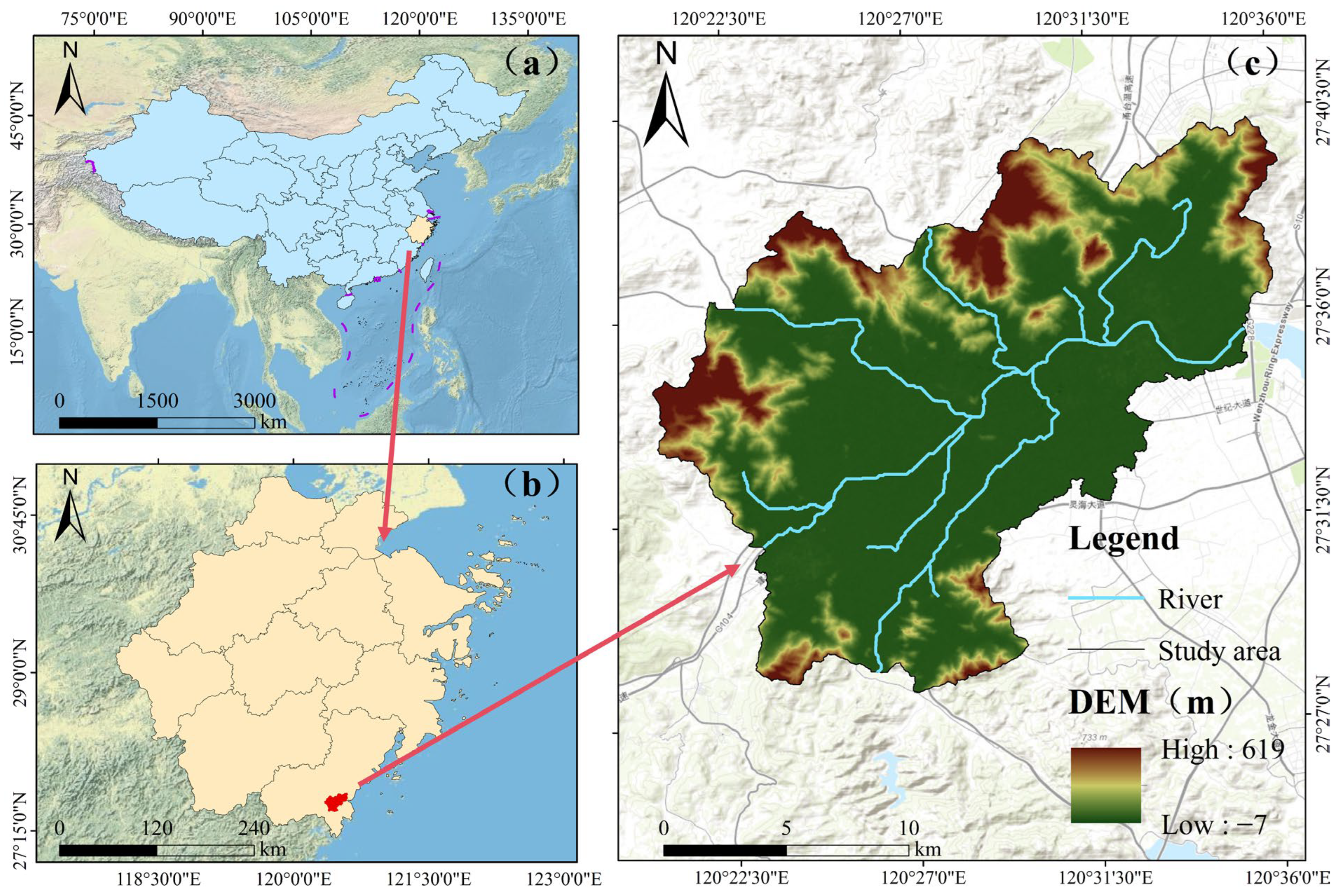
The study area is situated on the west coast of the Pacific Ocean, within the Aojiang River Basin on the southeastern coast of Zhejiang Province, China (Figure 2). This region is frequently affected by typhoons, the occurrence of which often overlaps with the flood season, making it highly susceptible to secondary disasters such as flash floods, mudslides, landslides, and urban waterlogging. Geographically, the area extends from 120.34° E to 120.60° E in longitude and from 27.46° N to 27.68° N in latitude, covering a total area of 326.11 km². The basin features complex topography, with elevations ranging from −7 m to 619 m, encompassing both low-lying plains and steep mountainous hills. The western and northern parts are dominated by high mountains and hilly terrain, where higher elevations prevail and paddy fields are sparsely distributed only in the valleys. This topography causes rapid runoff accumulation after rainfall events, rendering the area prone to mountain floods. In contrast, the central and southern parts of the basin consist of extensive coastal plains characterized by flat terrain, which host the main urban settlements and agricultural land. The region experiences a subtropical monsoon climate, with an average annual precipitation of approximately 1700 mm. The majority of rainfall occurs during the spring and summer months, from March to September. Moreover, the well-developed river network within the watershed makes it susceptible to frequent flooding.

To ensure transparency and reproducibility of the research, this section details the sources, resolution, and processing procedures of the data used in this study.

Table 1. Data source.

Data Type	Detailed Description and Year	Spatial Resolution	Data Source	Primary Use
Terrain data	DEM (2010)	30 m	METI and NASA jointly developed the ASTER GDEM dataset (https://www.gscloud.cn/)	Core input for the HEC-HMS/HEC-RAS model, used to calculate flow paths, slopes, and confluences
Land Use	Land Use Classification (2010, 2020)	30 m	China Multi-Period Land Use Remote Sensing Monitoring Dataset (CNLUCC) (Resource and Environmental Science and Data Center, Chinese Academy of Sciences https://www.resdc.cn/)	Manning roughness coefficient assignment in the HEC model; Benchmark and validation data for the PLUS model
Meteorological data	Average annual precipitation, average annual temperature (2010)	1 km	China 1 km Monthly Precipitation Dataset (1901–2024) [32] 1-km monthly maximum temperature dataset for China (1901–2024) [33]	One of the driving factors of the PLUS model, used to predict future land use
Extreme rainfall sequence	Design rainfall (20, 50, and 100-year return period)	Point Data	Local Hydrological Manual Weather Station Recorded Data	Input boundary conditions for the HEC-HMS model, used to generate flood scenarios
Socioeconomic Data	GDP, Population Density (2010)	1 km	China GDP Spatial Distribution Kilometer Grid Dataset; China Population Spatial Distribution Kilometer Grid Dataset (Chinese Academy of Sciences Resource and Environment Science and Data Center https://www.resdc.cn/)	Direct Vulnerability Indicators (reflecting exposure and sensitivity); PLUS Model Driving Factors
Infrastructure Data	Building coverage, Hospital distance, Hydrological station density, Cultivated land coverage (2020)	Vector/1 km	OpenStreetMap, Zhejiang Provincial Department of Water Resources	Direct Vulnerability Indicators (reflecting exposure, coping capacity, and resilience)
Soil Data	Soil Type (2010, 2020)	1 km	Spatial Distribution Dataset of Soil Types in China (Resource and Environmental Science and Data Center, Chinese Academy of Sciences https://www.resdc.cn/)	Input parameters for calculating SCS curves in the HEC-HMS model
Flood Dynamic Data	Flood Depth at Different Return Periods (2020, 2030)	12.5 m	Simulation Output from Coupled HEC-HMS/HEC-RAS Models	Core Direct Vulnerability Indicator, Quantitatively Characterizing Flood Disaster Severity

summarizes the detailed information for all data. The data in this study can be broadly categorized into two types based on their fundamental purpose within this framework: model inputs and driving data, which are used to drive and calibrate the physical process models we rely on (such as PLUS, HEC-HMS, HEC-RAS); and vulnerability assessment indicator data, which are variables directly used to calculate the final vulnerability index, reflecting a region’s exposure, sensitivity, and resilience.

2.2. Coupled Hydrological-Hydrodynamic Modeling at Street Scale in Complex Coastal Urban Areas

To investigate flood inundation in coastal watersheds under future land-use and extreme rainfall scenarios, we simulated flood scenarios using a coupled approach integrating the HEC-HMS hydrological model and the HEC-RAS hydrodynamic model. The HEC-HMS (Hydrologic Engineering Center–Hydrographic Modeling System) is a semi-distributed, semi-physical hydrological model developed by the Hydrologic Engineering Center of the U.S. Army Corps of Engineers [34,35,36,37]. As a semi-distributed model, it partitions the computational domain into sub-basins and employs a one-dimensional routing scheme to compute runoff pathways [38]. HEC-RAS (Hydrologic Engineering Center River Analysis System), also developed by the U.S. Army Corps of Engineers [39], is a widely used hydrodynamic analysis system for flood modeling. It incorporates capabilities for one-dimensional steady flow simulation, two-dimensional unsteady flow simulation, sediment transport, and water quality modeling [39], making it suitable for fine-scale simulations of hydrodynamic processes, flood risk mapping, and the reconstruction of flood inundation events [40].

Hydrological models are typically employed to calculate the rainfall-runoff processes within basins, nodes, and sub-basins [41] but generally lack detailed hydraulic calculations. In contrast, hydrodynamic models can simulate flash floods or inundation scenarios with high refinement, providing critical disaster characteristics such as inundation depth, flow velocity, and water surface elevation [42]. Leveraging the respective strengths of these models, the proposed methodology first constructs an initial hydrological model to simulate rainfall-runoff processes and derive hydrographs at various nodes and sub-basins. Subsequently, these hydrological model nodes serve as the boundary conditions for the hydrodynamic model, with their computed flood hydrographs used as direct inputs. This establishes a coupled model system for calculating final simulation results. As illustrated in Figure 3, the models are coupled in an external (out-coupling) configuration. In the schematic, triangles represent river nodes constructed in the hydrological model, pentagons denote sub-basins, and a pentagram indicates the flow outlet of the hydrological model. The blue S1 watershed represents the portion of the domain where the hydrodynamic model is coupled with the hydrological inputs and serves as the focal area for detailed hydrodynamic simulation under these derived boundary conditions.

Hydrological analysis was performed based on a Digital Elevation Model (DEM). DEM is derived from the ASTER GDEM V3 dataset. As the core input for terrain analysis and model construction, its effective accuracy sufficiently meets the requirements for watershed-scale hydrological and hydrodynamic simulations [43]. To ensure hydrological correctness, the standard operating procedure involves preprocessing the raw DEM to eliminate anomalous pits and depressions, thereby safeguarding the continuity of surface runoff flow paths. The initial hydrological model was constructed, and its parameters were calculated and assigned using four key methods: the SCS (Soil Conservation Service) curve number method, the SCS unit hydrograph method, the exponential recession method, and the Muskingum routing method. The hydrological model simulated a total period of 180 min, with a rainfall-runoff output interval of 5 min. Subsurface attributes and Manning’s roughness coefficients (N-values) were assigned based on high-precision DEM and land-use data, as summarized in Figure 3.

2.3. Flood Vulnerability Assessment Based on a Hydrodynamic Model in Current and Future Perspectives (VHCF)

2.3.1. PLUS Model-Based Construction of Scenarios

To compare the impacts of current (2020) and projected future land use scenarios on hydrodynamic processes and vulnerability, we employed the Patch-generating Land Use Simulation (PLUS) model. Developed by the High-Performance Spatial Computational Intelligence Laboratory (HPSCOL), the PLUS model integrates a Land Expansion Analysis Strategy (LEAS) with a Cellular Automata (CA) model based on multi-class stochastic patch seeding (CARS). This framework is designed to simulate land-use changes by capturing the dynamic spatial interactions among economic, ecological, and social systems, thereby providing robust support for policy formulation and advancing sustainable development goals.

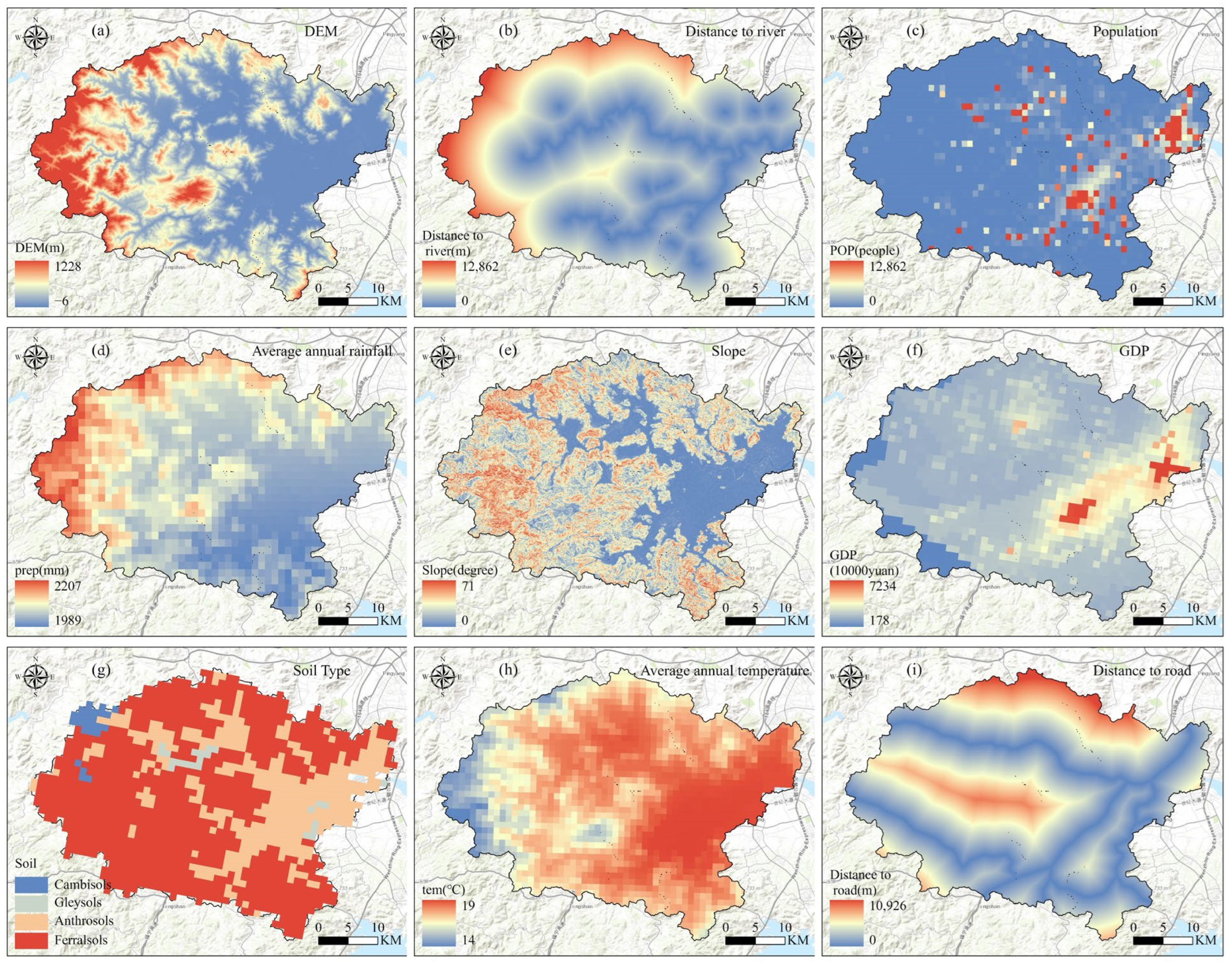
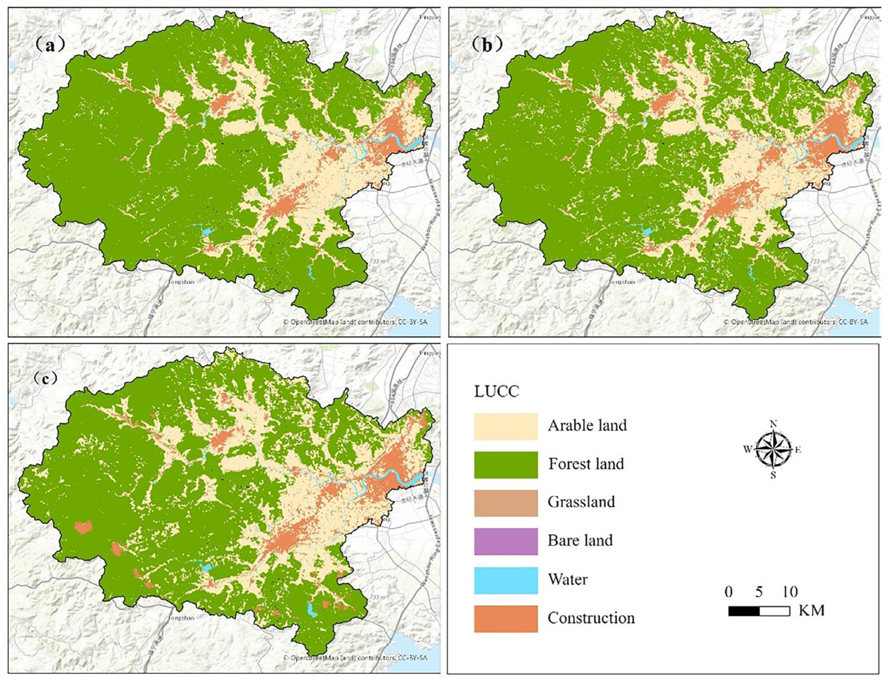
When simulating land use in PLUS, drivers are selected from four major categories: climate, topography, location and transportation, and socioeconomic systems. All driver data were standardized to a consistent geographic coordinate system and grid cell size, then converted into the preprocessed format required by the PLUS model. Detailed driver information is presented in Figure 4. Using 2000 and 2010 land use data as simulation baselines, the PLUS model successfully predicted the 2020 land use status (as shown in Figure 5a,b). The prediction results were validated against actual 2020 data, achieving a Kappa coefficient of 0.81. This indicates extremely high simulation reliability and confirms the model’s applicability for forecasting land use changes in the study area by 2030. The simulated land use for 2030 is shown in Figure 5c.

2.3.2. Vulnerability Assessment of Coupled Hydrologic-Hydrodynamic Processes

Vulnerability was evaluated using an indicator system approach [44]. The inundation depth under different return periods in 2020 and 2030, derived from the coupled hydrological-hydrodynamic simulations, served as a key indicator to reflect the direct threat posed by potential flood events across the region. Adhering to the principles of scientific rigor, representativeness, and practicality [45], and considering the specific context of the study area, additional relevant indicators were incorporated into the vulnerability evaluation framework. A complete list of these indicators is provided in

Table 2. Indicators.

Indicators	Relationship	Resolution	Year
Population density	+	1 km	2020
Percentage of building area	+	\	2020
GDP	−	1 km	2020
Percentage of cultivated land	+	1 km	2020
Density of hydrological stations	−	\	2020
Distance to hospital	+	\	2020
Slope	+	30 m	2020
Inundation water depth 20-year return period	+	12.5 m	2020, 2030
Inundation water depth 50-year return period	+	12.5 m	2020, 2030
Inundation water depth 100-year return period	+	12.5 m	2020, 2030

, where the positive or negative relationship (cardinality) assigned to each indicator was determined based on the established theoretical framework of flood vulnerability and the intrinsic nature of each factor. A positive relationship indicates that an increase in the indicator value leads to an increase in vulnerability. Conversely, a negative relationship suggests that an increase in the indicator value reduces vulnerability. Higher values for positively correlated indicators typically signify greater exposure (e.g., more people and assets at risk), heightened sensitivity (e.g., farmland vulnerable to flooding), or reduced access to critical services during disasters (e.g., greater distance from hospitals), all of which exacerbate vulnerability. Negatively correlated indicators include GDP and the density of hydrological stations. Higher GDP generally signifies stronger disaster prevention, mitigation, and post-disaster economic recovery capabilities. Higher hydrological station density enhances monitoring and early warning capabilities, thereby reducing vulnerability.

Principal Component Analysis (PCA) was employed to determine the weights of each indicator within the evaluation system. Before PCA, all indicator data were normalized. The suitability of the data for PCA was confirmed using the Kaiser-Meyer-Olkin (KMO) test and Bartlett’s test of sphericity. The KMO test measures sampling adequacy, reflecting the proportion of variance among variables that may be attributable to common variance. A value closer to 1.0 indicates greater suitability for PCA. Bartlett’s Sphericity Test is used to examine the correlation between variables. When the significance level (p-value) is less than 0.01, the data is suitable for PCA. After passing the test, principal components with eigenvalues greater than 1 are retained, and weights are assigned based on the percentage of total variance they explain. The weight of each indicator within a principal component was then calculated as the square of its rotated factor loading relative to the sum of squared loadings in that component, ultimately yielding the final weight for each indicator [46]. Once the weights were established, the overall vulnerability values for both current and future scenarios were computed using an indicator aggregation formula (Equation (1)), and corresponding vulnerability maps were generated.

$$V_i=\sum _{i=1}^n{W}_i\ast {In}_i$$

(1)

2.4. VHCF-Based Allocation of Funds for Pre-Disaster Preparedness

2.4.1. Prioritization of Areas to Be Supported and Determination of Benefit Coefficients

Areas characterized by high vulnerability typically experience greater property damage and casualties during flood events, thus requiring focused attention in disaster prevention and mitigation planning [47]. Conversely, areas with low vulnerability are either less prone to flooding or possess higher inherent flood protection capacity, resulting in a lower demand for disaster prevention resources [48]. Consequently, regions were classified based on an integrated assessment of their current and future vulnerability levels. Areas identified as having medium or higher vulnerability were designated as priority zones for financial support.

The primary objective of pre-disaster investment is to enhance local flood prevention capacity and mitigate the negative impacts of flood events. In this model, disaster prevention measures serve as a quantitative proxy to assess the benefits of invested funds, without prescribing specific measures. These benefits are quantified by the reduction in current and future vulnerability values achieved through the investment. A hierarchical approach was adopted to quantify benefit coefficients, acknowledging that areas with different vulnerability levels require distinct levels of resource allocation for effective disaster prevention. As the historical frequency and intensity of hazards in a region influence the development of flood protection infrastructure, the potential benefits of these measures were characterized by quantifying their relevance using a Geodetector [49].

2.4.2. VHCF-Based Model for Allocating Pre-Disaster Disaster Prevention Funds

To maximize the benefits of sustainable pre-disaster funding, a disaster fund allocation model based on the VHCF (designated VHCF-FAOM) was developed. This model builds upon the foundational FAOM [27] and SO-FAOM [28] models. While FAOM and SO-FAOM focus on allocation under current scenarios, VHCF-FAOM incorporates the results of coupled hydrological–hydrodynamic vulnerability assessments, integrating future flood scenarios into the decision-making process. The model construction involves the following steps. First, a base objective function is formulated to allocate funds based on current vulnerability, aiming to minimize the overall regional vulnerability value and reduce the number of areas classified as extremely vulnerable. To ensure the long-term benefit of allocations, these two base objectives are incorporated into a penalty function. This function penalizes investments in areas where future vulnerability (after ten years) is projected to exceed the current level, as well as investments in areas that remain extremely vulnerable. By combining the base objective function and the penalty function, two comprehensive objective functions are created to guide the optimization process, effectively balancing the mitigation of current and future vulnerability to achieve optimal overall efficiency. Finally, constraints are applied to ensure that the total allocated funds do not exceed the total planned budget. The specific construction process is detailed below:

Comprehensive objective function 1:

$$x_{ij}={\displaystyle \frac{P_{ij}}{I_j}}$$

(2)

$$X_{ij}={\displaystyle \frac{x_{ij}-x_{ijmin}}{x_{ijmax}-x_{ijmin}}}$$

(3)

$${DV}_i=\sum _{j=1}^k{X}_{ij}\ast w_{nj}\ast W_j$$

(4)

$${PV}_i=V_i-{DV}_i$$

(5)

$${PV}_i^{\left(10\right)}=V_i^{\left(10\right)}-{DV}_i$$

(6)

$$f_1=\sum _{i=1}^n{PV}_i$$

(7)

$$P_1=\lambda \sum _{i=1}^n{PV}_i^{\left(10\right)}\left({PV}_i^{\left(10\right)}>{PV}_i\right)$$

(8)

$$F_1=\mathit{min}\left(f_1+P_1\right)$$

(9)

where $P_{ij}$ is the amount of money invested in each measure in each unit; $I_j$ is the cost of the measure; $x_{ij}$ is the number of each measure in each unit; $X_{ij}$ is the normalized value of $x_{ij}$; $w_{nj}$ is the benefit coefficient of the $j$th measure in the $n$th priority support level region; $W_j$ is the weight of the corresponding indicator of the $j$th measure; ${DV}_i$ is the vulnerability value that will be reduced after the investment of money; $V_i$ and $V_i^{\left(10\right)}$ are the current and future vulnerability values of the $i$th unit before investing funds; ${PV}_i$ and ${PV}_i^{\left(10\right)}$ are the current and future vulnerability values after investing funds; $\lambda$ is the penalty coefficient; $f_1$ is the first basic objective function; $P_1$ is the penalty function; $F_1$ is the first comprehensive objective function.

Composite objective function 2:

$$f_2=\sum _{i=1}^{n}NUM\left({PV}_i>V_H\right)$$

(10)

$$P_2=\lambda \sum _{i=1}^{n}NUM\left({PV}_i^{\left(10\right)}>V_H\right)$$

(11)

$$F_2=\min \left(f_2+P_2\right)$$

(12)

where $V_H$ is the extreme vulnerability region threshold, higher than the high vulnerability region is considered as the extreme vulnerability region. $f_2$ is the second base objective function; $P_2$ is the corresponding penalization function; and $F_2$ 2 is the second integrated objective function.

Constraints:

$$P=\sum _{i=1}^n \sum _{i=1}^k P_{ij}$$

(13)

where $P_{ij}$ is the $j$th measure input funding in the $i$th unit; $P$ is the total amount of planned input funding.

After establishing the objective functions and constraints, the model is solved using the Nondominated Sorting Genetic Algorithm II (NSGA-II). NSGA-II is designed for multi-objective optimization and combines nondominated sorting with crowding distance computation and an efficient fast-sorting operator to achieve effective Pareto optimization [50]. Furthermore, NSGA-II helps prevent convergence to local optima by maintaining population diversity through its nondominated sorting and crowding distance mechanisms, ultimately yielding a set of Pareto-optimal solutions [51]. Based on the optimal solution set, the optimal solution is identified using TOPSIS. TOPSIS (Technique for Order Preference by Similarity to Ideal Solution) is a multi-attribute decision analysis method that ranks alternatives by comparing their distances to the ideal solution and negative ideal solution and selects the solution that is closest to the ideal solution [20]. Technique for Order Preference by Similarity to Ideal Solution [52,53]. The specific solution method is as follows:

$$r_{ij}={\displaystyle \frac{x_{ij}}{\sqrt{{\sum }_{i=1}^m{x}_{ij}^2}}}$$

(14)

$$D_i^{+}=\sqrt{\sum _{j=1}^m {\left(r_j^{+}-r_{ij}\right)}^2 }$$

(15)

$$D_i^{-}=\sqrt{\sum _{j=1}^m {\left(z_j^{-}-z_{ij}\right)}^2}$$

(16)

$$C_i={\displaystyle \frac{D_i^{-}}{D_i^{+}+D_i^{-}}}$$

(17)

where $x_{ij}$ is the score of the $i$th alternative on the $j$th objective; $r_{ij}$ is the normalized value of the score of the $i$th alternative on the $j$th objective; $D_i^{+}$ is the distance of the $i$th alternative from the positive ideal solution; $D_i^{-}$ is the distance of the $i$th alternative from the negative ideal solution; $C_i$ is the relative proximity of the $i$th alternative, and the maximum value of the relative proximity is the optimal alternative.

3. Results

3.1. Coupled Simulated Flooding Results

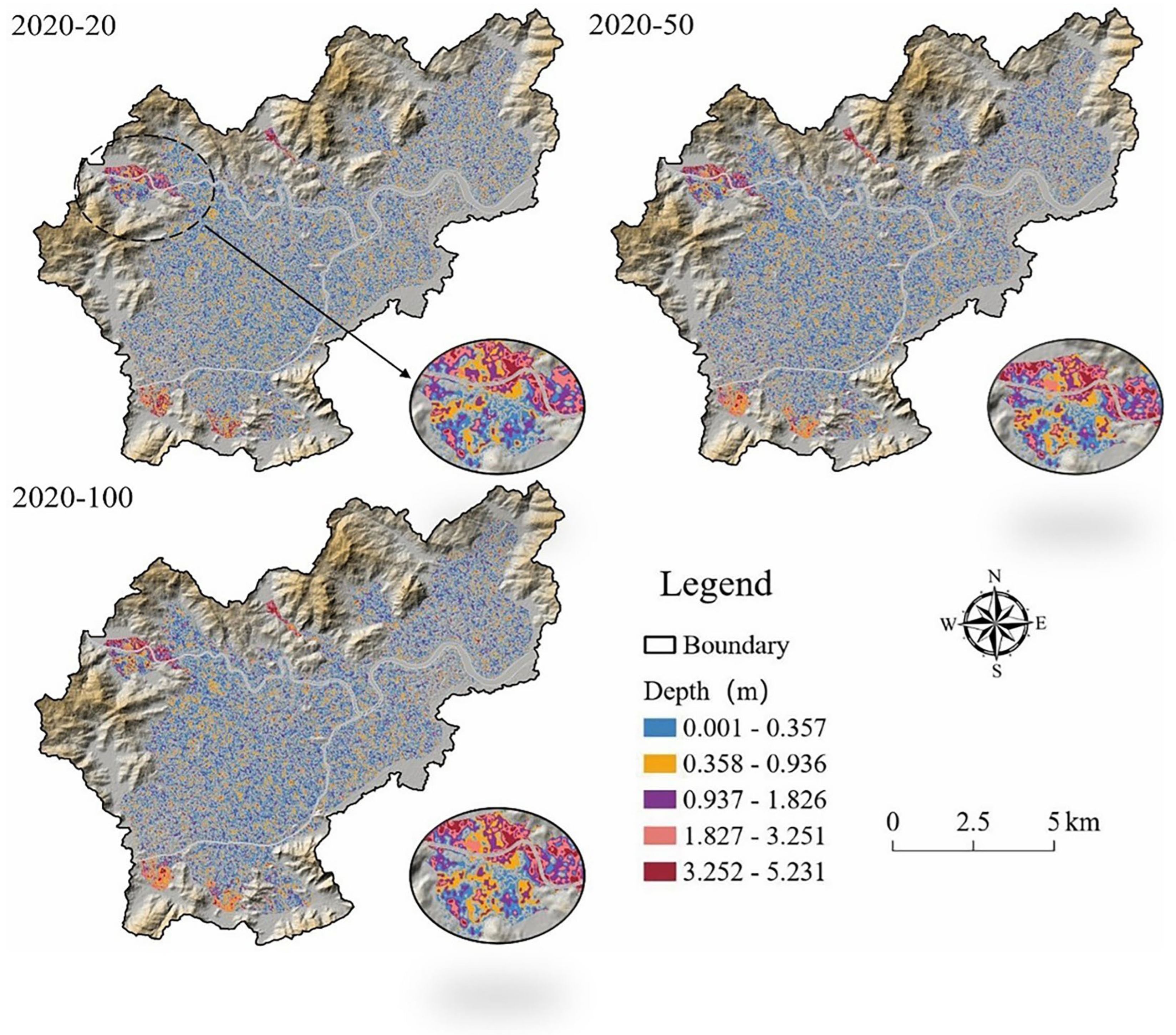
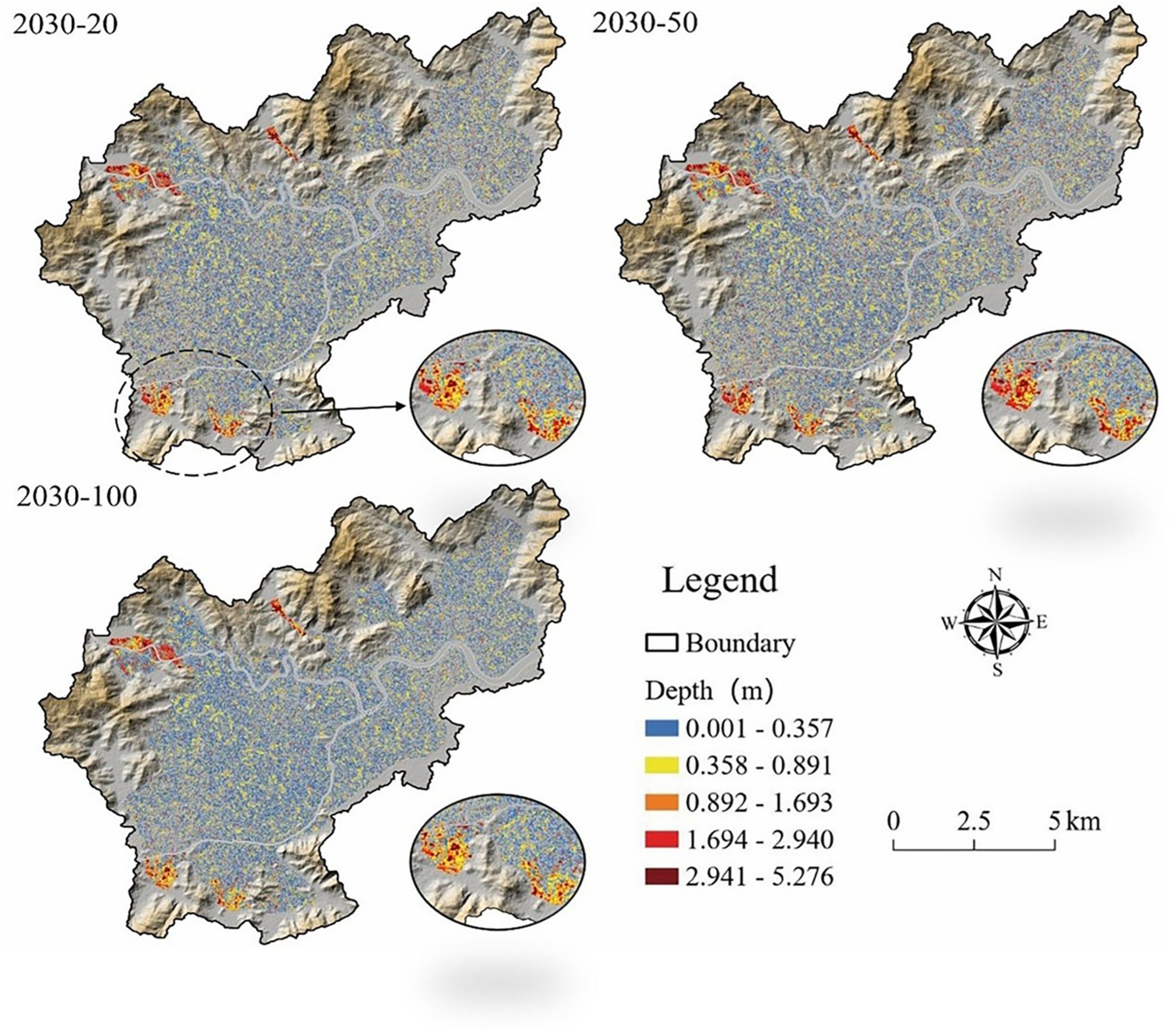
AS illustrated in Figure 6 and Figure 7, the maximum inundation extents under extreme rainfall scenarios for 2020 and 2030 reveal that flooded areas are predominantly located in the flatter parts of the watersheds, mainly covering cultivated and built-up land. Although the overall inundation patterns for 2020 and 2030 do not differ significantly, a more noticeable variation is observed around the coupling nodes, as highlighted in the figures. In both years, the maximum inundation depth exceeds 5 m: specifically, 5.231 m in 2020 and 5.276 m in 2030. A deeper analysis of inundation depths shows that, under the same land use scenario (e.g., 2020), flood severity increases with longer rainfall return periods. The largest inundation depth and extent are observed under the 100-year return period, with a similar trend in 2030. For the 2020 land use scenario, the total inundated areas are 78.45 km² (20-year return period), 81.24 km² (50-year return period), and 83.14 km² (100-year return period). These areas are mostly concentrated in low-lying regions such as riverine zones and floodplains (see Figure 6 and Figure 7). In 2030, the inundated areas are slightly larger: 78.49 km² (20-year), 81.29 km² (50-year), and 83.24 km² (100-year). The spatial distribution also shifts slightly, with increased flooding in newly urbanized zones and along expanded river channels. Compared to 2020, the increases in inundated areas across the three return periods are 0.035 km², 0.05 km², and 0.1 km², respectively, indicating a relatively minor overall change. This increase is more evident near riverbanks and floodplains, which are particularly sensitive to rainfall intensity.

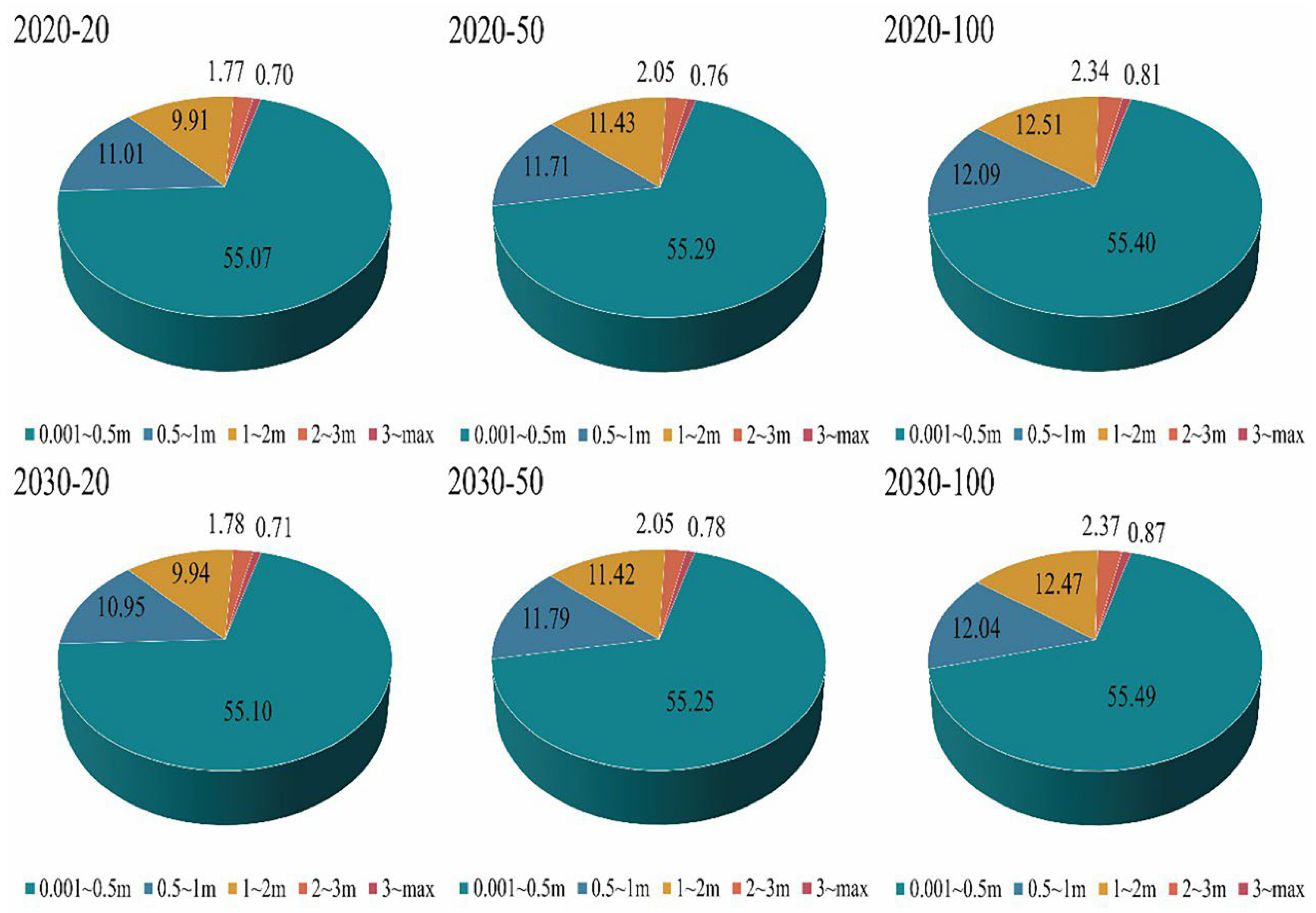
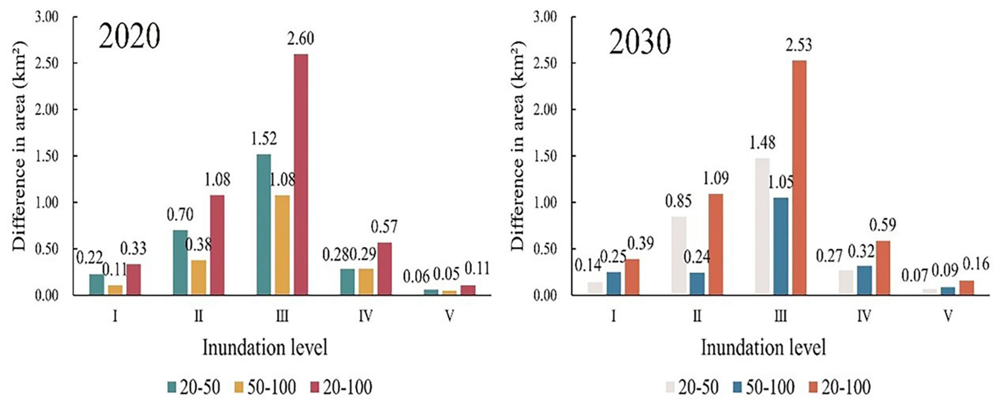
To elaborate on the danger of flooding in more detail, this experiment divides the flood inundation depth into five grades, which are 0.001~0.5 m, 0.5~1 m, 1~2 m, 2~3 m, and 3 m or more, and expresses the degree of its danger by Ⅰ, Ⅱ, Ⅲ, Ⅳ, and V. As shown in Figure 8 and Figure 9, across all simulation scenarios, Grade I inundation (depth < 0.5 m) covers the largest area—approximately 70% of the total flooded area. The extent of each inundation class increases with longer return periods, with areas of depth > 3 m (Grade V) being the smallest. Notably, the increases in Grades I and V areas are minimal, while more substantial growth is observed in Grades II, III, and IV. Among these, Grade III shows the most significant change. For instance, under 2020 land use conditions, the Grade III area increases by about 1.52 km² when moving from a 20-year to a 50-year return period, and by another 1.08 km² from a 50-year to a 100-year return period. These results confirm that, under the same land use scenario, both the total inundated area and flood severity increase with the rainfall return period, reflecting a trend of more severe flooding under higher rainfall intensities. However, the influence of land use change on flood risk—whether measured by total inundated area or the distribution across inundation classes—is relatively small compared to the effect of rainfall intensity (return period).

3.2. VHCF

The KMO test value for vulnerability assessment in the current and future perspectives of coupled hydrological and hydrodynamic processes was 0.71 (p < 0.001), indicating high significance for PCA. The total variance explained by PCA for the indicator data from both the current and future perspectives was 76.82% (

Table A1. Total variance explained by indicators in 2020.

Component	Eigenvalues			Extraction Sums of Squared Loadings			Rotation Sums of Squared Loadings
	λ	% of Variance	Cumulative %	λ	% of Variance	Cumulative %	λ	% of Variance	Cumulative %
1	3.563	35.627	35.627	3.563	35.627	35.627	3.059	30.593	30.593
2	1.937	19.367	54.995	1.937	19.367	54.995	2.048	20.479	51.072
3	1.157	11.567	66.562	1.157	11.567	66.562	1.484	14.843	65.915
4	1.026	10.259	76.821	1.026	10.259	76.821	1.091	10.906	76.821
5	0.99	9.901	86.721
6	0.581	5.807	92.529
7	0.422	4.222	96.751
8	0.311	3.112	99.863
9	0.011	0.113	99.975
10	0.002	0.025	100

) and 76.80% (

Table A2. Total variance explained by indicators in 2030.

Component	Eigenvalues			Extraction Sums of Squared Loadings			Rotation Sums of Squared Loadings
	λ	% of Variance	Cumulative %	λ	% of Variance	Cumulative %	λ	% of Variance	Cumulative %
1	3.557	35.574	35.574	3.557	35.574	35.574	3.057	30.566	30.566
2	1.938	19.384	54.958	1.938	19.384	54.958	2.048	20.477	51.043
3	1.158	11.582	66.54	1.158	11.582	66.54	1.485	14.854	65.897
4	1.027	10.269	76.809	1.027	10.269	76.809	1.091	10.912	76.809
5	0.99	9.903	86.712
6	0.581	5.809	92.521
7	0.422	4.222	96.744
8	0.311	3.112	99.856
9	0.012	0.118	99.974
10	0.003	0.026	100

), respectively. The extracted principal components were able to describe the majority of the data. By combining the variance percentages of each principal component with the rotated factor loadings of the indicators (

Table A3. Rotated factor loadings for 2020 indicators.

Indicators	Extracted Components
	PC1	PC2	PC3	PC4
Inundation water depth 50-year return period	0.981
Inundation water depth 20-year return period	0.98
Inundation water depth 100-year return period	0.979
Population density		0.842
Percentage of building area		0.777
GDP		0.710
Percentage of cultivated land			0.885
Slope			0.772
Density of hydrological stations				0.792
Distance to hospital				0.493

and

Table A4. Table A3 Rotated factor loadings for 2030 indicators.

Indicators	Extracted Components
	PC1	PC2	PC3	PC4
Inundation water depth 50-year return period	0.982
Inundation water depth 20-year return period	0.980
Inundation water depth 100-year return period	0.979
Population density		0.842
Percentage of building area		0.777
GDP		0.709
Percentage of cultivated land			0.885
Slope			0.773
Density of hydrological stations				0.797
Distance to hospital				0.481

), the weights for each indicator were determined, as shown in

Table 3. Indicator weights.

Indicators	Weights (2020)	Weights (2030)
Population density	0.098	0.099
Percentage of building area	0.084	0.084
GDP	0.07	0.07
Percentage of cultivated land	0.086	0.085
Slope	0.065	0.065
Density of hydrological stations	0.096	0.098
Distance to hospital	0.037	0.036
Inundation water depth 20-year return period	0.155	0.154
Inundation water depth 50-year return period	0.155	0.155
Inundation water depth 100-year return period	0.154	0.154

.

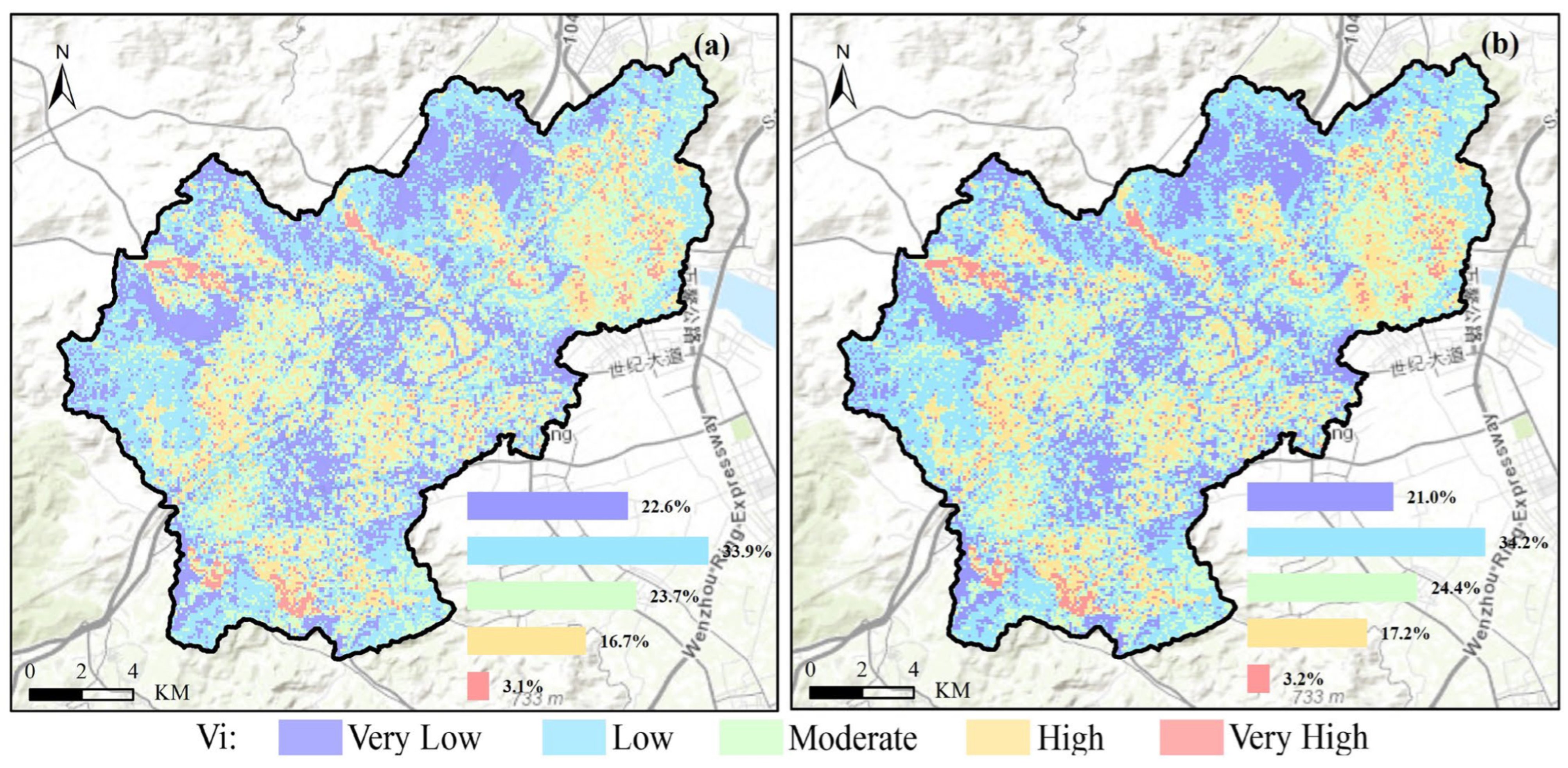
Figure 10 presents the spatial distribution of vulnerability assessed under current (2020) and future (2030) coupled hydrological–hydrodynamic scenarios. In both periods, very high vulnerability areas are predominantly concentrated in urban zones along the river corridors, especially in the southern, northwestern, and northern parts of the study area, with scattered occurrences in the northeast. High vulnerability areas are also mainly clustered in urban settings, while medium vulnerability areas are largely urban with sporadic patches in rural or mountainous regions. In contrast, low and very low vulnerability areas are primarily situated in the northern and western mountainous regions. A comparison of vulnerability statistics between 2020 and 2030 reveals an overall increasing trend in vulnerability. The proportion of very low vulnerability areas decreased from 22.6% to 21.0%, while all other categories showed an increase: low vulnerability areas rose from 33.9% to 34.2%, medium vulnerability from 23.7% to 24.4%, high vulnerability from 16.7% to 17.2%, and very high vulnerability from 3.1% to 3.2%.

3.3. Optimization of Disaster Prevention Funds-Based on VHCF

3.3.1. Prioritized Support Areas and Benefit Factors for Coupled VHCFs

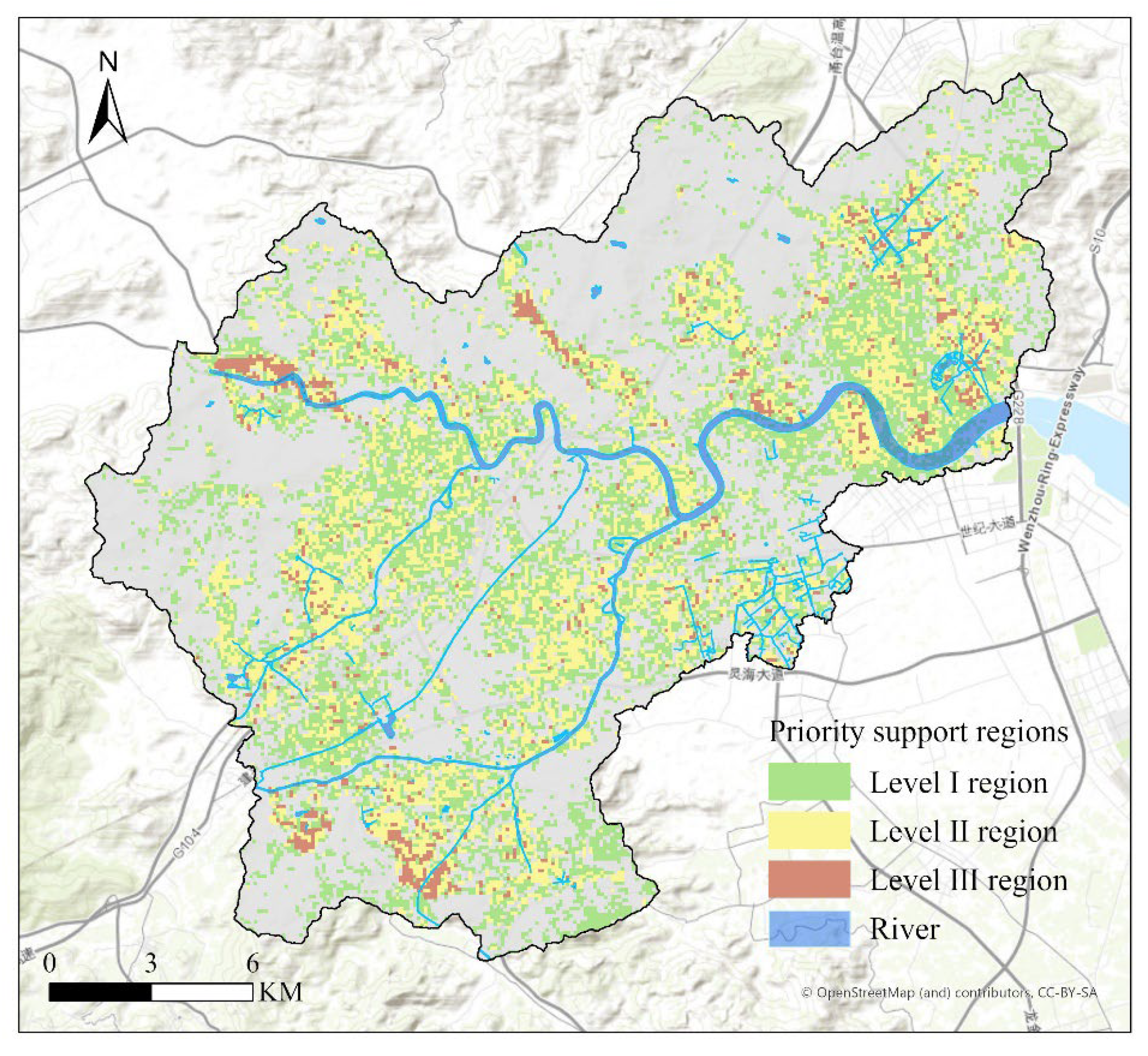
Based on the vulnerability assessment results for both current and future scenarios, areas rated higher than medium vulnerability were identified as priority zones for support. These priority areas were further divided into three levels according to their vulnerability degree, ensuring that regions with extreme vulnerability receive precedence in funding allocation. As illustrated in Figure 11, the prioritized zones are largely concentrated in densely populated and flood-prone locations, such as urban centers and areas adjacent to rivers.

Disaster prevention measures were used as tools to quantify the benefits of the investments. The selection of these measures was aligned with predefined indicators to ensure that benefits could be effectively measured. For practicality and to facilitate visualization of the implementation process, three types of measures were chosen based on the evaluation indicators: hydrological stations, small emergency relief stations, and the construction of high-standard farmland. Among these, the establishment of hydrological stations enhances real-time water level monitoring and early warning capabilities, allowing timely flood alerts and reducing potential losses. The setup of small emergency relief stations enables rapid rescue and medical aid after flooding, improving the accessibility of relief services in certain areas and reducing the risk of casualties. Moreover, high-standard farmland generally includes features such as drainage ditches and flood storage areas, which mitigate flood impact by slowing water flow. The benefits of these disaster prevention measures were quantified hierarchically using Geodetector, with the benefit coefficients presented in

Table 4. Benefit coefficient.

Levels of Social Vulnerability	Measures
	Hydrological Monitoring Stations	Small-Scale Emergency Relief Stations	High Standard Farmland
Level I region	0.106	0.042	0.033
Level II region	0.209	0.098	0.075
Level III region	0.318	0.166	0.129

. The higher the priority level of the support area, the greater the benefits generated by the measures. At the same priority level, hydrological stations delivered greater benefits than the other two measures, likely because pre-disaster warnings are the most direct and impactful.

3.3.2. Results of the Allocation of Funds to the Coupled VHCF

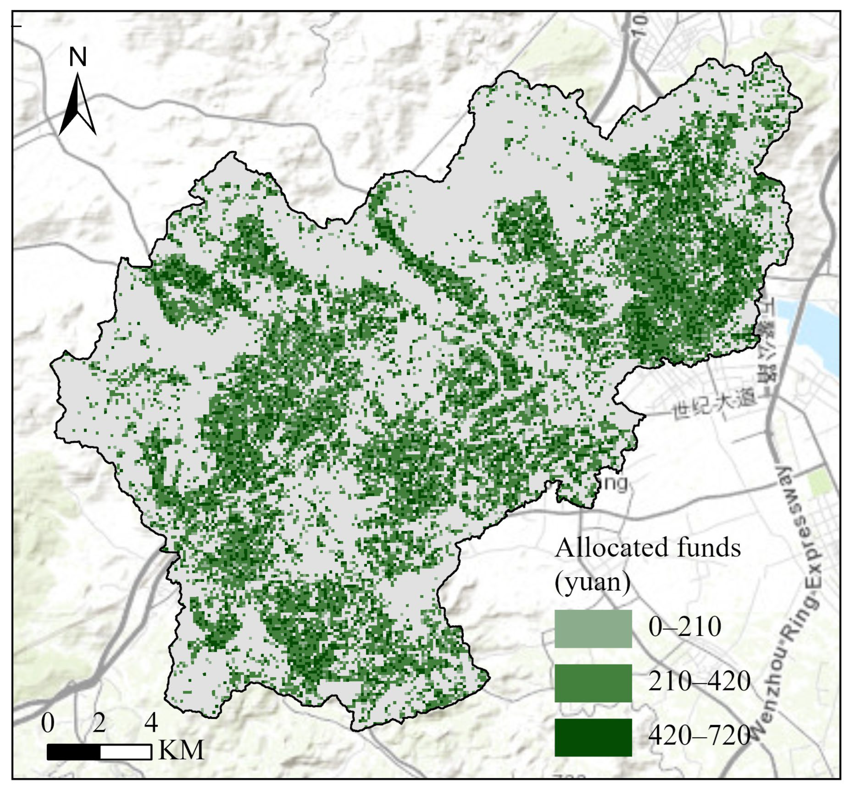
The specific input conditions for constructing the VHCF-FAOM model were as follows: the total input capital was set at 5 million yuan; the initial population size was 1000; the number of iterations was 1000; the crossover was simulated using the binary crossover operator, with a crossover probability of 85% and a distribution index of 20; and the mutation probability was 15%, with a distribution index of 20. The VHCF-FAOM model produced two solutions, each of which was part of the Pareto optimal solution set. As shown in

Table 5. TOPSIS identifies the optimal fund’s allocation scheme.

Pareto Optimal Set	f1	f2	Relative Proximity
Case 1	5606.04	98	0.99
Case 2	5606.45	97	0.01

, the two solutions achieved the minimum values of 5606.04 and 5606.45 for the first comprehensive objective function, and 98 and 97 for the second comprehensive objective function. The relative proximity of the two solutions was calculated using TOPSIS, yielding values of 0.99 and 0.01, with solution one being selected as the optimal fund allocation solution. To facilitate the visualization of the fund allocation, the results were divided into three levels, as shown in Figure 12. The highest allocated fund was 715 yuan, while the lowest was only 16 yuan. In most regions, the allocated funds ranged between 210 yuan and 420 yuan. The number of funds allocated at the lowest and highest levels was roughly equal, with the number of funds in the highest range being slightly larger than in the lowest range. The overall spatial distribution of funding followed a similar pattern to the vulnerability, with the highest percentage of funding concentrated in the southern, northwestern, and northern parts of the study area.

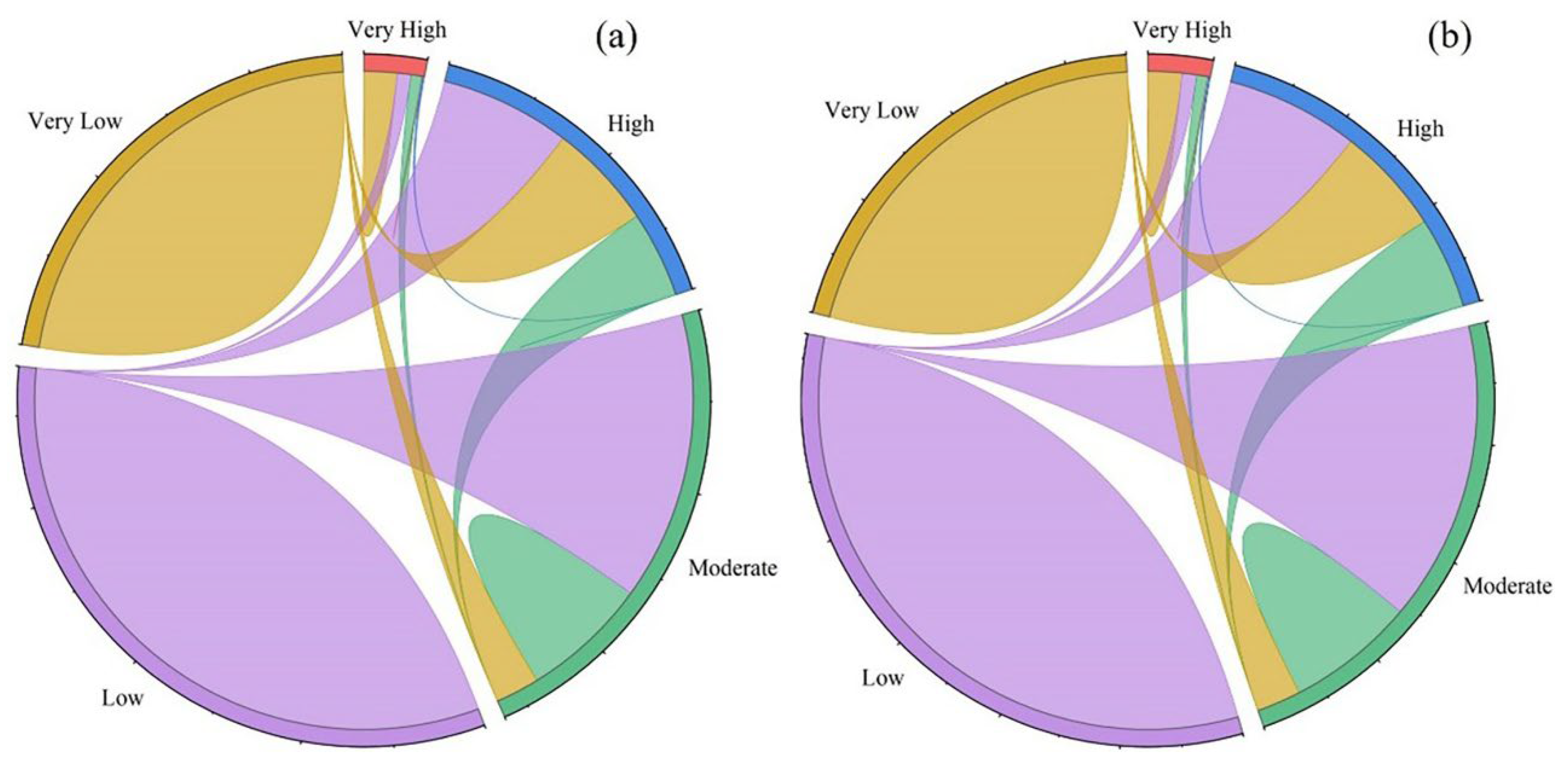
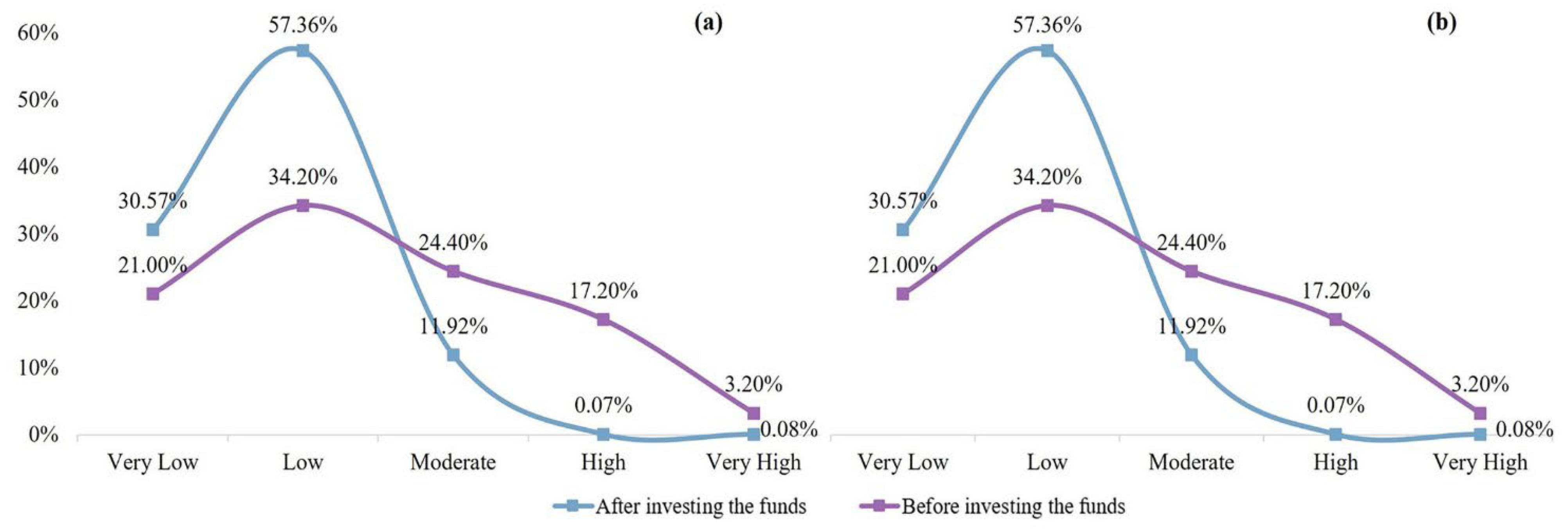
After the investment of funds, the flood control capacity in the study area was improved to varying degrees, which was reflected in changes in the vulnerability levels. The relationship between the number of vulnerability classes in the study area is illustrated in Figure 13 (the color of the string corresponds to the color of the target node), where Figure 13a shows the change in the number of vulnerability classes in 2020 and Figure 13b depicts the change in 2030 following the investment. Following the allocation of funds, the trend in vulnerability ratings shifted in most regions toward low vulnerability. The most significant shift occurred from medium to low vulnerability, followed by areas of high vulnerability transitioning to low vulnerability. For the extreme vulnerability areas, most cells in the very high and high vulnerability areas were converted to very low, low, and medium vulnerability areas, while a few cells in the very high vulnerability areas shifted to high vulnerability areas. Before and after the investment, the number of regions at each vulnerability level was shown in Figure 14, where Figure 14a,b displays the number of regions with different vulnerability levels in 2020 and 2030, respectively. After the fund input, the percentage of low-vulnerability regions increased to 56.29% and 57.36%, respectively. The number of extreme vulnerability areas was significantly reduced. Except for the very high vulnerability areas in 2030, which accounted for 0.08%, the rest of the extreme vulnerability areas accounted for 0.07%, with only a small number of areas maintaining extreme and high vulnerability. The majority of regions had experienced a decrease in vulnerability rank, with the number of moderate vulnerability areas also declining significantly, reaching half of what it was before the fund investment.

4. Discussion

4.1. Spatial Heterogeneity in VHCF

By integrating hydrological and hydrodynamic processes, the spatial characteristics of vulnerability areas were analyzed for 2020 and 2030, enabling a comprehensive assessment of flood vulnerability from both current and future perspectives. As illustrated in Figure 10, areas of very high vulnerability are predominantly concentrated in riverine towns, whereas high-vulnerability areas are largely distributed in more densely urbanized regions. Specifically, in 2020, very high vulnerability areas were mainly located in riverine towns and low-lying areas in the southern, northwestern, and northern parts of the study area (Figure 4). The heightened vulnerability in these riverine zones is attributed to their lower topography, coupled with higher population densities and building intensities, which amplify their exposure to flood hazards and lead to a concentration of flood risk [54] (Figure 6 and Figure 7). The increase in impervious surfaces associated with urbanization further exacerbates floodwater accumulation and propagation, significantly intensifying intra-urban vulnerability [55]. In contrast, areas of low and very low vulnerability are primarily situated in the northern and western mountainous regions. These areas experience less flood impact due to their higher elevation, complex topography, sparse building distribution, and low population density.

Both urbanization and climate change are projected to exacerbate flood risk, consequently increasing the proportion of vulnerable areas [56]. Urbanization contributes to flood risk by expanding impervious surfaces, which in turn increases surface runoff [57]. Simultaneously, climate change is expected to increase the frequency and intensity of extreme precipitation events, further elevating the flood risk in these regions [58]. Changes in indicator weights, as shown in Table 3, reflect the dual impacts of urbanization and climate change. For instance, the weight of population density increased from 0.098 to 0.099, and the weight of hydrological station density rose from 0.096 to 0.098. Conversely, the weight of the percentage of arable land decreased from 0.086 to 0.085. The comprehensive analysis (Figure 10) indicates that the proportional distribution of highly vulnerable areas is projected to increase by 2030 compared to 2020, suggesting that flood vulnerability will continue to escalate with ongoing urbanization and climate change.

The VHCF, by coupling hydrologic and hydrodynamic processes, enables accurate simulation of flood scenarios under different return periods. In the vulnerability assessment, this method quantifies flood process indicators (e.g., water depth in each evaluation cell under various return periods) for each computational cell through numerical simulation. This approach effectively quantifies the impacts of the flood process on the attributes of the disaster-bearing body, enabling a comprehensive evaluation of flood vulnerability at a refined scale. Furthermore, the VHCF, incorporating both current and future perspectives, reveals the potential variability of floods under future scenarios. This provides a more scientific basis for subsequent flood management strategies and the allocation of disaster prevention funds.

4.2. Effectiveness of VHCF-FAOM in Integrating Future Perspectives

In flood disaster management, the precise allocation of disaster prevention resources is crucial for reducing disaster losses and enhancing urban resilience. Vulnerability assessment, which integrates various factors such as the distribution of disaster-bearing bodies, infrastructure, and environmental conditions, provides a comprehensive evaluation of regional susceptibility to flood hazards [59]. Allocating funds based on vulnerability assessment results enables the precise identification of highly vulnerable groups or areas. This ensures that resources are directed to regions requiring prioritized support, thereby optimizing resource utilization and minimizing waste. However, traditional vulnerability assessment methods may fail to comprehensively identify potential flood risks in the context of frequent climate change and extreme weather events. In contrast, vulnerability assessment based on coupled hydrological and hydrodynamic processes can dynamically simulate flooding and evaluate the flood status of different areas under various scenarios, thereby identifying flood-prone areas in a more refined manner [60]. This facilitates more targeted fund allocation, improving the sustainability of urban disaster prevention capacity.

Building upon the coupled hydrological–hydrodynamic vulnerability assessment, the VHCF-FAOM incorporates a future perspective to address rapidly changing climate conditions and future disaster risks, enabling the long-term and accurate allocation of funds. The VHCF-FAOM initially allocates disaster prevention funds based on current vulnerability assessment results and applies a control function to areas that fail to meet future targets. This ensures that the allocated funds achieve the minimization of vulnerability from both current and future perspectives. Consequently, the funding strategy not only addresses current flood protection needs but also maximizes the area’s resilience to future flood hazards. Simulation results demonstrate that the final fund allocation reduces overall vulnerability and decreases the number of extremely vulnerable areas from both current and future perspectives. As shown in Figure 14, after fund allocation, the proportion of areas classified as having low and very low vulnerability reached 88.29% and 87.93% for the current and future perspectives, respectively. This indicates that most areas have developed certain flood prevention capacities for both present and future scenarios. Additionally, the VHCF-FAOM significantly reduced the number of extremely vulnerable areas under both perspectives. By integrating current and future considerations in fund allocation, resources can be directed towards the improvement and construction of critical facilities in high-vulnerability areas, enabling long-term disaster prevention deployment before disasters occur. This effectively mitigates losses from both current and future disasters and contributes to efficient flood disaster management.

In the context of rapid climate change, short-term pre-disaster resource planning is increasingly inadequate to address the growing complexity of flooding. Incorporating a future perspective into the allocation of disaster prevention funds aligns with the principles of sustainable development. This approach not only improves fund utilization efficiency, reduces resource waste, and minimizes disaster losses but also promotes long-term planning for disaster prevention and mitigation. As urbanization accelerates, integrating current and future perspectives in disaster prevention fund allocation ensures the sustainable enhancement of urban resilience and plays a critical role in addressing challenges posed by natural disasters.

5. Conclusions

The study analyzed the spatial heterogeneity of flood vulnerability based on social vulnerability to floods (VHCF) combined with hydrodynamic modeling, and explored the changes in vulnerability areas between 2020 and 2030. The results show that the very high vulnerability areas are mainly concentrated in riverine towns, while the high vulnerability areas are mainly distributed in dense urban areas. Specifically, the very high vulnerability areas in 2020 are mainly concentrated in riverine towns and low-lying areas in the southern, northwestern, and northern parts of the study area, which are usually densely populated, with many buildings and fragile infrastructures, and are exposed to a higher risk of flood inundation. With the accelerated urbanization and the impact of climate change, the proportion of high vulnerability areas will increase in 2030, which suggests that the risk of flooding will increase in the future.

A pre-disaster funding allocation model is proposed based on VHCF by combining the vulnerability assessment of hydrological and hydrodynamic processes, aiming to optimize the allocation of disaster prevention resources and maximize the benefits of disaster prevention measures. The results show that the current and future vulnerability assessments can effectively identify highly vulnerable areas and provide a scientific basis for funding allocation. The optimized current and future perspectives account for 88.29% and 87.93% of the number of low and very low vulnerability areas, respectively. By introducing the future perspective, the VHCF-FAOM model not only improves the current flood prevention capacity but also ensures that future disaster prevention resources can effectively respond to changing climate conditions and disaster risks. In conclusion, the integration of current and future perspectives in disaster prevention fund allocation was shown to not only improve the efficiency of fund utilization and avoid wastage of resources but also promote the sustainable enhancement of urban disaster resilience.

However, there are some limitations of this study, mainly in terms of data availability and modeling complexity. Future studies could consider introducing more indicators and higher spatial resolution to provide a more refined reference for funding optimization. A more comprehensive analysis could provide decision-makers with more targeted recommendations to more effectively address the challenges posed by flood hazards.

References

1. Deng, Z.; Wang, Z.; Wu, X.; Lai, C.; Zeng, Z. Strengthened tropical cyclones and higher flood risk under compound effect of climate change and urbanization across China’s Greater Bay Area. Urban Clim. 2022, 44, 101224. [Google Scholar] [CrossRef]
2. Chen, W.; Huang, G.; Zhang, H.; Wang, W. Urban inundation response to rainstorm patterns with a coupled hydrodynamic model: A case study in Haidian Island, China. J. Hydrol. 2018, 564, 1022–1035. [Google Scholar] [CrossRef]
3. Chen, X.; Zhang, H.; Chen, W.; Huang, G. Urbanization and climate change impacts on future flood risk in the Pearl River Delta under shared socioeconomic pathways. Sci. Total Environ. 2021, 762, 143144. [Google Scholar] [CrossRef] [PubMed]
4. Yarveysi, F.; Alipour, A.; Moftakhari, H.; Jafarzadegan, K.; Moradkhani, H. Block-level vulnerability assessment reveals disproportionate impacts of natural hazards across the conterminous United States. Nat. Commun. 2023, 14, 4222. [Google Scholar] [CrossRef]
5. Clark, M.P.; Wilby, R.L.; Gutmann, E.D.; Vano, J.A.; Gangopadhyay, S.; Wood, A.W.; Fowler, H.J.; Prudhomme, C.; Arnold, J.R.; Brekke, L.D. Characterizing Uncertainty of the Hydrologic Impacts of Climate Change. Curr. Clim. Change Rep. 2016, 2, 55–64. [Google Scholar] [CrossRef]
6. Ahmadalipour, A.; Moradkhani, H.; Castelletti, A.; Magliocca, N. Future drought risk in Africa: Integrating vulnerability, climate change, and population growth. Sci. Total Environ. 2019, 662, 672–686. [Google Scholar] [CrossRef]
7. Lyu, H.M.; Sun, W.J.; Shen, S.L.; Arulrajah, A. Flood risk assessment in metro systems of mega-cities using a GIS-based modeling approach. Sci. Total Environ. 2018, 626, 1012–1025. [Google Scholar] [CrossRef]
8. Danumah, J.H.; Odai, S.N.; Saley, B.M.; Szarzynski, J.; Thiel, M.; Kwaku, A.; Kouame, F.K.; Akpa, L.Y. Flood risk assessment and mapping in Abidjan district using multi-criteria analysis (AHP) model and geoinformation techniques, (cote d’ivoire). Geoenviron. Disasters 2016, 3, 10. [Google Scholar] [CrossRef]
9. Huang, G.; Luo, H.; Chen, W.; Pan, J. Scenario Modeling and Risk Assessment of Urban Flooding in Donghaochong Basin, Guangzhou, China. Adv. Water Sci. 2019, 30, 643–652. [Google Scholar] [CrossRef]
10. Cabrera, J.S.; Lee, H.S. Flood risk assessment for Davao Oriental in the Philippines using geographic information system-based multi-criteria analysis and the maximum entropy model. J. Flood Risk Manag. 2020, 13, e12607. [Google Scholar] [CrossRef]
11. Zeleňáková, M.; Gaňová, L.; Purcz, P.; Satrapa, L. Methodology of flood risk assessment from flash floods based on hazard and vulnerability of the river basin. Nat. Hazards 2015, 79, 2055–2071. [Google Scholar] [CrossRef]
12. Rana, I.A.; Routray, J.K. Integrated methodology for flood risk assessment and application in urban communities of Pakistan. Nat. Hazards 2018, 91, 239–266. [Google Scholar] [CrossRef]
13. Meyer, V.; Haase, D.; Scheuer, S. Flood risk assessment in european river basins—Concept, methods, and challenges exemplified at the mulde river. Integr. Environ. Assess. Manag. 2009, 5, 17–26. [Google Scholar] [CrossRef] [PubMed]
14. Wang, Q.; Xiong, J.; Cheng, W.; Cui, X.; Pang, Q.; Liu, J.; Chen, W.; Tang, H.; Song, N. A landslide susceptibility assessment method coupling statistical methods, machine learning models and clustering algorithms. J. Geo-Inf. Sci. 2024, 26, 620–637. [Google Scholar]
15. Yin, D.; Zhang, X.; Cheng, Y.; Jia, H.; Jia, Q.; Yang, Y. Can flood resilience of green-grey-blue system cope with future uncertainty? Water Res. 2023, 242, 120315. [Google Scholar] [CrossRef] [PubMed]
16. Xu, Y.; Yang, Y.; Wang, Z.; Xiong, J.; Yong, Z.; Zhang, X.; Liu, J.; Chen, G.; Zhao, Q.; Hao, J.; et al. Dynamic response of flood risk in urban-township complex to future uncertainty. Int. J. Disaster Risk Reduct. 2024, 114, 104999. [Google Scholar] [CrossRef]
17. Khajehei, S.; Ahmadalipour, A.; Shao, W.; Moradkhani, H. A Place-based Assessment of Flash Flood Hazard and Vulnerability in the Contiguous United States. Sci. Rep. 2020, 10, 448. [Google Scholar] [CrossRef]
18. Kulp, S.A.; Strauss, B.H. New elevation data triple estimates of global vulnerability to sea-level rise and coastal flooding. Nat. Commun. 2019, 10, 4844. [Google Scholar] [CrossRef]
19. Bertsch, R.; Glenis, V.; Kilsby, C. Building level flood exposure analysis using a hydrodynamic model. Environ. Model. Softw. 2022, 156, 105490. [Google Scholar] [CrossRef]
20. Yang, Q.; Wu, W.; Wang, Q.J.; Vaze, J. A 2D hydrodynamic model-based method for efficient flood inundation modelling. J. Hydroinform. 2022, 24, 1004–1019. [Google Scholar] [CrossRef]
21. Yang, W.; Xu, K.; Lian, J.; Bin, L.; Ma, C. Multiple flood vulnerability assessment approach based on fuzzy comprehensive evaluation method and coordinated development degree model. J. Environ. Manag. 2018, 213, 440–450. [Google Scholar] [CrossRef]
22. Karagiorgos, K.; Thaler, T.; Huebl, J.; Maris, F.; Fuchs, S. Multi-vulnerability analysis for flash flood risk management. Nat. Hazards 2016, 82, S63–S87. [Google Scholar] [CrossRef]
23. Ogie, R.I.; Holderness, T.; Dunn, S.; Turpin, E. Assessing the vulnerability of hydrological infrastructure to flood damage in coastal cities of developing nations. Comput. Environ. Urban Syst. 2018, 68, 97–109. [Google Scholar] [CrossRef]
24. Tanir, T.; de Lima, A.d.S.; Coelho, G.d.A.; Uzun, S.; Cassalho, F.; Ferreira, C.M. Assessing the spatiotemporal socioeconomic flood vulnerability of agricultural communities in the Potomac River Watershed. Nat. Hazards 2021, 108, 225–251. [Google Scholar] [CrossRef]
25. Yang, Y.; Guo, H.; Wang, D.; Ke, X.; Li, S.; Huang, S. Flood vulnerability and resilience assessment in China based on super-efficiency DEA and SBM-DEA methods. J. Hydrol. 2021, 600, 126470. [Google Scholar] [CrossRef]
26. Jun, J.H.; Soojun, K.I.M.; Myungjin, L.; Kim, H.S. A Study on Determination of Investment Priority of Flood Control Considering Flood Vulnerability. J. Korean Soc. Hazard Mitig. 2018, 18, 417–429. [Google Scholar] [CrossRef]
27. Yang, W.; Xu, K.; Ma, C.; Lian, J.; Jiang, X.; Zhou, Y.; Bin, L. A novel multi-objective optimization framework to allocate support funds for flash flood reduction based on multiple vulnerability assessment. J. Hydrol. 2021, 603, 127144. [Google Scholar] [CrossRef]
28. Zhong, J.; Yang, Y.; Wang, Z.; Xiong, J.; Xu, Y.; Hao, J.; Ma, Y.; Shen, G.; Yong, Z. Pre-disaster flood prevention funds allocation and benefit analysis considering social vulnerability to enhance urban sustainable flood resilience. Int. J. Disaster Risk Reduct. 2025, 119, 105324. [Google Scholar] [CrossRef]
29. Huang, J.; Yang, Y.; Yang, Y.; Fang, Z.; Wang, H. Risk assessment of urban rainstorm flood disaster based on land use/land cover simulation. Hydrol. Process. 2022, 36, 14771. [Google Scholar] [CrossRef]
30. Shan, X.; Yin, J.; Wang, J. Risk assessment of shanghai extreme flooding under the land use change scenario. Nat. Hazards 2022, 110, 1039–1060. [Google Scholar] [CrossRef]
31. Peiris, M.T.O.V. Assessment of Urban Resilience to Floods: A Spatial Planning Framework for Cities. Sustainability 2024, 16, 9117. [Google Scholar] [CrossRef]
32. Shouzhang, P. 1-km Monthly Precipitation Dataset for China (1901–2024); National Tibetan Plateau Data Center: Beijing, China, 2025. [Google Scholar]
33. Shouzhang, P. 1-km Monthly Maximum Temperature Dataset for China (1901–2024); National Tibetan Plateau Data Center: Beijing, China, 2025. [Google Scholar]
34. Agarwal, D.S.; Bharat, A.; Kjeldsen, T.R.; Adeyeye, K. Assessing Impact of Nature Based Solutions on Peak Flow Using HEC-HMS. Water Resour. Manag. 2024, 38, 1125–1140. [Google Scholar] [CrossRef]
35. Cheng, X.; Ma, X.; Wang, W.; Xiao, Y.; Wang, Q.; Liu, X. Application of HEC-HMS Parameter Regionalization in Small Watershed of Hilly Area. Water Resour. Manag. 2021, 35, 1961–1976. [Google Scholar] [CrossRef]
36. Dariane, A.B.; Javadianzadeh, M.M.; James, L.D. Developing an Efficient Auto-Calibration Algorithm for HEC-HMS Program. Water Resour. Manag. 2016, 30, 1923–1937. [Google Scholar] [CrossRef]
37. Gumindoga, W.; Rwasoka, D.T.; Nhapi, I.; Dube, T. Ungauged runoff simulation in Upper Manyame Catchment, Zimbabwe: Application of the HEC-HMS model. Phys. Chem. Earth Parts A/B/C 2017, 100, 371–382. [Google Scholar] [CrossRef]
38. Jam-Jalloh, S.U.; Liu, J.; Wang, Y.; Liu, Y. Coupling WRF with HEC-HMS and WRF-Hydro for flood forecasting in typical mountainous catchments of northern China. Nat. Hazards Earth Syst. Sci. 2024, 24, 3155–3172. [Google Scholar] [CrossRef]
39. Ezz, H. Integrating GIS and HEC-RAS to model Assiut plateau runoff. Egypt. J. Remote Sens. Space Sci. 2018, 21, 219–227. [Google Scholar] [CrossRef]
40. Peker, İ.B.; Gülbaz, S.; Demir, V.; Orhan, O.; Beden, N. Integration of HEC-RAS and HEC-HMS with GIS in Flood Modeling and Flood Hazard Mapping. Sustainability 2024, 16, 1226. [Google Scholar] [CrossRef]
41. Yuan, W.; Liu, M.; Wan, F. Calculation of Critical Rainfall for Small-Watershed Flash Floods Based on the HEC-HMS Hydrological Model. Water Resour. Manag. 2019, 33, 2555–2575. [Google Scholar] [CrossRef]
42. Wen, J.; Ju, M.; Jia, Z.; Su, L.; Wu, S.; Su, Y.; Liufu, W.; Yin, H. A Computational Tool to Track Sewage Flow Discharge into Rivers Based on Coupled HEC-RAS and DREAM. Water 2024, 16, 51. [Google Scholar] [CrossRef]
43. Xu, C.W.; Yang, J.S.; Wang, L.Y. Application of Remote-Sensing-Based Hydraulic Model and Hydrological Model in Flood Simulation. Sustainability 2022, 14, 8576. [Google Scholar] [CrossRef]
44. Mwalwimba, I.K.; Manda, M.; Ngongondo, C. Measuring vulnerability to assess households resilience to flood risks in Karonga district, Malawi. Nat. Hazards 2024, 120, 6609–6628. [Google Scholar] [CrossRef]
45. Chan, S.W.; Abid, S.K.; Sulaiman, N.; Nazir, U.; Azam, K. A systematic review of the flood vulnerability using geographic information system. Heliyon 2022, 8, e09075. [Google Scholar] [CrossRef] [PubMed]
46. Chakraborty, L.; Rus, H.; Henstra, D.; Thistlethwaite, J.; Scott, D. A place-based socioeconomic status index: Measuring social vulnerability to flood hazards in the context of environmental justice. Int. J. Disaster Risk Reduct. 2020, 43, 101394. [Google Scholar] [CrossRef]
47. Mallick, J.; Salam, R.; Amin, R.; Islam, A.R.M.T.; Islam, A.; Siddik, M.N.A.; Alam, G.M.M. Assessing factors affecting drought, earthquake, and flood risk perception: Empirical evidence from Bangladesh. Nat. Hazards 2022, 112, 1633–1656. [Google Scholar] [CrossRef]
48. Bin, L.; Xu, K.; Pan, H.; Zhuang, Y.; Shen, R. Urban flood risk assessment characterizing the relationship among hazard, exposure, and vulnerability. Environ. Sci. Pollut. Res. 2023, 30, 86463–86477. [Google Scholar] [CrossRef] [PubMed]
49. Welsch, D.M.; Winden, M.W.; Zimmer, D.M. The effect of flood mitigation spending on flood damage: Accounting for dynamic feedback. Ecol. Econ. 2022, 192, 107273. [Google Scholar] [CrossRef]
50. Rabbani, M.; Oladzad-Abbasabady, N.; Akbarian-Saravi, N. Ambulance Routing in Disaster Response Considering Variable Patient Condition: Nsga-Ii and Mopso Algorithms. J. Ind. Manag. Optim. 2022, 18, 1035–1062. [Google Scholar] [CrossRef]
51. Ma, H.; Zhang, Y.; Sun, S.; Liu, T.; Shan, Y. A comprehensive survey on NSGA-II for multi-objective optimization and applications. Artif. Intell. Rev. 2023, 56, 15217–15270. [Google Scholar] [CrossRef]
52. Wang, X. Pre-assessment for ice disaster in Ning-Meng reaches of the Yellow river based on improved TOPSIS under three-parameter interval grey number. Int. J. Disaster Risk Reduct. 2022, 83, 103430. [Google Scholar] [CrossRef]
53. Zavadskas, E.K.; Mardani, A.; Turskis, Z.; Jusoh, A.; Nor, K.M.D. Development of TOPSIS Method to Solve Complicated Decision-Making Problems: An Overview on Developments from 2000 to 2015. Int. J. Inf. Technol. Decis. Mak. 2016, 15, 645–682. [Google Scholar] [CrossRef]
54. Kara, R.; Singh, P. Flood assessment for Lower Godavari basin by using the application of GIS-based analytical hierarchy process. Int. J. Syst. Assur. Eng. Manag. 2024. [Google Scholar] [CrossRef]
55. Erena, S.H.; Worku, H. Urban flood vulnerability assessments: The case of Dire Dawa city, Ethiopia. Nat. Hazards 2019, 97, 495–516. [Google Scholar] [CrossRef]
56. Wang, M.; Fu, X.; Zhang, D.; Chen, F.; Liu, M.; Zhou, S.; Su, J.; Tan, S.K. Assessing urban flooding risk in response to climate change and urbanization based on shared socio-economic pathways. Sci. Total Environ. 2023, 880, 163470. [Google Scholar] [CrossRef] [PubMed]
57. Feng, B.; Zhang, Y.; Bourke, R. Urbanization impacts on flood risks based on urban growth data and coupled flood models. Nat. Hazards 2021, 106, 613–627. [Google Scholar] [CrossRef]
58. Munz, L.; Mosimann, M.; Kauzlaric, M.; Martius, O.; Zischg, A.P. Storylines of extreme precipitation events and flood impacts in alpine and pre-alpine environments under various global warming levels. Sci. Total Environ. 2024, 957, 177791. [Google Scholar] [CrossRef] [PubMed]
59. Pathak, S.; Panta, H.K.; Bhandari, T.; Paudel, K.P. Flood vulnerability and its influencing factors. Nat. Hazards 2020, 104, 2175–2196. [Google Scholar] [CrossRef]
60. Li, W.; Xu, B.; Wen, J. Scenario-based community flood risk assessment: A case study of Taining county town, Fujian province, China. Nat. Hazards 2016, 82, 193–208. [Google Scholar] [CrossRef]
Figure 1. Research framework.
Water 17 03369 g001
Figure 2. Introduction to the study area: (a) China; (b) Zhejiang Province; (c) study area.
Water 17 03369 g002
Figure 3. Overview of hydrologic and hydrodynamic model coupling: nodes J5, J7, J18, and J24 are used as boundary inputs for the hydrodynamic model, the floodplain computation grid is 30 m × 30 m, and the river channel computation grid is set to 10 m × 10 m. The simulation time is 180 min, the computation step is 1 min, and the output interval is 5 min.
Water 17 03369 g003
Figure 4. Spatial distribution of driving factors: (a) DEM; (b) Distance to river; (c) Population; (d) Average annual rainfall; (e) Slope; (f) GDP; (g) Soil type; (h) Average annual temperature; (i) Road to distance.
Water 17 03369 g004
Figure 5. Land use maps for the study area: (a) 2010 LUCC map; (b) 2020 LUCC map; (c) 2030 LUCC map.
Water 17 03369 g005
Figure 6. Inundation results from the coupled calculation of 2020 future land use and extreme rainfall scenarios.
Water 17 03369 g006
Figure 7. Inundation results from the coupled calculation of 2030 future land use and extreme rainfall scenarios.
Water 17 03369 g007
Figure 8. Area of each inundation class under the 2020 and 2030 land use scenarios.
Water 17 03369 g008
Figure 9. Difference in area based on different inundation classes for each reproduction period under the 2020 and 2030 land use scenarios.
Water 17 03369 g009
Figure 10. Vulnerability maps in current and future perspectives: (a) Vulnerability map 2020; (b) Vulnerability map 2030.
Water 17 03369 g010
Figure 11. Priority support regions at different levels.
Water 17 03369 g011
Figure 12. Funding allocation results.
Water 17 03369 g012
Figure 13. Changes in the number of vulnerability levels after investment: (a) 2020; (b) 2030.
Water 17 03369 g013
Figure 14. Percentage of number of vulnerability rating cells before and after investment: (a) 2020; (b) 2030.
Water 17 03369 g014