Article

Machine Learning Prediction of River Freeze-Up Dates Under Human Interventions: Insights from the Ningxia–Inner Mongolia Reach of the Yellow River

1
Hydrology Bureau of Yellow River Conservancy Commission, Zhengzhou 450003, China
2
School of Civil Engineering, Sun Yat-sen University, Zhuhai 519082, China
3
School of Computer Science and Technology, Northwestern Polytechnical University, Xi’an 710072, China
4
National Engineering Laboratory for Integrated Aero-Space-Ground-Ocean Big Data Application Technology, Xi’an 710072, China
*
Author to whom correspondence should be addressed.
Water 2025, 17(23), 3357; https://doi.org/10.3390/w17233357
Submission received: 21 September 2025 / Revised: 17 November 2025 / Accepted: 20 November 2025 / Published: 24 November 2025

Abstract

The Ningxia–Inner Mongolia reach of the Yellow River (NIMRYR) is among the regions in China most severely affected by ice-related disasters. Yet, no systematic machine learning framework has been established to predict freeze-up dates while accounting for human interventions. Using 1960–2024 observations, this study develops a flexible framework that explicitly considers stage-specific human impacts. Four models—multiple linear regression, support vector regression, extreme gradient boosting, and multilayer perceptron—were evaluated with leave-one-out cross-validation. Selecting predictor identification methods individually for each model and optimizing the number of inputs improved accuracy by 7.6–23%, while hyperparameter tuning added 4.5–46%. Redefining stage-specific thresholds of this predictor to reflect reservoir operation improved accuracy by 10–22%. In contrast, excluding early records (1960–1986) with weaker human activity, a common practice in earlier studies, showed little benefit. During 2021–2024, optimal prediction errors were 0.16, −0.99, −7.61, and 0.07 d, with larger deviations in 2023 linked to abnormal warming and intensified reservoir regulation. XGBoost performed best (MAE = 2.95 d). This study provides a scientific basis for freeze-up prediction in the Yellow River basin and advances understanding of freeze-up mechanisms in seasonally ice-covered rivers.

1. Introduction

Approximately 60% of rivers in the Northern Hemisphere experience significant seasonal ice phenomena [1]. As temperatures drop, these rivers undergo a series of complex processes, including frazil ice formation, freeze-up, and break-up, during which ice-related disasters frequently occur [2]. The Ningxia–Inner Mongolia reach of the Yellow River (NIMRYR) is a typical high-risk region for ice disasters [3]. Owing to its meandering channel and complex hydraulic conditions [4], this section is particularly prone to severe hazards such as ice jams, ice dams, levee breaches, bank collapses, and structural damage to revetments during the initial freeze-up and subsequent gradual breakup stages [5]. These disasters pose serious threats to the safety of riparian communities [6] and the operation of hydraulic infrastructure [7]. Since the 1950s, a total of 95 major ice disasters were recorded, averaging 1.4 events per year, with total economic losses reaching up to 1.9 billion CNY [8]. As a critical technical measure for disaster prevention and mitigation, ice-process forecasting plays an indispensable role in strengthening emergency response capacity, optimizing regulation strategies, and reducing economic losses [9]. Among the various forecasting tasks, predicting the freeze-up date, which is the date when the river begins to freeze, constitutes a key component of ice-process forecasting [4]. Historical observations of NIMRYR reveal considerable interannual variability, with the earliest freeze-up recorded on 14 November and the latest on 30 December, spanning nearly 50 days (Figure S1). Such wide temporal fluctuations make accurate forecasting more difficult. In recent decades, the complexity of ice processes has been further intensified by anthropogenic disturbances [10]. The operation of upstream reservoirs and hydropower stations, including Liujiaxia, Longyangxia, and Haibowan, has altered river water temperature and discharge regimes, thereby reshaping the fundamental conditions that trigger freeze-up [11]. In addition, year-to-year differences in reservoir operation strategies introduce further variability into the relationships between hydro-meteorological conditions and the responses of ice processes [12]. The proliferation of bridges and other in-channel structures also increases the likelihood of localized ice jams, which can induce premature freeze-up and render the process more stochastic and abrupt [13]. Collectively, these factors diminish the statistical regularity of freeze-up dates and present greater challenges for forecasting models with respect to feature selection, model design, and accuracy enhancement.
Current approaches to forecasting ice processes in the Yellow River can be broadly classified into three categories. First, traditional statistical methods, such as index methods [14] and empirical formulae [2], establish predictive relationships based on historical observations and empirical knowledge. These methods are simple and computationally efficient [15], but their adaptability is limited under the evolving ice regime influenced by human activities [9]. Second, mechanism-based physical models simulate the dynamic evolution of ice processes and capture their physical essence [16]. Although they provide valuable insights, these models are highly complex, require extensive high-quality observational data, and demand challenging parameter calibration [17]. Frequent changes in reservoir regulation and channel morphology often restrict their predictive accuracy and stability [18]. Third, machine learning approaches have recently emerged in hydrological and ice forecasting [19,20,21]. They can extract complex nonlinear relationships from historical data, adapt flexibly to altered channel and ice regimes, and often achieve high predictive accuracy with efficient training [22]. However, their “black-box” nature limits interpretability, reduces transparency, and constrains trust and practical adoption in flood control operations [23]. Currently, machine learning has been widely applied in the prediction of hydrological variables, with continuous improvements in prediction accuracy and a steady emergence of new methods and strategies. Techniques like SHAP have enhanced model transparency and interpretability, further advancing its use in hydrological forecasting [24]. Overall, machine learning holds significant potential in hydrological forecasting tasks. However, its performance may not always surpass traditional methods in certain specific tasks [25]. It is essential to adopt adaptive strategies tailored to different prediction goals, such as selecting appropriate data processing methods and algorithms to optimize prediction outcomes [26]. Machine learning has already been applied in Yellow River ice forecasting with promising results, but two major limitations remain. First, model development has often lacked systematic design, with no comprehensive framework tailored to the unique characteristics of Yellow River ice processes. A robust modeling system incorporating feature selection, parameter optimization, and performance evaluation is yet to be fully established. Second, the significant influence of human activities on ice processes has not been adequately incorporated into the modeling efforts. Reservoir regulation represents the most significant anthropogenic factor influencing ice processes in the NIMRYR. Many studies, in an attempt to reduce human disturbance, restrict the dataset to the post-1986 period following the completion of Longyangxia Reservoir (the largest regulatory reservoir in the upper Yellow River), assuming a more consistent hydrological background for modeling [27,28,29]. However, this assumption has not been rigorously validated and may overlook the compound impacts of multiple reservoirs. Nonetheless, the construction of several reservoirs has undeniably had a significant impact on the ice processes in the reach [12], emphasizing the necessity of incorporating this background information into predictive models as a crucial means to better understand the true dynamics of ice processes and improve forecasting accuracy.
In this study, the NIMRYR was selected as the research focus, and a forecasting framework for Yellow River freeze-up dates under anthropogenic disturbance conditions was proposed. Four representative statistical and machine learning models, including multiple linear regression (MLR), support vector regression (SVR), extreme gradient boosting (XGBoost), and multilayer perceptron (MLP), were employed. Multiple feature selection methods were integrated to identify key predictors tailored to each model. Hyperparameter sensitivity analysis and optimization were further applied to enhance forecasting accuracy and stability, and to explore methods for improving model adaptability under anthropogenic influence. The primary objective of this study was to address the challenges posed by the increasing complexity of ice process evolution driven by human interventions, develop a robust forecasting model for Yellow River freeze-up dates, and provide more reliable technical support for ice disaster control, reservoir operation, and early warning.

2. Materials and Methods

2.1. Study Area

The Yellow River [30], the second-longest river in China, extends about 5464 km with a basin area of approximately 752,400 km2. The basin is strongly affected by cold air masses from the Siberian–Mongolian High, leading to prolonged low temperatures in winter and frequent ice phenomena. The NIMRYR stretches 1203.8 km, including 397 km in Ningxia and 842.8 km in Inner Mongolia. This reach lies in a temperate continental climate zone, characterized by long, cold winters, with an average annual temperature of 5–9 °C and January averages below −10 °C, occasionally dropping to −30 °C [12]. Ice processes typically occur from late November to March, lasting about 100 days on average and occasionally up to 150 days, with frozen river lengths of roughly 800 km and maxima exceeding 1200 km. Historical records indicate that freeze-up generally begins around December 3, most frequently between the Sanhuhekou and Taodaoguai reach, with the Baotou section being the most common site of initial freeze-up. The ice dynamics in this reach are strongly influenced by over 20 reservoirs and water diversion projects upstream and downstream. Among these, the Longyangxia Reservoir (capacity: 24.7 billion m3) plays a key role in regulating ice processes, while the smaller Haibowan Reservoir (487 million m3) also exerts a notable local influence [31] (Figure 1).

2.2. Dataset

The predictor dataset primarily consists of three categories: ice conditions, hydrological conditions, and meteorological observations. The ice-related predictors include key events such as the freeze-up date and the drift-ice date (i.e., the date when river ice floes first appear in the channel). These events were converted into the number of days relative to the baseline date (1 November) to facilitate modeling and calculation. The hydrological predictors mainly comprise daily flow data and river morphology parameters. The daily flow records from the Toudaoguai Hydrological Station were used for cumulative flow calculations, as this station plays a crucial role in the initial dynamics of river ice formation [28]. The representative morphological predictor, bankfull discharge [32], was derived from annual field measurements combined with cross-sectional characteristics and hydraulic equations. It represents an empirical threshold of the channel’s conveyance capacity [33], as determined by the river management authority, and serves as a key indicator for evaluating the river’s ability to transport ice [14]. Meteorological data were obtained from the Baotou Meteorological Station, as the Baotou Reach is the section where initial freeze-up most frequently occurs (Figure 1). These predictors were classified into two categories: cumulative temperature indices and extreme value indices. The cumulative temperature indices were derived by summing daily average temperatures over a specified period to characterize the intensity of prolonged low-temperature processes, while also considering the cumulative duration of temperatures below certain thresholds to reflect the cumulative effects of cold-air events. The extreme value indices represent the highest or lowest daily average temperature within a specified time window, capturing the influence of extreme weather conditions on freeze-up dynamics. To enhance prediction accuracy and accelerate model convergence, all predictors were standardized before being input into the forecasting models. Finally, sixteen key predictors were identified for the model, as summarized in Table 1. All raw data used in this study were obtained from the long-term observation records of the Hydrological Bureau of the Yellow River Conservancy Commission, covering the period from 1960 to 2024 (it is a complete dataset for this period, with no gap-filling or interpolation methods applied), and underwent rigorous quality control to ensure consistency and reliability.
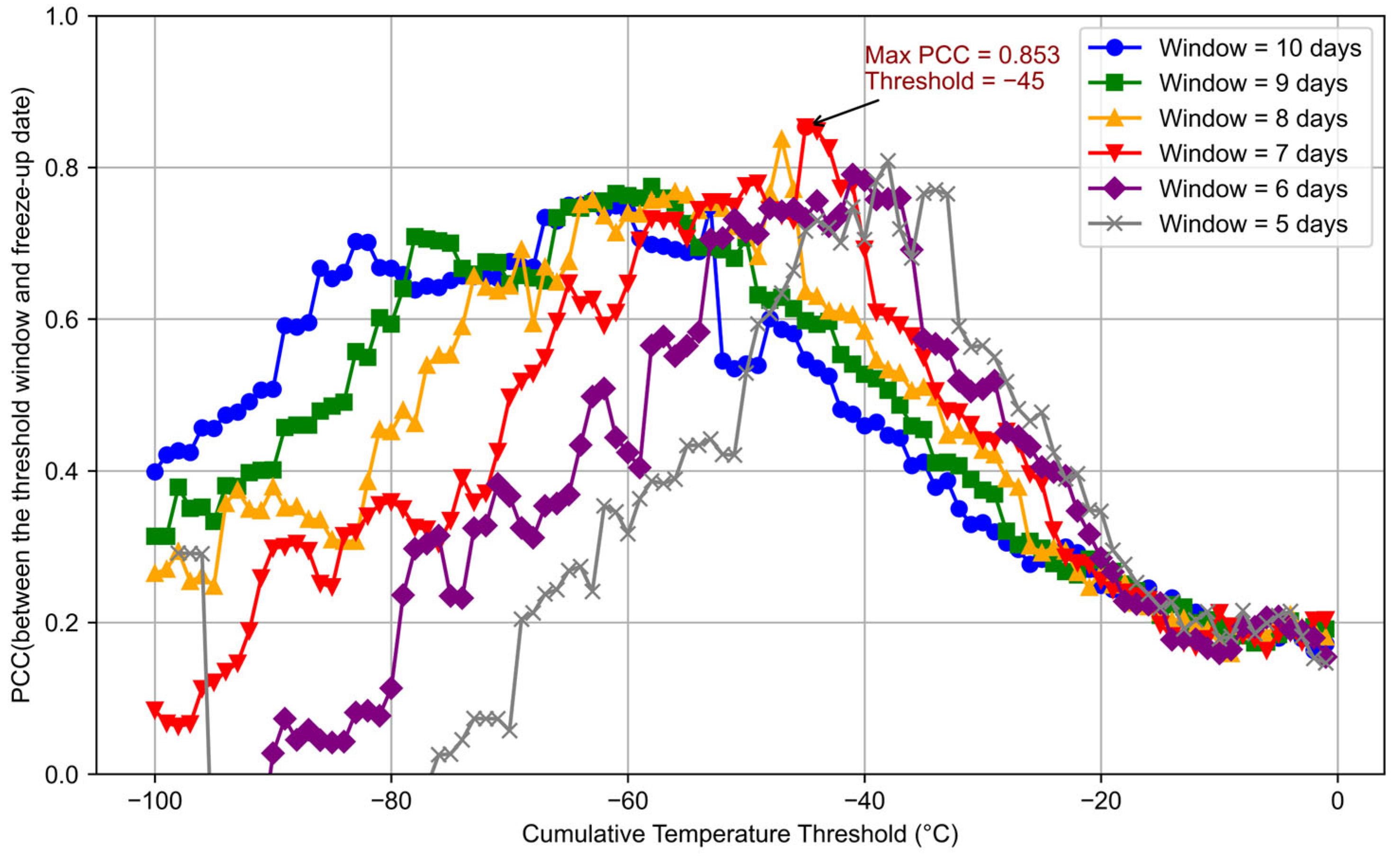
It should be noted that to determine the optimal sliding window (w) and threshold for X16, we have designed a search process as follows: starting from November 1, cumulative temperature durations are calculated using sliding windows of 5–10 days. For each window, the duration that reaches a given temperature threshold is determined, and the window with the threshold and duration exhibiting the highest correlation (PCC) with the freeze-up date is selected as the final result (Figure 2). The specific steps are as follows:
  • Starting from 1 November, calculate the cumulative temperature within a sliding window:
C t ( w ) = j = 0 w 1 T t
where C t ( w ) represents the cumulative temperature over w days ( w 5 , 10 ) starting from day t, and T is the daily average temperature.
2.
Given a threshold θ 100 , 0 , identify the first date that meets the threshold condition ( C t ( w ) < θ), and calculate the number of days from 1 November (Dy (w, θ)), y denotes the year.
3.
Traverse different thresholds and time windows, calculate the PCC value between Dy (w, θ) and the observed freeze-up date Fy for each combination, and finally determine the optimal threshold θ* time window w*, corresponding to the maximum PCC value, the PCC formula is given as follows:
P C C = y = 1 n ( D y ( w , T ) D ¯ ) ( F y F ¯ ) y = 1 n ( D y ( w , T ) D ¯ ) 2 i = 1 n ( F y F ¯ ) 2
where n denotes the number of years considered, D ¯ is the mean value across all years Dy (w, θ), and F ¯ is the mean freeze-up date.
The final result w* and θ* obtained is defined as the cumulative temperature factor X16.

2.3. Methods

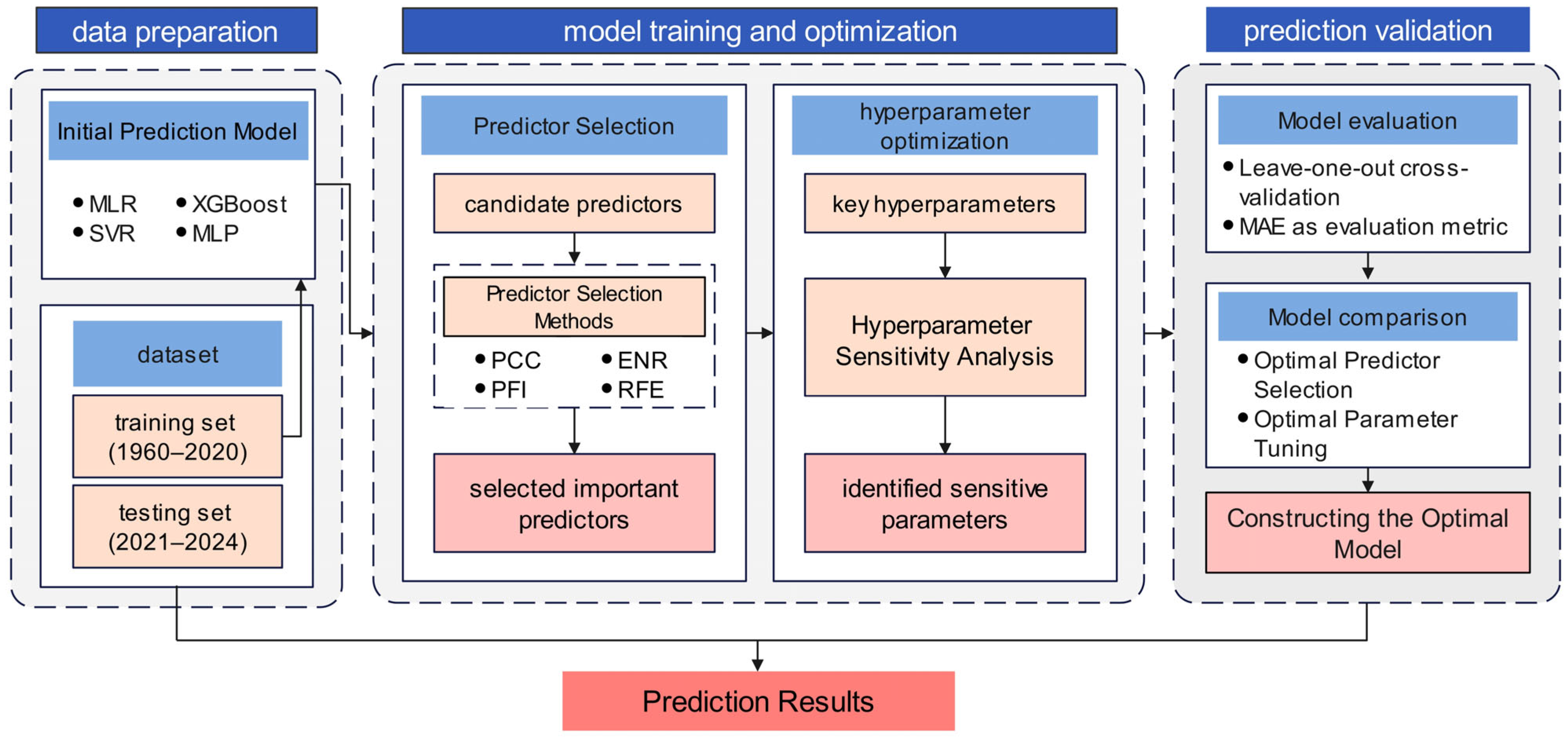
This study develops a systematic workflow for freeze-up date prediction, consisting of three stages: data preparation, model training and optimization, and prediction validation (Figure 3). The dataset is divided into a training set (1960–2020, 61 years) and a testing set (2021–2024, 4 years). In the training stage, all candidate features are separately processed by four feature selection methods (PCC, PFI, ENR, RFE), and the top n features from each are input into four models (MLR, SVR, XGBoost, MLP). Model performance under different feature sets and dimensions is systematically evaluated to determine the optimal configuration. Subsequently, parameter sensitivity analysis is performed, and hyperparameter tuning is applied to the sensitive parameters to improve model accuracy and stability. The entire evaluation uses leave-one-out cross-validation with MAE as the main metric. Finally, the optimal feature–parameter configurations are applied to the testing set, and predicted freeze-up dates are compared with observations to validate forecasting performance. All modeling and analyses were implemented in Python (version 3.10.18) using the scikit-learn and XGBoost machine learning libraries.

2.3.1. Predictor Selection Methods

In modeling freeze-up date prediction, the selection of input predictors critically influences both accuracy and generalization. To eliminate redundancy and improve model performance, four representative predictor selection methods are applied.
  • Pearson Correlation Coefficient (PCC)
PCC selects predictors based on the strength of their linear relationship with the target. It is calculated as the ratio of the covariance between the predictor and the target to their respective standard deviations (Equation (3)), with an absolute value close to 1 indicating higher correlation. PCC is computationally efficient, provides intuitive and interpretable results, but can only capture linear relationships [20].
2.
Permutation Feature Importance (PFI)
PFI evaluates the impact of perturbing input predictors on model performance to determine their relative importance. The model is trained using the original data, and the performance metric (e.g., MAE) is calculated. Then, the values of each predictor are randomly permuted, and the permuted data is fed back into the model to recalculate the performance metric. The difference between the original model performance and the permuted model performance represents the importance of that predictor. This process is typically repeated multiple times for each factor to ensure the stability and reliability of the importance assessment. PFI is simple to implement and quantifies each predictor’s contribution to model performance, but it has relatively high computational costs [34].
3.
Elastic Net Regularization (ENR)
ENR is a linear model that performs feature selection by fitting the model and determining the coefficients of the predictors. It introduces both L1 and L2 regularization to constrain the model’s coefficients, reducing the coefficients of less important predictors, effectively filtering out irrelevant features, and retaining the most important predictors for model performance. ENR can handle multicollinearity, but it has limited effectiveness in selecting predictors with nonlinear relationships, and its performance heavily depends on careful tuning of the regularization parameters [35].
4.
Recursive Feature Elimination (RFE)
RFE is a feature selection method that recursively removes the least important predictors. It starts by training the model with all available features and evaluates the importance of each feature. Then, it removes the least important features and retrains the model with the remaining ones. This process is repeated until the desired number of features is reached, helping RFE identify the most relevant predictors for the model. RFE can consider the interaction effects between features but may get stuck in local optima, leading to suboptimal feature selection results [36].

2.3.2. Prediction Models

To comprehensively evaluate the applicability and performance of different modeling approaches for freeze-up date prediction, four representative models from both statistical and machine learning categories are employed:
  • Multiple Linear Regression (MLR)
MLR [9] is a commonly used linear prediction model that predicts outcomes by fitting the linear relationship between predictor variables and the target variable. It establishes a regression equation to describe the relationship between them and uses the least squares method to determine the regression coefficients, minimizing the sum of squared errors between predicted and actual values. The unexplained random error is treated as the intercept. MLR offers stable performance, strong interpretability, and low computational cost, making it the most widely used model in Yellow River ice forecasting [14]. Its reliability has been repeatedly validated through long-term applications, but its expressive capability is limited under complex conditions.
2.
Support Vector Regression (SVR)
SVR is a regression prediction method based on support vector machines, which, unlike traditional regression methods, can tolerate a certain level of prediction error. Its goal is to keep most of the sample data within a specified error threshold, with the size of the error controlled by the penalty factor C. For data points that exceed the threshold, SVR imposes a penalty, thus preventing overfitting while maintaining prediction accuracy. As a result, SVR is capable of handling nonlinear problems and exhibits strong robustness, often performing exceptionally well in the presence of significant data noise. SVR has been successfully applied to ice prediction in the Yellow River, achieving good prediction accuracy; however, its performance is significantly influenced by the choice of kernel function and its parameters [21].
3.
Extreme Gradient Boosting (XGBoost)
XGBoost is an efficient decision tree algorithm based on the gradient boosting framework. As an ensemble learning method, the core idea of gradient boosting machines is to build a strong learner by combining multiple decision trees. Each decision tree divides the data into different groups by optimizing the predictive thresholds of features to generate output estimates. The goal of the gradient boosting algorithm is to iteratively reduce errors, meaning that each new model focuses on correcting the residuals (i.e., prediction errors) of the previous model, continuously adjusting to improve the overall model’s predictive accuracy. XGBoost effectively captures nonlinear relationships and interactions between variables, and it enhances its resistance to overfitting through mechanisms like regularization. However, as an ensemble model, XGBoost has a relatively complex structure and limited interpretability [37]. Although its application in Yellow River ice forecasting remains limited, studies on the Heilongjiang [20] and Warta Rivers [38] have demonstrated its high predictive accuracy.
4.
Multilayer Perceptron (MLP)
MLP is a feed-forward artificial neural network comprising an input layer, one or more hidden layers, and an output layer. The input layer receives external data and transfers it into the network, where it is initially processed and stored in vectors for easy access by the hidden layers. The hidden layers perform feature mapping, transforming lower-order features into higher-order ones, allowing the network to uncover meaningful internal representations from relatively small datasets and improving learning performance. The output layer then maps these internal representations back to the original space to generate forecasts based on the input signals [24]. MLP is capable of learning complex nonlinear relationships through multiple hidden layers, giving it strong expressive power. However, this also makes the training process complex, and the model is prone to being influenced by noise and small sample sizes, leading to unstable results and a higher risk of overfitting. It has been successfully applied to Yellow River ice forecasting and achieved promising predictive accuracy [29], but its stability can be insufficient [39].

2.3.3. Hyperparameter Sensitivity Analysis and Optimization

To enhance both the predictive performance and generalization capability of the models, a systematic hyperparameter sensitivity analysis and automated tuning procedure were implemented during model development. Specifically, for the base predictive models (SVR, XGBoost, and MLP), a univariate sensitivity analysis was first conducted by perturbing each key hyperparameter individually and recording the resulting changes in model error. The impact of each hyperparameter on predictive performance was quantified using ΔMAE, defined as the difference in mean absolute error (MAE) before and after perturbation.
Based on the sensitivity ranking of hyperparameters for each model, highly sensitive parameters were further optimized using a Bayesian optimization-based framework (Optuna) [40]. Unlike traditional grid search or random search methods, this approach efficiently identifies the optimal parameter combination with a lower evaluation cost. During the tuning process, each candidate parameter set was evaluated through cross-validation on the training set, using MAE as the objective function, thereby ensuring a balanced trade-off between model stability and predictive accuracy.

2.3.4. Leave-One-Out Cross-Validation

Given the limited historical records of freeze-up dates in the NIM reach of the Yellow River (1960–2024, 65 samples), leave-one-out cross-validation (LOOCV) was employed to maximize data utilization and obtain robust model evaluation results. LOOCV is an extreme form of k-fold cross-validation (with k = n), in which, during each iteration, a single sample is held out as the validation set while the remaining n-1 samples are used for training. This process is repeated n times, ensuring that each sample serves exactly once as the validation set [41]. The overall model performance is then assessed by averaging the performance metrics across all iterations. Compared with conventional k-fold methods (e.g., 5-fold or 10-fold), LOOCV fully leverages all available samples for both training and validation, thereby significantly reducing evaluation bias under small-sample conditions and avoiding the loss of training data due to validation set partitioning [42].

2.3.5. Evaluation Metric

To assess the performance of each predictive model for freeze-up dates, the mean absolute error (MAE) was adopted as the sole evaluation metric. Compared with other error measures, MAE directly quantifies the average deviation, in days, between predicted and observed freeze-up dates, aligning closely with the practical requirements for forecasting accuracy. MAE is calculated as follows:
M A E = 1 n i = 1 n y i y ^ i
where yi is the observed freeze-up date in year i, y ^ i is the model-predicted freeze-up date for year i, and n is the total number of samples.
Under the LOOCV framework, each year in the training set is sequentially used as the validation sample while the remaining years serve as the training set, resulting in m rounds of training and prediction. In each iteration, the model’s prediction for the left-out sample is recorded. The MAE is then computed by aggregating the errors across all iterations:
M A E L O O C V = 1 m i = 1 m y i y ^ ( i )
where y ^ ( i ) denotes the prediction for the sample obtained from the model trained on all other samples.

3. Results

3.1. Predictor Selection Results and Evaluation

In the feature selection process, different methods focus on different evaluation criteria, such as feature correlation, contribution to model performance, and feature importance scores [20]. As a result, different methods may yield different feature sets. Since each model has distinct algorithmic characteristics and adaptability, the choice of input factors can significantly impact prediction performance [26]. Therefore, we evaluate the feature sets selected by different methods and input them into each model to determine the most suitable set of input factors for each model.
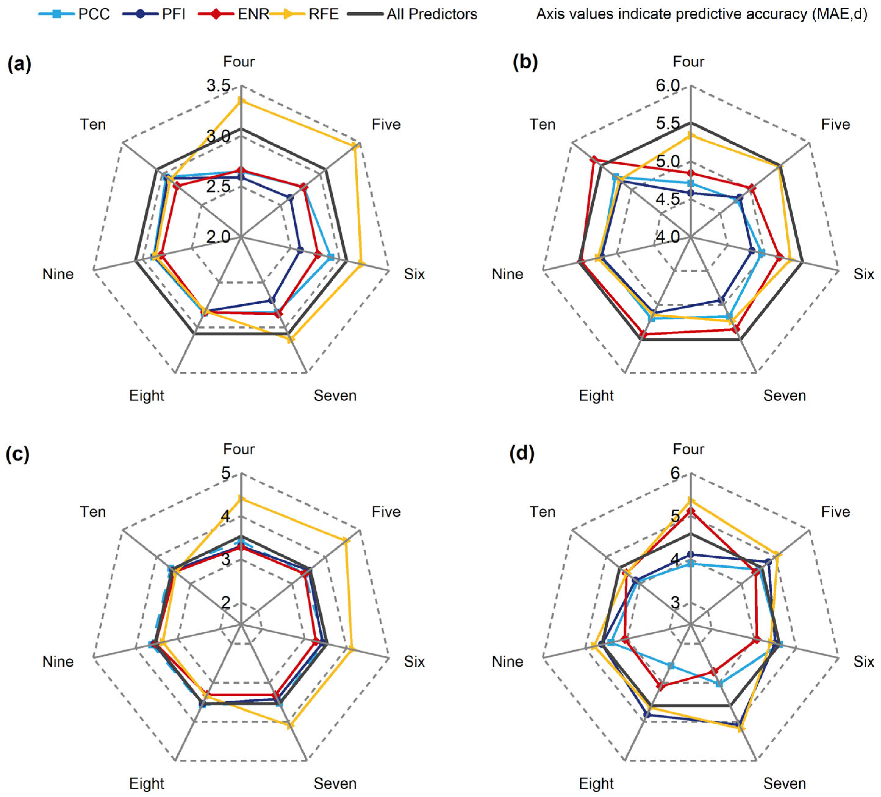
This study employed four feature selection methods (PCC, PFI, ENR, and RFE) to evaluate the predictive performance of different sets of input predictors, including varying numbers of predictors and the full set of 16 candidate predictors, under a leave-one-out cross-validation framework. Based on these evaluations, the optimal feature selection method and the corresponding input predictor combination (Table 2) were determined for each of the four predictive models (MLR, SVR, XGBoost, and MLP). The results indicate that all four models achieved a 7.6–23% improvement in predictive accuracy when using the selected predictors compared with using all predictors (Table 2), highlighting the importance of predictor selection in freeze-up date forecasting. Moreover, the optimal feature selection method and the number of predictors varied notably among models (Figure 4). For MLR, using 4–6 core predictors selected by PFI consistently yielded the best or near-best predictions. SVR performed best with a 4-predictor scheme also selected by PFI. XGBoost exhibited low sensitivity to the selection method or predictor count under PCC, PFI, or ENR, showing minimal fluctuation in accuracy. In contrast, MLP was more sensitive to the choice of input predictors and achieved optimal performance when the top 8 predictors selected by PCC were used.
Based on the performance of different feature selection methods, PCC, PFI, and ENR demonstrate higher alignment with the freeze-up date prediction target and are the primary contributors to improved model performance. These three methods show a largely consistent predictor ranking strategy (Table 3), placing X16 (Number of days until the 7-day cumulative air temperature drops below −45 °C) at the top, while frequently selecting predefined-window cumulative temperature predictors (X11, X12, X13) and reach-averaged flow predictors (X4, X5). Since both thermal and hydrodynamic factors are critical drivers of river ice formation [4,43], incorporating them together enables the models to better capture the underlying processes and achieve strong predictive performance. In contrast, although RFE also identifies X16 as the most important predictor, its selection of leading predictors differs noticeably from the other three methods. By incorporating some marginal extreme-temperature predictors (e.g., X14, X15), the relative importance of hydrodynamic predictors is reduced, leading to slightly lower overall prediction performance compared to PCC, PFI, and ENR. This discrepancy likely stems from RFE getting trapped in a local optimum during feature selection, affecting its ability to retain more useful predictors. Therefore, it is crucial to carefully select both the predictive factors and the appropriate selection method for each model.

3.2. Hyperparameter Sensitivity Analysis and Calibration Results

Bayesian optimization was used to adjust the hyperparameters of SVR, XGBoost, and MLP models. This method efficiently handles the complex interactions between hyperparameters, helping to find the optimal solution. To enhance computational efficiency, a sensitivity analysis was first conducted (Table S1), focusing on tuning the most impactful parameters. Each model was optimized for 50 iterations, taking approximately 3–5 min.
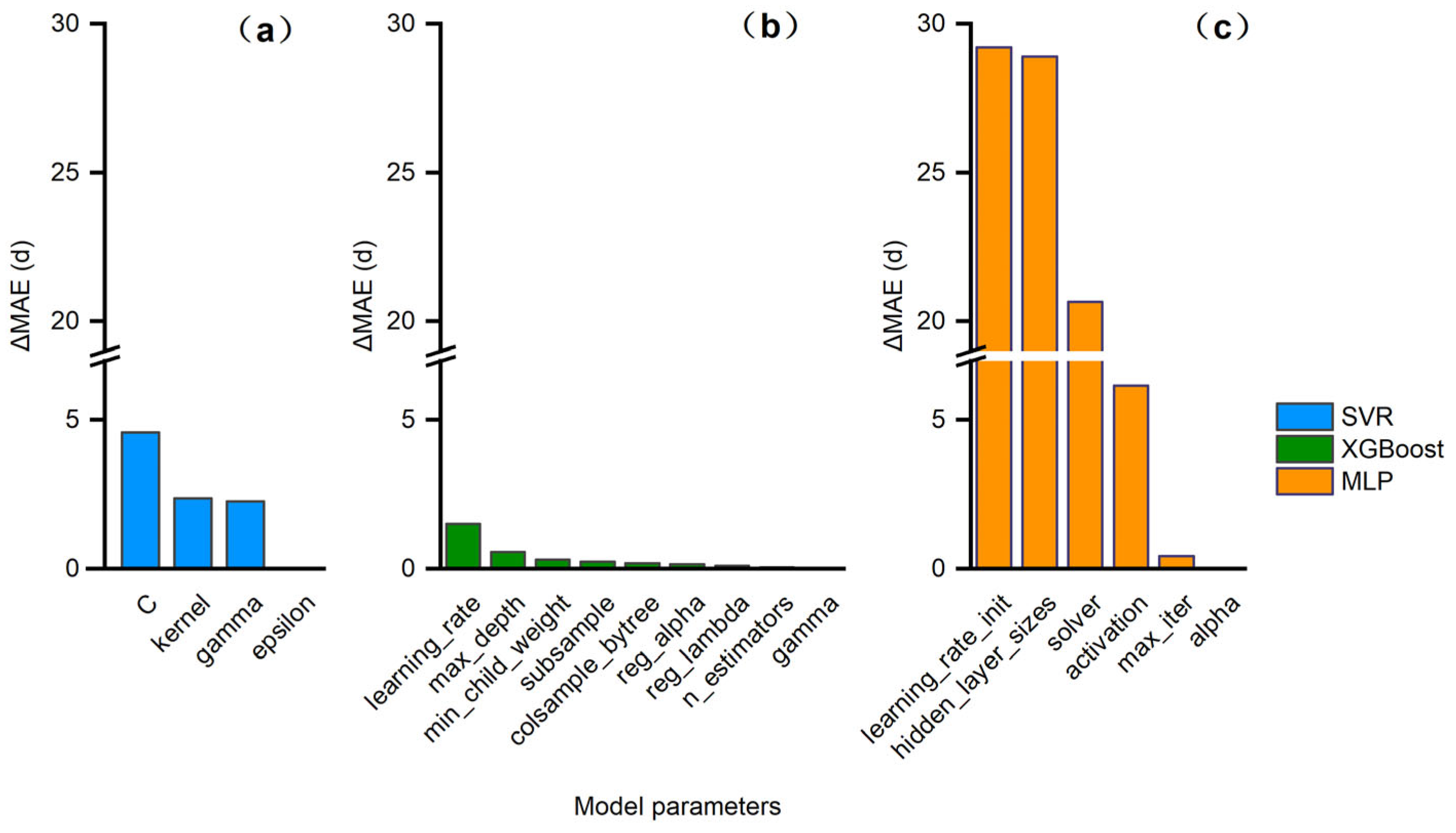
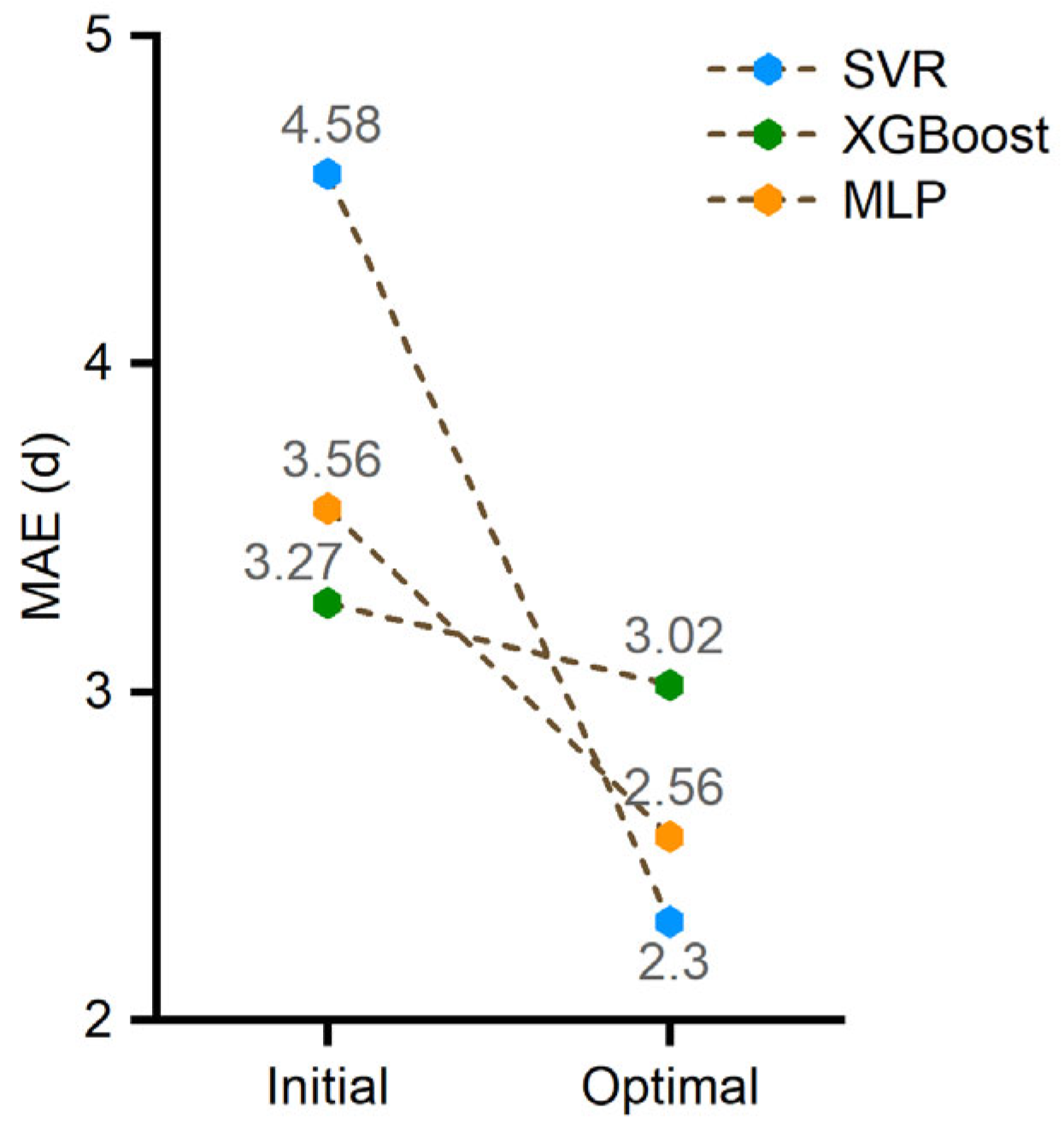
The hyperparameter sensitivity analysis of each model (Figure 5) allowed the identification and subsequent tuning of key hyperparameters for SVR, XGBoost, and MLP (Table 4). After calibration, all three models showed significant improvements in predictive performance, with errors reduced by 0.25–2.28 d (Figure 6), demonstrating the effectiveness of the optimization strategy in enhancing model accuracy.
Analysis of the parameter sensitivity results (Table S2) revealed that different models exhibit distinct responses to hyperparameters. MLP was found to be the most sensitive, with certain parameters, particularly learning_rate_init, causing a substantial change in predictive performance (ΔMAE = 29.2147 d). SVR was relatively stable but still showed notable sensitivity to C (ΔMAE = 4.5889 d). In contrast, although XGBoost has many hyperparameters, it was the least sensitive among the three models, with the most influential parameter, learning_rate, yielding only ΔMAE = 1.5122 d. By precisely optimizing these sensitive parameters, the MAELOOCV of SVR and MLP decreased substantially compared to the default settings, by 46% and 27%, respectively. XGBoost also benefited from parameter tuning, achieving a 4.5% reduction in MAELOOCV, demonstrating both its robustness and potential for further improvement.

3.3. Evaluation of Different Modeling Strategies Under Anthropogenic Influences

3.3.1. Impact of Human Intervention

Human intervention, particularly reservoir operations, has significantly altered the hydrological evolution of the NIMRYR. As the Liujiaxia, Longyangxia, and Haibowan reservoirs were successively put into operation, their effects on the river became increasingly evident, involving flow, river morphology, and water temperature.
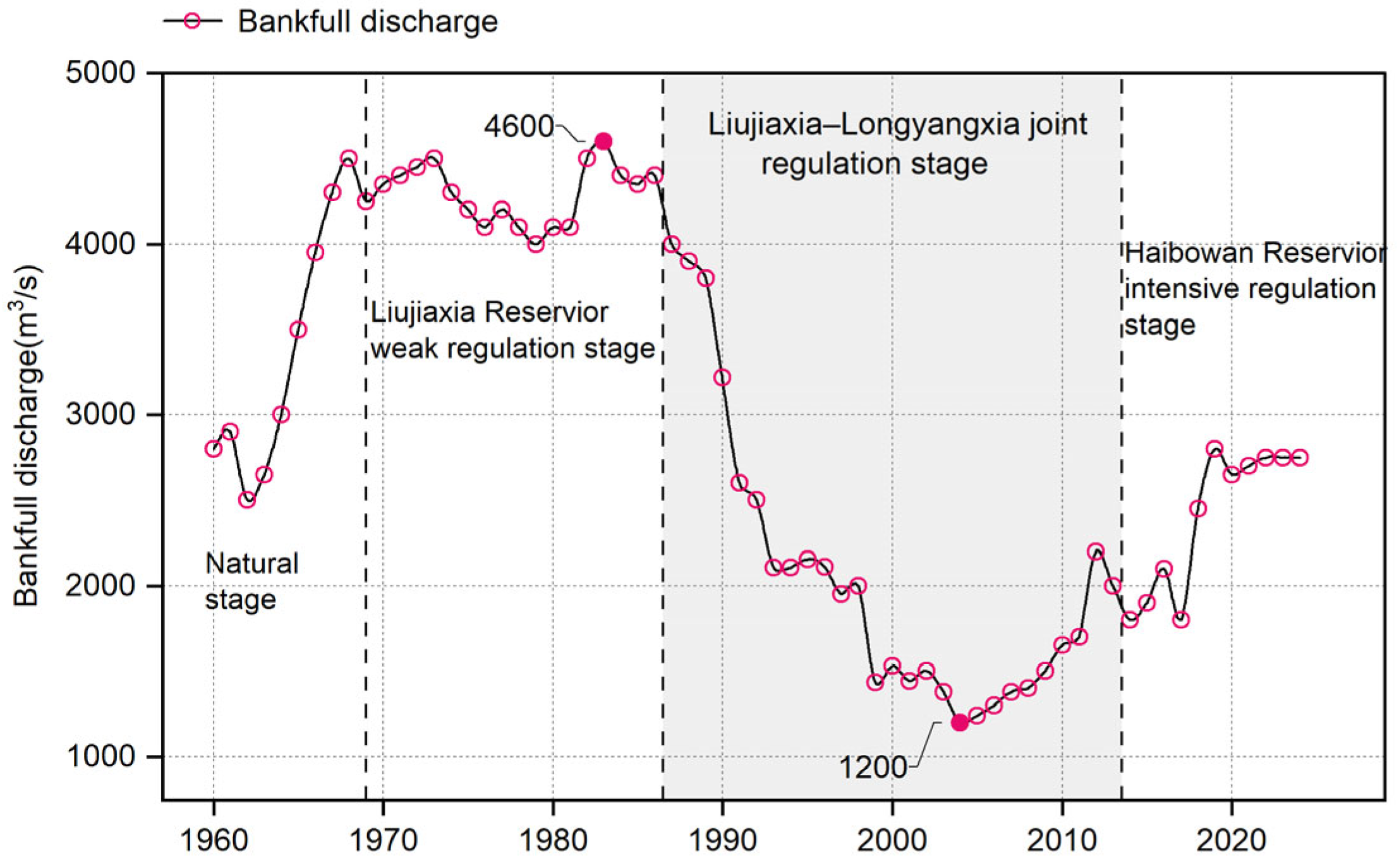
Compared to the natural state, the operation of these reservoirs, including Liujiaxia, altered the seasonal distribution of runoff, increasing the proportion of flow during the ice period (November to March of the following year) in the hydrological year (July to June of the following year) from 24% to 38% (Figure S2), resulting in an increase in ice period runoff in the NIMRYR from 6.109 billion cubic meters to 6.989 billion cubic meters (Table S3). Changes in seasonal flow distribution reduced peak flows into the Inner Mongolia reach, lowered flood season water volume, diminished sediment transport, aggravated sedimentation, and decreased the bankfull discharge (Figure 7) [12]. During the period of Liujiaxia’s solo operation, its relatively weak regulation capacity (with a storage volume of 5.7 billion m3) led to a slow decrease in bankfull discharge. Although a series of wet years between 1981 and 1986 temporarily restored flow through floodwater flushing, the combined operation of Liujiaxia and Longyangxia reservoirs after 1987 significantly exacerbated this decline, and with reduced runoff, the flow capacity rapidly decreased, causing increased river sedimentation. It was only after the 2018–2020 flood seasons, which had sustained high-flow periods, that the bankfull discharge gradually began to recover. However, it still did not return to levels seen before 1987. Reservoir construction and operation also significantly influenced water temperature. River freezing in the Yellow River typically occurs between the Sanhuhekou and Toudaoguai Reaches, at over 1200 km from Liujiaxia and Longyangxia reservoirs, so these reservoirs had little impact on water temperature during freezing. However, Haibowan Reservoir’s operation significantly increased downstream water temperature [31]. Before the operation of Haibowan Reservoir, the average air temperature at the Bayangaole station in early November was 3.88 °C, and the average water temperature was 7.30 °C. After the reservoir’s operation, the air temperature rose to 4.51 °C, and the water temperature increased to 8.74 °C (Table S4). Based on this, we infer that the reservoir caused an approximate 1 °C increase in water temperature under similar atmospheric conditions.
As the reservoirs have gradually come into operation, human intervention in the NIMRYR has steadily intensified, causing the river’s hydrological characteristics to increasingly deviate from their natural state. This change has significantly impacted ice conditions and heightened the uncertainty of freeze-up date prediction. Therefore, human interference should be considered when constructing prediction models.

3.3.2. Selection of Different Sample Periods Based on Major Reservoir Construction

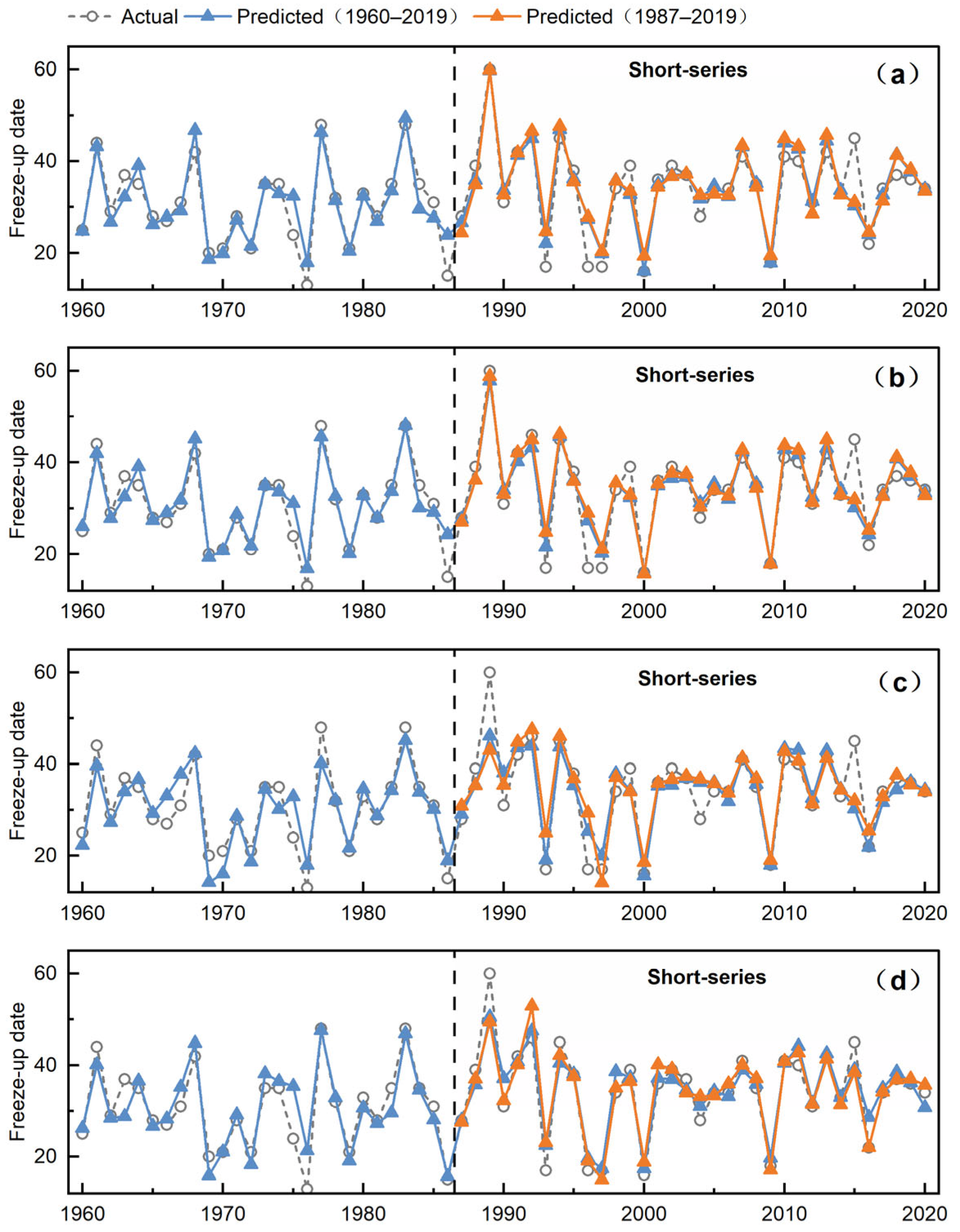
Based on freeze-up observations from the NIMRYR, two sets of training datasets were constructed: a long-term series covering 1960–2020 with complete records, and a shorter series spanning 1987–2020 following the completion of the Longyangxia Reservoir. The impact of different sample periods on model accuracy was compared. Four predictive models (MLR, SVR, XGBoost, and MLP) were trained and evaluated using LOOCV. The mean absolute error over the 1987–2020 period (MAELOOCV) from both datasets was used as the accuracy metric to systematically assess the adaptability and stability of the models under different data backgrounds. The results shown in Figure 8 indicate that using the short-sequence dataset does not effectively improve model accuracy, and different models respond differently to the choice of data length. For MLR, SVR, and XGBoost, MAELOOCV is lower on the long-sequence dataset (2.45 d, 2.30 d, and 3.02 d) than on the short-sequence dataset (3.04 d, 2.52 d, and 3.22 d), while MLP performs slightly better on the short-sequence data, with MAE decreasing from 2.56 d to 2.27 d. Therefore, in model construction, we cannot, as previous studies have done, simply discard early observations to account for the effects of human interventions.

3.3.3. Incorporating Stage-Specific Threshold Cumulative Temperature Predictor

The previous analysis indicated that altering the sample period did not effectively improve model accuracy. Therefore, we begin with predictor X16 (Number of days until the 7-day cumulative air temperature drops below −45 °C), the core variable consistently identified by all four feature selection methods, and incorporate the context of different reservoir construction periods into this factor. The temperature threshold of −45 °C for this predictor was originally determined through optimization based on the full training dataset (1960–2020). However, this unified threshold overlooks the variations in the temperature–freeze-up response under different hydrological regulation regimes. To address this, the study divides the period of 1960–2024 into four stages [12,31]: the natural stage (1960–1968), the Liujiaxia Reservoir weak regulation stage (1969–1986), the Liujiaxia–Longyangxia joint regulation stage (1987–2013), and the Haibowan Reservoir intensive regulation stage (2014–2024). Using the method introduced in Section 2.2, the optimal temperature thresholds and time windows for each stage were determined (Table 5). These were then integrated to construct a stage-specific cumulative temperature predictor, which, together with other influencing factors, was used for model training. This allowed the model to account for different reservoir regulation backgrounds and better capture the response relationship between temperature and the freeze-up process.
Table 5 shows that human interventions have notably altered the cumulative thermal conditions required for freeze-up. During the Liujiaxia Reservoir weak regulation stage, the average daily cold intensity is similar to the natural stage, but a higher-intensity accumulation within a shorter period is needed. This is due to the increased ice-period runoff, which requires more intense cooling for freeze-up. In the Liujiaxia–Longyangxia joint regulation stage, both total and daily cold requirements decrease. During this period, the bankfull discharge capacity drops by approximately 52% (Figure 7), significantly increasing the likelihood of freeze-up and allowing it to occur at higher temperatures. In the Haibowan Reservoir intensive regulation stage, a larger amount of cumulative cold is required to trigger freeze-up. This change is mainly due to the rise in river water temperature, along with increased runoff and a 17% recovery in bankfull discharge, all of which raise the thermal threshold for freeze-up. These stage-specific cumulative temperature thresholds were considered consistent with the observed hydrological and thermal conditions and were therefore integrated to construct a Stage-Specific Cumulative Temperature Predictor. This predictor, together with other influencing factors, was used for model training, enabling the model to account for different reservoir regulation stages and better capture the temperature–freeze-up response.
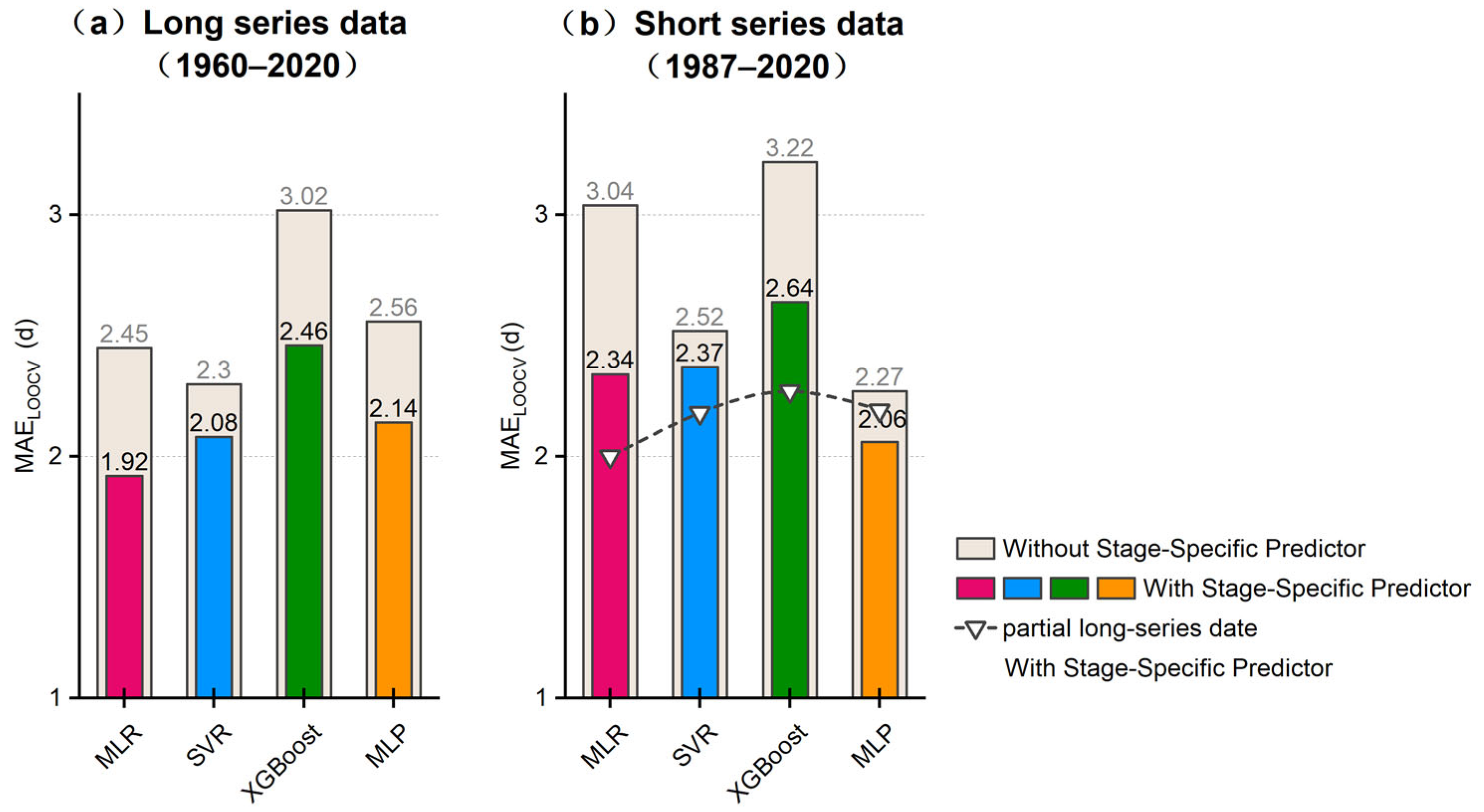
The results indicate that incorporating the Stage-Specific Predictor, which reflects different reservoir regulation stages, significantly improves overall model accuracy, reducing the MAE by 0.15–0.7 d (Figure 9). Using the long-sequence data from 1960 to 2020, the MAELOOCV of all models decreased noticeably. Among them, MLR and XGBoost showed the most substantial improvements, with MAELOOCV reductions of approximately 20%, while SVR and MLP achieved error reductions of 10% and 16%, respectively. Further analysis using the short-sequence data from 1987 to 2024 also showed clear improvements for all models, with reductions of 23%, 6%, 18%, and 9%, respectively. Notably, when comparing the long- and short-sequence results under identical modeling conditions with the Stage-Specific Predictor incorporated, the long-sequence data still held a slight advantage: MLR, SVR, and XGBoost exhibited MAELOOCV lower by 0.42 d, 0.29 d, and 0.18 d, respectively, whereas MLP was slightly higher by 0.08 d. Further comparison revealed that MLR achieved the highest accuracy on the long-sequence data (1.92 d), primarily because the extended dataset encompassed a wider range of climatic backgrounds and human interventions. The introduction of the Stage-Specific Predictor helps the model extract common features across different periods, stabilizing the training process [44]. In contrast, MLP performed best on the short-sequence data (2.06 d) due to its stronger nonlinear fitting capability, making it more suitable for capturing ice dynamics under the complex disturbances of recent decades [29,45]. However, this also suggests that the long-sequence data may have contained potential biases that could have interfered with the model, such as inaccuracies in measurement instruments, the reliability of manual observations, and inconsistencies in recording standards. Overall, incorporating the Stage-Specific Predictor, which defines period-specific temperature thresholds, substantially improves model forecasting performance compared to merely adjusting sequence length. This approach also mitigates the effects of human interventions, particularly reservoir joint operations.

3.4. Prediction Results

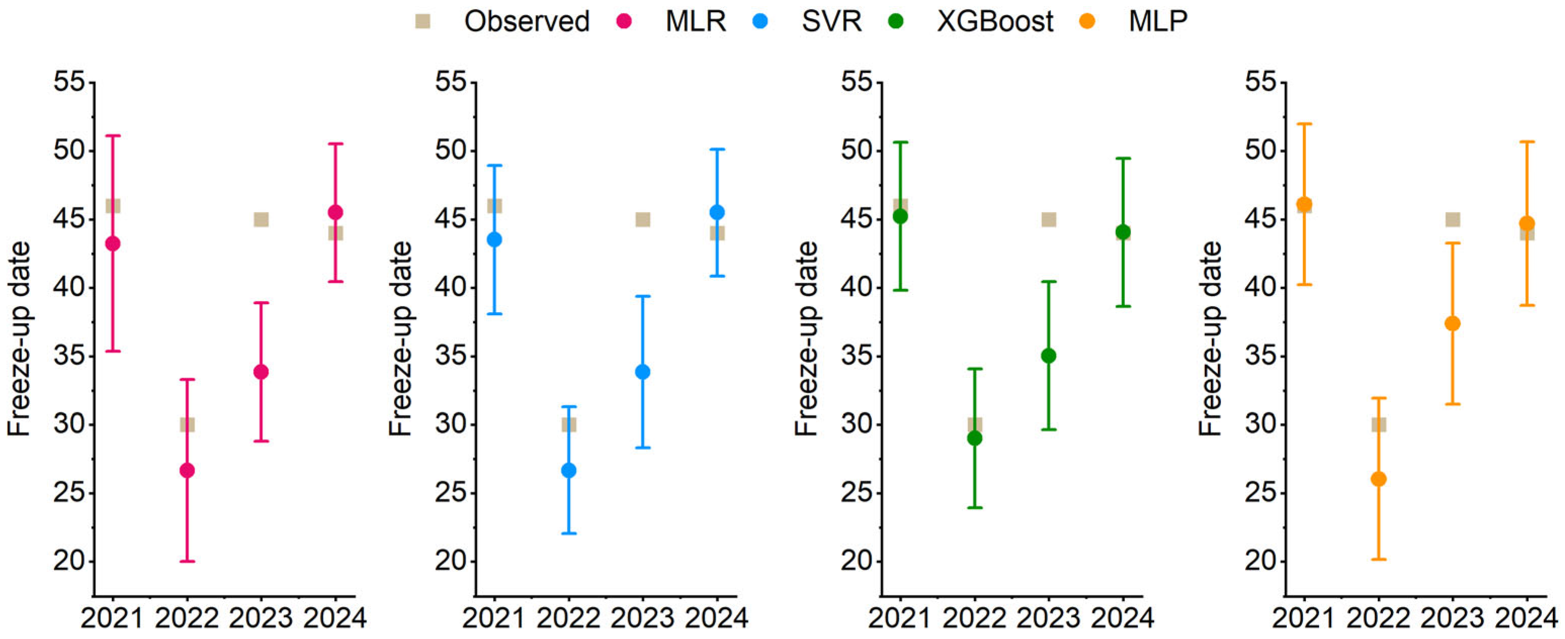
Based on the model construction and accuracy verification using LOOCV described above, this section further evaluates the models’ predictive performance in real-world scenarios (Figure S3). To this end, data from 2021 to 2024 were selected as the test set. Using the previously determined optimal factor combinations, model parameters, and Stage-Specific Predictor strategy, models were constructed and annual predictions were performed. Based on the prediction results shown in Table 6, the models achieved optimal errors of 0.16 d, −0.99 d, −7.61 d, and 0.07 d for 2021–2024, respectively, indicating that they retain strong generalization capability for practical forecasting. Comparing the models, those capable of nonlinear modeling exhibit stronger adaptability than linear models in freeze-up date prediction tasks, which is consistent with previous studies on ice process forecasting [9,21,29,44]. Specifically, XGBoost achieves consistently low prediction errors in 2021, 2022, and 2024 (MAE = 0.77 d, 0.99 d, and 0.07 d, respectively). However, 2023 represents a year with generally higher prediction difficulty for all models. In this challenging year, MLP outperforms the others, exhibiting errors 2.03–3.54 d smaller than XGBoost, SVR, and MLR, suggesting that it may better handle complex freeze-up conditions [5].

3.5. Uncertainty Analysis

To assess the prediction uncertainty of the models, this study used a Monte Carlo simulation approach [24], generating 500 error scenarios based on the prediction errors from the training dataset. The prediction confidence intervals for the MLR, SVR, XGBoost, and MLP models were then calculated and visualized (Figure 10). In terms of interval characteristics, Support Vector Regression (SVR) demonstrated the best prediction stability, with the narrowest average 90% confidence interval width (9.34 days), which aligns with its good adaptability to small sample data scenarios. In contrast, although XGBoost performed well in terms of overall prediction accuracy, its 90% confidence interval had the widest average bandwidth (13.03 days), indicating higher uncertainty.
In 2023, the actual freeze-up date did not fall within the confidence interval of any model, and all models exhibited significant prediction errors, with the maximum error reaching 11.15 days (MLR). Compared to the freeze-up dates in 1962, 1985, and 1990, which occurred under similar temperature and flow conditions, the freeze-up in 2023 was notably delayed (Figure 11). We hypothesize that the deviation in 2023 is not a typical error, but rather the result of a combination of climate anomalies and human interventions. Regarding climatic conditions, in 2023, the temperature distribution in the NIMRYR exhibited a west-high, east-low pattern, with considerable temperature fluctuations. In November, the temperature at the Bayangaole station was 0.3 °C higher than the 1960–2024 average, while temperatures at Baotou and Todaoguai stations were 1.0 °C and 1.1 °C lower, respectively. In early December, all three stations experienced significant warming, with temperatures 5.9 °C, 3.1 °C, and 3.9 °C higher than the average, approaching the highest values for the period (Table S5). In terms of hydrological conditions, human regulation had a significant impact on flow. In November, the average flow in the reach was only 577 m3/s, but by the end of the month, the flow suddenly increased, with the average flow from November 27th to freeze-up reaching 723 m3/s (Figure S4). Due to the near absence of effective precipitation in the Inner Mongolia winter reach, this fluctuation in flow was primarily driven by human activities such as reservoir regulation and water diversion projects. It is worth noting that the MLP model, by incorporating the short-term flow fluctuation factor (x1), effectively captured the flow changes induced by human regulation, thereby reducing the prediction bias caused by human interference. Thus, models relying solely on stage-specific predictors may struggle to fully account for complex freezing scenarios. The evolution of river ice is influenced by a combination of human interventions, climate change, and other factors, with existing models lacking the responsiveness to these atypical scenarios, which constitutes a major source of model uncertainty. The complexity and dynamic nature of these factors extend beyond the predictive range of current models, and future research needs to enhance the identification and modeling of these disturbance factors.

4. Discussion

4.1. Differences in Prediction Accuracy Among Models

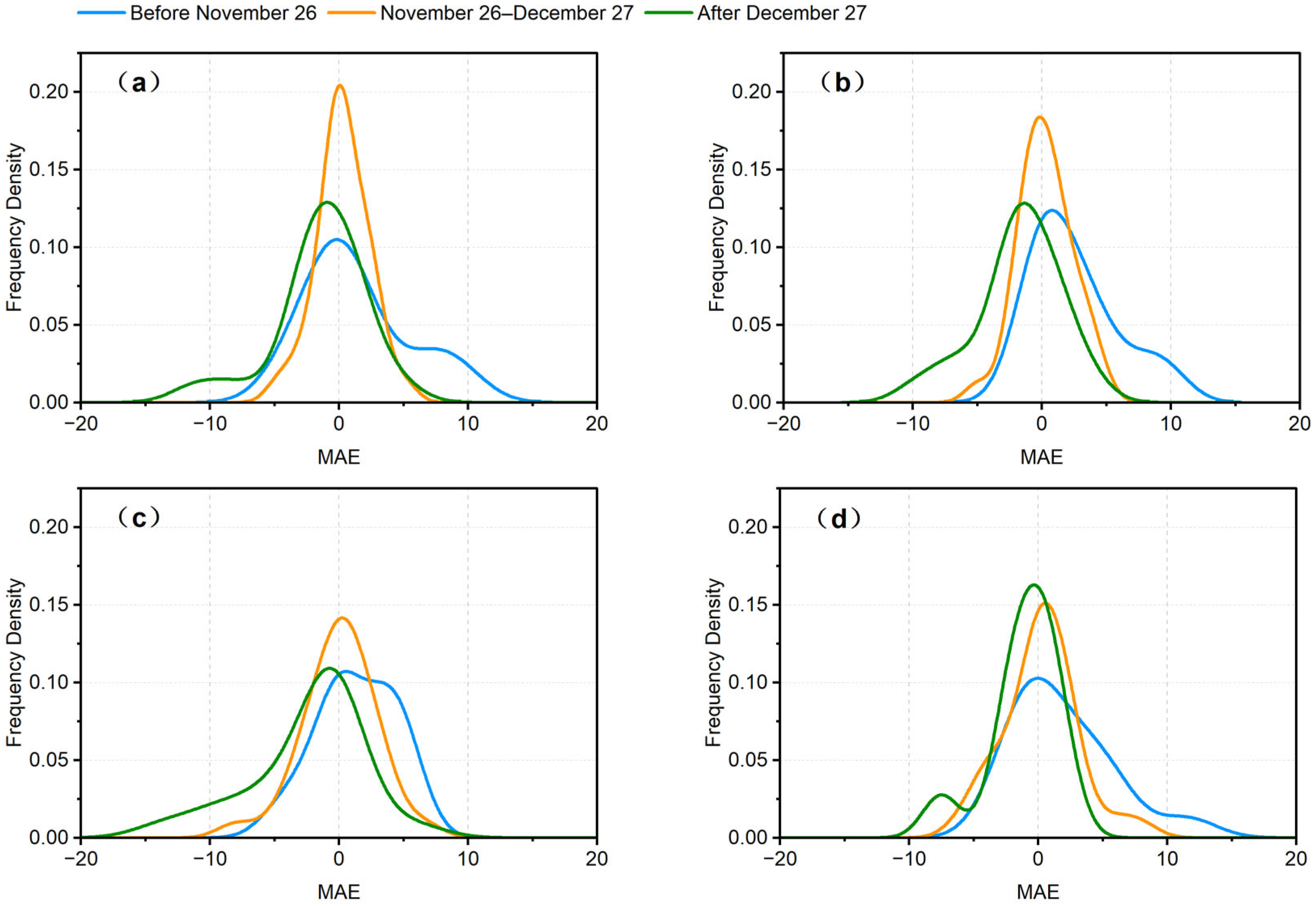
The four prediction models exhibit distinct differences in forecasting accuracy for freeze-up dates. Based on the results (Section 3.4), XGBoost achieved the highest accuracy with an MAE of 2.95 d, followed by MLP at 3.11 days. Both models demonstrate a favorable balance of flexibility and stability across most scenarios, whereas SVR and MLR show relatively larger deviations, with MAEs of 3.91 d and 4.69 d, respectively. A detailed analysis of the frequency density distribution of prediction errors for 65 freeze-up dates from 1960 to 2024 reveals (Figure 12) substantial variation in model performance across different dates. Predictions are generally more accurate around 2 December. For early freeze-up dates prior to 26 November, XGBoost exhibits relatively small errors, with a concentrated error distribution and short tails, indicating a low probability of large deviations and high stability. During the concentrated freeze-up period between 26 November and 7 December, MLR achieves the best accuracy and stability, with errors tightly clustered and deviations minimized, followed by SVR. For late freeze-ups, occurring from 8 December to the latest recorded date, MLP performs best, effectively capturing the characteristics of delayed freeze-up events with relatively small errors, whereas XGBoost’s accuracy declines and may exhibit extreme deviations in certain years.
Annual analyses further confirm these patterns. For the years with relatively early freeze-ups, 1975 and 2016, MLP exhibited large deviations (MAE = 11.56 d and 4.86 d), as rapid temperature drops driven by strong cold waves led to only 1–2 days between the initial appearance of drift-ice and the onset of freeze-up. In contrast, in 1986, also an early freeze-up year, MLP performed exceptionally well, with a deviation of just 0.01 days. This was because, unlike 1975 and 2016, the early freeze-up in 1986 was caused primarily by limited channel discharge and ice jams forming at bends, rather than rapid temperature changes. These results indicate that MLP’s nonlinear learning capability is advantageous under conditions dominated by non-meteorological factors but less adaptive when abrupt temperature–freeze relationships occur. XGBoost, on the other hand, performed best in 1975 and 2016 (MAE = 5.41 d and 0.03 d) but exhibited significant deviation in 1989, the latest freeze-up year, with an MAE of 13.52 d. MLR predicted 1989 accurately (2.26 d), suggesting that even in this extreme year, the linear temperature–freeze relationship still held, whereas XGBoost’s extrapolation ability for extreme out-of-sample events was limited [46].
The differences in the predictors used by different models may be an important reason for the prediction discrepancies. MLR and SVR often show similar performance, likely due to their use of the same factors (Table 2), including cumulative temperature and average river flow during the freeze-up period, with SVR also employing a linear kernel function (Table 4). XGBoost introduces the key predictor X7 (Date of drift-ice appearance), which reflects the combined effects of factors such as flow and temperature on the water body, helping capture early signs of freeze-up and thus improving model accuracy in years with earlier freeze-up. The MLP model uses the most predictors (Table 2), learning richer information (e.g., X3) and, combined with its powerful learning capabilities, is better suited to handle complex and extreme freeze-up patterns. However, while more factors provide richer information, they may also introduce noise. In terms of the relationship between predictor selection and model performance, MLR, as a typical linear model, and SVR with a linear kernel tend to retain predictors with higher correlations or those that significantly improve performance, thus ensuring overall fit accuracy. In contrast, XGBoost and MLP, due to their inherent nonlinear learning capabilities, are able to extract patterns from a broader range of information, making them more adaptable to diverse scenarios.
A further tally of the optimal model type for each year under four construction strategies (long and short series, with or without Stage-Specific Predictors) indicates that (Tables S6–S9), among the 65 samples from 1960 to 2024, MLR, SVR, XGBoost, and MLP were the optimal choice 18, 11, 18, and 18 times, respectively (Table S10). These findings suggest that no single model can comprehensively achieve accurate freeze-up date forecasts. A more reasonable approach is to select models flexibly according to specific scenarios or to employ an ensemble modeling strategy that integrates multiple models [47], thereby enhancing the robustness and generalization capability of freeze-up date predictions.

4.2. Model Performance Under the Influence of Human Interventions

Human interventions significantly increased the prediction errors of freeze-up dates (Figure 13). During the weakly regulated period, prediction errors remained relatively low (1.80–2.08 d); following the commissioning of the Longyangxia Reservoir in 1987, errors still remained stable overall (2.07–2.20 d). However, in the period of intensive regulation from 2014 to 2024, prediction errors generally increased for most models (2.05–2.85 d), reflecting that complex operations, such as multi-reservoir joint regulation, have substantially disrupted the traditional relationships among air temperature, discharge, and freeze-up response. We further conducted a year-by-year analysis of prediction errors. In 2016 and 2020, during the intensive regulation period, sudden cold waves shortened the interval between the first appearance of drift-ice and freeze-up to only one day. In these cases, the inclusion of Stage-Specific Predictor actually increased errors for some models (e.g., SVR from 2.29 d to 3.50 d in 2016; MLP from 0.08 d to 3.97 d in 2020). By contrast, in earlier weakly regulated years such as 1976 and 1993, similar cold-wave-induced freeze-up processes saw errors decline substantially with the inclusion of Stage-Specific Predictor (from 4.91 d and 2.15 d down to 0.12 d and 0.23 d, respectively). Moreover, in 2015—a year within the intensive regulation period but characterized by a gradual freezing process under persistent cold air—the inclusion of Stage-Specific Predictor greatly improved accuracy, with errors for MLR, SVR, and XGBoost decreasing from 14.68 d, 14.77 d, and 14.68 d to 1.21 d, 0.13 d, and 0.12 d, respectively. Notably, the accurate prediction by MLR confirmed that the segmented threshold approach can restore a linear response relationship even under intensive regulation. These findings suggest that in recent years, intensive human interventions have altered the dominant freeze-up mechanisms, primarily reshaping the cumulative-temperature-triggered processes while exerting relatively limited influence on abrupt cold-wave-triggered events. Therefore, in the context of normalized intensive regulation, greater emphasis should be placed on classifying and mechanistically analyzing river ice processes under human influence, thereby supporting the development of stable and adaptive predictive models tailored to different scenarios.

4.3. Limitations and Outlook

This study establishes a systematic machine learning model framework for predicting the freeze-up dates of the Yellow River, addressing the limitations of previous research that relied on simplistic model structures and lacked consideration of human activities. Studies on the ice conditions of the Heilongjiang River show that different machine learning methods require tailored factor selection approaches [20]. This research confirms the need for such adaptation in the Yellow River freeze-up prediction model and highlights the importance of aligning the number of factors with both the model and selection method. Thermal, hydrodynamic, and river morphology factors are widely considered important in most studies. However, unlike freezing identification formulas [2] and numerical simulations [16] that rely on river morphology, this study excluded it, and it did not significantly affect the prediction accuracy. This is likely because the machine learning model can effectively learn relevant information from variations in thermal and hydrodynamic factors. Its adaptability allows it to respond flexibly to changes in different environmental conditions. This precisely reflects the advantage of machine learning over traditional methods, as it can uncover hidden information in the data [24]. Regarding the impact of human activities on ice conditions, the construction of the Longyangxia and Liujiaxia reservoirs has altered the ice evolution patterns, with the degree of impact increasing with proximity to the reservoirs [12]. The study also found that, despite changes in ice period patterns due to human activities, early observational data remain valuable and should not be discarded. Regarding model performance, previous research has highlighted that no single machine learning model excels in ice condition prediction, and this study confirms that a single model cannot fully meet the precise prediction requirements for freeze-up dates [17]. The model’s generalizability is limited by data availability, but the research on the NIMRYR provides valuable insights for predicting ice processes in other cold-region rivers, particularly through its model construction approach and multi-model comparison.
The choice of forecasting models is typically task-dependent, whereas a multi-model strategy can offer enhanced robustness through the complementarity of model strengths. In this study, the selection of models balanced the advantages and interpretability of both a basic linear model and nonlinear machine learning algorithms, consistent with findings reported in previous studies [48]. And model performance largely depended on careful predictor selection and hyperparameter tuning [49], for which we implemented a systematic optimization procedure. In practical forecasting, as observations of ice conditions, meteorological, and hydrological variables were continuously updated, the models were validated in real time and their parameters adjusted accordingly. By incorporating continuously updated temperature forecasts, the models were able to support rolling predictions, enabling timely monitoring of ice-condition evolution and the issuance of early warnings. In addition, although XGBoost was identified as the best-performing model in this study, operational forecasting can further benefit from integrating multiple model outputs or adopting Bayesian strategies to derive prediction intervals and thereby quantify uncertainty in the forecasts [50]. Model explainability clarifies how each predictor influences forecasting results, supporting decisions such as risk anticipation and warning adjustments. In this study, MLR and PFI offer effective global interpretation, while advanced methods like SHAP can further reveal deeper predictor–response mechanisms [51]. Exploring these techniques will be an important direction for future research.
The study has the following limitations. First, the sample size is small, and despite using LOOCV, the reliance on only 65 cases restricts model generalization under extreme conditions. Second, the quantification of human activities is still simplified; with the increasing complexity of reservoir operations, channel regulation, and engineering projects, freeze-up mechanisms cannot be fully captured by temperature-threshold predictors alone. Future work should incorporate more diverse human activity indicators and explore scenario-based and stage-specific modeling approaches. Finally, the model may produce little or no lead time in certain years (Table S11). This variability is primarily due to the strong interannual fluctuations of freeze-up dates and the high sensitivity of river freezing to abrupt temperature drops just days before ice formation. In such cases, early temperature observations or long fixed-window predictors fail to capture the decisive conditions [52], often resulting in large prediction errors. Particularly in the NIMRYR, sudden cold waves can trigger rapid freeze-up [16], making it difficult to implement a conventional lead-time mechanism effectively in operational practice. With recent advances in short- to medium-term weather forecasting [53], reliable forecast data can be incorporated into the freeze-up prediction system, effectively extending operational lead times. In practice, forecasters indeed adopt this approach in real-world operations to obtain an effective lead time. Although this approach departs from conventional retrospective modeling, it provides substantial practical value for operational forecasting.

5. Conclusions

Based on observed data for the NIMRYR from 1960 to 2024, this study constructed and evaluated four predictive models (MLR, SVR, XGBoost, and MLP) within a LOOCV framework. By integrating Predictor selection, hyperparameter optimization, and data grouping, the study systematically explored approaches for building robust freeze-up prediction models under human interventions. The main conclusions are summarized as follows:
  • Predictor selection substantially affects prediction accuracy, with different models exhibiting distinct sensitivities to selection methods and the number of optimal features. MLR and SVR favored a small set of key predictors, while XGBoost was insensitive to changes in predictor inputs, and MLP benefited from a larger set of predictors.
  • Hyperparameter optimization enhances model accuracy, but the sensitivity to hyperparameters differs across models. MLP was the most sensitive, SVR moderately so, and XGBoost the most robust.
  • Under human intervention, introducing the Stage-Specific Predictor improves model accuracy more effectively than discarding early data.
  • XGBoost delivered the best performance from 2020 to 2024, while MLP excelled at predicting more complex years. Different models each have their strengths, with nonlinear models demonstrating better adaptability than linear ones in freeze-up date prediction.
Overall, this study demonstrates that multi-model comparisons combined with Stage-Specific Predictors provide a valuable framework for freeze-up prediction under human influence. Future research should focus on the mechanisms of human impact on freeze-up and enhance model adaptability to complex ice processes through ensemble modeling.

Supplementary Materials

The following supporting information can be downloaded at https://www.mdpi.com/article/10.3390/w17233357/s1, Figure S1. Yearly Variation of Freeze-Up Dates. Table S1. Parameters and Search Ranges for Sensitivity Analysis. Table S2. Optimized hyperparameters for all prediction models. Figure S2. Variation in the Proportion of Annual Distribution of Ice Period Runoff. Table S3. Ice Period Water Volume Across Different Time Periods. Table S4. Annual Daily Average Air and Water Temperatures in Early November. Figure S3. Freeze-up date predictions using the Stage-Specific Predictor in (a) MLR, (b) SVR, (c) XGBoost, and (d) MLP models. Table S5. Daily Mean Temperature for Each Decade in November–December (°C). Figure S4. Daily Average Flow at the Toudao Guai Station Before Freeze-Up. Table S6. Prediction accuracy of the MLR model under various scenarios. Table S7. Prediction accuracy of the SVR model under various scenarios. Table S8. Prediction accuracy of the XGBoost model under various scenarios. Table S9. Prediction accuracy of the MLP model under various scenarios. Table S10. Optimal model selection and prediction accuracy under different scenarios (1960–2024). Table S11. Lead times in different years.

Author Contributions

Conceptualization: Z.Y.; Methodology: L.Z. and Z.Y.; Formal analysis and investigation: L.Z. and Z.Y.; Writing—original draft preparation: L.Z.; Writing—review and editing: S.L. and M.F. Funding acquisition: X.Z.; Supervision: D.C. All authors have read and agreed to the published version of the manuscript.

Funding

The research was supported by the National Natural Science Foundation of China [Grant U2243221], the Natural Science Basic Research Program of Shaanxi [Grant 2024JC-DXWT-07].

Data Availability Statement

The original contributions presented in this study are included in the article/Supplementary Materials. Further inquiries can be directed to the corresponding author.

Acknowledgments

The authors used ChatGPT (OpenAI, GPT-5, 2025) solely for language refinement. They have reviewed and edited the output and take full responsibility for the content of this publication. They also gratefully acknowledge Professor Jifeng Liu for his valuable guidance on this work.

Conflicts of Interest

The authors declare no conflicts of interest.

References

  1. Rokaya, P.; Budhathoki, S.; Lindenschmidt, K.-E. Ice-jam flood research: A scoping review. Nat. Hazards 2018, 94, 1439–1457. [Google Scholar] [CrossRef]
  2. Hou, Z.; Wang, J.; Sui, J.; Li, G.; Zhang, B.; Zhou, L. Discriminant analysis of the freeze-up and break-up conditions in the Inner Mongolia Reach of the Yellow River. J. Water Clim. Change 2023, 14, 3166–3177. [Google Scholar] [CrossRef]
  3. Wang, X.; Qu, Z.; Tian, F.; Wang, Y.; Yuan, X.; Xu, K. Ice-jam flood hazard risk assessment under simulated levee breaches using the random forest algorithm. Nat. Hazards 2022, 115, 331–355. [Google Scholar] [CrossRef]
  4. Magnuson, J.J.; Robertson, D.M.; Benson, B.J.; Wynne, R.H.; Livingstone, D.M.; Arai, T.; Assel, R.A.; Barry, R.G.; Card, V.; Kuusisto, E.; et al. Historical Trends in Lake and River Ice Cover in the Northern Hemisphere. Science 2000, 289, 1743–1746. [Google Scholar] [CrossRef]
  5. Guo, X.; Wang, T.; Fu, H.; Guo, Y.; Li, J. Ice-Jam Forecasting during River Breakup Based on Neural Network Theory. J. Cold Reg. Eng. 2018, 32, 04018010. [Google Scholar] [CrossRef]
  6. Turcotte, B.; Morse, B. The Winter Environmental Continuum of Two Watersheds. Water 2017, 9, 337. [Google Scholar] [CrossRef]
  7. Beltaos, S.; Prowse, T.D. Climate impacts on extreme ice-jam events in Canadian rivers. Hydrol. Sci. J. 2001, 46, 157–181. [Google Scholar] [CrossRef]
  8. Ma, L.; Bian, Y.; Lin, D. Research on the Causes and Defensive Measures of lce-FloodDisasters in Ningxia-Inner Mongolia Reach of the Yellow River. Yellow River 2024, 46, 62–67+85. [Google Scholar]
  9. Zhao, L.; Hicks, F.E.; Fayek, A.R. Applicability of multilayer feed-forward neural networks to model the onset of river breakup. Cold Reg. Sci. Technol. 2012, 70, 32–42. [Google Scholar] [CrossRef]
  10. Takács, K.; Kern, Z.; Nagy, B. Impacts of anthropogenic effects on river ice regime: Examples from Eastern Central Europe. Quat. Int. 2013, 293, 275–282. [Google Scholar] [CrossRef]
  11. Roksvåg, T.; Lenkoski, A.; Scheuerer, M.; Heinrich-Mertsching, C.; Thorarinsdottir, T.L. Probabilistic prediction of the time to hard freeze using seasonal weather forecasts and survival time methods. Q. J. R. Meteorol. Soc. 2022, 149, 211–230. [Google Scholar] [CrossRef]
  12. Chang, J.; Wang, X.; Li, Y.; Wang, Y. Ice regime variation impacted by reservoir operation in the Ning-Meng reach of the Yellow River. Nat. Hazards 2015, 80, 1015–1030. [Google Scholar] [CrossRef]
  13. Wu, X.; Hui, X. Economic Dependence Relationship and the Coordinated & Sustainable Development among the Provinces in the Yellow River Economic Belt of China. Sustainability 2021, 13, 5448. [Google Scholar] [CrossRef]
  14. Chen, D.; Huo, J.; Liu, J. Indexes Analysis Method for lce-Run and Freeze-Up Forecasting in Inner Mongolia Reach of the Yellow River. Yellow River 2024, 46, 28–32. [Google Scholar]
  15. Foltyn, E.P.; Shen, H.T. St. Lawrence River Freeze-up Forecast. J. Waterw. Port Coast. Ocean. Eng. 1986, 112, 467–481. [Google Scholar] [CrossRef]
  16. Wang, T.; Guo, X.; Liu, J.; Chen, Y.; She, Y.; Pan, J. Ice Process Simulation on Hydraulic Characteristics in the Yellow River. J. Hydraul. Eng. 2024, 150, 05024001. [Google Scholar] [CrossRef]
  17. Madaeni, F.; Chokmani, K.; Lhissou, R.; Homayouni, S.; Gauthier, Y.; Tolszczuk-Leclerc, S. Convolutional neural network and long short-term memory models for ice-jam predictions. Cryosphere 2022, 16, 1447–1468. [Google Scholar] [CrossRef]
  18. Shouyu, C.; Honglan, J. Fuzzy Optimization Neural Network Approach for Ice Forecast in the Inner Mongolia Reach of the Yellow River/Approche d’Optimisation Floue de Réseau de Neurones pour la Prévision de la Glace Dans le Tronçon de Mongolie Intérieure du Fleuve Jaune. Hydrol. Sci. J. 2005, 50, 330. [Google Scholar] [CrossRef]
  19. De Coste, M.; Li, Z.; Dibike, Y. Assessing and predicting the severity of mid-winter breakups based on Canada-wide river ice data. J. Hydrol. 2022, 607, 127550. [Google Scholar] [CrossRef]
  20. Liu, Z.; Han, H.; Li, Y.; Wang, E.; Liu, X. Forecasting the River Ice Break-Up Date in the Upper Reaches of the Heilongjiang River Based on Machine Learning. Water 2025, 17, 434. [Google Scholar] [CrossRef]
  21. Zhou, H.; Li, W.; Zhang, C.; Liu, J. Ice breakup forecast in the reach of the Yellow River: The support vector machines approach. Hydrol. Earth Syst. Sci. Discuss. 2009, 6, 3175–3198. [Google Scholar] [CrossRef]
  22. Madaeni, F.; Lhissou, R.; Chokmani, K.; Raymond, S.; Gauthier, Y. Ice jam formation, breakup and prediction methods based on hydroclimatic data using artificial intelligence: A review. Cold Reg. Sci. Technol. 2020, 174, 103032. [Google Scholar] [CrossRef]
  23. Xue, Z.; Ji, H.; Luo, H.; Liu, B. Ice velocity in the Yellow River bends using unmanned aerial vehicle imagery. Sci. Rep. 2025, 15, 22956. [Google Scholar] [CrossRef]
  24. Qian, X.; Wang, B.; Chen, J.; Fan, Y.; Mo, R.; Xu, C.; Liu, W.; Liu, J.; Zhong, P.-a. An explainable ensemble deep learning model for long-term streamflow forecasting under multiple uncertainties. J. Hydrol. 2025, 662, 133968. [Google Scholar] [CrossRef]
  25. Kaya, Y. Slope-aware and self-adaptive forecasting of water levels: A transparent model for the Great Lakes under climate variability. J. Hydrol. 2025, 662, 133948. [Google Scholar] [CrossRef]
  26. Rajeev, A.; Shah, R.; Shah, P.; Shah, M.; Nanavaty, R. The Potential of Big Data and Machine Learning for Ground Water Quality Assessment and Prediction. Arch. Comput. Methods Eng. 2024, 32, 927–941. [Google Scholar] [CrossRef]
  27. Sun, Y.; Wang, T.; Lu, J. Sensitivity analysis of BP-DEMATEL model to control parameters of ice processes. J. Hydraul. Eng. 2022, 53, 1083–1091. [Google Scholar] [CrossRef]
  28. Sun, Y.; Wang, T.; Zhou, Z. Ice prediction and identification of influence parameters affecting the initial freeze-up of the Inner Mongolia reach of the Yellow River. J. China Inst. Water Resour. Hydropower Res. 2024, 22, 149–158. [Google Scholar] [CrossRef]
  29. Tao, W.; Kailin, Y.; Yongxin, G. Application of Artificial Neural Networks to Forecasting Ice Conditions of the Yellow River in the Inner Mongolia Reach. J. Hydrol. Eng. 2008, 13, 811–816. [Google Scholar] [CrossRef]
  30. Zhang, Y.; He, B.; Guo, L.; Liu, J.; Xie, X. The relative contributions of precipitation, evapotranspiration, and runoff to terrestrial water storage changes across 168 river basins. J. Hydrol. 2019, 579, 124194. [Google Scholar] [CrossRef]
  31. Chen, D.; Liang, C.; Zhao, S. Ice-Flood Prevention Effect on Haibowan Reservoir and lts lmpact onlce Conditions. J. China Hydrol. 2020, 40, 85–90. [Google Scholar] [CrossRef]
  32. Wang, Y.; Li, Z.; Li, Q.; Chen, Z.; Wang, Y. Changes of Riverbeds and Water-carrying Capacity of the Yellow River Inner Mongolia Section. In E3S Web of Conferences; EDP Sciences: Les Ulis, France, 2019; Volume 81. [Google Scholar] [CrossRef]
  33. Chen, X.; Zhang, H.; Chen, W.; Huang, G. Urbanization and climate change impacts on future flood risk in the Pearl River Delta under shared socioeconomic pathways. Sci. Total Environ. 2021, 762, 143144. [Google Scholar] [CrossRef] [PubMed]
  34. Fumagalli, F.; Muschalik, M.; Hüllermeier, E.; Hammer, B. Incremental permutation feature importance (iPFI): Towards online explanations on data streams. Mach. Learn. 2023, 112, 4863–4903. [Google Scholar] [CrossRef]
  35. Yuan, Z.; Chen, X. Decomposition-based reconstruction scheme for GRACE data with irregular temporal intervals. J. Hydrol. 2025, 662, 134011. [Google Scholar] [CrossRef]
  36. Shrestha, B.; Stephen, H.; Ahmad, S. Impervious Surfaces Mapping at City Scale by Fusion of Radar and Optical Data through a Random Forest Classifier. Remote Sens. 2021, 13, 3040. [Google Scholar] [CrossRef]
  37. Xu, Y.; Ji, X.; Zhu, Z. A photovoltaic power forecasting method based on the LSTM-XGBoost-EEDA-SO model. Sci. Rep. 2025, 15, 30177. [Google Scholar] [CrossRef]
  38. Graf, R.; Kolerski, T.; Zhu, S. Predicting Ice Phenomena in a River Using the Artificial Neural Network and Extreme Gradient Boosting. Resources 2022, 11, 12. [Google Scholar] [CrossRef]
  39. Safari, M.-J.-S.; Aksoy, H.; Mohammadi, M. Artificial neural network and regression models for flow velocity at sediment incipient deposition. J. Hydrol. 2016, 541, 1420–1429. [Google Scholar] [CrossRef]
  40. Akiba, T.; Sano, S.; Yanase, T.; Ohta, T.; Koyama, M. Optuna: A Next-generation Hyperparameter Optimization Framework. In Proceedings of the 25th ACM SIGKDD International Conference on Knowledge Discovery & Data Mining, Anchorage, AK, USA, 4–8 August 2019; pp. 2623–2631. [Google Scholar]
  41. Sun, W. River ice breakup timing prediction through stacking multi-type model trees. Sci. Total Environ. 2018, 644, 1190–1200. [Google Scholar] [CrossRef]
  42. Sun, W.; Lv, Y.; Li, G.; Chen, Y. Modeling River Ice Breakup Dates by k-Nearest Neighbor Ensemble. Water 2020, 12, 220. [Google Scholar] [CrossRef]
  43. Beltaos, S.; Prowse, T. River-ice hydrology in a shrinking cryosphere. Hydrol. Process. 2008, 23, 122–144. [Google Scholar] [CrossRef]
  44. De Coste, M.; Li, Z.; Pupek, D.; Sun, W. A hybrid ensemble modelling framework for the prediction of breakup ice jams on Northern Canadian Rivers. Cold Reg. Sci. Technol. 2021, 189, 103302. [Google Scholar] [CrossRef]
  45. Morse, B.; Hessami, M.; Bourel, C. Mapping environmental conditions in the St. Lawrence River onto ice parameters using artificial neural networks to predict ice jams. Can. J. Civ. Eng. 2003, 30, 758–765. [Google Scholar] [CrossRef]
  46. Niazkar, M.; Menapace, A.; Brentan, B.; Piraei, R.; Jimenez, D.; Dhawan, P.; Righetti, M. Applications of XGBoost in water resources engineering: A systematic literature review (Dec 2018–May 2023). Environ. Model. Softw. 2024, 174, 105971. [Google Scholar] [CrossRef]
  47. Salimi, A.; Ghobrial, T.; Bonakdari, H. A comprehensive review of AI-based methods used for forecasting ice jam floods occurrence, severity, timing, and location. Cold Reg. Sci. Technol. 2024, 227, 104305. [Google Scholar] [CrossRef]
  48. Küçükoğlu, M.; Kaya, Y. Global evolution of inland water levels: Drying-speed analysis using ICESat-2 ATL13. J. Hydrol. 2020, 664, 134486. [Google Scholar] [CrossRef]
  49. Zhang, G.; Gao, M.; Xing, S.; Kong, R.; Dai, M.; Li, P.; Wang, D.; Xu, Q. Automated Detection and Mapping of Supraglacial Lakes Using Machine Learning From ICESat-2 and Sentinel-2 Data. IEEE Trans. Geosci. Remote Sens. 2025, 63, 1–23. [Google Scholar] [CrossRef]
  50. Yin, J.; Medellin-Azuara, J.; Escriva-Bou, A.; Liu, Z. Bayesian machine learning ensemble approach to quantify model uncertainty in predicting groundwater storage change. Sci. Total Environ. 2021, 769, 144715. [Google Scholar] [CrossRef] [PubMed]
  51. Cappelli, F.; Grimaldi, S. Feature importance measures for hydrological applications: Insights from a virtual experiment. Stoch. Environ. Res. Risk Assess. 2023, 37, 4921–4939. [Google Scholar] [CrossRef]
  52. Qing, Y.; Wu, J.; Luo, J.-J. Characteristics and subseasonal prediction of four types of cold waves in China. Theor. Appl. Climatol. 2025, 156, 192. [Google Scholar] [CrossRef]
  53. Zhu, Z.; Li, T. Statistical extended-range forecast of winter surface air temperature and extremely cold days over China. Q. J. R. Meteorol. Soc. 2017, 143, 1528–1538. [Google Scholar] [CrossRef]
Figure 1. Study area and kernel density estimation of the spatial distribution of initial freeze-up locations.
Water 17 03357 g001
Figure 2. Comparison of correlations between the corresponding dates under different sliding windows and cumulative temperature thresholds and the freeze-up date.
Water 17 03357 g002
Figure 3. Flowchart of the prediction model.
Water 17 03357 g003
Figure 4. Predictive performance of (a) MLR, (b) SVR, (c) XGBoost, and (d) MLP with varying numbers of retained predictors under different feature selection methods.
Water 17 03357 g004
Figure 5. Parameter sensitivity analysis results for the models: (a) SVR, (b) XGBoost, (c) MLP.
Water 17 03357 g005
Figure 6. Comparison of model performance before and after hyperparameter optimization.
Water 17 03357 g006
Figure 7. Variation in bankfull discharge from 1960 to 2024.
Water 17 03357 g007
Figure 8. Prediction results of different training set lengths on (a) MLR, (b) SVR, (c) XGBoost, and (d) MLP.
Water 17 03357 g008
Figure 9. Comparison of model accuracy using (a) long-series and (b) short-series training data with and without incorporating the Stage-Specific Predictor for different reservoir regulation stages.
Water 17 03357 g009
Figure 10. Prediction Confidence Intervals of Different Models for 2021–2024.
Water 17 03357 g010
Figure 11. Temperature conditions prior to the 2023 freeze-up compared with historically similar events.
Water 17 03357 g011
Figure 12. Frequency density distributions of prediction errors for (a) MLR, (b) SVR, (c) XGBoost, and (d) MLP under different freeze-up date conditions.
Water 17 03357 g012
Figure 13. Prediction accuracy of different models in different periods.
Water 17 03357 g013
Table 1. Candidate factors for predicting the ice breakup date.
CodeCandidate PredictorsCodeCandidate Predictors
X1Mean river discharge during the three days preceding the freeze-up date (m3/s)X9Cumulative air temperature from the date when the daily mean turns below 0 °C to the freeze-up date (°C)
X2Mean river discharge from the appearance of drift-ice to the freeze-up date(m3/s)X10Cumulative air temperature in November (°C)
X3Mean river discharge in November (m3/s)X11Cumulative air temperature in the ten days before freeze-up (°C)
X4Mean river discharge thirty days before freeze-up date (m3/s)X12Cumulative air temperature in the twenty days before freeze-up (°C)
X5Mean river discharge twenty days before freeze-up date (m3/s)X13Cumulative air temperature in the thirty days before freeze-up (°C)
X6Bankfull discharge (m3/s)X14Minimum daily mean air temperature between the appearance of drift-ice and freeze-up (°C)
X7Date of drift-ice appearance (d)X15Maximum daily mean air temperature between the appearance of drift-ice and freeze-up (°C)
X8Cumulative air temperature from the appearance of drift-ice to freeze-up (°C)X16Number of days until the 7-day cumulative air temperature drops below −45 °C (d)
Note: For predictors involving the freeze-up date, it is represented by the 10-year moving average of freeze-up days from the previous years (excluding the current year).
Table 2. Comparison of Modeling Accuracy between All-Predictor and Optimal-Predictor Predictions.
ModelPrediction Using All PredictorsPrediction Using Optimal Predictors
CountMAE (d)MethodCountFactors CodeMAE (d)
MLR163.07PFI4X16, X5, X4, X132.45
SVR5.51PFI4X16, X5, X4, X134.58
XGBoost3.54ENR6X16, X7, X11, X4, X5, X83.27
MLP4.60PCC8X16, X4, X12, X11, X5, X1, X8, X133.56
Table 3. Predictors Selected by Different Feature Selection Methods.
MethodPredictors (Ranked by Feature Importance)
PCCX16, X4, X12, X11, X5, X1, X8, X13, X9, X10
PFIX16, X5, X4, X13, X12, X8, X10, X11, X1, X9
ENRX16, X7, X11, X4, X5, X8, X1, X3, X2, X6
RFEX16, X7, X14, X15, X11, X10, X12, X4, X8, X5
Table 4. Key hyperparameters identified through sensitivity analysis and their optimized values for each model.
ModelParameterDescriptionOptimal Value
SVRCError penalty strength1.2577
kernelInput data mapping methodlinear
gammaInfluence range of each data point0.0001019
XGBoostlearning_rateStep size controlling boosting updates0.1958
max_depthTree complexity2
min_child_weightMinimum samples per child node1
subsampleFraction of samples used per tree1
MLPlearning_rate_initLearning rate for weight updates0.0082
hidden_layer_sizesNetwork depth and width(32,)
solverOptimization algorithm for traininglbfgs
activationNonlinear activation functionlogistic
max_iterMaximum number of training iterations1308
Table 5. Optimal cumulative temperature thresholds and time windows across different regulation stages.
Regulation StagesLevel of Human InterventionCumulative Temperature Thresholds
Windows
(d)
Thresholds
(°C)
Daily Average
(°C/d)
1960–1968No major reservoir regulation; ice processes largely natural7−49−7.0
1969–1986Liujiaxia Reservoir begins operation; weak human intervention Joint Regulation Stage5−38−7.6
1987–2013Liujiaxia and Longyangxia reservoirs jointly regulated; moderate human intervention
Deep Regulation Stage
8−46−5.8
2014–2024Multi-reservoir combined regulation; intensive human intervention7−58−8.3
Note: Threshold of −58 °C (2014–2024) obtained from optimization using data from 2014–2020.
Table 6. Yearly Prediction Errors and Forecast Lead Time of Each Model from 2021 to 2024.
YearPrediction Error (d)Lead Time
MLRSVRXGBoostMLP
2021−2.77−2.48−0.770.162
2022−3.34−2.18−0.99−3.97−6
2023−11.15−9.64−9.95−7.619
20241.511.350.070.711
Note: Prediction error is defined as the difference between predicted and observed freeze-up dates (Predicted−Observed).
Disclaimer/Publisher’s Note: The statements, opinions and data contained in all publications are solely those of the individual author(s) and contributor(s) and not of MDPI and/or the editor(s). MDPI and/or the editor(s) disclaim responsibility for any injury to people or property resulting from any ideas, methods, instructions or products referred to in the content.