Article

Geothermal Reservoir Parameter Identification by Wellbore–Reservoir Integrated Fluid and Heat Transport Modeling

1
School of Water Conservancy and Civil Engineering, Northeast Agricultural University, Harbin 150030, China
2
School of Civil Engineering, Huzhou Vocational and Technical College, Huzhou 313000, China
3
Nuclear Industry Huzhou Survey Planning Design and Research Institute Co., Ltd., Huzhou 313000, China
4
Key Laboratory of Groundwater Resources and Environment, Ministry of Education, Jilin University, Changchun 130021, China
5
Jiamushi Water Conservancy Project Quality and Safety Supervision Technical Center, Jiamushi 154000, China
*
Authors to whom correspondence should be addressed.
Water 2025, 17(22), 3269; https://doi.org/10.3390/w17223269
Submission received: 17 October 2025 / Revised: 9 November 2025 / Accepted: 13 November 2025 / Published: 15 November 2025
(This article belongs to the Section Hydrogeology)

Abstract

Efficient development of karst geothermal resources relies on the accurate identification of thermophysical and hydrogeological parameters. In this paper, the integrated wellbore–reservoir model of fluid and heat transport is applied to identify hydrothermal parameters of the karst geothermal system in Tianjin, China, based on multi-type field test data. A natural state model is conducted by fitting steady-state borehole temperature measurement results to identify formation thermal conductivity, while reservoir permeability is determined via the Gauss–Marquardt–Levenberg optimization algorithm based on dynamic temperature and pressure data from pumping tests. The parameter identification results indicate a reservoir permeability of 5.25 × 10⁻¹⁴ m2 and a corrected bottom-hole temperature of 109 °C. Subsequently, productivity optimization for actual heating demands (1.33 × 10⁵ m2) yields an optimal heat extraction efficiency of 6.17 MW, with a flow rate of 80 m3/h, an injection well perforated length of 388 m, and an injection temperature of 30 °C. Additionally, addressing reservoir heterogeneity, the study finds that high-permeability zones between wells significantly shorten the safe operation duration of geothermal doublets, and reducing flow rate can mitigate thermal breakthrough risk to a certain extent.

1. Introduction

With the development of economy and society, China’s demand for energy is increasing constantly. The coal-fired energy structure will not only cause serious pollution to the atmosphere environment, but also increase CO2 emissions and aggravate the global greenhouse effect [1]. Therefore, optimizing energy structure and developing renewable energy is an important measure to ensure national energy security and achieve sustainable economic development. As one of the most important renewable and clean energy sources, geothermal energy is expected to occupy 3% of total energy utilization in China by 2030, which will be mainly used for heat supply in winter and electrical power generation [2,3,4].
To obtain high-temperature geothermal energy, efforts in exploring and developing deep hydrothermal-type geothermal resources have been continuously enhanced. Tianjin is located in the Northern China Plain, and is one of the earliest cities to explore geothermal energy. The production layers have mainly included a sandstone reservoir (Minghuazhen Formation and Guantao Formation) and a karst reservoir (Wumishan Formation) since the 1980s. Due to the low efficiency of injection caused by complicated physical, chemical, and biological processes, the geothermal energy production from the sandstone reservoir was limited. Over the next five years, the Wumishan Formation will be the primary target geothermal reservoir, with temperatures ranging from 96 to 108 °C at depths exceeding 1600 m. Nevertheless, excessive production in this region has given rise to a series of large-scale and severe issues, such as a drop in groundwater level. Therefore, the identification of hydrothermal parameters and the reasonable optimization of production modes are crucial for the sustainable development and utilization of geothermal resources.
Hydrothermal parameter identification can be conducted via analytical solutions [5] and numerical methods. Based on Darcy’s law, the Dupuit formula, the Theis formula, and so on, aquifer test software [6] is developed to calculate the hydraulic conductivity of aquifers after a pumping test. Then, a semi-analytical solution is employed to describe the processes of fluid flow in leaky aquifer systems [7]. However, the heat transport cannot be considered during the solving process, and the aquifer must be generalized as a regular shape with uniformly distributed parameters.
In contrast, numerical models have been developed to understand the coupled processes of fluid flow and heat transport (HT), and allow for the complex conditions in the field to be taken into consideration, such as irregular boundary conditions and heterogeneous distribution of hydrothermal parameters. The continuous development of quantitative reservoir simulation provides the possibility for the precise identification of hydrothermal parameters. Liu et al. [8] constructed a porous geothermal reservoir model for the Dezhou geothermal field in China. The performances of different well pattern layouts were compared. The dynamic water level data and static temperature measurement data were fitted to identify the hydrothermal parameters of the reservoir. Furthermore, Zhao et al. [9] conducted HT simulation studies on the geothermal doublet system in Dezhou, China. By fitting the tracer test data of two sets of doublets at the site, they obtained the spatial distribution of equivalent flow channels and predicted the thermal breakthrough time of production wells. Teng et al. [10] carried out water injection softening modeling of the hard roof and its application in the Buertai Coal Mine. The relevant parameters were obtained through laboratory tests, and the hydromechanical coupling model was used to optimize on-site water injection parameters. Li et al. [11] conducted a study on the numerical optimization of geothermal energy extraction from a deep karst reservoir in North China. The geothermal reservoir parameters were identified by fitting steady-state temperature measurement data and dynamic water level data, which renders the results of further well layout optimization more convincing. Jiang et al. [12] performed a coupled hydrothermal–chemical simulation study on the cold spring profiles in Northeastern China. By fitting the chemical components and temperature at the spring outlets, the source–sink terms and boundary conditions of the model were calibrated to explore the formation mechanism. With the advancement of intelligent algorithms, some scholars have attempted to use surrogate models and optimization algorithms to achieve the inversion of geothermal reservoir parameters [13,14,15,16,17]. This approach can greatly reduce the computational load and improve the efficiency of parameter identification. Liu et al. [18] proposed a robust assessment method for recoverable geothermal energy. This method employs coupled multi-physics models and surrogate models to identify optimal development parameters, thereby maximizing recoverable geothermal energy. The research concerning hydrothermal parameter identification in the past mostly focused on the heat transfer processes of geothermal reservoirs.
For the deep reservoirs, the heat and fluid transport processes in the long wellbore significantly influence the prediction of heat production, which is coupled with the HT processes in the reservoir. Typically, COMSOL (version 6.3) can simulate 3D wellbore–reservoir flow modeling [19], where the fluid flow in the wellbore is described by Non-Darcy flow. Wang et al. [20] employed COMSOL to predict the temperature and pressure evolution of the geothermal doublet energy storage system in Tsinghua university. The wellbore was simplified to a one-dimensional model, and the heat exchange between the fluid and the reservoir rocks in the radial direction was considered. The permeability of the target reservoir was calibrated based on the pressure drawdown pumping test. Although the parameter identification process did not fit the fluid temperature, the calibration with water level data still enhanced both the credibility of the model and the accuracy of the numerical simulation results. Based on the calibrated permeability and aperture of the main fracture, Chen et al. [16] conducted an uncertainty analysis on fracture aperture using Monte-Carlo simulation, and generated a large number of random fracture fields to investigate the impact of aperture changes induced by years of production and reinjection on physical fields (temperature and pressure). Furthermore, T2Well [21] is developed based on TOUGH2, which can simulate the HT processes in both reservoir and wellbores and accounts for the heat and fluid exchange between the wellbore and the surrounding rock. It has been widely applied in productivity prediction, including ground source heat pump systems [22], closed-loop geothermal systems [23,24], and deep geothermal doublet systems [25,26]. Yu et al. employed [27] the T2Well code to numerically investigate the heat extraction performance of a deep borehole heat exchanger [27], a deep buried U-shaped well [28], and a vertical-well single well geothermal heating system [29]. Heat transfer occurred between the wellbore and the surrounding rock. However, there are few studies related to wellbore–reservoir coupled processes in hydrothermal parameters identification, by comprehensively considering the fluid flow and heat transport between wellbores and reservoirs.
Heat exchange between the wellbore and the surrounding rock is involved in geothermal production. Compared with a regular simulation of the pumping test process, the integrated wellbore–reservoir model can additionally determine the thermal conductivity of reservoir and calibrate the observed temperature profile. The parameter identification approach, with consideration of the wellbore–reservoir coupled system, can perform in-depth analyses of the finite number of observed data.
The purpose of this study is to identify the thermophysical and hydrogeological parameters of karst geothermal reservoirs in Tianjin, China. Taking the heating demand of actual projects as the optimization objective, the optimal engineering operation parameters of the geothermal doublet system (flow rate, perforated length of the injection well, and reinjection temperature) are determined. In addition, the risk of geothermal breakthrough caused by reservoir heterogeneity is assessed. This research provides a quantifiable and scalable technical reference for parameter identification and productivity optimization in karst geothermal development.
The novelty of this work lies mainly in three features. First, by utilizing the natural state model and the well–reservoir coupling model, and making full use of multi-type field data, the hydrothermal parameters of the target reservoir are accurately identified. Second, the wellbore and reservoir are fully coupled, with full consideration given to the heat transfer and flow processes during the pumping test. The bottom-hole temperature is corrected by fitting the produced temperature and water level. Third, the range of engineering operation parameters based on actual heating demand is determined. Our modeling and results can serve as a basis for the future design of a geothermal doublet under similar conditions.

2. Study Area

There are ten geothermal anomalous areas in Tianjin (Figure 1a) with a geothermal gradient of caprock of more than 3.5 °C/100 m. In the Panzhuang-Uplift area, the exploration and development degree of geothermal energy is the highest. The geothermal reservoirs in Panzhuang Uplift are surrounded by the Cangdong Fault, Tianjin Fault, Hangu Fault, and Haihe Fault (Figure 1a). From top to bottom, the strata include the Quaternary, Neogene, Qingbaikou, and Jixian Formations (Figure 1b). The Cangdong Fault is a compressional torsional and normal fault dipping in the southeast direction with an angle of 30° to 45°. In the vicinity of the Cangdong Fault, the highest geothermal gradient reaches 8.3 °C/100 m in the overburden caprock of the Wumishan Formation and the geothermal gradient varies from 0~1 °C/100 m, which is attributed to intense HT activities.
The Wumishan Formation, with a depth ranging from 1665 m to 1820 m, is the target geothermal reservoir in this study. This geothermal reservoir is mainly composed of dolomite, with a porosity ranging from 1.9% to 9.4% and a permeability ranging from 1.0 × 10⁻¹⁶ m2 to 1.25 × 10⁻¹² m2. There are clay, mid-clay, and mudstone layers with low permeability among different reservoirs in the study area, thereby suppressing vertical groundwater flow. Groundwater flows towards the southwest, with an average gradient of less than 1.9‰.
The two geothermal wells were drilled from 2017 to 2019. One is well CGSD-01, which reaches a depth of 4051.68 m [30], and the thicknesses of specific formations of this well are presented in Figure 1b. The other well, CGSD-02, reaches a depth of 4103.48 m.
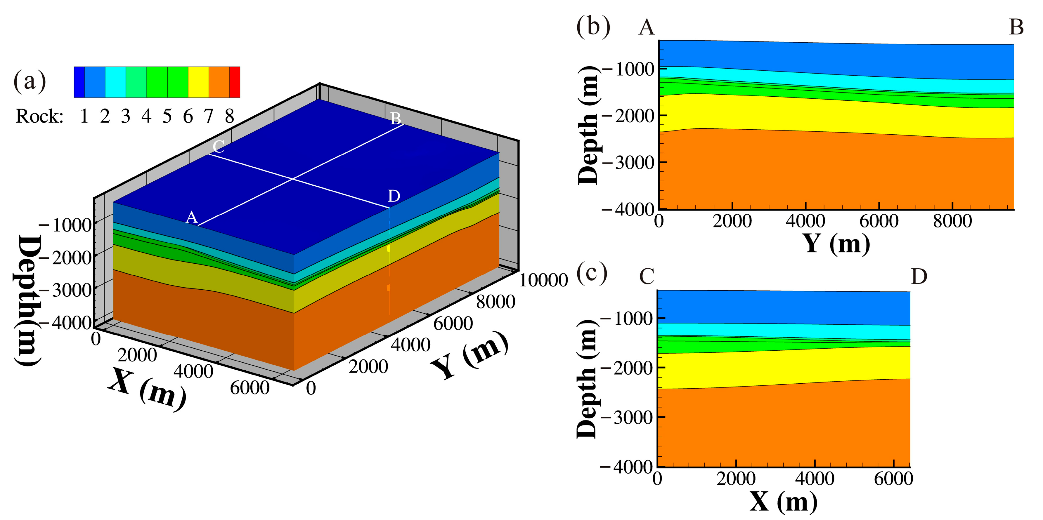
The geological model of the study area is developed by IGMESH [31], and the total area is approximately 62 km2 (Figure 1c). The maximum depth of the geological model is set to 4000 m. According to lithology information of nine wells, eight types of lithology are selected (Figure 2). The Kriging method is used to show variation in formation thickness, as shown in Figure 2.

3. Methods

3.1. Wellbore–Reservoir Coupled System

T2Well [21] integrates the flow and heat processes in both the wellbore and the reservoir, enabling the simulation of non-isothermal, multiphase, multicomponent flows in the deep wellbore–reservoir system. The fluid flow in the reservoir is described by Darcy’s law. The wellbore flow is described by a 1D momentum equation. Thermal conduction and convection can be considered in the wellbore–reservoir coupled system. In the leaking/feeding zone of the wellbore, the mass or energy inflow/outflow terms are calculated as in standard TOUGH2 (version 2.0) (i.e., the flow through the porous media) [32,33]. The HT processes between the wellbore and the reservoir are fully coupled. The specific governing equations are presented in the previous research [21,22,34].
An integrated finite difference scheme is employed, and the fluid flow and heat transport in the wellbore and reservoir coupled system can be described by the following equation:
M n κ , k + 1 M n κ , k Δ t = 1 V n m A n m F n m κ , k + 1 + V n q n κ , k + 1
where Δ t is time step size (s); M n κ , k (kg/m3, J/m3) represents κ component (water or energy) in the k th time step; V n is the volume of grid n (m3); A n m is the exchange area between grid n and m ; F n m κ , k + 1 is flux of fluid or energy (kg/m3, J/m3); and q n κ , k + 1 is the source/sink of fluid or energy in grid n .
Equation (1) is solved by Newton–Raphson iteration, and the residual terms can be expressed as follows:
R n κ = M n κ , k + 1 M n κ , k Δ t V n m A n m F n m κ , k + 1 + V n q n κ , k + 1 = 0
The chosen standard of the numerical convergence criterion is as follows:
R n k , k + 1 10 4
The adaptive time step is adopted, and the maximum time step depends on the specific conditions.

3.2. Inverse Modeling

In this paper, PEST (version 15) (Model-Independent Parameter Estimation) software [35] is employed to improve the efficiency of parameter identification in natural state modeling and history matching. Unlike a trial-and-error method, PEST can automatically call the HT model and conduct comparison between calculated values and measured values. The difference is described by the objective function. A Gauss–Marquardt–Levenberg optimization algorithm is used to accelerate the process of adjusting parameters. In the process of inverse modeling, the ranges of adjusting parameters and observed variables can be determined by users.

4. Numerical Modeling

4.1. Geothermal Background

The measured temperature data is shown in Figure 3. The temperature of the reservoir follows linear distribution and it is dominated by the upward conductive heat transfer.
Due to the difficulty of sampling, obtaining measurements of thermal parameters is not feasible; instead, these parameters are mostly estimated based on empirical values [36,37,38], as shown in Table 1. The dolomite reservoir of the Wumishan Formation has the characteristics of large karst crack and high thermal conductivity (higher than 2.93 W/m·°C), which facilitates HT activities in the reservoir. The Neogene sandstone and conglomerate have large porosity (from 0.25 to 0.40), and the thermal conductivity of rocks is higher than 1.68 W/m·°C. The porosity of the sandstone, sandy mudstone, and mudstone in the Quaternary and Neogene Systems is lower than 0.20, and the thermal conductivity generally varies from 0.84 to 2.00 W/m·°C, which restrains the thermal advective flow.
Above all, the geothermal reservoirs in Panzhuang Uplift belong to a conduction system [39] and have a similar genetic model to that of heat accumulation in sediment basins, i.e., a difference in thermal conductivity leads to heat re-distribution [26,40].

4.2. Natural State Model

The aim of establishing a natural state model is to identify the thermal conductivity distribution, which can be used to calculate the heat exchange between wellbore and the surrounding rock in the process of history matching. According to the previous research results [26], the heat transfer speed of the caprock with low heat conductivity is low, which leads to the high gradient of geothermal temperature. With the same heat flux, the bedrock usually has high heat conductivity and high heat transfer speed, which leads to the low temperature gradient; see Equation (4).
q = k · d T / d H
where q is heat flow (mW/m2); T is temperature (°C) and H is depth (m); dT/dH is geothermal gradient (°C/km); and the minus sign indicates heat flow transmitted from the interior earth towards the surface.
Here, 1D natural state model based on downhole logs in well CGSD-01 is established to obtain the thermal conductivity of geological layers. The adjusting ranges of thermal conductivity are presented in Table 2. In particular, the Wumishan Formation (Jxw) is divided into three groups (including Jxw-4, Jxw-3, and Jxw-2), with the same range of thermal conductivity in each.
The natural state model is discretized into 50 layers, and the thickness of each layer varies from 31.00 to 106.17 m. The depth of the model top reaches 44.38 m, which is below the constant temperature zone in Tianjin [16] (buried depth of 30 m, and temperature of 13.5 °C). According to the measured temperature logs and calculation results of hydrostatic pressure, the top of the model is regarded as the constant temperature (30.64 °C) and pressure (5.36 × 10⁵ Pa) boundaries. At the bottom of the model, a constant temperature boundary of 105 °C is used. To ensure the model can reach a steady state, the calculation time is set to 106 years.
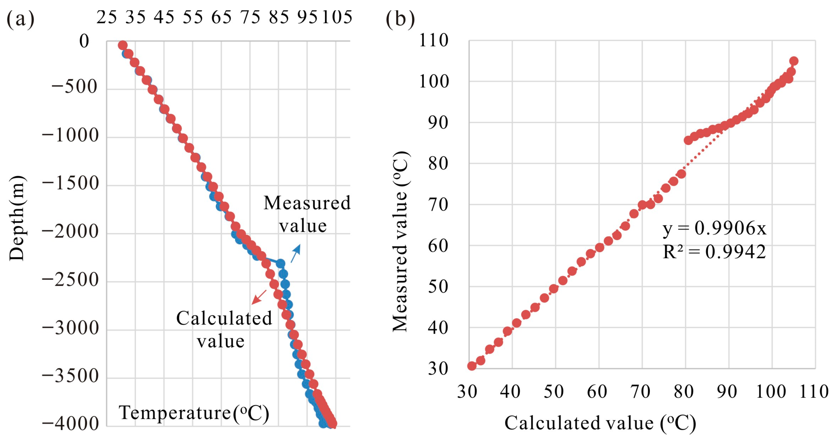
After 24 calls of the numerical model, the identification of thermal conductivity is complete (Table 2). The optimal values lie within the confidence interval, which suggests high reliability. The thermal conductivity of Q and Nm Formations plays an important role in heat re-distribution. There are 50 observation points included in the inverse modeling process and the root mean square error is 1.87 (Figure 4). The average residual error is −0.61, with a maximum value of 5.04 (at 2312 m depth) and a minimum value of −3.18 (at 3972 m depth). At a depth of between 2312 m and 2947 m, the calculated geothermal gradient is higher than the measured value, so the optimal thermal conductivity reaches the maximum value. In conclusion, the errors are acceptable, and the identified thermal conductivity can represent the real thermal properties of the formation.

4.3. History Matching of Pumping Test

4.3.1. Field Pumping Test Situation

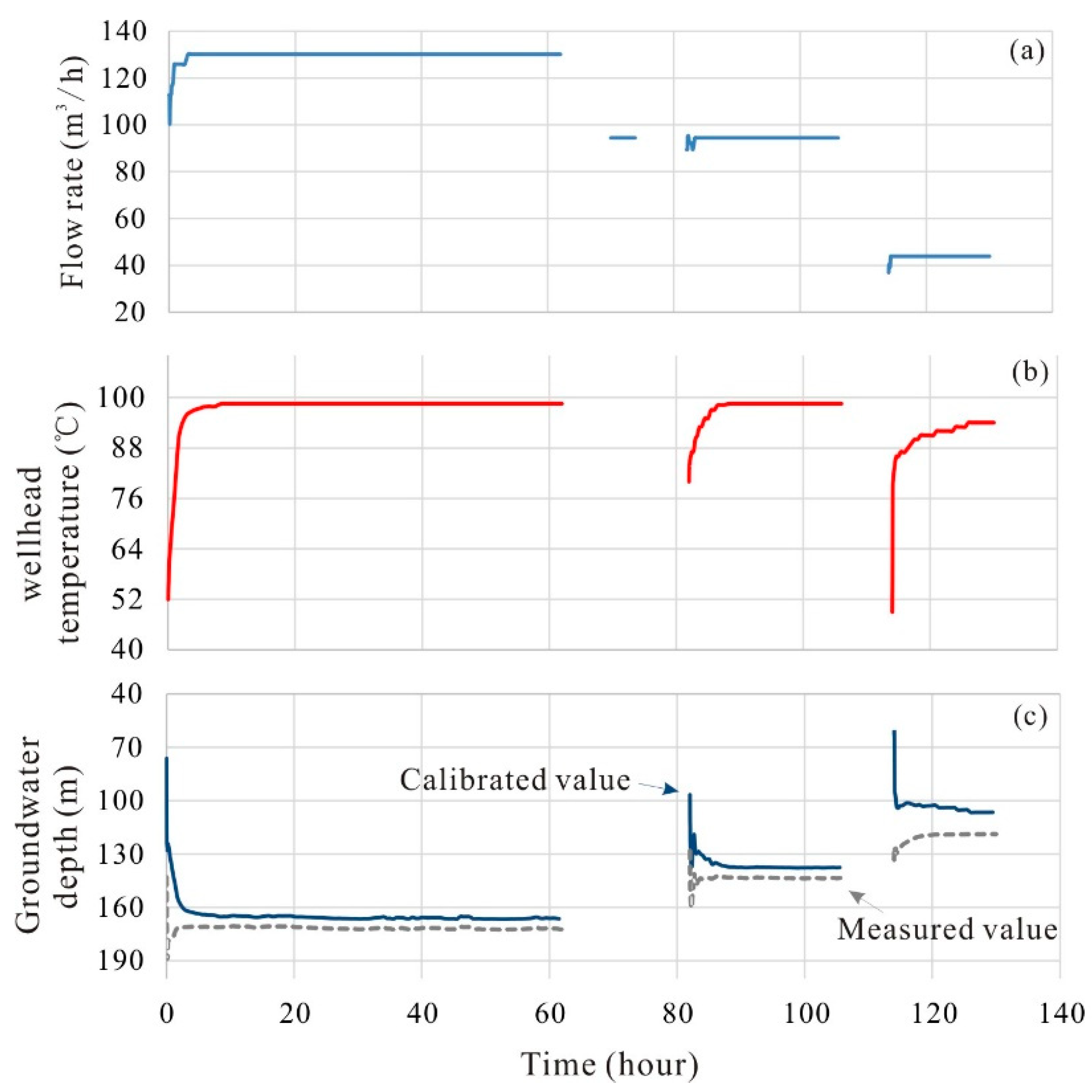
The pumping test interval of the well CGSD-01 ranged from 3715 m to 4051.68 m and the wellhead temperature and groundwater depth were recorded. The whole pumping test lasted for 138 h, consisting of three stages. In the large drawdown stage, it produced a flow rate of 130.2 m3/h for 62 h, and then 8 h of water-level recovery. In the middle drawdown stage, it produced a flow rate of 94.5 m3/h for 3 h and 50 min. However, due to the machine fault, there was 8 h of water-level recovery. Then, the official production lasted for 24 h, followed by an 8-h water-level recovery. In the small drawdown stage, it produced a flow rate of 43.9 m3/h for 16 h, followed by an 8-h water-level recovery. The specific observed variables are presented in Table 3 and Figure 5.
Since the density of water in the wellbore is temperature-dependent, a uniform temperature is adopted to calculate the calibrated groundwater depth, with Equation (5) applied for the calculation.
h = H ρ A [ H ( h 1 h 0 ) ] ρ S
where h is the calibrated groundwater depth (m); H is the depth of the reservoir (m); h1 is the observed groundwater depth (m); ρA is the average density of water in the wellbore (kg/m3); and ρS is the water density at the chosen uniform temperature (kg/m3).
According to wellhead temperature and bottom-hole temperature, ρA can be calculated. Given the linear temperature distribution of the reservoir, the average reservoir temperature of 102.6 °C is chosen as the uniform temperature and the corresponding ρS is about 956.411 kg/m3. The calibrated variation in groundwater depth with time is shown in Figure 5c.

4.3.2. History Matching of Temperatures and Pressures

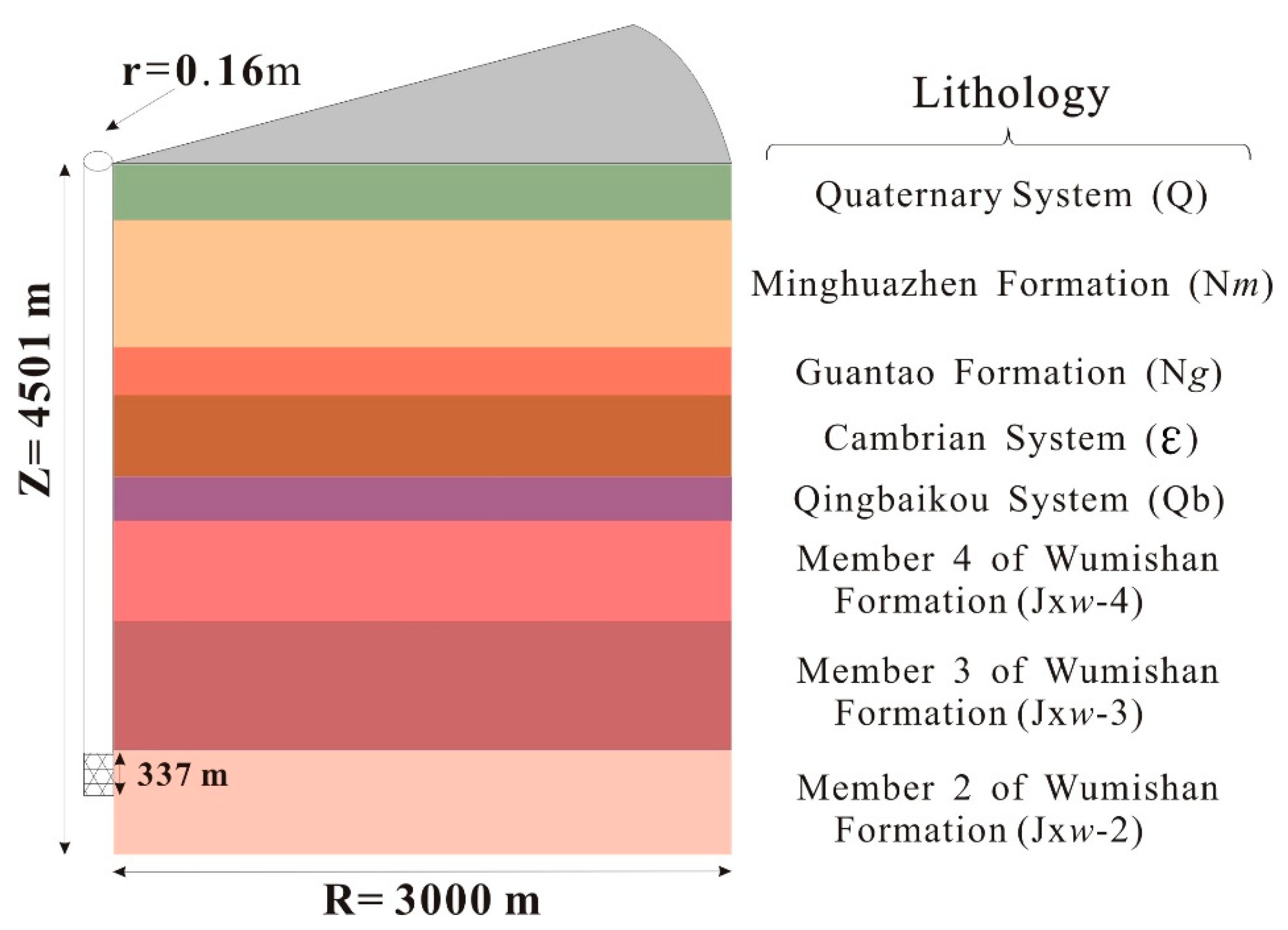
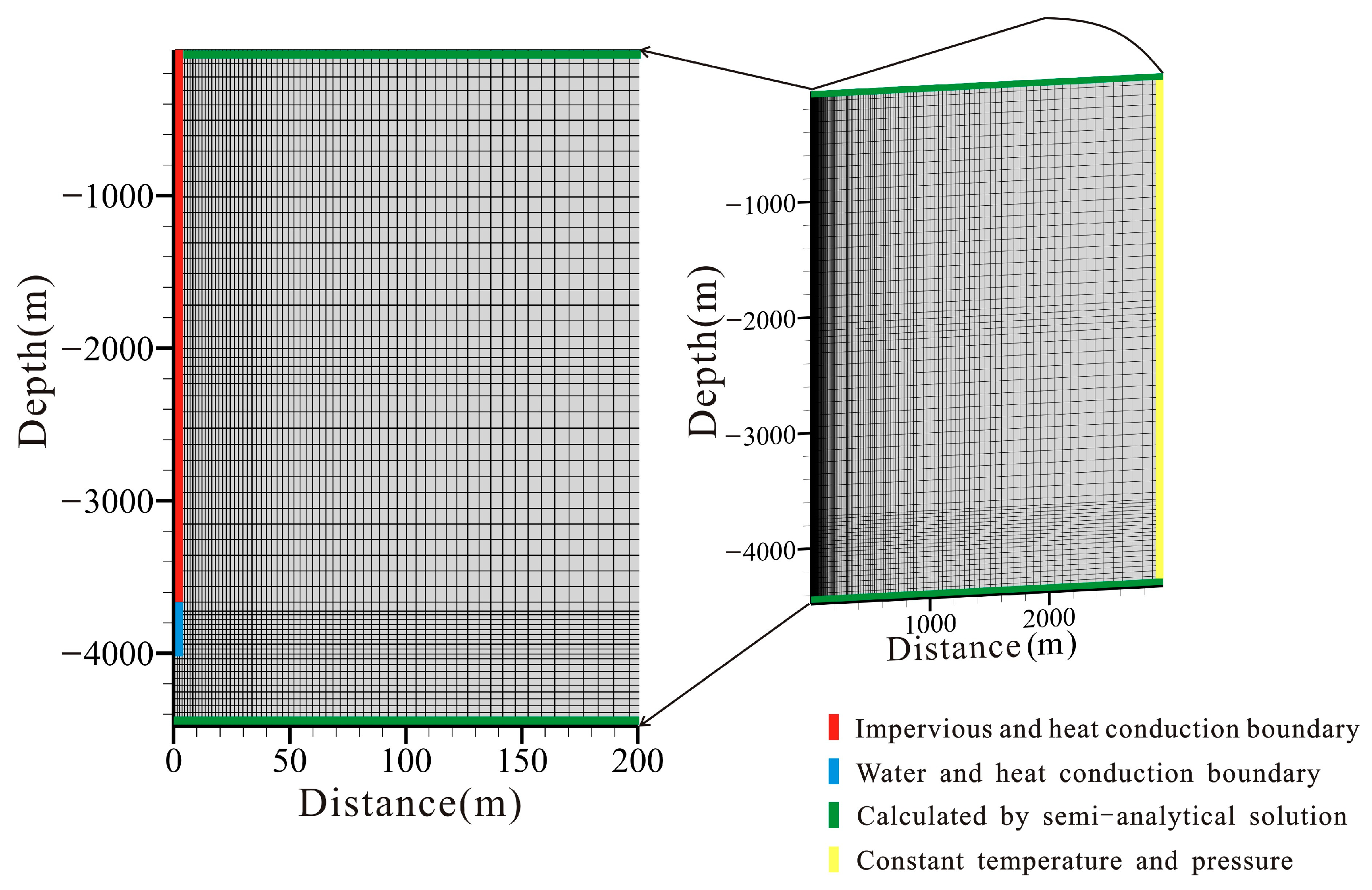
The borehole diameter is 0.16 m and a conceptual model is shown in Figure 6. To improve the calculation efficiency, the reservoir is discretized by radial 2D mesh and the wellbore is discretized by 1D mesh. Based on the vertical discretization of the natural state model, another 10 layers are added in the depth range of 4051.68~4501 m. Thus, there are 60 vertical layers, and the total distance in the horizontal direction (X) is 3 km, with a total 150 logarithmic intervals (Figure 7). The wellbore is divided into 50 grids. The total number of model grids is 9050.
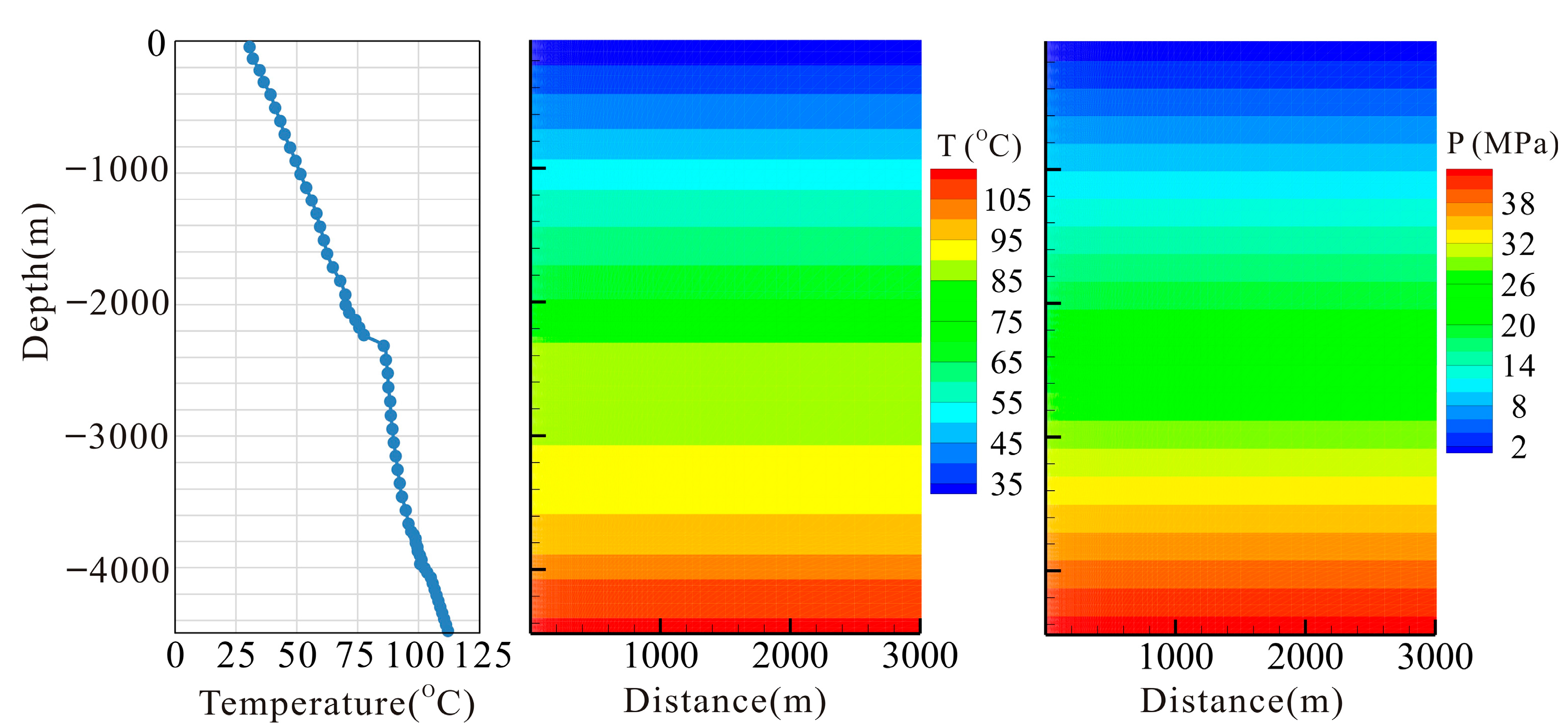
The measured temperature of the reservoir in the depth range of 0~4051.68 m is available, and the temperature of the reservoir deeper than 4051.68 m is calculated with a measured geothermal gradient of 1.73 °C/100 m (Figure 3). The initial temperature and hydrostatic pressure are shown in Figure 8. On the top and bottom of the history matching model, a semi-analytical method [41] is used in order to consider the heat exchange with confining beds. The lateral boundary is too far to influence the variation in temperature and pressure near the wellbore, so constant pressure and temperature boundary conditions are applied there.
The thermal conductivity of the surrounding rock refers to the calibrated value in the natural state model (Table 2), and the rest of the hydrothermal parameters are shown in Table 1. Based on the identified permeability of the Wumishan Formation in the previous research [36,37,38], the adjusting permeability varies from 3.65 × 10⁻¹⁴~3.65 × 10⁻¹¹ m2. Because the temperature profile is critical to heat exchange between the wellbore and the surrounding rock, the bottom temperature of the Radial 2D model (at the depth of 4501 m) is also considered in the inverse modeling process, in order to calibrate the bottom-hole temperature (at the depth of 4051.68 m). The variation in bottom temperature leads to the re-distribution of temperature and pressure logs of the steady state. Therefore, after update of permeability and bottom temperature, the model needs to be run towards the steady state, with a running time of 1 × 10⁶ years.
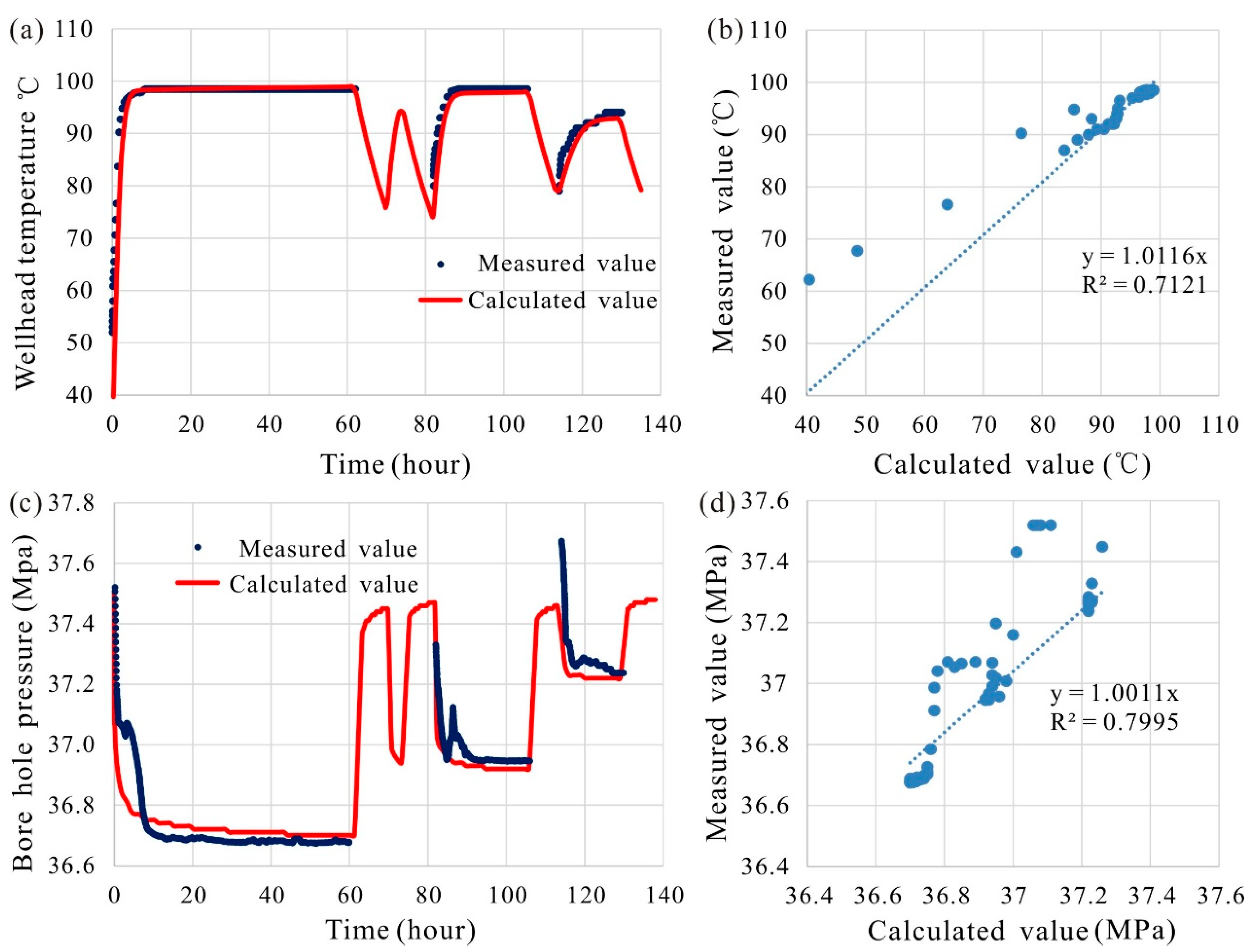
As shown in Figure 5, with the same dynamic conditions of flow rate for the entire pumping test, the comparison between the calibrated and observed value of temperature and groundwater depth is carried out. It is worth noting that pressure is used to describe variation in groundwater level in TOUGH2/T2Well, so it is necessary to convert the observed groundwater depth to pressure. The initial values and adjusting ranges of the permeability of the productive reservoir and the bottom temperature are shown in Table 4.
After 10 calls of the numerical model, the identification of permeability and bottom temperature was accomplished. According to the composite sensitivities of the adjusting parameters (Table 4), the permeability of the reservoir exerts a significant influence on the observed values (Figure 9c). A total of 210 observation points are incorporated into the inverse modeling. The Root Mean Square Error (RMSE) of temperature is 5.34 and the average residual error is 1.86. The rationale for the calculated value being lower than the initial measured temperature can be elucidated as follows. On the one hand, at the onset of the pumping test, the geothermal water from the deep reservoir mixes with the low-temperature geothermal water at the wellhead. On the other hand, the flow rate at the beginning is lower than that in the stable phase, which remarkably increases the heat exchange between the wellbore and the surrounding rock, thereby resulting in a low wellhead temperature. However, when the flow rate stabilizes, the wellhead temperature matches the measured value. Consequently, the errors of wellhead temperature at the very beginning of the pumping test in the wellbore–reservoir coupled model scarcely affect the wellhead temperature prediction during long-term stable operation. At the depth of 4051.68 m, the measured temperature (105 °C) is lower than the calibrated temperature (109 °C), indicating that the measured temperature logs may be affected by drilling fluids.
The RMSE of pressure is 0.12 and the average residual error is 0.04, with a maximum value of 0.46 and a minimum value of −0.05. At the onset of each drawdown test, the calculated pressure is slightly higher than the measured value. Generally, the borehole pressure (BHP) fits well with the measured value.
Above all, by the means of inverse modeling in the history matching model, the permeability of the productive reservoir and borehole temperature have been calibrated, which provides the basis of productivity optimization.

4.4. Geothermal Production Strategies and Criteria

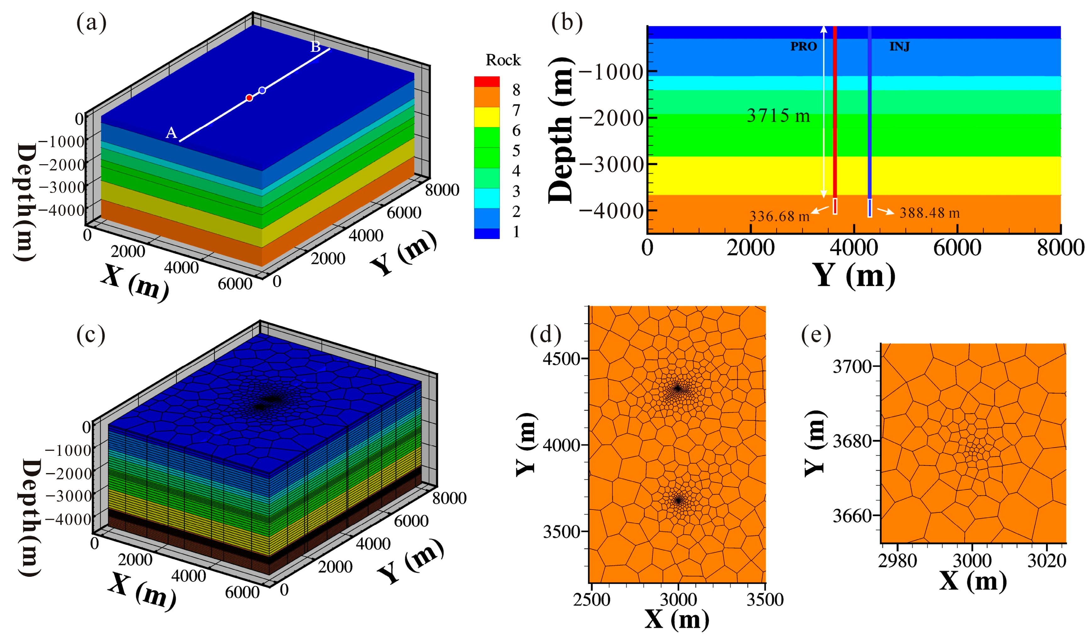
To prevent the groundwater level from declining even further, the geothermal doublet mode has been proposed in the Wumishan Formation of Panzhuang Uplift. Well CGSD-01 (with a depth of 4051.68 m) is used for production, and well CGSD-02 (with a depth of 4103.48 m) is utilized for injection. The depth of the perforated section of the production well ranges from 3715 to 4051.68 m, but the length of the perforated section of the injection well is unavailable. The well space of this geothermal doublet is 645 m. A 3D conceptual model with a domain size of 6000 m × 8000 m × 700 m is established (Figure 10).
According to the geological model of study area (Figure 2), the located formations are approximately horizontal. Therefore, the variation in formation thickness is not considered in the doublet model for productivity optimization. The vertical discretization is identical to that of the history matching model (60 layers), and local refinement of the mesh is achieved in the horizontal direction. The two wellbores are discretized in a 1D grid. The total number of grids of the doublet model is 56,021. The initial conditions and hydrothermal parameters are obtained from the natural state model and the history matching model (Figure 11). To account for the heat exchange between the reservoir and confining beds, a semi-analytical method [41] is employed at the top and bottom of the model. The boundaries in the horizontal direction are far from the target wells, so constant temperature and pressure boundary conditions are adopted.
The heating period in Tianjin is from 15 November to 15 March of the following year. The produced geothermal water during the heating period is allocated to every single day of the whole year to enhance the calculation efficiency of the numerical model and facilitate result analysis.
Energy analysis can be carried out through the calculation of the heat extract rate [32,42] (HER, MW) using the following equation:
H E R = Q p r o × h p r o Q i n j × h i n j
where Qpro is the flow rate of production (kg/s); Qinj is the flow rate of injection (kg/s); hpro is the specific enthalpy of the production fluid (kJ/kg); and hinj is the specific enthalpy of the injection fluid.
As is known, natural injection in a karst geothermal system is the most cost-effective strategy. But if a low permeability zone exists near the injection well, the injection pressure of the wellhead and the operational costs will increase significantly. Under such a condition, pressurizing injection is detrimental to the reservoir stability. The Input–Output Efficiency (IOE, MPa/°C) is proposed to evaluate the relationship between the injection costs and the geothermal system’s productivity. The lower the IOE of the karst geothermal system, the lower the injection costs and the higher the hydrothermal output.
I O E = P / T
where P is the BHP of the injection well and T is the variation in the wellhead temperature (°C).
The goal of the productivity optimization is to meet the heating demand of buildings with a total area of 1.33 × 10⁵ m2. When calculating the heating area, an average heating load of 45 W/m2 is selected for the North China region. To achieve productivity optimization, it is important to determine the specific range of engineering factors (including flow rate, perforated length of the injection well, and injection temperature) in the operation of a geothermal doublet. Generally, the flow rate of the geothermal doublet in Panzhuang Uplift ranges from 18,000 to 640,000 tons per year, equivalent to 40 to 220 m3/h. Because the maximum depth reaches 4103.48 m, the perforated length of the injection well may range from 50 to 360 m. The injection temperature in Tianjin ranges from 30 to 60 °C. The operational parameters of the designed geothermal doublet are summarized in Table 5, where the bold values represent the reference case simulation (RCS). In the process of productivity optimization, the impacts of engineering factors on production were evaluated, by means of a perturbation-based one-at-a-time approach [43].

4.5. Heterogeneity Implementation

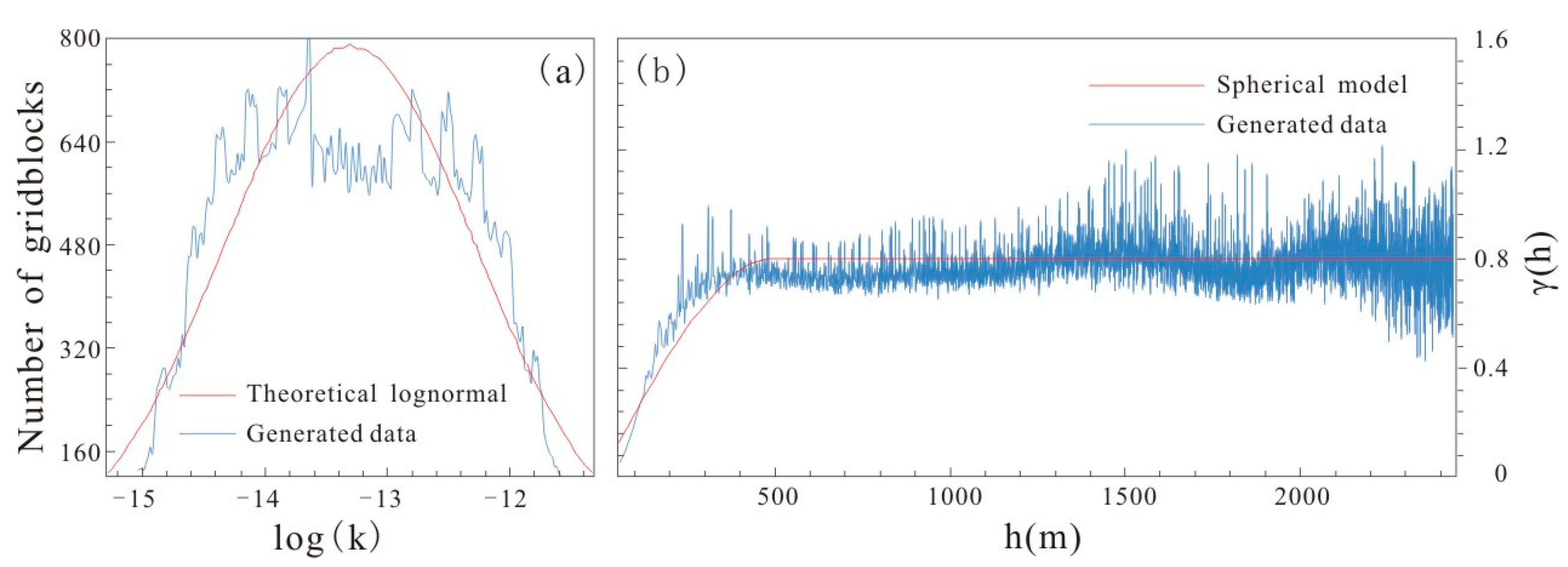
The structure and distribution of karst fractures can be characterized by porosity and permeability in the Equivalent Porosity Medium (EPM) [6,13] model, from a macro-average perspective. Therefore, porosity and permeability are regarded as the main variables to characterize heterogeneity. Considering that the HT processes basically occur near the wells, the heterogeneous subzone is defined as follows: (X = 2500~3500 m, Y = 3175~4825 m, and Z = −3700~−4525 m). The permeability is seen as a regionalized variable and the standard geostatistical techniques are applied. The subzone is discretized into 79,200 external cubic grids ( X = Y = Z = 25 m). The permeability of cubic grids follows a normal distribution [44,45], with an average permeability of 5.25 × 10⁻¹⁴ m2 and a variance of 0.8 (Figure 12). The spatial correlation among grids is governed by a spherical semivariogram [25]:
γ h = 1 2 × V a r Z x x + h = 1 2 × E × Z x x + h 2
γ h = 0 ,   h = 0 C o + C × 3 h 2 a h 3 2 a 3 C 0 + C ,   h a ,   0 < h a
where γ h is a spherical semivariogram, Z x is a regionalized variable, and h is the distance between spot x and another spot (m). V a r is the variance and E is the expectation. C o is the nugget effect ( C o = 0 ), the sill is 0.8, and C is arch height ( C = 0 ). a is spatial correlation length, and a = 500   m is selected.
Due to the discrepancy in the quantity of cubic grids and real grids, the calculated permeability is assigned to real grids (with the total number of 10,560) via Kriging interpolation. To determine the specific spatial distribution of porosity, a log-linear equation for porosity–permeability, established through regression analysis of logging interpretation results of wells DL-48 and DL-48B (Table 6, Figure 13), is utilized.
log k = 26.746 · φ 16.495
where correlation coefficient R2 is 0.8589.
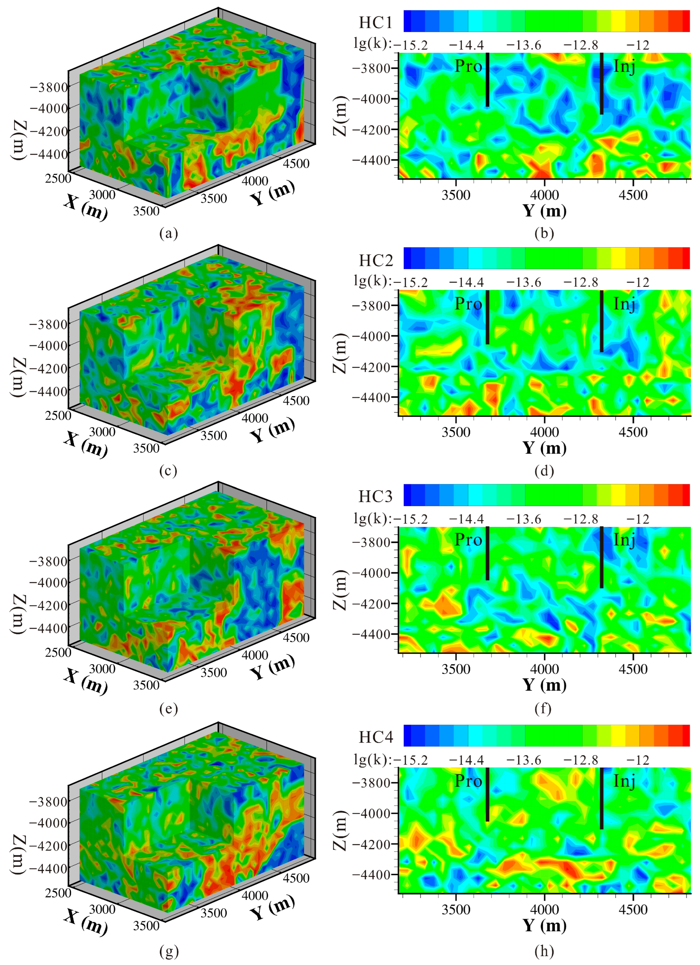
Four representative scenarios are selected and discussed (Figure 14):

5. Results and Discussion

5.1. Productivity Optimization

5.1.1. Flow Rate

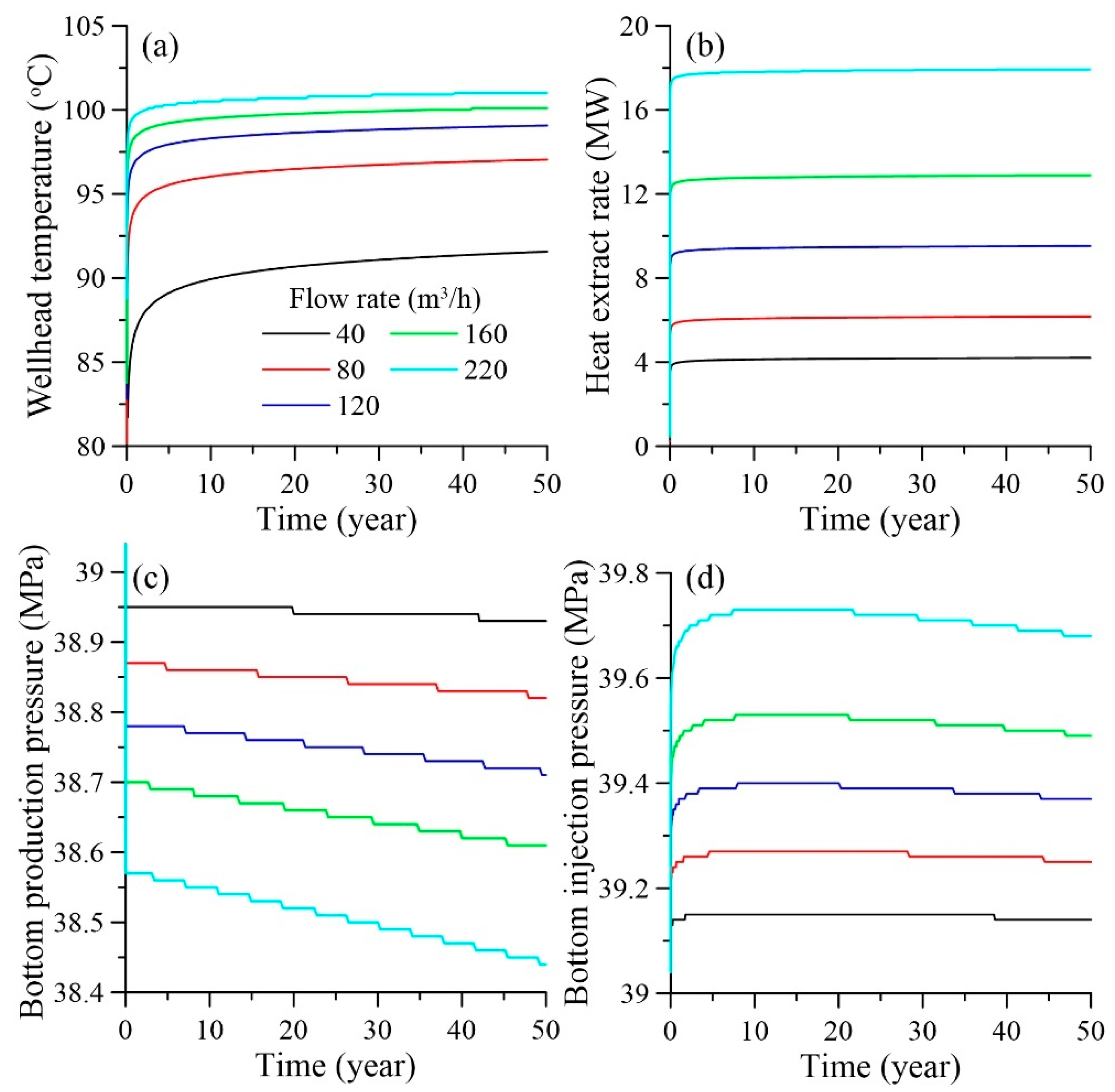
The geothermal production performance under flow rate ranging from 40 to 220 m3/h is demonstrated in Figure 15 and Figure 16. Unlike the geothermal production of a single well, forced convection induced by injection can drive more geothermal water from deeper sectors of the reservoir towards the production well, and wellhead temperature increases with time. For example, the wellhead temperature increases by 1.5 °C in 50 years, with a flow rate of 80 m3/h (Figure 15a). As the flow rate increases, the wellhead temperature increases accordingly. Under the flow rate of 80 m3/h and 220 m3/h, the wellhead temperature reaches 97.05 °C and 101 °C after 50 years (Figure 15a). This is because, as the flow rate increases, heat transfer between the wellbore and the surrounding rock has a diminished impact on the wellhead temperature, while forced convection near the production well is significantly enhanced.
As the flow rate increases, the HER increases, and no geothermal breakthrough occurs within a 50-year period (Figure 15b and Figure 16). The BHP of the injection well increases with the flow rate for the same operation time (Figure 15d). To calculate the IOE in the fiftieth year, the injection well BHP (39 MPa) and output temperature (91.57 °C) from the scenario with a flow rate of 40 m3/h are used as reference values. Among the scenarios with different flow rates in each group, the scenario with the flow rate of 80 m3/h corresponds to an HER of 6.17 MW, which can meet the heating demand of buildings with an area of 1.37 × 10⁵ m2 and achieve the production capacity target of this geothermal doublet project (target heating area: 1.33 × 10⁵ m2). The calculated IOE values for the scenario with flow rates of 80, 120, 160, or 220 m3/h are 0.046, 0.049, 0.057, and 0.072 MPa/°C, respectively, so the scenario with a flow rate of 80 m3/h yields the best economic benefit. Additionally, this flow rate is close to the typical geothermal production flow rate (200,000 tons per year) of geothermal production in Tianjin, China. After comprehensively considering geothermal productivity and reservoir stability, a flow rate of 80 m3/h is proposed as the optimal operating flow rate for this geothermal doublet.

5.1.2. Perforated Length of Injection Well

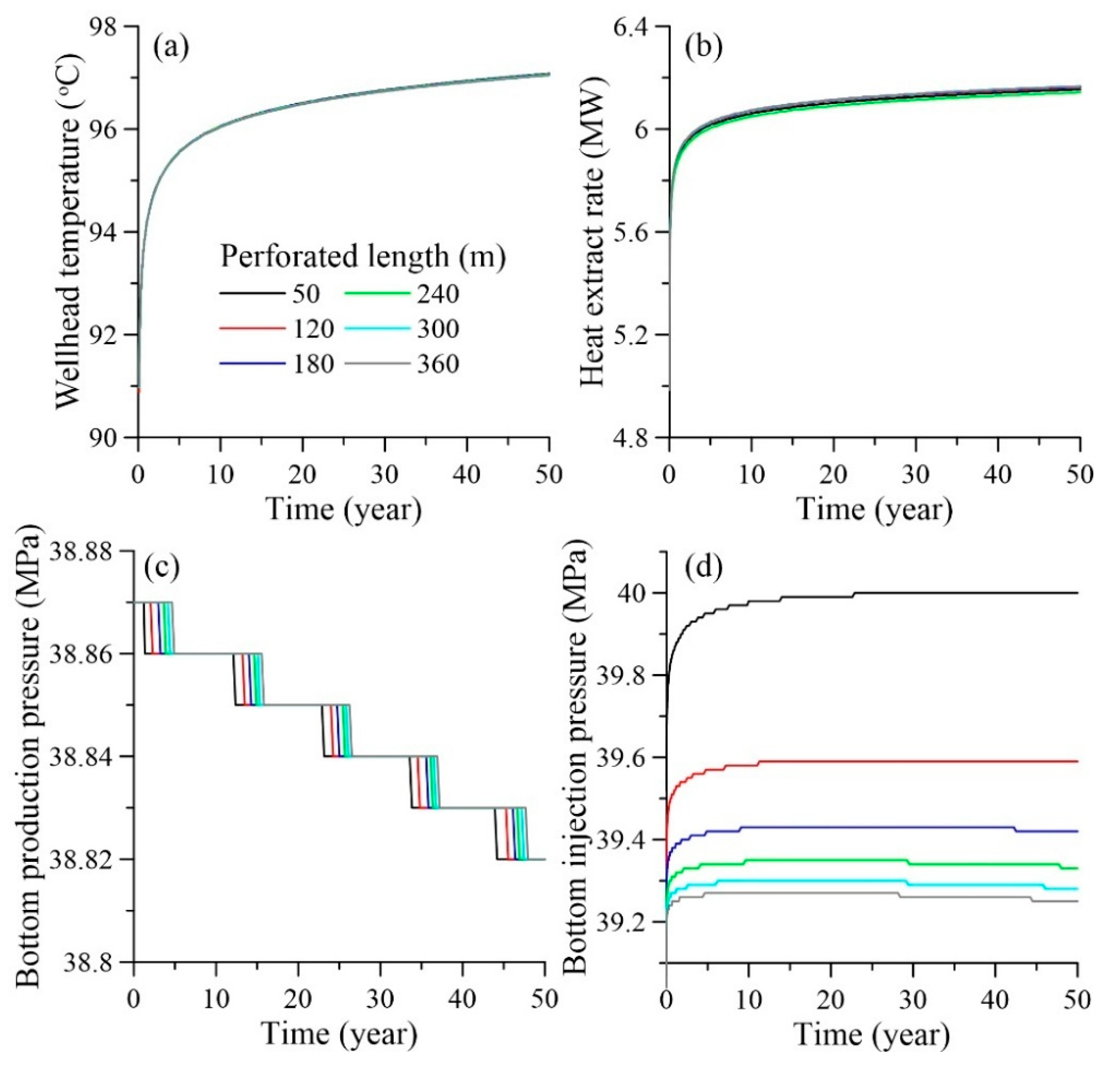
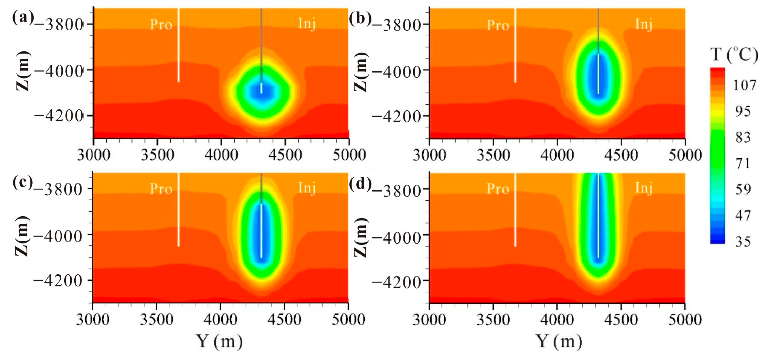
With the optimized flow rate of 80 m3/h, the geothermal production performance and reservoir temperature distribution of the reservoir under different injection depths are illustrated in Figure 17 and Figure 18. When the perforated length of the injection well (PLI) ranges from 50 to 180 m, injection water mainly migrates in the horizontal direction. However, limited by the flow rate, geothermal breakthrough never occurs (Figure 17a). When PLI ranges from 240 to 360 m, as the PLI increases, the vertical direction gradually becomes the main migration direction of injection water (Figure 18c,d). After 50 years, all the scenarios have the same BHP as the production well. Therefore, the variation in PLI has little influence on the BHP of the production well.
However, the BHP of the injection well is significantly affected by the PLI. When the PLI is 50 m, the BHP of the injection well reaches 40 MPa after 50 years (Figure 17d). Compared with the initial pressure (39 MPa), it increases by approximately 1 MPa. When the PLI is 360 m, the BHP of the injection well increases by only 0.25 MPa (Figure 17d). It can be concluded that an increase in the PLI facilitates the reinjection of geothermal tail water, which can effectively reduce the injection pressure and lower costs. A PLI varying from 360 to 388 m can effectively maintain the stability of hydrothermal production of this geothermal doublet.

5.1.3. Injection Temperature

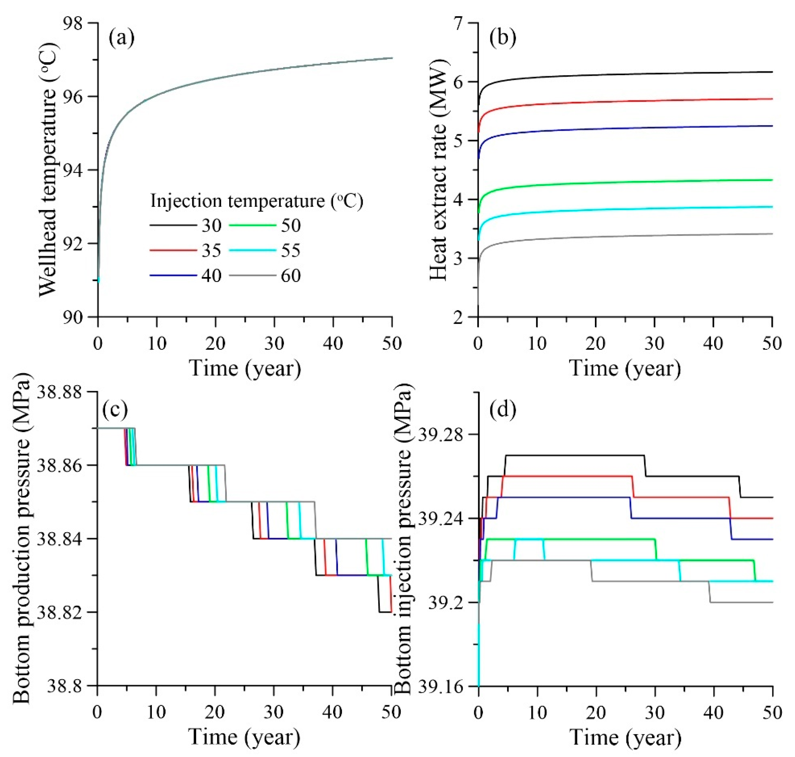
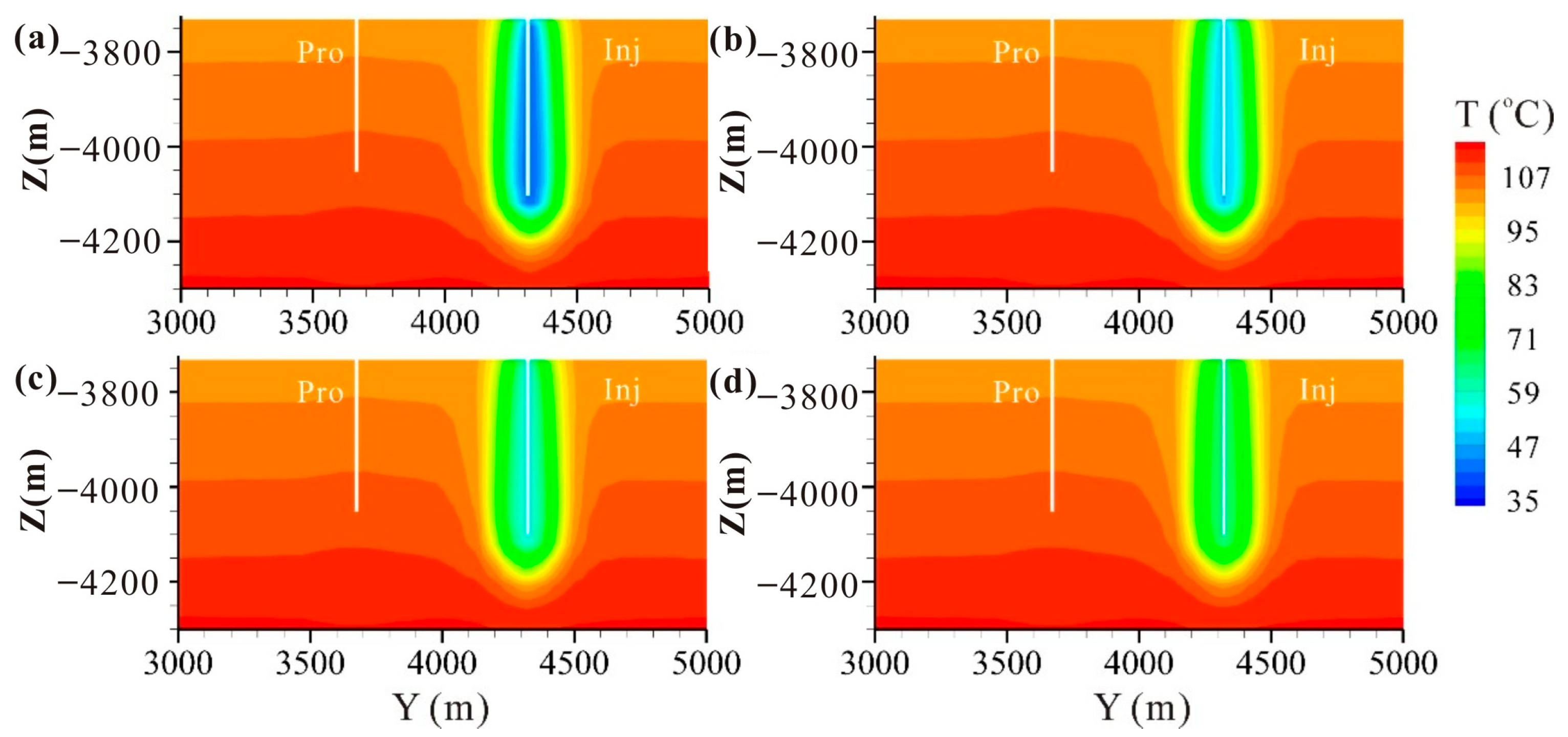
With the optimized PLI of 388 m, the relationship between geothermal productivity and injection temperature is summarized in Figure 19 and Figure 20. The injection of cold water can rapidly reduce the temperature of the reservoir around the injection well. With the decrease in injection temperature, the influence of cold water on the reservoir gradually expands (Figure 20). However, with the adopted flow rate and injection depth, the wellhead temperature is not affected by the injection operation over 50 years. The geothermal energy is extracted by a heat exchanger unit, so the HER increases as the injection temperature decreases (Figure 19b).
From the perspective of energy extraction, the scenario with the injection temperature of 30 °C has the maximum HER (6.17 MW), and its BHP of the injection well reaches 39.20 MPa in the 50th year (Figure 19b,d). With an injection temperature of 60 °C, the HER is 3.41 MW, and the BHP of the injection well is 39.25 MPa in the 50th year (Figure 19b,d). The pressure increase of 0.05 MPa almost doubles the HER. An injection temperature of 30 °C is recommended as the optimal temperature.
At this point, the optimization of hydrothermal production has been completed, and the optimal wellhead temperature is about 97 °C, with an HER of 6.17 MW. All the determined optimal parameters are going to be used in the risk evaluation of geothermal breakthrough.

5.2. Risk Evaluation of Geothermal Breakthrough

5.2.1. Homogeneous Reservoir

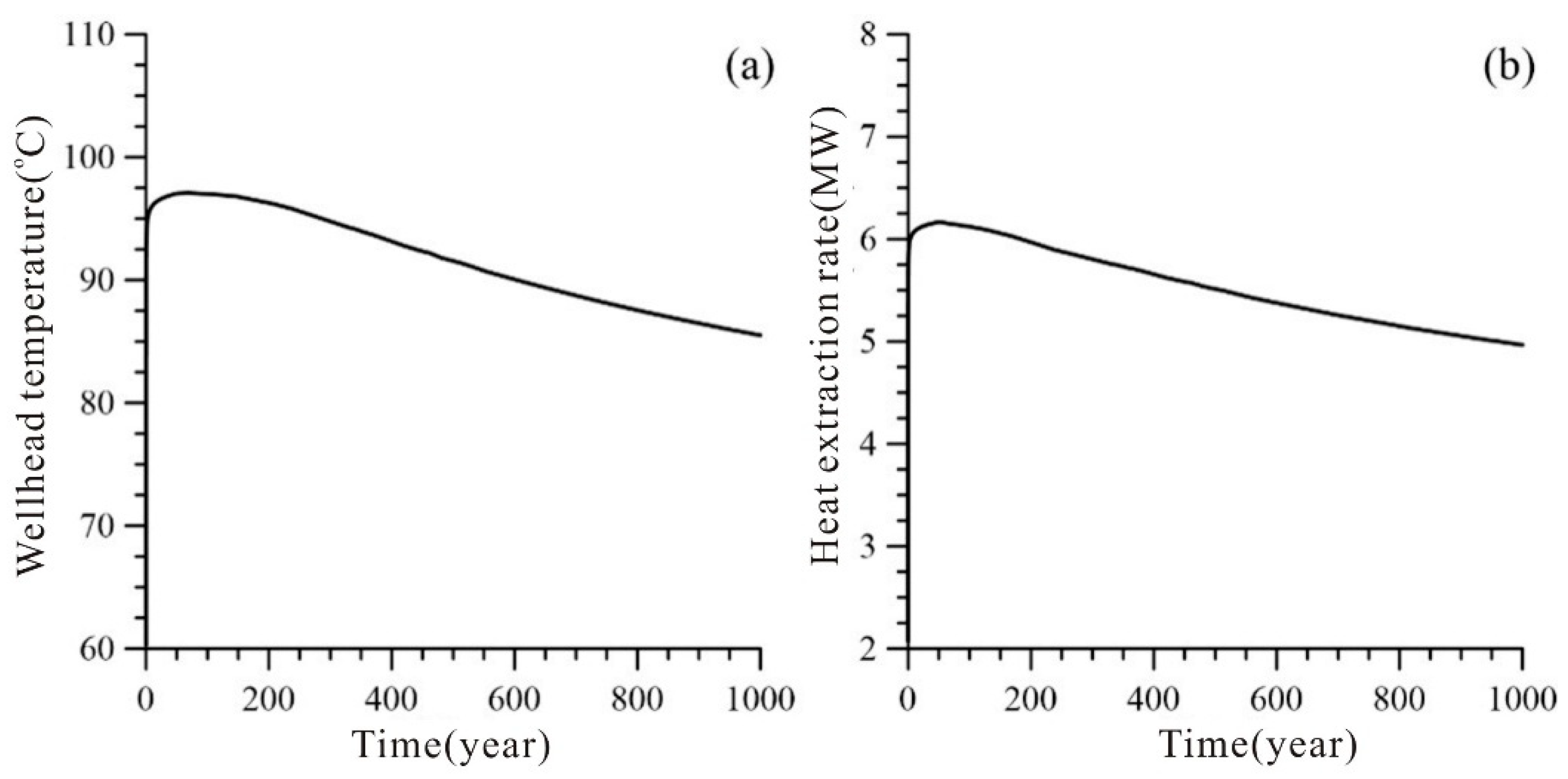
From the long-term benefits of project operation, it is necessary to evaluate the risk of geothermal breakthrough. If geothermal breakthrough occurs, cold water will migrate to the production well, which can significantly reduce the wellhead temperature. So, the simulation time of RCS has been prolonged to 1000 years. The results show that the wellhead temperature remains stable over 200 years, with a temperature reduction of 0.85 °C (Figure 21a) and an HER ranging from 4.97 to 6.17 MW (Figure 21b). After this geothermal doublet operates for 1000 years, the temperature reduction can reach 11.54 °C and the HER reduction can approach 1.2 MW. Therefore, with the condition of a homogeneous reservoir, this geothermal doublet can achieve stable operation for at least 200 years.

5.2.2. Heterogeneous Reservoir

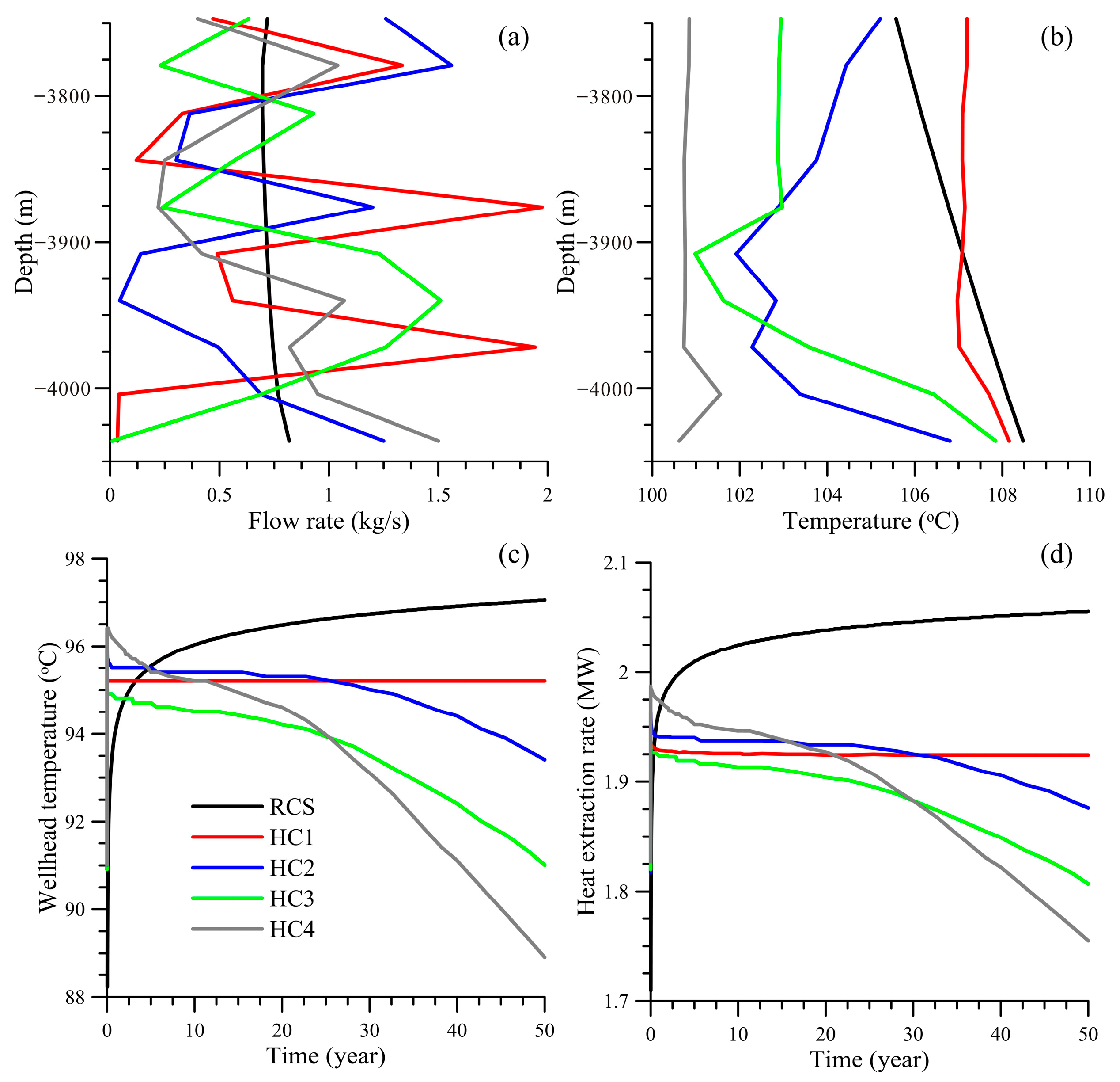
The flow rate distribution at the cross section of the production well and the reservoir is governed by the permeability distribution. In heterogeneous scenarios, the flow rate increases proportionally with the rise in permeability (Figure 22a). However, RCS exhibits nearly uniform flow rate along the open-hole section of the production well (Figure 22a). The HT processes triggered by injection exert a significant influence on the temperature distribution in the vicinity of the production well (Figure 22b). Therefore, the wellhead temperature is synergistically determined by flow rate and temperature distribution along the open-hole section of the production well.
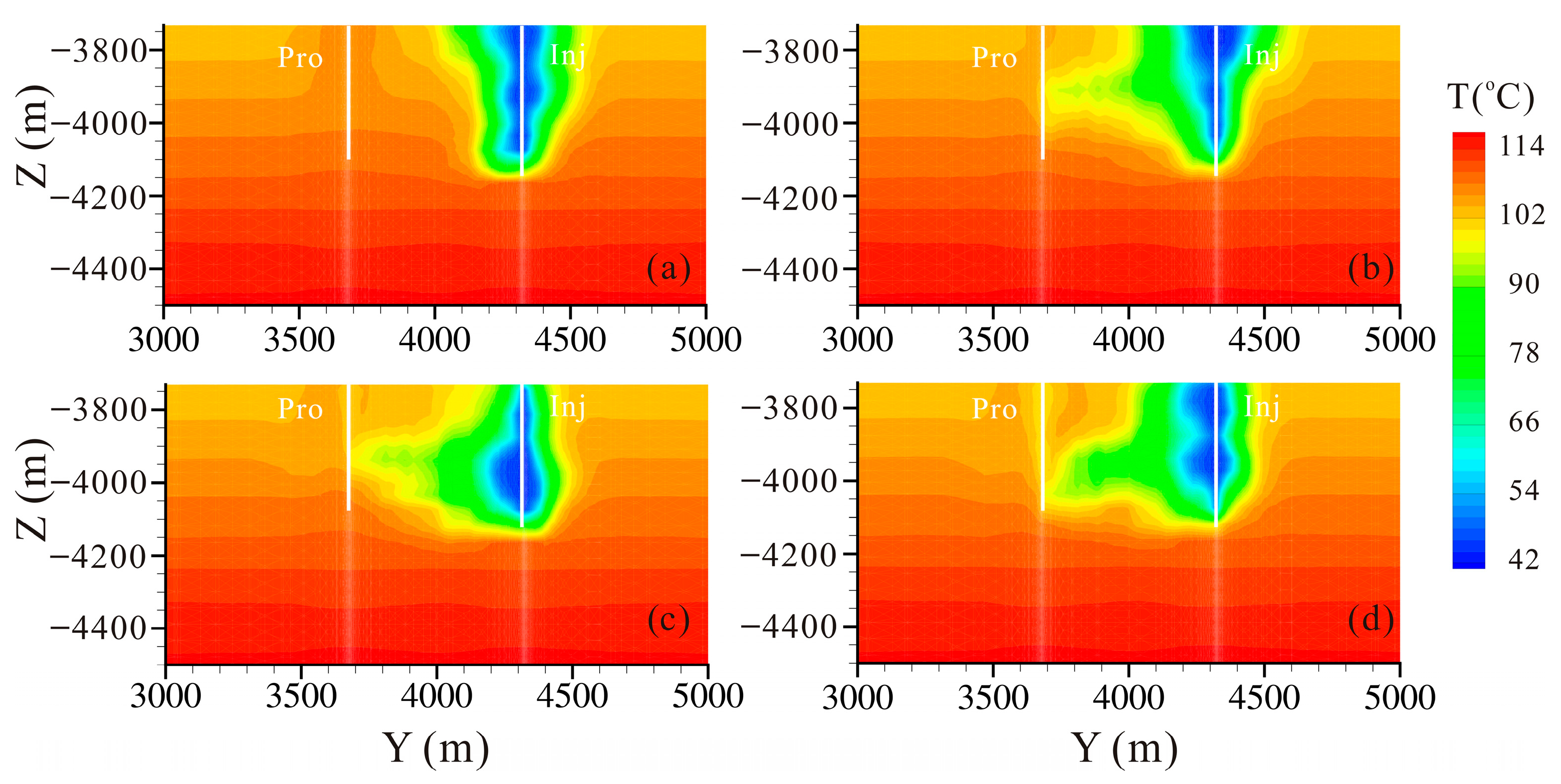
In scenario HC1, the low permeability zone is located around the injection well and the production well, which suppresses the horizontal migration of cold water, with no geothermal breakthrough. In the remaining heterogeneous scenarios (HC3~HC4), the existence of a high-permeability zone between wells facilitates the horizontal migration of cold water and induces geothermal breakthroughs to varying degrees. As shown in Figure 22c and Figure 23, the wellhead temperatures of HC2, HC3, and HC4 decrease by 2.5, 4, and 7.5 °C, respectively, within 50 years. The variation in HER with time shows a similar trend: the decreasing rate of HER for HC2, HC3, and HC4 is 4.1%, 6.7%, and 12%, respectively, within 50 years (Figure 22d). Considering heterogeneous factors, this geothermal doublet can only achieve stable operation for less than 25 years, with a flow rate of 80 m3/h.
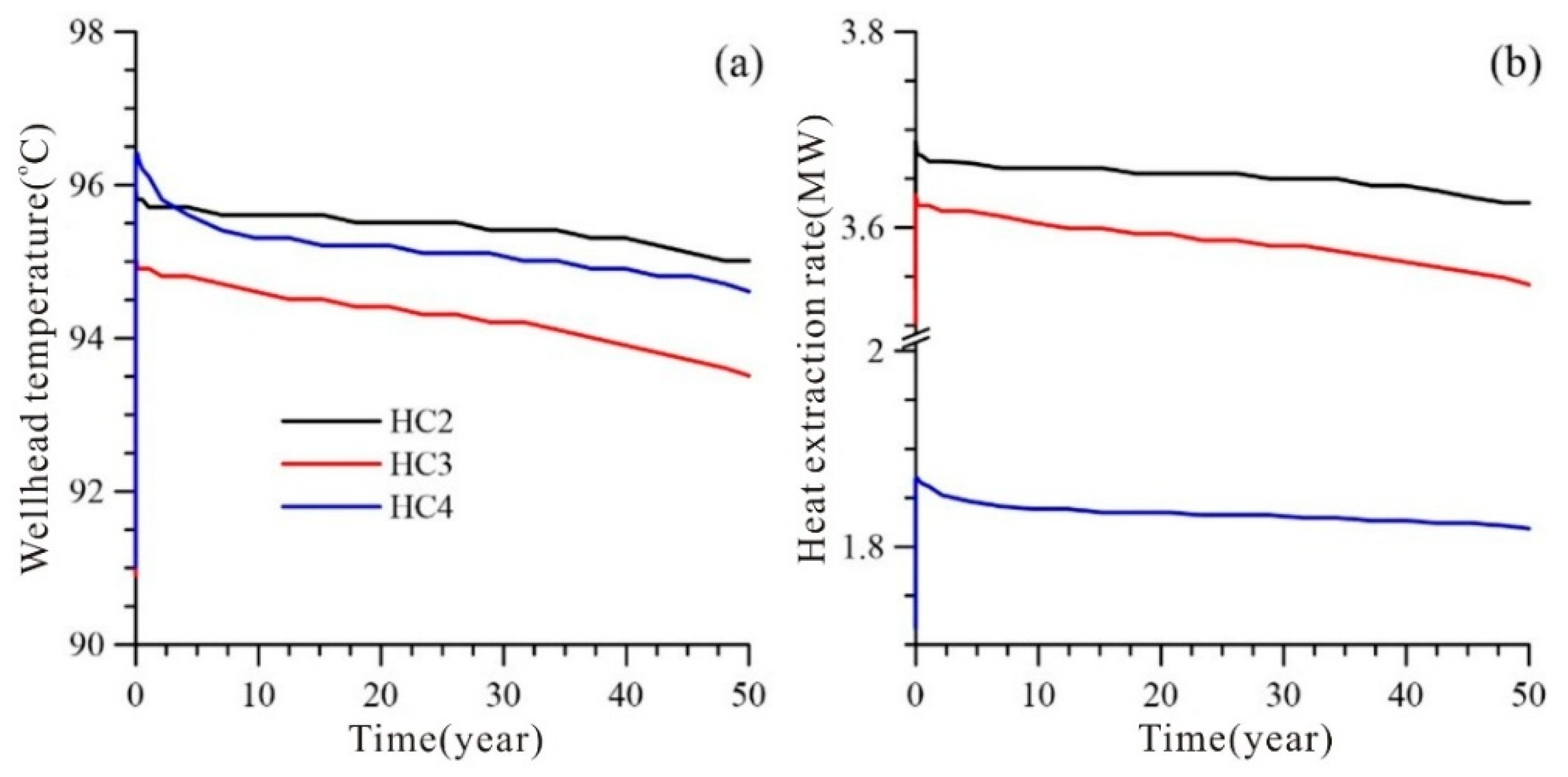
To reduce the risk of geothermal breakthrough, flow rate optimization of HC2, HC3, and HC4 have been conducted, with the flow rate ranging from 25 to 80 m3/h. The calculated results show that the reduction in wellhead temperature decreases with a decrease in flow rate (Figure 24a). A wellhead temperature reduction of less than 2 °C is adopted as the optimization criterion. The optimal flow rates of HC2, HC3, and HC4 are 50, 50, and 25 m3/h, respectively. In the 50th year, the wellhead temperature reduction in HC2, HC3, and HC4 is 0.9, 1.5, and 1.8 °C, respectively, (Figure 24a), with a decreasing rate of 0.94%, 1.6%, and 1.9%. Meanwhile, the HER reduction in HC2, HC3, and HC4 is 0.06, 0.09, and 0.03 MW, respectively, in the 50th year (Figure 24b), with a decreasing rate of 1.6%, 2.5%, and 1.6%. Overall, reducing the flow rate can mitigate the risk of geothermal breakthrough to a certain extent.

6. Conclusions

Based on the deep karst geothermal reservoir in Tianjin, China, an integrated wellbore–reservoir model was established. This model comprehensively incorporates non-Darcy flow in the wellbore, Darcy flow in the reservoir, and the HT processes within the wellbore–reservoir coupled system. The thermal conductivity of the surrounding rock was determined by natural state modeling. Additionally, inverse modeling was performed to calibrate the temperature profile and identify reservoir permeability in the process of history matching.
The identified parameters were used to establish a wellbore–reservoir coupled model for the field-scale geothermal doublet. Considering hydrothermal production and operation costs, a homogeneous model was constructed to sequentially optimize the flow rate, perforated length of the injection well, and injection temperature. Subsequently, both homogeneous and heterogeneous scenarios were analyzed to predict the hydrothermal production and evaluate the risk of geothermal breakthrough. The conclusions are drawn as follows:
(1)
The steady-state temperature profile is governed by borehole temperature and thermal conductivity. The geothermal gradient decreases with an increase in the thermal conductivity of the rock matrix and increases with a rise in borehole temperature. The results from natural state modeling show that the thermal conductivity of the Jxw Formation (2.93~4 W/m·°C) is higher than that of the Q (2.3 W/m·°C), Nm, and Ng Formations (2.5 W/m·°C).
(2)
The results of inverse modeling based on pumping tests show that the calibrated borehole (at a depth of 4051 m) temperature is 109 °C, which is 4 °C higher than the measured value (105 °C). Because geophysical well logging was conducted immediately after well completion of well CGSD-01, it is inferred that the measured values were affected by drilling fluid. The identified permeability of the Wumishan Formation of Panzhuang Uplift is 5.25 × 10⁻¹⁴ m2.
(3)
Taking the actual heating area (1.33 × 10⁵ m2) demand as the optimization objective, the engineering operation parameters of the geothermal doublet system under homogeneous reservoir conditions are adjusted. The optimization results are as follows: the optimal flow rate is 80 m3/h, the optimal perforated length of the injection well varies from 360 to 388 m, and the optimal injection temperature is 30 °C, with a wellhead temperature of 97 °C and a heat extraction rate of 6.17 MW.
(4)
From the perspective of the long-term benefit associated with project operation, the risk of geothermal breakthrough was comprehensively evaluated. In the case of only considering a homogeneous reservoir, this designed geothermal doublet can achieve stable operation for at least 200 years, with a temperature reduction of 0.85 °C and an HER ranging from 4.97 to 6.17 MW. Such results indicate that the geothermal doublet can provide a solid technical basis for the project’s long-term planning and risk management.
(5)
In the case of heterogeneous scenarios listed above, the high-permeability channels between wells can promote the occurrence of thermal breakthrough, thereby significantly reducing the stable operating flow rate of the geothermal doublet. Therefore, when optimizing well location layout, it is necessary to have a clearer understanding of the distribution characteristics of underground high-permeability channels.

Author Contributions

Conceptualization, F.L.; methodology, F.L.; software, X.Z.; validation, F.L.; formal analysis, F.L.; investigation, X.Z.; resources, X.G.; data curation, X.Z.; writing—original draft preparation, F.L.; writing—review and editing, X.G., Z.X. and H.C.; visualization, F.L.; supervision, X.G.; project administration, Z.X. and H.C.; funding acquisition, Z.X., X.G. and X.Z. All authors have read and agreed to the published version of the manuscript.

Funding

This research was funded by the Natural Resources Science and Technology Project, Department of Natural Resources of Zhejiang Province, grant number 2024ZJDZ024; the Second Batch of Doctor Innovation Stations in Southern Taihu Lake New District in 2024—Nuclear Industry Huzhou Survey, Planning Design and Research Institute Co., Ltd., grant number HKC202401; the Open Project Program of Key Laboratory of Groundwater Resources and Environment (Jilin University), Ministry of Education, grant number 202406ZDKF05; and the Natural Science Foundation of Heilongjiang Province, grant number LH2022D003.

Data Availability Statement

The data presented in this study are available on request from the corresponding author.

Conflicts of Interest

Fengyu Li and Xia Guo were employed by the Nuclear Industry Huzhou Survey Planning Design and Research Institute Co., Ltd. The remaining authors declare that the research was conducted in the absence of any commercial or financial relationships that could be construed as a potential conflict of interest.

References

  1. Rao, Y.; Wu, C.; He, Q. The antagonistic effect of urban growth pattern and shrinking cities on air quality: Based on the empirical analysis of 174 cities in China. Sustain. Cities Soc. 2023, 97, 104752. [Google Scholar] [CrossRef]
  2. Hou, J.; Cao, M.; Liu, P. Development and utilization of geothermal energy in China: Current practices and future strategies. Renew. Energy 2018, 125, 401–412. [Google Scholar] [CrossRef]
  3. Zhang, J.; Chen, L.; Sun, Y.; Xu, L.; Zhao, X.; Li, Q.; Zhang, D. Geothermal resource distribution and prospects for development and utilization in China. Natural Gas Ind. B 2024, 11, 6–18. [Google Scholar] [CrossRef]
  4. Yuan, Y.; Zhang, X.; Zhong, C.; Wang, Y.; Wen, D.G.; Xu, T.; Gherardi, F. Research Progress and Technical Challenges of Geothermal Energy Development from Hot Dry Rock: A Review. Energies 2025, 18, 1742. [Google Scholar] [CrossRef]
  5. Sun, C.S.; Shi, C.Y.; Zhu, Z.M.; Lin, H.X.; Li, Z.H.; Du, F.; Cao, Z.Z.; Lu, P.T.; Liu, L. Overburden failure characteristics and fracture evolution rule under repeated mining with multiple key strata control. Sci. Rep. 2025, 15, 28029. [Google Scholar] [CrossRef]
  6. Thomas, R. User’s Guide for Aquifer; Waterloo Hydrogeologic Incorporated: Waterloo, ON, Canada, 2007. [Google Scholar]
  7. Malama, B.; Kuhlman, K.L.; Barrash, W. Semi-analytical solution for flow in a leaky unconfined aquifer toward a partially penetrating pumping well. J. Hydrol. 2008, 356, 234–244. [Google Scholar] [CrossRef]
  8. Liu, G.; Wang, G.; Zhao, Z.; Ma, F. A new well pattern of cluster-layout for deep geothermal reservoirs: Case study from the Dezhou geothermal field, China. Renew. Energy 2020, 155, 484–499. [Google Scholar] [CrossRef]
  9. Zhao, Z.; Dou, Z.; Liu, G.; Chen, S.; Tan, X. Equivalent flow channel model for doublets in heterogeneous porous geothermal reservoirs. Renew. Energy 2021, 172, 100–111. [Google Scholar] [CrossRef]
  10. Teng, T.; Chen, Y.L.; Wang, S.; Jia, W.J.; Wang, Y.; Liu, K.; Li, Z.L. Water injection softening modeling of hard roof and application in Buertai coal mine. Environ. Earth Sci. 2025, 84, 54. [Google Scholar] [CrossRef]
  11. Li, S.T.; Wen, D.G.; Feng, B.; Li, F.Y.; Yue, D.D.; Zhang, Q.X.; Wang, J.Z.; Feng, Z.L. Numerical optimization of geothermal energy extraction from deep karst reservoir in North China. Renew. Energy 2023, 202, 1071–1085. [Google Scholar] [CrossRef]
  12. Jiang, X.; Li, F.Y.; Wang, Y.; Yuan, Y.J.; Li, R.R. Exploring the formation mechanism of cold mineral springs in the potassic basaltic region of Wudalianchi, Northeast China. Chem. Geol. 2025, 689, 122862. [Google Scholar] [CrossRef]
  13. Li, F.Y.; Guo, X.; Qi, X.F.; Feng, B.; Liu, J.; Xie, Y.P.; Gu, Y.M. A Surrogate Model-Based Optimization Approach for Geothermal Well-Doublet Placement Using a Regularized LSTM-CNN Model and Grey Wolf Optimizer. Sustainability 2025, 17, 266. [Google Scholar] [CrossRef]
  14. Wei, H.; Guo, X.; Zhang, H.K.; Feng, B.; Yuan, Y.L.; Li, F.Y.; Liu, J. A Simulation-Optimization Approach of Geothermal Well-Doublet Placement in North China Using Back Propagation Neural Network and Genetic Algorithm. Water 2025, 17, 911. [Google Scholar] [CrossRef]
  15. Wang, J.; Zhao, Z.; Liu, G.; Xu, H. A robust optimization approach of well placement for doublet in heterogeneous geothermal reservoirs using random forest technique and genetic algorithm. Energy 2022, 254, 124427. [Google Scholar] [CrossRef]
  16. Chen, J.F.; Zhao, Z.; Wang, J. A time-series forecasting model-based optimization approach for well-doublet system in geothermal reservoirs under geological uncertainty. Energy 2025, 330, 136926. [Google Scholar] [CrossRef]
  17. Chen, J.; Xu, T.; Liang, X.; Zhang, S. Evaluation and Optimization of Heat Extraction Strategies Based on Deep Neural Network in the Enhanced Geothermal System. J. Energy Eng. 2022, 149, 04022050. [Google Scholar] [CrossRef]
  18. Liu, G.; Zhao, Z.; Xu, H.; Zhang, J.; Kong, X.; Yuan, L. A robust assessment method of recoverable geothermal energy considering optimal development parameters. Renew. Energy 2022, 201, 426–440. [Google Scholar] [CrossRef]
  19. Hamm, V.; Bouzit, M.; Lopez, S. Assessment of complex well architecture performance for geothermal exploitation of the Paris basin: A modeling and economic analysis. Geothermics 2016, 64, 300–313. [Google Scholar] [CrossRef]
  20. Wang, J.; Tan, X.; Zhao, Z.; Chen, J.; He, J.; Shi, Q. Coupled thermo-hydro-mechanical modeling on geothermal doublet subject to seasonal exploitation and storage. Energy 2024, 293, 130650. [Google Scholar] [CrossRef]
  21. Pan, L.; Oldenburg, C.M. T2Well-An integrated wellbore-reservoir simulator. Comput. Geosci. 2014, 65, 46–55. [Google Scholar] [CrossRef]
  22. Xu, T.F.; Li, F.Y.; Feng, B.; Feng, G.H.; Jiang, Z.J. Numerical evaluation of the performance of a single-well groundwater source heat pump system in Beijing, China. Energy Explor. Exploit. 2020, 38, 201–221. [Google Scholar] [CrossRef]
  23. Xu, T.; HU, Z.; Feng, B.; Li, F.Y.; Jiang, Z.J. Numerical evaluation of building heating potential from a coaxial closed-loop geothermal system using wellbore-reservoir coupling numerical model. Energy Explor. Exploit. 2020, 38, 733–754. [Google Scholar] [CrossRef]
  24. HU, Z.; Xu, T.F.; Feng, B.; Yuan, Y.L.; Li, F.Y.; Feng, G.H.; Jiang, Z.J. Thermal and fluid processes in a closed-loop geothermal system using CO2 as a working fluid. Renew. Energy 2020, 154, 351–367. [Google Scholar] [CrossRef]
  25. Feng, G.; Xu, T.; Gherardi, F.; Jiang, Z.; Bellani, S. Geothermal assessment of the Pisa plain, Italy: Coupled thermal and hydraulic modeling. Renew. Energy 2017, 111, 416–427. [Google Scholar] [CrossRef]
  26. Li, F.Y.; Xu, T.; Li, S.; Feng, B.; Jia, X.; Feng, G.H.; Zhu, H.; Jiang, Z.J. Assessment of Energy Production in the Deep Carbonate Geothermal Reservoir by Wellbore-Reservoir Integrated Fluid and Heat Transport Modeling. Geofluids 2019, 2019, 8573182. [Google Scholar] [CrossRef]
  27. Yu, H.; Xu, T.; Yuan, Y.; Gherardi, F.; Feng, B.; Jiang, Z.J.; Hu, Z. Enhanced heat extraction for deep borehole heat exchanger through the jet grouting method using high thermal conductivity material. Renew. Energy 2021, 177, 1102–1115. [Google Scholar] [CrossRef]
  28. Yu, H.; Xu, T.; Yuan, Y.; Feng, B.; ShangGuan, S. Enhanced heat extraction performance from deep buried U-shaped well using the high-pressure jet grouting technology. Renew. Energy 2023, 202, 1377–1386. [Google Scholar] [CrossRef]
  29. Yu, H.; Xu, T.; Yuan, Y.; Gherardi, F.; Tian, H.L. Single well geothermal heating systems: Technical and economic assessment of two widely-used configurations. J. Hydrol. 2024, 635, 131126. [Google Scholar] [CrossRef]
  30. Chen, H.; Song, Z.; He, G.; Li, S.; Xu, B.; Ma, H.; Du, Y.; Yin, G. Application of muti-process combined well flushing and pumping test in well CGSD-01. Explor. Eng. Rock Soil Drill. Tunneling 2019, 46, 8–13. (In Chinese) [Google Scholar]
  31. Hu, L.T.; Zhang, K.N.; Cao, X.Y.; Li, Y.; Guo, C.B. IGMESH: A convenient irregular-grid-based pre- and post-processing tool for TOUGH2 simulator. Comput. Geosci. 2016, 95, 11–17. [Google Scholar] [CrossRef]
  32. Pruess, K.; Oldenburg, C.M.; Moridis, G.J. TOUGH2 User’s Guide Version 2; Office of Scientific & Technical Information Technical Reports; Office of Scientific & Technical Information: Oak Ridge, TN, USA, 1999. [Google Scholar]
  33. Yu, H.; Xu, T.; Yuan, Y.; Gherardi, F.; Tian, H.L. Numerical analysis of coupled thermal-hydraulic processes based on the embedded discrete fracture modeling method. Appl. Therm. Eng. 2024, 253, 123765. [Google Scholar] [CrossRef]
  34. Zhong, C.; Xu, T.; Gherardi, F.; Yuan, Y. Comparison of CO2 and water as working fluids for an enhanced geothermal system in the Gonghe Basin, northwest China. Gondwana Res. 2023, 122, 199–214. [Google Scholar] [CrossRef]
  35. Doherty, J.E. PEST: Model Independent Parameter Estimation; Watermark Computing: Corinda, Australia, 2008. [Google Scholar]
  36. Lin, L. Sustainable Development and Utilization of Thermal Groundwater Resources in the Geothermal Reservoir of the Wumishan Group in Tianjin. Ph.D. Thesis, China University of Geosciences, Beijing, China, 2006. (In Chinese). [Google Scholar]
  37. Tian, G. Sustainable Development and Utilization of Geothermal Resources in the Donglihu Hot Spring Resort of Tianjin. Ph.D. Thesis, China University of Geosciences, Beijing, China, 2014. (In Chinese). [Google Scholar]
  38. Peng, Z. Geothermal Reinjection Numerical Simulation and Resource Evaluation of the Wumishan Group in Dongli District of Tianjin. Ph.D. Thesis, China University of Geosciences, Beijing, China, 2016. (In Chinese). [Google Scholar]
  39. Jiang, Z.J.; Xu, T.; Wang, Y. Enhancing heat production by managing heat and water flow in confined geothermal aquifers. Renew. Energy 2019, 142, 684–694. [Google Scholar] [CrossRef]
  40. Pang, Z.; Pang, J.; Kong, Y.; Luo, L.; Duan, Z.; Yang, F.; Wang, S. Large Karstic Geothermal Reservoirs in Sedimentary Basins in China: Genesis, Energy Potential and Optimal Exploitation. In Proceedings of the World Geothermal Congress (WGC-2015), Melbourne, Australia, 16–24 April 2015. [Google Scholar]
  41. Vinsome, P.K.W.; Westerveld, J. A simple method for predicting cap and base rock heat losses in thermal reservoir simulators. J. Can. Pet. Tech. 1980, 19, 87–90. [Google Scholar] [CrossRef]
  42. Xu, T.F.; Yuan, Y.L.; Jia, X.F.; Lei, Y.D.; Li, S.T.; Feng, B.; Hou, Z.Y.; Jiang, Z.J. Prospects of power generation from an enhanced geothermal system by water circulation through two horizontal wells: A case study in the Gonghe Basin, Qinghai Province, China. Energy 2018, 148, 196–207. [Google Scholar] [CrossRef]
  43. Saltelli, A.; Ratto, M.; Andres, T.; Campolongo, F.; Cariboni, J.; Gatelli, D.; Saisana, M.; Tarantola, S. Global Sensitivity Analysis. The Primer; John Wiley & Sons, Ltd.: Hoboken, NJ, USA, 2008; p. 297. [Google Scholar]
  44. Tian, H.L.; Pan, F.; Xu, T.; McPherson, B.J.; Yue, G.; Mandalaparty, P. Impacts of hydrological heterogeneities on caprock mineral alteration and containment of CO2 in geological storage sites. Int. J. Greenh. Gas Control 2014, 24, 30–42. [Google Scholar] [CrossRef]
  45. Xu, H.; Cheng, J.; Zhao, Z.; Lin, T.; Liu, G.; Chen, S. Coupled thermo-hydro-mechanical-chemical modeling on acid fracturing in carbonatite geothermal reservoirs containing a heterogeneous fracture. Renew. Energy 2021, 172, 145–157. [Google Scholar] [CrossRef]
Figure 1. (a) Location of Panzhuang geothermal field, Tianjin, China. (b) Stratigraphy of well CGSD-01. (c) The well location in the model domain.
Water 17 03269 g001
Figure 2. Lithology structure of the study area (rectangular area of the dotted line in Figure 1c) (1: Quaternary System; 2: Minghuazhen Formation; 3: Guantao Formation; 4: Cretaceous Formation; 5: Ordovician System; 6: Cambrian System; 7: Qingbaikou System; 8: Wumishan Formation). (a) 3D lithology structure of the study area; (b) lithology structure of the A-B cross section; (c) lithology structure of the C-D cross section.
Water 17 03269 g002
Figure 3. Temperature profile of well CGSD-01. (Q: Quaternary System; Nm: Minghuazhen Formation of Neogene System; Ng: Guantao Formation of Neogene System; ε: Cambrian System; O: Ordovician System; Qb: Qingbaikou System; Jxw: Wumishan Formation of Jixian System).
Water 17 03269 g003
Figure 4. (a) Temperature logs; red dot represents calculated value and blue dot represents measured value. (b) Root mean square error analysis; R is correlation coefficient.
Water 17 03269 g004
Figure 5. Flow rate (a), wellhead temperature (b), and groundwater depth (c) variations with time during the pumping test of well CGSD-01.
Water 17 03269 g005
Figure 6. Conceptual model of wellbore–reservoir coupled system in the site-scale pumping test.
Water 17 03269 g006
Figure 7. The radial 2D mesh space discretization and specific boundary conditions.
Water 17 03269 g007
Figure 8. Initial temperature and pressure conditions in the history matching model.
Water 17 03269 g008
Figure 9. The comparison results between the calculated value and the measured value in the history matching model. Wellhead temperature (a) and borehole pressure (c) variation with time; RMSE analysis of wellhead temperature (b) and bore hole pressure (d); R2 (correlation coefficient) is the correlation coefficient.
Water 17 03269 g009
Figure 10. (a) Conceptual model of the geothermal doublet; (b) lateral 2D cross section of the model (X = 3000 m), where the red solid line represents the production well and the blue solid line represents the injection well; (c) discretization of the model; (d,e) mesh refinement near the wells.
Water 17 03269 g010
Figure 11. The calibrated temperature (a) and pressure (b) profiles of well CGSD-01.
Water 17 03269 g011
Figure 12. (a) Lognormal distribution of permeability. (b) Spherical semivariogram model.
Water 17 03269 g012
Figure 13. The log-linear porosity–permeability relationship in the Wumishan Formation of Panzhuang Uplift. Black dots represent the interpretation results of well DL-48 and the related data are provided in Table 6. Red dots represent the interpretation results of well DL-48B from the previous research [26].
Water 17 03269 g013
Figure 14. The permeability distribution of HC1, HC2, HC3, and HC4. “Pro” represents the production well and “Inj” represents the injection well. (a) 3D permeability distribution of HC1; (b) 2D permeability cross section between wells for HC1, with low permeability between the two wells; (c) 3D permeability distribution of HC2; (d) 2D permeability cross section between wells for HC2, with high permeability between the two wells; (e) 3D permeability distribution of HC3; (f) 2D permeability cross section between wells for HC3, with high permeability at the top of the reservoir and low permeability at the bottom of the reservoir; (g) 3D permeability distribution of HC4; (h) 2D permeability cross section between wells for HC4, with high permeability between the two wells and low permeability at the bottom of each well.
Water 17 03269 g014
Figure 15. Variations in wellhead temperature (a), HER (b), bottom production pressure (c), and bottom injection pressure (d) with time under different flow rates.
Water 17 03269 g015
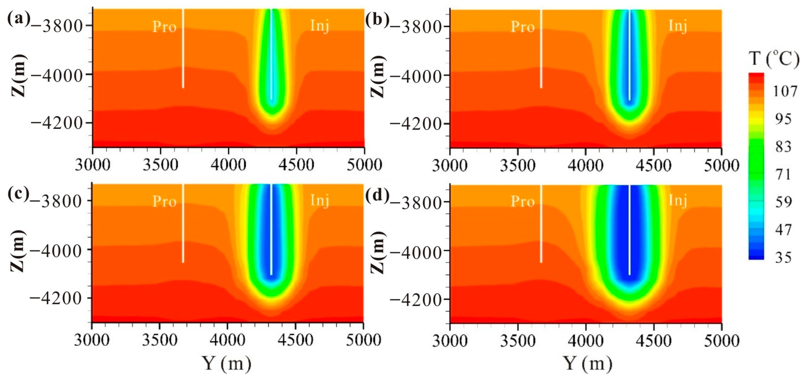
Figure 16. Reservoir temperature distribution variations with flow rate in the 50th year. (a) 40 m3/h; (b) 80 m3/h; (c) 120 m3/h; (d) 220 m3/h.
Water 17 03269 g016
Figure 17. Variations in wellhead temperature (a), HER (b), bottom production pressure (c), and bottom injection pressure (d) with time under different PLIs.
Water 17 03269 g017
Figure 18. Reservoir temperature distribution variations with PLIs in the 50th year. (a) 50 m; (b) 180 m; (c) 240 m; (d) 360 m.
Water 17 03269 g018
Figure 19. Variations in wellhead temperature (a), HER (b), bottom production pressure (c), and bottom injection pressure (d) with time under different injection temperatures.
Water 17 03269 g019
Figure 20. Reservoir temperature distribution of reservoir variations with injection temperature in the 50th year. (a) 30 °C; (b) 40 °C; (c) 50 °C; (d) 60 °C.
Water 17 03269 g020
Figure 21. Variations in wellhead temperature (a) and HER (b) with time.
Water 17 03269 g021
Figure 22. Flow rate variation (a) and temperature profile (b) along the open-hole section of the production well in the 50th year; variations in wellhead temperature (c) and HER (d) with time.
Water 17 03269 g022
Figure 23. Reservoir temperature distribution along the 2D cross section after 50 years for scenarios HC1–HC4. “Pro” represents the production well and “Inj” represents the injection well. (a) 2D temperature cross section of the scenario HC1; (b) 2D temperature cross section of the scenario HC2; (c) 2D temperature cross section of the scenario HC3; (d) 2D temperature cross section of the scenario HC4.
Water 17 03269 g023
Figure 24. (a) Variations in optimized wellhead temperatures of HC2, HC3 and HC4 with time; (b) Variations in optimized HERs of HC2, HC3 and HC4 with time.
Water 17 03269 g024
Table 1. Key hydrothermal parameters of the reservoirs in Panzhuang Uplift.
LayerPorosityPermeability
(m2)
Rock Gain Density
(kg/m3)
Specific Heat
(J/kg·°C)
Thermal Conductivity
(W/m·°C)
Q0.302.30 × 10−1326009191.8~2.3
Nm0.294.60 × 10−1326009581.68~2.5
Ng0.326.15 × 10−1326009091.68~2.5
Є0.058.23 × 10−1327608271.68~3.2
Qb0.052.09 × 10−1326008501.68~3.2
Jxw0.053.65 × 10−1326778382.93~4.00
Table 2. Composite sensitivities and identification of thermal parameters in the natural state model.
FormationRange
W/(m·°C)
Initial Value
W/(m·°C)
Optimal
Value
W/(m·°C)
95%
Confidence Interval
Sensitivity
Q1.80~2.302.052.301.51~3.090.22
Nm1.68~2.502.092.501.73~3.270.38
Ng1.68~2.502.092.501.35~3.650.12
Є1.68~3.202.442.791.60~3.970.14
Qb1.68~3.202.441.686.87 × 10−2~3.298.51 × 10−2
Jxw-42.93~4.003.474.002.46~5.540.11
Jxw-32.93~4.003.474.002.56~5.440.20
Jxw-22.93~4.003.472.932.31~3.550.16
Table 3. The observed variables in the pumping test of well CGSD-01.
Observed VariablesLarge
Drawdown
Middle
Drawdown
Small
Drawdown
Flow rate (m3/h)130.294.543.9
Wellhead temperature (°C)98.598.594.0
Groundwater depth (m)171.70143.48118.85
Time of duration (h)622416
Table 4. Composite sensitivities and identification of parameters in the history matching model.
ParameterRangeInitial ValueOptimal Value95%
Confidence Interval
Sensitivity
Bottom temperature (°C)110~122113.2120.26119.07~121.463.13 × 10−2
Permeability (m2)3.65 × 10⁻¹⁵~3.65 × 10−123.65 × 10−145.25 × 10−147.82 × 10⁻¹⁵~2.03 × 10−132.65 × 10¹¹
Table 5. Operation parameters of the designed geothermal doublet.
ParameterValue
Flow rate (m3/h)40~220, 80
Perforated length of injection well (m)50~360, 360
Perforated length of production well (m)336.68
Injection temperature (°C)30~60, 30
Wellbore radius (m)0.08
Table 6. The logging interpretation of the Wumishan Formation at well DL-48.
Sequence NumberStart Depth
(m)
End Depth
(m)
Thickness
(m)
Porosity
(%)
Permeability
(m2)
11869.51875.25.75.741.08 × 10−15
21884.21895.811.65.863.41 × 10−15
31909.81923.313.55.581.62 × 10−15
41927.91935.27.35.119.20 × 10−16
51942.71947.95.27.124.34 × 10−15
61955.21960.35.110.109.75 × 10−15
71973.31982.28.98.224.14 × 10−15
81987.61992.85.212.581.94 × 10−14
91997.62015.618.08.302.88 × 10−14
102023.32027.84.56.681.65 × 10−15
112036.32040.94.68.083.56 × 10−15
122043.82058.614.88.612.35 × 10−14
132080.62087.87.29.972.77 × 10−14
142154.12165.711.63.985.40 × 10−16
152170.92185.014.18.575.13 × 10−15
162214.72225.811.15.811.91 × 10−15
172255.72262.87.18.715.61 × 10−15
182273.92288.514.64.125.50 × 10−16
192316.52323.87.35.046.10 × 10−16
202339.62345.35.79.461.71 × 10−14
212367.72375.37.66.594.14 × 10−15
Disclaimer/Publisher’s Note: The statements, opinions and data contained in all publications are solely those of the individual author(s) and contributor(s) and not of MDPI and/or the editor(s). MDPI and/or the editor(s) disclaim responsibility for any injury to people or property resulting from any ideas, methods, instructions or products referred to in the content.